2.1 Environment

Time is discrete and continues forever. The economy consists of two countries, home and foreign, denoted as $h$ and $f$ , respectively. There are three currencies: a home currency, a foreign currency, and a global currency, which are denoted as currency $h, f, g$ , respectively. In each country $i \in \{h, f\}$ , the national money $M_{i}$ denominated in currency $i$ is supplied by the central bank of country $i$ . The supply of the global money $M_{g}$ is exogenously given. For simplicity, I assume that there is no interest payment on any currency. There is no aggregate uncertainty and thus the economy is deterministic.

There is a numeraire good, and the price of currency $\ell \in \{h, f, g\}$ in units of the numeraire good is denoted as $\phi _{\ell } \equiv 1/P_{\ell }$ , where $P_{\ell }$ is the price of the numeraire good in units of currency $\ell$ . Both countries face the same prices, so that the law of one price holds for the numeraire good. The nominal exchange rate of currency $f$ in units of currency $h$ is given by

(1) \begin{equation} \mathcal{E} = \frac {\phi _{f}}{\phi _{h}} = \frac {P_{h}}{P_{f}} \end{equation}

For example, an increase in $\mathcal{E}$ means depreciation of currency $h$ .

I focus on a stationary equilibrium where aggregate real balances are constant in each country. In such an economy, the money growth rate and the nominal interest rate on risk-free bonds are equivalent as a monetary policy instrument. Without loss of generality, the central bank sets the gross growth rate of money, $\gamma _{i} = M_{i}^{\prime }/M_{i}$ , in each country, where a variable with superscript $\prime$ indicates the variable in the next period. The growth rate of the global money is denoted as $\gamma _{g} = M_{g}^{\prime }/M_{g}$ .

Here, the nature of a global currency is in order. Although its details are not specified for simplicity, it can be a stablecoin such as Tether or USDC, which intends to be pegged to the US dollar. It can be a cryptoasset whose total supply is limited and predetermined. Or, although it has yet to emerge, it can be a CBDC that is issued by a third country and circulated across borders. In any case, for countries $h$ and $f$ , the global money is taken as exogenous. If the global currency takes the form of a stablecoin pegged to currency $f$ , or if the global currency takes the form of a CBDC issued by country $f$ , the growth rate of the global money is given by $\gamma _{g}=\gamma _{f}$ .

The situation of interest is such that both domestic and global currencies are valued and held in each country: $\phi _{\ell }\gt 0$ for all $\ell \in \{h, f, g\}$ . In this paper I exclusively focus on such a global-money economy. In addition, to shed light on the role of global money, I follow Benigno et al. (Reference Benigno, Schilling and Uhlig2022) and consider a situation in which the national money can be used for transactions only in the country of its origin, while the global money can be used in both countries.Footnote ⁴

In this environment, the question is whether the global-money economy restricts the conduct of monetary policy. Specifically, I am interested in whether a central bank continues to have autonomy in setting a monetary policy instrument in the global-money economy. To clarify the status of monetary policy, let me introduce the following two definitions.

Under monetary synchronization, the setting of a monetary policy instrument in one country is restricted to a certain value that depends on the setting of a monetary policy instrument in the other country. A special case is the equalization of the setting of a monetary policy instrument between the two countries, as studied by Benigno et al. (Reference Benigno, Schilling and Uhlig2022). Under monetary autonomy for one country, its central bank has a certain degree of freedom in setting its policy irrespective of the policy stance of the other country. In the economy without the global currency, monetary autonomy holds as in the standard two-country monetary model. The primary focus of this paper is whether monetary synchronization is an inevitable outcome in the global-money economy, or if monetary autonomy can be preserved.

2.2 Monetary synchronization

In this subsection, I argue that monetary synchronization arises in the global-money economy with no restriction on the portfolio choice of money. In country $h$ , a representative individual holds both currencies $h$ and $g$ and has real balances of $\phi _{h}m_{h}^{h} + \phi _{g}m_{h}^{\,g}$ , where $m_{h}^{j}$ denotes money denominated in currency $j$ (money $j$ for short hereafter) held by the individual in country $h$ . Since both currencies are valued and held, and since there is no restriction on holding both kinds of money, the individual is indifferent about holding money $h$ or $g$ . Although in general the liquidity service provided by money is an endogenous object, for the sake of exposition in this subsection only, let me assume that the liquidity service is identical between money $h$ and $g$ .Footnote ⁵ Then, the return of holding money $h$ , $\phi _{h}^{\prime }/\phi _{h}$ , has to be equated to that of holding money $g$ , $\phi _{g}^{\prime }/\phi _{g}$ . Since this arbitrage prevails in country $f$ as well, the returns of holding money $h$ and $f$ are equalized through the holding of the global money in both countries:

(2) \begin{equation} \frac {\phi _{h}^{\prime }}{\phi _{h}} = \frac {\phi _{g}^{\prime }}{\phi _{g}} = \frac {\phi _{f}^{\prime }}{\phi _{f}} \end{equation}

In a stationary equilibrium, aggregate real balances are constant so that the return of holding money $\ell \in \{h, f, g\}$ is equal to the inverse of the money growth rate $\gamma _{\ell }$ . Hence, equation (2) implies that the money growth rates are equalized between the two countries:

(3) \begin{equation} \gamma _{h} = \gamma _{g} = \gamma _{f} \end{equation}

Since equation (2) constitutes an equilibrium condition, in any stationary equilibrium in which the real balances of each currency is constant and positive over time, equation (2) has to hold and so does equation (3). Equation (3) shows a specific form of monetary synchronization, where the setting of the monetary policy instrument is equalized between the two countries.

Equation (2) is an application of Kareken and Wallace (Reference Kareken and Wallace1981) to an open economy with a global currency. Actually, equations (1) and (2) imply a constant nominal exchange rate:

(4) \begin{equation} \mathcal{E} = \frac {\phi _{f}}{\phi _{h}} = \frac {\phi _{f}^{\prime }}{\phi _{h}^{\prime }} = \mathcal{E}^{\prime } \end{equation}

Hence, in this economy, monetary synchronization arises in the form of equation (3) and at the same time the level of the nominal exchange rate is indeterminate as in Kareken and Wallace (Reference Kareken and Wallace1981).Footnote ⁶

2.3 Monetary autonomy

Monetary synchronization holds in the economy considered in Section 2.2, but the economy imposes specific assumptions on the environment as described in Section 2.1. Such assumptions comprise no restriction on holding money and an identical liquidity service between the national money and the global money.

In this subsection, I argue that monetary autonomy can be restored in the same environment with different assumptions. The core equation that gives rise to monetary synchronization is equation (2), which implies that the returns of holding different kinds of money are identical and thereby that the portfolio of real money balances is indeterminate. If equation (2) fails, monetary synchronization will break down and monetary autonomy will prevail.

Let $z_{i}^{\ell } \equiv \phi _{\ell }m_{i}^{\ell }$ denote the real balances of money $\ell \in \{h, f, g\}$ held by a representative individual in country $i \in \{h, f\}$ . Then, under the presumption that the individual in country $i$ holds money $i$ and $g$ only, the total real balances held by that individual is given by $z_{i} = z_{i}^{i} + z_{i}^{\,g}$ . Let me now drop the assumption of no restriction on holding money, and assume a specific form of friction that gives rise to the following constraint on the real balances of the global money: for $i \in \{h, f\}$

(5) \begin{equation} z_{i}^{\,g} \leq \bar {z}_{i}^{\,g}, \end{equation}

where $\bar {z}_{i}^{\,g}$ is an upper limit of the amount of the global money that can be used for a transaction by an individual in country $i$ . Here, the upper bound is exogenously given. It can be regarded as exogenous government policy that puts the upper limit on the use of the global money for a transaction. In Section 3.3, I will show how it can also be interpreted as an incentive constraint, a constraint that ensures no hidden action by buyers who pay using the global money. The intuition is that if a large volume of the global money is accepted by a seller, the buyer has an incentive to take a hidden action, such as counterfeiting, that will damage the seller. Constraint (5) prevents buyers from engaging in such an action.

Suppose that constraint (5) is binding. Then, the real balances of money $g$ are given by $z_{i}^{\,g} = \bar {z}_{i}^{\,g}$ for $i \in \{h,f\}$ . Then, the global money market clearing condition, $\phi _{g}M_{g} = z_{h}^{\,g} + z_{f}^{\,g}$ , determines the price of currency $g$ as

(6) \begin{equation} \phi _{g} = \frac {\bar {z}_{h}^{\,g} + \bar {z}_{f}^{\,g}}{M_{g}}. \end{equation}

In addition, since the total real balances $z_{i}$ are determined in each country in a typical monetary model as will be shown in Section 3, the real balances of the national money $i \in \{h,f\}$ are given by $z_{i}^{i} = z_{i} - \bar {z}_{i}^{\,g}$ . Then, the price of the national currency is determined by the national money market clearing condition as: for $i \in \{h, f\}$

(7) \begin{equation} \phi _{i} = \frac {z_{i} - \bar {z}_{i}^{\,g}}{M_{i}} \end{equation}

Combined with equation (1), equation (7) leads to the nominal exchange rate, given by

(8) \begin{equation} \mathcal{E} = \frac {M_{h}}{M_{f}}\frac {z_{f} - \bar {z}_{f}^{\,g}}{z_{h} - \bar {z}_{h}^{\,g}} \end{equation}

When the two countries are symmetric, equation (8) is reduced to $\mathcal{E}=M_{h}/M_{f}$ , so that the nominal exchange rate is simply given by the ratio of monetary aggregates between the two countries.

In a stationary equilibrium, the portfolios of real balances, the nominal exchange rate, and the prices of currencies are all determinate. And nothing forces the money growth rates to be equated between the two countries. From equations (6) and (7), the return of holding money $\ell \in \{h, f, g\}$ is given by $\phi _{\ell }^{\prime }/\phi _{\ell } = M_{\ell }/M_{\ell }^{\prime } = \gamma _{\ell }^{-1}$ . Since the binding constraint (5) prevents these returns from being equated, the central bank in each country has a certain degree of freedom in setting its money growth rate.

3.1 Common setup

Environment In addition to the model environment of Section 2.1, two countries, $h$ and $f$ , are populated with a continuum of $2n$ and $2$ agents, respectively, where $n \in (0, 1]$ denotes a relative population size of country $h$ . Agents in each country are evenly divided between buyers and sellers, so the size of sellers or buyers is $n$ and $1$ in country $h$ and $f$ , respectively. Each period consists of two sub-periods as in Lagos and Wright (Reference Lagos and Wright2005). In the first sub-period, agents meet bilaterally and at random in decentralized markets (DM) and trade the DM good. In the second sub-period, all agents meet in a friction-less centralized market (CM), trade the CM good, and exchange money. The CM good is taken as a numeraire. Both the DM and CM goods are perishable. In the DM, agents lack commitment and individual histories are private information, rendering unsecured credit unusable and making money essential as a medium of exchange.

Preferences and technologies In the DM, a seller in each country can produce the DM good, $q$ , with the cost $c(q)$ , but does not have utility over consumption. A buyer, on the other hand, has the utility, $u(q)$ , by consuming $q$ but cannot produce. In the CM, all agents get utility $U(y)$ by consuming the CM good, $y$ , which is produced according to a linear one-to-one technology in hours worked $x$ . Periodic utilities for a buyer and a seller, $\mathcal{U}^{B}$ and $\mathcal{U}^{S}$ , are assumed to be additively separable between the DM and CM goods and quasi-linear in hours worked:

(9) \begin{align} &\mathcal{U}^{B} = u(q) + U(y) - x\end{align}

(10) \begin{align}&\mathcal{U}^{S} = - c(q) + U(y) - x\end{align}

I assume that $u(\!\cdot\!)$ and $U(\!\cdot\!)$ are strictly increasing and strictly concave, $c(\!\cdot\!)$ is weakly convex, $u(0) = c(0)=U(0) = 0$ , and $c(\bar {q}) = u(\bar {q})$ for some $\bar {q}\gt 0$ . Agents discount the future between adjacent periods with a discount factor $\beta \in (0,1)$ .

Currencies As described in Section 2.1, three currencies are available: a home currency, a foreign currency, and a global currency. The corresponding monetary aggregate is denoted as $M_{\ell }$ and the associated growth rate is denoted as $\gamma _{\ell }=M_{\ell }^{\prime }/M_{\ell }$ for $\ell \in \{h, f, g\}$ . I assume that holding money is costly: $\gamma _{\ell } \gt \beta$ for all $\ell$ . Changes in the money supply are implemented through lump-sum monetary transfers in the CM to buyers. The way how lump-sum monetary transfers are distributed to buyers does not affect the results of this paper, but for simplicity, it is assumed that each buyer receives $\tau \equiv \sum _{\ell \in \{h,f,g\}}(\gamma _{\ell }-1)\phi _{\ell }M_{\ell }/(1+n)$ in both countries.

Matching In the DM, agents in both countries meet bilaterally and at random. Buyers are mobile while sellers are immobile. With probability $\alpha \in [0.5, 1]$ , a buyer from one country stays in the country, and with probability $1-\alpha$ , the buyer visits the other country. As in Zhang (Reference Zhang2014), the number of matches in the DM of country $i \in \{h,f\}$ is given by the matching function

\begin{equation*} \mathcal{M}_{i} \equiv \mathcal{M}\left (\mathcal{B}_{i}, \mathcal{S}_{i}\right ) = \frac {\mathcal{B}_{i}\mathcal{S}_{i}}{\mathcal{B}_{i} + \mathcal{S}_{i}} \end{equation*}

where $\mathcal{B}_{i}$ and $\mathcal{S}_{i}$ are the measures of buyers and sellers, respectively, in the DM of country $i$ . Then, the probability that a buyer from country $i$ meets a seller in country $j$ , denoted by $\mu _{ij}$ , is derived asFootnote ⁷

(11) \begin{align} \mu _{hh} = \frac {\alpha }{1+\alpha +(1-\alpha )/n},& &\mu _{hf} = \frac {1-\alpha }{1+\alpha + (1-\alpha )n} \notag \\ \mu _{fh} = \frac {1-\alpha }{1+\alpha +(1-\alpha )/n},& &\mu _{ff} = \frac {\alpha }{1+\alpha +(1-\alpha )n} \end{align}

If country $h$ is smaller than country $f$ and some buyers move to the different country, i.e., if $n\lt 1$ and $\alpha \lt 1$ , the probability of matching becomes asymmetric in the two countries. In the special case of $\alpha =1$ in which all buyers stay in their country, the probability of matching with a seller in the same country is reduced to $\mu _{hh}=\mu _{ff}=0.5$ , and the probability of matching with a seller in the different country is zero: $\mu _{hf}=\mu _{fh}=0$ .

Consumption and labor decisions in the CM Let $W_{i}^{\mathcal{B}}(\mathbf{z}_{i})$ and $V_{i}^{\mathcal{B}}(\mathbf{z}_{i})$ denote a value function of a buyer from country $i \ \in \{h,f\}$ with a portfolio of real balances $\mathbf{z}_{i}\equiv (z_{i}^{h}, z_{i}^{\,f}, z_{i}^{\,g})$ in the CM and the DM, respectively. In the CM, the problem of a typical buyer from country $i$ can be written as

(12) \begin{equation} W_{i}^{\mathcal{B}}(\mathbf{z}_{i}) = \max _{\{y, x, \mathbf{z}_{i}^{\prime }\}}\left\{U(y) - x + \beta V_{i}^{\mathcal{B}}(\mathbf{z}_{i}^{\prime })\right\} \end{equation}

subject to the flow budget constraint

(13) \begin{equation} y + \phi _{h}m_{i}^{h\prime } + \phi _{f}m_{i}^{\,f\prime } + \phi _{g}m_{i}^{\,g\prime } = x + z_{i}^{h} + z_{i}^{\,f} + z_{i}^{\,g} + \tau \end{equation}

The first-order condition with respect to $y$ yields

(14) \begin{equation} y = y^{\ast } \equiv U^{\prime -1}(1) \end{equation}

Since the real balances of money $\ell$ purchased today, $\phi _{\ell }m_{i}^{\ell \prime }$ , in the budget constraint (13) will be valued as $z_{i}^{\ell \prime } = \phi _{\ell }^{\prime }m_{i}^{\ell \prime }$ tomorrow, today’s real balances can be written as $\phi _{\ell }m_{i}^{\ell \prime } = (\phi _{\ell }/\phi _{\ell }^{\prime })z_{i}^{\ell \prime } = \gamma _{\ell }z_{i}^{\ell \prime }$ . By using this relationship and equation (14), substituting the budget constraint (13) into the problem (12) yields

(15) \begin{equation} W_{i}^{\mathcal{B}}(\mathbf{z}_{i}) = U(y^{\ast }) - y^{\ast } + z_{i}^{h} + z_{i}^{\,f} + z_{i}^{\,g} + \tau + \max _{\mathbf{z}_{i}^{\prime }}\left \{ - \gamma _{h}z_{i}^{h\prime } - \gamma _{f}z_{i}^{\,f\prime } - \gamma _{g}z_{i}^{\,g\prime } + \beta V_{i}^{\mathcal{B}}(\mathbf{z}_{i}^{\prime })\right \} \end{equation}

Equation (15) implies that the CM value function is linear in real balances, i.e., $W_{i}^{\mathcal{B}}(\mathbf{z}_{i}) = W_{i}^{\mathcal{B}}(\mathbf{0}) + z_{i}^{h}+z_{i}^{\,f}+z_{i}^{\,g}$ , and that the portfolio choice in the CM is independent of the current holdings of real balances.

Since holding money is costly, $\gamma _{\ell }\gt \beta$ for all $\ell \in \{h,f,g\}$ , sellers have no incentive to carry real balances either in the DM or the CM. Hence, the CM value function of a typical seller in country $j$ is given by

(16) \begin{equation} W_{j}^{\mathcal{S}}(\mathbf{z}_{j}) = U(y^{\ast }) - y^{\ast } + z_{j}^{h}+z_{j}^{\,f}+z_{j}^{\,g} + \beta V_{j}^{\mathcal{S}}(\mathbf{0}) \end{equation}

Terms of trade in the DM Upon matching with a seller in country $j$ , a buyer from country $i$ makes a take-it-or-leave-it offer to the seller.Footnote ⁸ The offer consists of a pair, $(\boldsymbol{d}_{ij}, q_{ij})$ , where $\boldsymbol{d}_{ij}\equiv (d_{ij}^{\,j}, d_{ij}^{\,g})$ is a portfolio of real balances of money $j$ and $g$ that the buyer pays to the seller, and $q_{ij}$ is the quantity of the DM good that the seller produces in exchange for receiving the payment. The total payment is $d_{ij} \equiv d_{ij}^{\,j} + d_{ij}^{\,g}$ . This offer takes into account the assumption that a seller in country $j$ does not receive the currency of the other country.

Consider a buyer from country $i$ who enters the DM with a portfolio of real balances, $\mathbf{z}_{i} \equiv (z_{i}^{h}, z_{i}^{\,f}, z_{i}^{\,g})$ . Since money is the only means of payment, the offer has to satisfy the payment constraint

(17) \begin{equation} d_{ij}^{\ell } \leq z_{i}^{\ell } \hspace {.5cm}\text{for $\ell \in \{j, g\}$} \end{equation}

Since holding money is costly, the constraint (17) holds with equality in equilibrium. Also, the seller’s value function (16) in the CM implies that the value function in the DM will also become linear in real balances, so that the seller accepts the offer if and only if the payment is no less than the cost of producing the DM good:

(18) \begin{equation} d_{ij}^{j}+d_{ij}^{\,g} - c(q_{ij}) \geq 0 \end{equation}

Constraint (18) holds with equality in equilibrium, otherwise, the buyer would be strictly better off by decreasing $d_{ij}^{j}$ or $d_{ij}^{\,g}$ , or increasing $q_{ij}$ .

3.2 The baseline model

Now I consider a case with no additional frictions, which is referred to as the baseline model. In this model, the only requirements for trade in the DM are constraints (17) and (18) that hold with equality. I show that monetary synchronization ensues in this global-money economy, articulating the idea presented in Section 2.2.

Value function in the DM Consider a buyer from country $i$ who enters the DM with a portfolio of real balances $\mathbf{z}_{i} \equiv (z_{i}^{h}, z_{i}^{\,f}, z_{i}^{\,g})$ . The buyer is matched with a seller in country $j$ with probability $\mu _{ij}$ . Upon the match, the buyer makes the take-it-or-leave-it offer of $(\boldsymbol{d}_{ij}, q_{ij})$ that satisfies constraints (17) and (18) with equality, and receives $q_{ij}$ in exchange for payment $d_{ij} = d_{ij}^{\,j} + d_{ij}^{\,g} = z_{i}^{\,j} + z_{i}^{\,g}$ . The buyer leaves the DM with utility $u(q_{ij})$ and the real balances of $z_{i}^{\,\hat {j}}$ unused for $\hat {j}\neq j$ . Since the value function of a buyer in the CM is linear in real balances as implied by equation (15), given the match, the buyer’s life-time utility in the DM can be written as $u(q_{ij}) + W_{i}^{\mathcal{B}}(\mathbf{0}) + z_{i}^{\,\hat {j}}$ . With probability $1- \mu _{ih}-\mu _{if}$ , the buyer is not matched with a seller. In this case, the buyer leaves the DM with periodic utility $u(0)=0$ and all real balances $\mathbf{z}_{i}$ unused. Then, the buyer’s life-time utility in the DM can be written as $W_{i}^{\mathcal{B}}(\mathbf{0}) + z_{i}^{h} + z_{i}^{\,f} + z_{i}^{\,g}$ . To summarize, the value function of the buyer in the DM is given by

(19) \begin{equation} V_{i}^{\mathcal{B}}(\mathbf{z}_{i}) = \mu _{ih}[ u(q_{ih}) + z_{i}^{\,f}] + \mu _{if}[ u(q_{if}) + z_{i}^{h}] + (1-\mu _{ih}-\mu _{if})(z_{i}^{h}+z_{i}^{\,f}+z_{i}^{\,g}) + W_{i}^{\mathcal{B}}(\mathbf{0}) \end{equation}

Since constraints (17) and (18) hold with equality, the quantity of the DM good in equation (19) is given by

(20) \begin{equation} q_{ij} = c^{-1}(z_{i}^{j} + z_{i}^{\,g}) \end{equation}

Equations (19) and (20) imply that the value function of a buyer in the DM depends only on the real balances brought from the CM in the previous period.

Portfolio choice in the CM With $V_{i}^{\mathcal{B}}(\mathbf{z}_{i})$ on hand, consider the buyer’s portfolio choice problem in the CM in equation (15). By pushing one period back and using equations (19) and (20), the problem can be written as

(21) \begin{align} \max _{\{z_{i}^{h}, z_{i}^{\,f}, z_{i}^{\,g}\}} & - \gamma _{h}z_{i}^{h} - \gamma _{f}z_{i}^{\,f} - \gamma _{g}z_{i}^{\,g} + \beta \biggl \{\mu _{ih}\left [u \left ( c^{-1}(z_{i}^{h}+z_{i}^{\,g})\right ) + z_{i}^{\,f}\right ] \notag \\ &+\mu _{if}\left [u\left (c^{-1}(z_{i}^{\,f}+z_{i}^{\,g})\right ) + z_{i}^{h}\right ] + (1-\mu _{ih}-\mu _{if})(z_{i}^{h}+z_{i}^{\,f}+z_{i}^{\,g})\biggl \} \end{align}

Given that the matching probabilities, $\mu _{ih}$ and $\mu _{if}$ , are strictly positive, an interior solution has to satisfy the first-order conditions with respect to $z_{i}^{h}$ , $z_{i}^{\,f}$ , and $z_{i}^{\,g}$ , which are given, respectively, by

(22) \begin{align}& \frac {\gamma _{h}}{\beta }-1 = \mu _{ih} \left [\frac {u^{\prime }\left ( c^{-1}(z_{i}^{h}+z_{i}^{\,g})\right )}{c^{\prime }\left (c^{-1}(z_{i}^{h}+z_{i}^{\,g})\right )}-1\right ]\end{align}

(23) \begin{align}& \frac {\gamma _{f}}{\beta }-1 = \mu _{if} \left [\frac {u^{\prime }\left ( c^{-1}(z_{i}^{\,f}+z_{i}^{\,g})\right )}{c^{\prime }\left (c^{-1}(z_{i}^{\,f}+z_{i}^{\,g})\right )}-1\right ]\end{align}

(24) \begin{align}\frac {\gamma _{g}}{\beta }-1 = \mu _{ih} \left [\frac {u^{\prime }\left ( c^{-1}(z_{i}^{h}+z_{i}^{\,g})\right )}{c^{\prime }\left (c^{-1}(z_{i}^{h}+z_{i}^{\,g})\right )}-1\right ] + \mu _{if}\left [\frac {u^{\prime }\left ( c^{-1}(z_{i}^{\,f}+z_{i}^{\,g})\right )}{c^{\prime }\left (c^{-1}(z_{i}^{\,f}+z_{i}^{\,g})\right )}-1\right ]\end{align}

where $u^{\prime }(\!\cdot\!)$ and $c^{\prime }(\!\cdot\!)$ denote the derivatives of functions $u(\!\cdot\!)$ and $c(\!\cdot\!)$ , respectively. In each equation, the left-hand side is the opportunity cost of holding money and the right-hand side captures the liquidity service of money – the expected marginal benefit of holding real balances, $u^{\prime }(\!\cdot\!)/c^{\prime }(\!\cdot\!)$ , in excess of the benchmark of $1 = u^{\prime }(q^{\ast })/c^{\prime }(q^{\ast })$ . The complete characterization of the solution of the problem (21), which takes into account corner solutions, can be found in Appendix A.2.

Monetary synchronization Combining equations (22)-(24) yields

(25) \begin{equation} \gamma _{h} + \gamma _{f} = \gamma _{g} + \beta \end{equation}

This condition requires that the sum of the growth rates of money in the two countries be constant for given $\gamma _{g}$ . The setting of the monetary policy instrument in one country is tied to the setting of the monetary policy instrument in the other country, and hence this global-money economy features monetary synchronization.

To obtain the intuition of condition (25), let $i_{\ell } \equiv \gamma _{\ell }/\beta -1$ denote the opportunity cost of holding money $\ell$ . Then, condition (25) can be written as

(26) \begin{equation} i_{g} = i_{h} + i_{f} \end{equation}

This equation implies that the cost of holding the global money is equated to the sum of the costs of holding money $h$ and money $f$ . Since the global money can be used in both countries while the national money $j \in \{h,f\}$ can be used only in country $j$ , holding the global money brings the sum of the benefits of holding the two kinds of money, which corresponds to the right-hand side of equation (24). The benefit of holding money $\ell \in \{h,f,g\}$ is equated to its opportunity cost in equilibrium, leading to equation (26).

Special case To map this model and the main idea described in Section 2.2, consider a special case of $\alpha =1$ in which all buyers stay in their country: $\mu _{hf}=\mu _{fh}=0$ . In this case, buyers from country $i$ hold money $i$ and $g$ only, as assumed in Section 2.2. Then, given an interior solution, the first-order conditions of the problem (21) are reduced to

(27) \begin{align}\frac {\gamma _{i}}{\beta }-1 = \mu _{ii} \left [\frac {u^{\prime }\left ( c^{-1}(z_{i}^{i}+z_{i}^{\,g})\right )}{c^{\prime }\left (c^{-1}(z_{i}^{i}+z_{i}^{\,g})\right )}-1\right ] \hspace {.5cm}\text{for $i\in \{h,f\}$}\end{align}

(28) \begin{align}\frac {\gamma _{g}}{\beta }-1 = \mu _{ii} \left [\frac {u^{\prime }\left ( c^{-1}(z_{i}^{i}+z_{i}^{\,g})\right )}{c^{\prime }\left (c^{-1}(z_{i}^{i}+z_{i}^{\,g})\right )}-1\right ]\end{align}

These equations imply the equalization of the money growth rates, $\gamma _{h}=\gamma _{g}=\gamma _{f}$ , as in equation (3). In addition, the liquidity service of money, which is captured by the right-hand side of equations (27) and (28), is identical between money $h$ , $f$ , and $g$ , as assumed in Section 2.2. Hence, this special case provides solid micro-foundations for the idea of monetary synchronization presented in Section 2.2.

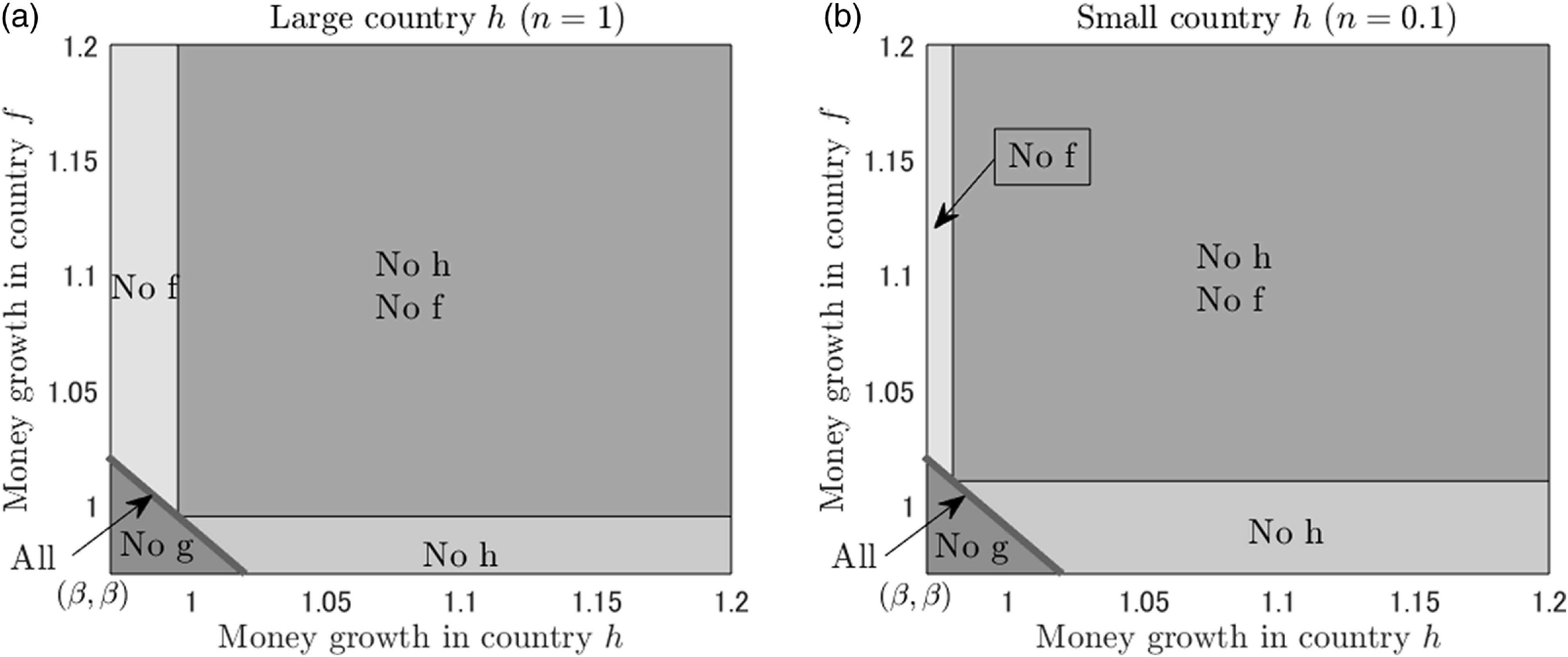
International monetary system Thus far, attention has been restricted to the global-money economy in which all currencies are circulated. What if one country deviates from condition (25)? Does a different international monetary system emerge where a different set of currencies is circulated?

Figure 1 shows which international monetary system emerges as a function of monetary policy settings in countries $h$ and $f$ for given $\gamma _{g}$ for two cases: country $h$ as a large economy ( $n=1$ ) and a small economy ( $n=0.1$ ).Footnote ⁹ In the case of $n=1$ , the two countries are symmetric. The region of the global-money economy that features monetary synchronization is depicted as the dark gray line, dubbed as ‘All.’ Above the line, there are three regions: no circulation of currency $h$ (‘No $h$ ’); no circulation of currency $f$ (‘No $f$ ’); no circulation of currencies $h$ and $f$ (‘No $h$ No $f$ ’). Intuitively, if $\gamma _{h}$ is raised above the line of monetary synchronization when $\gamma _{f}$ is relatively low, the opportunity cost of holding currency $h$ becomes so high that no one is willing to hold currency $h$ . The same can be said for currency $f$ , and if both $\gamma _{h}$ and $\gamma _{f}$ become higher than a certain level, both currencies cease to circulate while only the global currency circulates in the economy. Conversely, if $\gamma _{h}$ or $\gamma _{f}$ is lowered below the line of monetary synchronization, sovereign currencies become so attractive that no one is willing to hold the global currency.

Figure 1.

Monetary policy and international monetary system in the baseline model.

Note: ‘All’ indicates the circulation of all currencies. ‘No $\ell$ ’ indicates no circulation of currency $\ell \in \{h,f,g\}$ .

Similar results continue to hold in the case of country $h$ as a small country, as shown in Figure 1(b). Compared to the case of country $h$ as a large country, the region of ‘No $h$ ’ is expanded while the region of ‘No $f$ ’ is shrunk. Intuitively, as the relative size of country $h$ becomes smaller, buyers become less likely to meet sellers in country $h$ as in equation (11), which makes currency $h$ less useful, resulting in asymmetric regions of ‘No $h$ ’ and ‘No $f$ ’ in the figure. The analytical results that characterize all types of international monetary system can be found in Appendix A.2.

Nominal exchange rate indeterminacy Under monetary synchronization, nominal exchange rates become indeterminate. The equilibrium conditions of the buyer’s portfolio choice (22)–(24) can be replaced with equations (22), (23), and (25). Since equation (25) pertains to the restriction on money growth rates – monetary synchronization, there are only two equations (22) and (23) for three unknowns: $z_{i}^{h}$ , $z_{i}^{\,f}$ , and $z_{i}^{\,g}$ . And thus the buyer’s portfolio is indeterminate: buyers are indifferent as to the composition of the quantities of real balances of currency $\ell \in \{h,f\}$ and currency $g$ . This leads to the indeterminacy of prices of currencies. The money market clearing conditions are $\phi _{\ell }M_{\ell }=z_{h}^{\ell } + z_{f}^{\ell }$ for currency $\ell \in \{h,f,g\}$ . Since the right-hand side is indeterminate, so is the price of currency $\phi _{\ell }$ in the left-hand side of the equation. As the nominal exchange rate is given by the relative price of home and foreign currencies (1), the nominal exchange rate is also indeterminate. This result motivates the paper to introduce frictions that resolve the nominal exchange rate indeterminacy as a way to restore monetary autonomy.

3.3 Currency counterfeiting

In this subsection, I add a specific friction in the form of currency counterfeiting and imperfect recognizability to the common setup of Section 3.1 and show that, unlike the economy considered in Section 3.2, monetary autonomy can be preserved in the global-money economy. As mentioned in the Introduction, what is important for restoring monetary autonomy is a liquidity constraint for the use of global money, which is derived endogenously under currency counterfeiting and imperfect recognizability. An exogenous liquidity constraint in the form of government policy that limits the use of global money can also restore monetary autonomy.

Recognizability problem The national currencies are perfectly recognizable by sellers, so there is no counterfeiting of the national currencies as in the previous subsection. But here I assume that the global currency can be counterfeited by buyers and is imperfectly recognizable by sellers.Footnote ¹⁰ Specifically, sellers are unable to distinguish genuine global money from counterfeit global money in the DM, and buyers can produce counterfeit digital currencies of the global currency at the end of each period – between the closure of the CM and the opening of the DM. For simplicity, following Nosal and Rocheteau (Reference Nosal and Rocheteau2017, Chapter 12), I assume that producing counterfeit digital currencies entails a fixed cost of $\psi \gt 0$ only and the variable cost is zero. Then, by spending $\psi \gt 0$ , a buyer can produce any amount of counterfeit global digital currencies. In addition, counterfeits produced in the previous period are all detected and confiscated when agents enter the CM today. Hence, in each period a buyer incurs the fixed cost to enter the DM with counterfeits in hand.

Incentive constraint In general, a buyer chooses a portfolio of genuine global money and counterfeit global money, but this choice can be simplified as follows. Since increasing the holding of genuine money is costly, but increasing the holding of counterfeit money is free if the fixed cost is already paid, a buyer holds either genuine global money or counterfeit global money, but not both. In addition, holding more counterfeits than those used in the DM generates no benefit since all the unused counterfeits will be confiscated in the following CM. Hence, a buyer from country $i$ accumulates either the real balances $z_{i}^{\,g}$ of the genuine global money or the real balances $z_{i}^{\,g}$ of the counterfeit global money. The associated costs of doing so are $\gamma _{g}z_{i}^{\,g}$ and $\psi$ , respectively.Footnote ¹¹ Then, the buyer has no incentive to counterfeit if $\gamma _{g} z_{i}^{\,g} \leq \psi$ , or

(29) \begin{equation} z_{i}^{\,g} \leq \frac {\psi }{\gamma _g} \end{equation}

Since the payment constraint (17) holds with equality, a take-it-or-leave-it offer made by the buyer satisfies $d_{ij}\equiv (d_{ij}^{j},d_{ij}^{\,g}) = (z_{i}^{j}, z_{i}^{\,g})$ . Then, the incentive constraint (29) can be written as

(30) \begin{equation} d_{ij}^{\,g} \leq \frac {\psi }{\gamma _{g}} \end{equation}

Upon receiving the offer, if the offer satisfies the incentive constraint (30), the seller finds that the global money used for the payment is genuine. If the constraint (30) does not hold, then I assume that the seller believes that the global money used for the payment is counterfeited. In this case, the seller rejects the offer even if it satisfies the participation constraint (18) with equality, since the constraint fails to hold ex-post once the seller has found that the global money is counterfeited. Hence, the incentive constraint (30) constitutes a necessary condition for the seller to accept the offer.

No double spending While counterfeiting with the fixed cost of $\psi$ is a parsimonious way to derive the liquidity constraint (30) endogenously, it can be derived as a no-double-spending constraint for a cryptocurrency that employs a consensus protocol based on proof-of-work. Here, double spending by a buyer is equivalent to faking payment $d_{ij}^{\,g}=z_{i}^{\,g}$ to a seller without using the actual real balances of digital money $z_{i}^{\,g}$ , while receiving the good produced by the seller. As shown by Chiu and Koeppl (Reference Chiu and Koeppl2022), for a cryptocurrency with a proof-of-work protocol, a buyer has no incentive to double spend if and only if the amount of the payment in the cryptocurrency is limited as

(31) \begin{equation} d_{ij}^{\,g} \leq R (N+1)N \end{equation}

where $R$ is a reward for mining – updating a record of transactions (blockchain) – and $N$ is a confirmation lag – the number of confirmations in updating blockchains, where the good is produced and transferred to the buyer after the $N$ th confirmation.

The no-double-spending constraint (31) is intuitive. The left-hand-side of (31) is the benefit obtained when succeeding in double spending, and the right-hand-side of (31) captures the cost of double spending. It is increasing in the reward $R$ , since the incentives of miners to compete for updating blockchains increase as $R$ increases. It is increasing exponentially in $N$ , since winning the competition of mining for $N$ consecutive times, which is required for double spending, becomes much more difficult as $N$ increases.

The reward $R$ and the confirmation lag $N$ can be endogenized as in Chiu and Koeppl (Reference Chiu and Koeppl2022), but doing so would not affect the main results of this paper as long as the constraint (31) is binding. For example, $R$ can be financed by seigniorage by assuming $\gamma _{g}\gt 1$ . In this case the lump-sum monetary transfers do not include the seigniorage and are given by $\tau \equiv \sum _{\ell \in \{h,f\}}(\gamma _{\ell }-1)\phi _{\ell }M_{\ell }/(1+n)$ . An important point here is that the parsimonious incentive constraint (30) can be obtained by considering a cryptocurrency with a proof-of-work protocol as a global digital currency in this model.

Portfolio choice in the CM Given that the offer is accepted by the seller, the DM value function of the buyer is given by equation (19) as in the baseline model in Section 3.2. With the DM value function on hand, the buyer’s portfolio choice problem in the CM is given by (21) – the same maximization problem as in the baseline model – but subject to the incentive constraint (29).Footnote ¹² Let $\xi _{i}$ denote a Lagrange multiplier on the constraint. Given that the holding of real balances is positive for all kinds of money, the first-order conditions with respect to $z_{i}^{h}$ , $z_{i}^{\,f}$ , and $z_{i}^{\,g}$ are given, respectively, by equations (22) and (23), and

(32) \begin{equation} \frac {\gamma _{g}+\xi _{i}}{\beta }-1 = \mu _{ih} \left [\frac {u^{\prime }\left ( c^{-1}(z_{i}^{h}+z_{i}^{\,g})\right )}{c^{\prime }\left (c^{-1}(z_{i}^{h}+z_{i}^{\,g})\right )}-1\right ] + \mu _{if}\left [\frac {u^{\prime }\left ( c^{-1}(z_{i}^{\,f}+z_{i}^{\,g})\right )}{c^{\prime }\left (c^{-1}(z_{i}^{\,f}+z_{i}^{\,g})\right )}-1\right ] \end{equation}

The only difference between condition (32) in this economy and condition (24) in the baseline model is the presence of the multiplier $\xi _{i}$ in equation (32). The complete characterization of the solution of the portfolio choice problem, which takes into account corner solutions, can be found in Appendix A.4.

Monetary autonomy Combining equations (22), (23), and (32) yields

(33) \begin{equation} \xi _{i} = \gamma _{h} + \gamma _{f} - \gamma _{g} - \beta \end{equation}

This condition suggests that as long as $\xi _{i}\gt 0$ , monetary autonomy can be restored in the global-money economy. Formally, the existence of monetary autonomy is established in the following proposition.

Proposition 1. Define $\Psi (z) := u^{\prime }(c^{-1}(z))/c^{\prime }(c^{-1}(z))-1$ . Assume that for given $\gamma _{g}$ the cost of counterfeiting is not large enough to satisfy

(34) \begin{equation} \psi \lt \gamma _{g}\Psi ^{-1}\left (\frac {\gamma _{g}-\beta }{\beta \mu _{ii}}\right ). \end{equation}

for country $i \in \{h,f\}$ . Then, any pair of monetary policies, $\{\gamma _{h},\gamma _{f}\}$ , that are chosen from the following set that is neither empty nor a singleton,

(35) \begin{equation} \gamma _{i}\in \big (\gamma _{g}-(\gamma _{j}-\beta ),\,\, \beta + \beta \mu _{ii}\Psi (\bar {z}^{\,g})\big ), \end{equation}

for $i,j\in \{h,f\}$ with $j\neq i$ , constitutes an equilibrium in which the global currency is circulated in both countries and at least the domestic currency is circulated in each country.

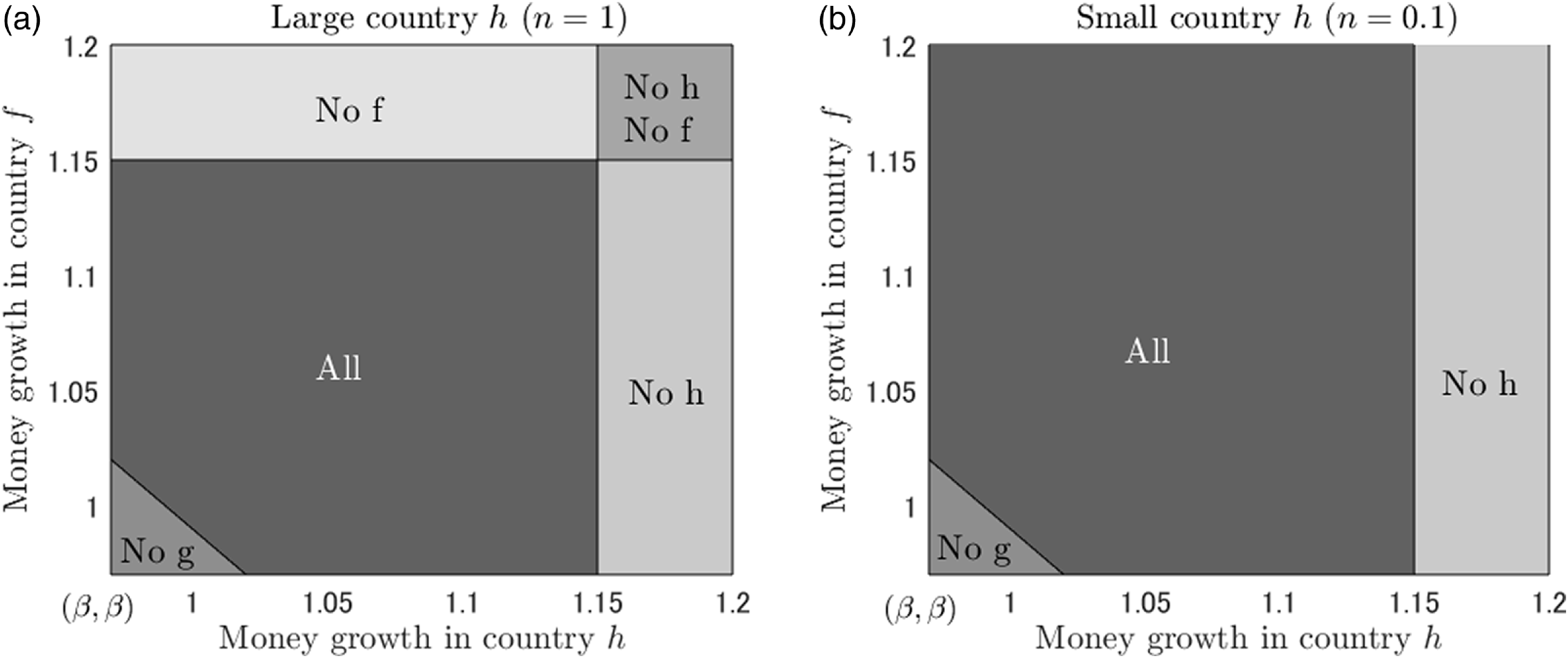
Figure 2 illustrates the emergence of monetary autonomy in the model with currency counterfeiting.Footnote ¹³ The region where all currencies are circulated, dubbed as ‘All,’ is now enlarged, which makes a contrast to the baseline model where such a region is just a line, shown in Figure 1. For any monetary policy in country $f$ , the central bank in country $h$ can set its policy $\gamma _{h}$ from the set that is neither empty nor a singleton, given by (35), without losing the status of its currency circulating in the domestic economy. Since the incentive constraint (29) is binding, there is certain demand for the domestic money as long as its growth rate is not too high, giving rise to monetary autonomy. If the size of country $h$ becomes relatively small at $n=0.1$ , the size of country $f$ becomes relatively large, and the region of no circulation of currency $f$ , dubbed as ‘No f,’ is shrunk and then disappears in Figure 2(b). This is intuitive because a large country size means that a buyer is more likely to be matched with a seller in the country, making the currency more useful as a medium of exchange.

Figure 2.

Monetary policy and international monetary system in the model with currency counterfeiting.

Note: ‘All’ indicates the circulation of all currencies. ‘No $\ell$ ’ indicates no circulation of currency $\ell \in \{h,f,g\}$ .

Condition (34) in Proposition 1 ensures that the set of money growth rates, given by (35), that can be chosen by country $i\in \{h,f\}$ without losing the status of the circulation of the currency is neither empty nor a singleton. Condition (34) requires that when $\gamma _{i}$ is set to $\gamma _{i}=\gamma _{g}$ , the portfolio share of the global currency, $z_{i}^{\,g}/(z_{i}^{i} + z_{i}^{\,g})$ , is less than unity, which is about $0.7$ in the numerical illustration of Figure 2(a). Condition (34) also implies that the cost of counterfeiting is less than the value of portfolios of domestic and global money that are chosen when $\gamma _{g}=1$ .

Special case As in Section 3.2, consider a special case of $\alpha =1$ in which all buyers stay in their country. Then, given that the holding of each money is positive, the first-order conditions of the buyer’s portfolio choice problem in the DM are reduced to equation (27) and

(36) \begin{equation} \frac {\gamma _{g}+\xi _{i}}{\beta }-1 = \mu _{ii} \left [\frac {u^{\prime }\left ( c^{-1}(z_{i}^{i}+z_{i}^{\,g})\right )}{c^{\prime }\left (c^{-1}(z_{i}^{i}+z_{i}^{\,g})\right )}-1\right ] \end{equation}

Combining equations (27) and (36) yields

(37) \begin{equation} \xi _{i} = \gamma _{i} - \gamma _{g} \end{equation}

In this case, when the cost of counterfeiting is small enough to satisfy condition (34), the region of monetary autonomy is given by $\big (\gamma _{g}, \beta +\beta \mu _{ii}\Psi (\bar {z}^{\,g})\big )$ . In this economy, the upper bound $\bar {z}_{i}^{\,g}$ in the ad hoc constraint (5) in the simple framework discussed in Section 2.3 corresponds to $\psi /\gamma _{g}$ in the incentive constraint (29), and the total real balances, $z_{i}=z_{i}^{i}+z_{i}^{\,g}$ , are determined by equation (27). Hence, the price of the global currency, the price of each national currency, and the nominal exchange rate are determined by equations (6)–(8), respectively, as in Section 2.3.

3.4 Government transaction policy

I now consider a different friction in the DM: government transaction policy. I add such a friction to the common setup of Section 3.1 and show that monetary autonomy can be preserved in the global-money economy.

Government sellers Thus far, I have assumed that sellers are private sellers who behave in their own interests. In this subsection, I introduce government sellers who follow an exogenous policy on which currency they should accept. Specifically, reflecting the fact that, in practice, the tax liabilities of households and firms have to be paid in domestic money in almost all countries, I assume that government sellers in country $j$ accept the national currency of country $j$ only. In each country $j \in \{h, f\}$ , a fraction of government sellers is assumed to be $0 \leq \tilde {\mu }_{j} \leq 1$ . Then, for a buyer from country $i$ , the probability of matching with a private seller in country $j$ , who can accept both the national currency and the global currency, is $\mu _{ij}(1-\tilde {\mu }_{j})$ , and the probability of matching with a government seller in country $j$ , who can accept the national currency only, is $\mu _{ij}\tilde {\mu }_{j}$ .

The terms of trade with a government seller in the DM differ from those with a private seller since a government seller can accept the national currency only. A take-it-or-leave-it offer made by a buyer from country $i$ to a government seller in country $j$ consists of a pair $(\tilde {d}_{ij}^{j}, \tilde {q}_{ij})$ , where $\tilde {d}_{ij}^{j}$ is the payment using the national currency $j$ in country $j$ and $\tilde {q}_{ij}$ is the quantity of the DM good produced by the government seller. This offer has to satisfy the payment constraint similar to (17),

(38) \begin{equation} \tilde {d}_{ij}^{j} \leq z_{i}^{j} \end{equation}

and the modified participation constraint,

(39) \begin{equation} \tilde {d}_{ij}^{j}-c(\tilde {q}_{ij})\geq 0. \end{equation}

These constraints reflect the fact that the government seller can accept the national currency $j$ only. The terms of trade with a private seller remain the same as in the common setup of Section 3.1.

Value function in the DM Consider a match in the DM for a buyer from country $i$ with a portfolio of real balances 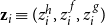$\mathbf{z}_{i}\equiv (z_{i}^{h}, z_{i}^{\,f}, z_{i}^{\,g})$ . For the purpose of exposition, I focus on a case where the payment constraint (17) is binding for all matches.Footnote ¹⁴ In this case, with probability $\mu _{ij}(1-\tilde {\mu }_{j})$ , the buyer is matched with a private seller in country $j$ and makes an offer $(d_{ij}, q_{ij})$ that satisfies conditions (17) and (18). The resulting life-time utility of the buyer is $u(q_{ij}) + W_{i}^{\mathcal{B}}(\boldsymbol{0}) + z_{i}^{\,\hat {j}}$ for $\hat {j} \neq j$ as in the baseline model in Section 3.2. With probability $\mu _{ij}\tilde {\mu }_{j}$ , the buyer is matched with a government seller in country $j$ and makes an offer $(\tilde {d}_{ij}^{j}, \tilde {q}_{ij})$ that satisfies conditions (38) and (39). The buyer leaves the DM with monies $\hat {j}$ and $g$ unused, so that the buyer’s life-time utility is given by $u(\tilde {q}_{ij}) + W_{i}^{\mathcal{B}}(\boldsymbol{0}) + z_{i}^{\,\hat {j}} + z_{i}^{\,g}$ . With probability $1-\mu _{ih}-\mu _{if}$ , the buyer is unmatched with a seller. Then, the DM value function of the buyer can be written as

\begin{align*} V_{i}^{\mathcal{B}}(\mathbf{z}_{i}) &= \mu _{ih}(1-\tilde {\mu }_{h})[ u(q_{ih}) + z_{i}^{\,f}] + \mu _{ih}\tilde {\mu }_{h}[ u(\tilde {q}_{ih}) + z_{i}^{\,f} + z_{i}^{\,g}] \\ &+ \mu _{if}(1-\tilde {\mu }_{f})[ u(q_{if}) + z_{i}^{h}] + \mu _{if}\tilde {\mu }_{f}[ u(\tilde {q}_{if}) + z_{i}^{h} + z_{i}^{\,g}] \\ &+ (1-\mu _{ih}-\mu _{if})(z_{i}^{h}+z_{i}^{\,f} + z_{i}^{\,g}) + W_{i}^{\mathcal{B}}(\boldsymbol{0}) \end{align*}

Since the constraints (17), (18), and (39) hold with equality, the quantity of the DM good produced by a private seller and a government seller is given by equation (20) and $\tilde {q}_{ij} = c^{-1}(z_{i}^{j})$ , respectively.

Portfolio choice in the CM Similarly to the formulation in Section 3.2, the buyer’s portfolio choice problem in the CM can be written as

\begin{align*} \max _{\{z_{i}^{h}, z_{i}^{\,f}, z_{i}^{\,g}\}} & - \gamma _{h}z_{i}^{h} - \gamma _{f}z_{i}^{\,f} - \gamma _{g}z_{i}^{\,g} + \beta \biggl \{\mu _{ih}(1-\tilde {\mu }_{h})\left [u \left ( c^{-1}(z_{i}^{h}+z_{i}^{\,g})\right ) + z_{i}^{\,f}\right ] \\ & + \mu _{ih}\tilde {\mu }_{h}\left [u\left (c^{-1}(z_{i}^{h})\right ) + z_{i}^{\,f} + z_{i}^{\,g}\right ] +\mu _{if}(1-\tilde {\mu }_{f})\left [u\left (c^{-1}(z_{i}^{\,f}+z_{i}^{\,g})\right ) + z_{i}^{h}\right ] \\ & +\mu _{if}\tilde {\mu }_{f}\left [ u\left ( c^{-1}(z_{i}^{\,f})\right ) + z_{i}^{h} + z_{i}^{\,g}\right ] + (1-\mu _{ih}-\mu _{if})(z_{i}^{h}+z_{i}^{\,f}+z_{i}^{\,g})\biggl \} \end{align*}

The first-order conditions with respect to $z_{i}^{h}$ , $z_{i}^{\,f}$ , and $z_{i}^{\,g}$ for their interior solution are given, respectively, as

(40) \begin{align}\frac {\gamma _{h}}{\beta }-1 = \mu _{ih}(1-\tilde {\mu }_{h}) \left [\! \frac {u^{\prime }\left ( c^{-1}(z_{i}^{h}+z_{i}^{\,g})\right )}{c^{\prime }\left (c^{-1}(z_{i}^{h}+z_{i}^{\,g})\right )}-1\right ]\! + \mu _{ih}\tilde {\mu }_{h}\left [\! \frac {u^{\prime }\left ( c^{-1}(z_{i}^{h})\right )}{c^{\prime }\left (c^{-1}(z_{i}^{h})\right )}-1\right ]\end{align}

(41) \begin{align}\frac {\gamma _{f}}{\beta }-1 = \mu _{if}(1-\tilde {\mu }_{f}) \left [\! \frac {u^{\prime }\left ( c^{-1}(z_{i}^{\,f}+z_{i}^{\,g})\right )}{c^{\prime }\left (c^{-1}(z_{i}^{\,f}+z_{i}^{\,g})\right )}-1\right ]\! + \mu _{if}\tilde {\mu }_{f}\left [\! \frac {u^{\prime }\left ( c^{-1}(z_{i}^{\,f})\right )}{c^{\prime }\left (c^{-1}(z_{i}^{\,f})\right )}-1\right ]\end{align}

(42) \begin{align}\frac {\gamma _{g}}{\beta }-1 = \mu _{ih}(1-\tilde {\mu }_{h}) \left [\! \frac {u^{\prime }\left ( c^{-1}(z_{i}^{h}+z_{i}^{\,g})\right )}{c^{\prime }\left (c^{-1}(z_{i}^{h}+z_{i}^{\,g})\right )}-1\right ]\! + \mu _{if}(1-\tilde {\mu }_{f})\left [\! \frac {u^{\prime }\left ( c^{-1}(z_{i}^{\,f}+z_{i}^{\,g})\right )}{c^{\prime }\left (c^{-1}(z_{i}^{\,f}+z_{i}^{\,g})\right )}-1\right ]\end{align}

Compared to equations (22)-(24) in the baseline model, holding the national money has additional benefits as appeared in the second term in the right-hand-side of equations (40) and (41) due to the presence of government sellers who accept the national money only. If there are no government sellers, i.e., $\tilde {\mu }_{h}=\tilde {\mu }_{f}=0$ , equations (40)–(42) are reduced to equations (22)-(24) in the baseline model.

Monetary autonomy For given $\gamma _{h}$ , $\gamma _{f}$ , and $\gamma _{g}$ , the three equations (40)–(42) provide a solution for $z_{i}^{h}$ , $z_{i}^{\,f}$ , and $z_{i}^{\,g}$ . For given $\gamma _{g}$ , a pair of $(\gamma _{h}, \gamma _{f})$ that ensures an interior solution constitutes an area of monetary autonomy in the global-money economy. The presence of government sellers ensures the circulation of the domestic currency unless there is hyperinflation (see Appendix A.6). An attention is restricted to the case of no hyperinflation. In addition, for simplicity, a fraction of government sellers is assumed to be identical between the two countries: $\tilde {\mu }=\tilde {\mu }_{h}=\tilde {\mu }_{f}$ . By combining equations (40)–(42), a condition for the existence of an equilibrium with positive holdings of the global money is derived asFootnote ¹⁵

(43) \begin{equation} \gamma _{h} + \gamma _{f} - \gamma _{g} - \beta \gt \frac {\tilde {\mu }(\gamma _{g}-\beta )}{1-\tilde {\mu }} \end{equation}

If there are no government sellers, $\tilde {\mu }=0$ , the left-hand-side of this inequality should be positive, but it does not hold since conditions (40)–(42) are reduced to condition (25) if $\tilde {\mu }=0$ . Condition (43) suggests that given $\gamma _{f}$ and $\gamma _{g}$ , the money growth rate of the home country within the range of $\gamma _{h}\gt \underline {\gamma }_{h}$ can support a global money equilibrium in which all currencies are valued and circulated, where the lower bound is implied by condition (43) as $\underline {\gamma }_{h}\equiv \gamma _{g}-\gamma _{f}+\beta - \tilde {\mu }(\gamma _{g}-\beta )/(1-\tilde {\mu })$ . 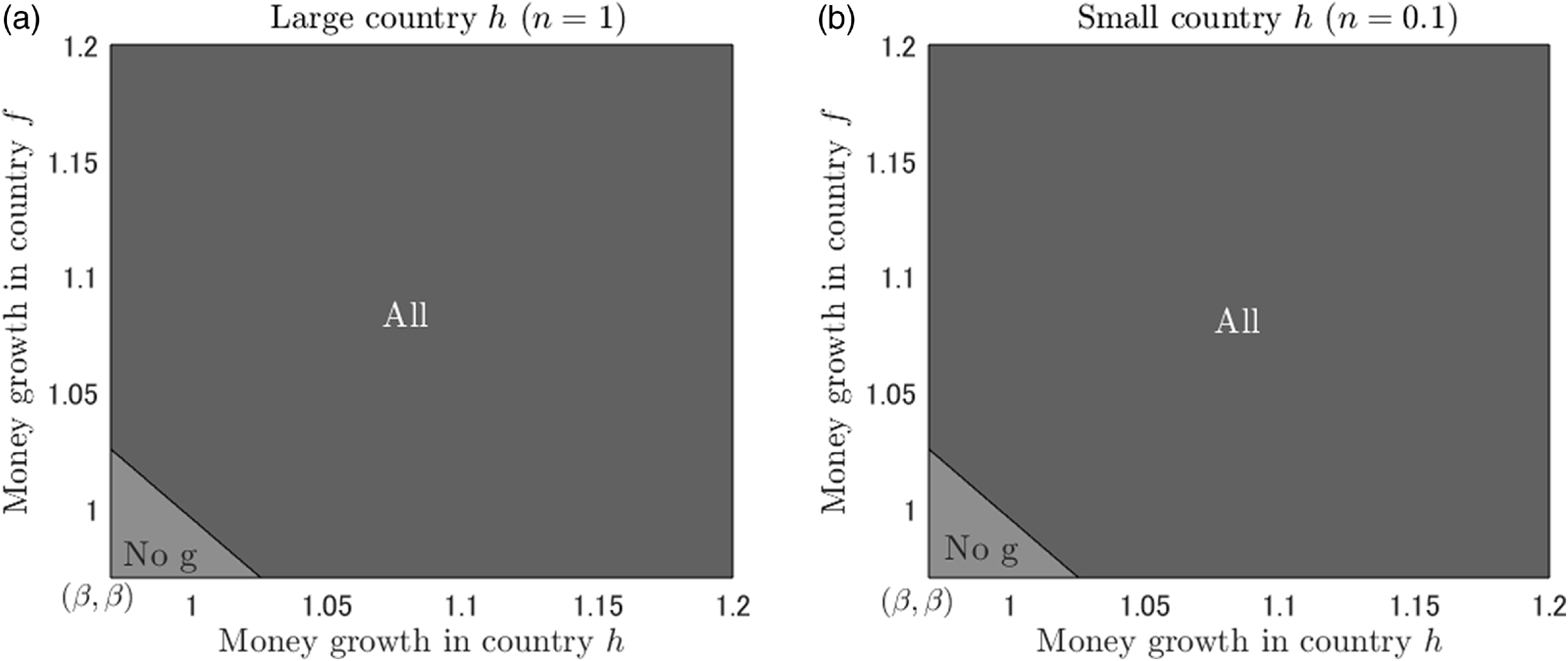Indeed, the presence of government sellers expands the region of a pair of $(\gamma _{h},\gamma _{f})$ in which all currencies are circulated, as shown in Figure 3.Footnote ¹⁶

Figure 3.

Monetary policy and international monetary system in the model with government sellers.

Note: ‘All’ indicates the circulation of all currencies. ‘No $\ell$ ’ indicates no circulation of currency $\ell \in \{h,f,g\}$ .

Unlike the baseline model (Figure 1) or the model with currency counterfeiting (Figure 2), the region of monetary autonomy remains unchanged with respect to the size of country $h$ . This is because the presence of government sellers ensures demand for national currencies, which eliminates the regions of no circulation of currency $h$ (‘No h’) or currency $f$ (‘No f’) in Figure 3.

Special case Consider a special case of $\alpha =1$ in which buyers are matched with sellers in the same country only. In this case, equations (40)–(42) are reduced to

(44) \begin{align}\frac {\gamma _{i}}{\beta }-1 = \mu _{ii}(1-\tilde {\mu }_{i}) \left [\! \frac {u^{\prime }\left ( c^{-1}(z_{i}^{i}+z_{i}^{\,g})\right )}{c^{\prime }\left (c^{-1}(z_{i}^{i}+z_{i}^{\,g})\right )}-1\right ]\! + \mu _{ii}\tilde {\mu }_{i}\left [\! \frac {u^{\prime }\left ( c^{-1}(z_{i}^{i})\right )}{c^{\prime }\left (c^{-1}(z_{i}^{i})\right )}-1\right ]\! \hspace {.5cm}\text{for $i\in \{h,f\}$}\end{align}

(45) \begin{align}\frac {\gamma _{g}}{\beta }-1 = \mu _{ii}(1-\tilde {\mu }_{i}) \left [\! \frac {u^{\prime }\left ( c^{-1}(z_{i}^{i}+z_{i}^{\,g})\right )}{c^{\prime }\left (c^{-1}(z_{i}^{i}+z_{i}^{\,g})\right )}-1\right ]\end{align}

Combining equations (44) and (45) yields

(46) \begin{equation} \frac {\gamma _{i}}{\beta }-\frac {\gamma _{g}}{\beta } = \mu _{ii}\tilde {\mu }_{i}\left [\! \frac {u^{\prime }\left ( c^{-1}(z_{i}^{i})\right )}{c^{\prime }\left (c^{-1}(z_{i}^{i})\right )}-1\right ]\! \end{equation}

If there is no government seller, $\tilde {\mu }_{i}=0$ , this condition is reduced to the equalization of the money growth rates as in Section 3.2.

Given that there are government sellers, $\tilde {\mu }_{i}\gt 0$ , and given that the growth rate of the national money is greater than that of the global money, $\gamma _{i}-\gamma _{g}\gt 0$ , the real balances of the national money is determined by equation (46). The total real balances of money, $z_{i} \equiv z_{i}^{i} + z_{i}^{\,g}$ , can be solved from equation (45). The solution constitutes an equilibrium in the global-money economy if $z_{i}^{\,g} = z_{i}-z_{i}^{i} \gt 0$ . From equations (45) and (46), this is the case if and only if

(47) \begin{equation} \gamma _{i} - \gamma _{g} \gt \frac {\tilde {\mu }_{i}(\gamma _{g} - \beta )}{1-\tilde {\mu }_{i}} \end{equation}

In the region that satisfies condition (47), monetary autonomy prevails in the global-money economy, which features the positive holdings of national and global money. Since the national money provides a greater liquidity service – the right-hand side of equation (44) – than the global money, in equilibrium the cost of holding the national money – the left-hand side of equation (44) – also has to be greater than the cost of holding the global money. Thus, the growth rate of the national money has to be high enough to satisfy condition (47) in the global-money economy.