VOTING RULES

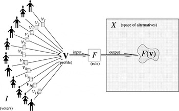
Let I represent a set of voters, and let V be the set of possible ‘votes’ (or ‘signals’ or ‘messages’) which could be sent by each voter. A profile is a list v which assigns a signal v _i in V to each voter i in I. Let V ^I denote the set of all possible profiles. Let X be a set of alternatives available to society (e.g. possible actions, possible answers to some question, job candidates). A voting rule is a correspondence F from V ^I to X – that is, for any profile v in V ^I, the rule yields a nonempty subset F(v)⊆X. Typically (but not always) F(v) will be a singleton. This is illustrated schematically in Figure 1.

Fig. 1.

A voting rule.

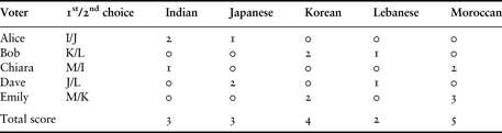
For example, suppose Alice, Bob, Chiara, Dave and Emily are trying to decide where to eat dinner. The available restaurants are Indian, Japanese, Korean, Lebanese, and Moroccan. (Thus, in this example, I = {Alice, Bob, Chiara, Dave, Emily}, while X = {Indian, Japanese, Korean, Lebanese, Moroccan}.) The five friends use the following rule: each person names her first choice and her second choice. (Thus, V = {I/J, I/K, I/L, I/M, J/I, J/K, J/L,…, M/L}, where, for example, ‘I/J’ represents a first choice of Indian and a second choice of Japanese.) A person's first choice gets two points, and her second choice gets one point – except for Emily. It is Emily's birthday, so her first choice gets three points, and her second choice gets two points. The restaurant which accumulates the most points wins. If the five friends vote as in Table 1, then the Moroccan restaurant wins with five points.

Table 1.

The restaurant problem

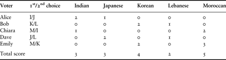
This is a simple example of a scoring rule. In a general scoring rule, there is a score function, S, which, for any voter i in I and any signal v in V, assigns a real-valued ‘score’ S(i,v,x) to each alternative x in X. (For example, in the restaurant voting rule, S(i, J/K, Japanese) = 2 and S(i, J/K, Korean) = 1 if i is any voter except Emily. Meanwhile S(Emily, J/K, Japanese) = 3 and S(Emily, J/K, Korean) = 2.) If there are N voters, then it will be convenient to represent the voters with the set I = {1,2,3,…,N}. (In the restaurant example, N = 5.) For any profile v in V ^I, let F _S(v) be the set of all element(s) x in X which maximize the sum S(1,v ₁,x) + S(2,v ₂,x) + … . + S(N,v _N,x). The resulting correspondence F _S from V ^I into X is the scoring rule defined by S. Many common voting rules can be represented as scoring rules. For example:

• • In the plurality rule, V = X, and, for every voter i in I, every alternative x in X, and every signal v in V, we have S(i,v,x) = 1 if v = x, whereas S(i,v,x) = 0 if v ≠ x. (Thus, each voter names her favourite choice. The alternative named by the most voters wins.)

• • In the weighted plurality rule, V = X, and, for every voter i in I, every alternative x in X, and every signal v in V, we have S(i,v,x) = w _i if v = x, whereas S(i,v,x) = 0 if v ≠ x. (Here, w _i is the ‘weight’ of voter i, which roughly measures her influence over the outcome.)

• • In the antiplurality rule, V = X, and for every voter i in I, every alternative x in X, and every signal v in V, we have S(i,v,x) = −1 if v = x, whereas S(i,v,x) = 0 if v ≠ x (i.e. each voter votes against her least-prefered alternative, implicitly endorsing all the other alternatives).

• • In approval voting, V is the set of all subsets of X, and, for every voter i in I, every alternative x in X, and any signal v in V (i.e. any subset v of X), we have S(i,v,x) = 1 if x is an element of v, whereas S(i,v,x) = 0 if x is not an element of v (Brams and Fishburn Reference Brams and Fishburn1983).

• • In range voting, V is the set of all functions mapping each element of X into a real number between 0 and 1, and, for every voter i in I, every alternative x in X, and every signal v in V, we have S(i,v,x) = v(x) (Smith Reference Smith2001).

• • In the Borda rule, V is the set of all preference orders over X, and, for every voter i in I, every alternative x in X, and every signal v in V, we have S(i,v,x) = r if x is ranked rth from the bottom according to the preference order v.

• • In the Kemeny (Reference Kemeny1959) rule, both V and X are the set of all preference orders over some set A of alternatives, and, for every voter i in I, every alternative x in X, and every signal v in V, the score S(i,v,x) is the number of pairwise comparisons on which the preference orders v and x agree.

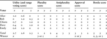
Table 2 illustrates the computation of the plurality, antiplurality, approval, Borda, and range voting rules. In this example, there are three alternatives, x, y and z, and five voters, Alice, Bob, Chiara, Dave and Emily. Each alternative has a utility for each voter which is between 0 and 1. We assume these utilities determine the outcome of the range voting rule, and we also assume that each voter ‘approves’ of an alternative if and only if it has a utility for her of at least 0.5. As shown in Table 2, different rules can produce different winners from the same profile.

Table 2.

Five scoring rules

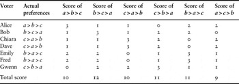
Next, Table 3 illustrates the Kemeny rule. We have three alternatives (say, A = {a,b,c}), so the space X contains six preference orders (i.e. X = {a > b > c, b > c > a, c > a > b, c > b > a, b > a > c, a > c > b}). This time, we suppose there are seven voters (say, I = {Alice, Bob, Chiara, Dave, Emily, Fred, Gwenn}). Each voter has a preference order over the alternatives. Each preference order on {a,b,c} is entirely described by three binary comparisons: a vs. b, b vs. c, and c vs. a. (For example, the preference order a > b > c corresponds to the assertions ‘a > b’, ‘b > c’, and ‘a > c’.) Thus, for any voter i in I, and any two preference orders x and v, the Kemeny score S(i,v,x) is 3 if v = x, and it is 0 if v is the exact reverse of x; otherwise it is either 1 or 2. The winning preference orderFootnote ⁸ is b > c > a, because it gets the highest total Kemeny score (namely, 12).

Table 3.

The Kemeny rule

Aside from the voting rule in the restaurant example and the weighted plurality rule, all of the scoring rules described above are anonymous, which means that every voter has exactly the same influence over the outcome as every other voter.Footnote ⁹ Also, the above rules are all neutral, which means that these rules do not favor any alternative in X over any other alternative.Footnote ¹⁰ If S(i,v,x) = −∞ for some voter i in I, some signal v in V, and some alternative x in X, then voter i can effectively ‘veto’ the choice x by sending the signal v. A rule has no vetos if this is never the case. All the above rules have no vetos.

STATISTICAL ESTIMATORS

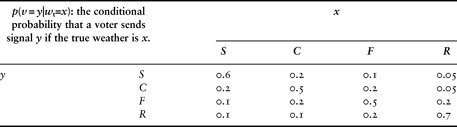
I will begin with an example. Suppose Alice, Bob and Chiara are three independent, equally competent meteorologists, who are trying to predict tomorrow's weather. For simplicity, suppose the weather can be in one of four states: Sunny, Cloudy, Foggy, or Raining. Assume that all three meteorologists have the predictive accuracy described in Table 4. For example, if the true state of tomorrow's weather is cloudy (C), then the C column of Table 4 says there is a 50% chance that a given meteorologist will correctly predict this fact, a 20% chance that she will incorrectly think it will be sunny (S), a 20% chance that she will incorrectly predict fog (F), and a 10% chance that she will incorrectly predict rain (R).

Table 4.

Predicting tomorrow's weather

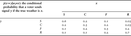
Another way to read Table 4 is in terms of likelihoods. If Alice predicts that it will be sunny, then the S row of Table 4 says that there is a 0.6 likelihood that this prediction is correct, a 0.2 likelihood that the weather will actually be cloudy, a 0.1 likelihood that it will be foggy, and a 0.05 likelihood of rain. (Likelihoods are not probabilities; observe that 0.6 + 0.2 + 0.1 + 0.05 ≠ 1.)

A profile is a list (v_a,v_b,v_c), summarizing the forecasts of the three meteorologists; we will denote it with the symbol v, as before. For example, suppose that Alice predicts that it will be sunny, Bob predicts that it will be cloudy, and Chiara predicts that it will be raining. Then, we have v _a = S, v _b = C, and v _c = R, yielding the profile v = (S,C,R).

Suppose tomorrow's weather will actually be sunny. Then, according to Table 4, the conditional probability that Alice predicts sunshine is given by p(v _a= S|w _t= S) = 0.6, while the conditional probability of Bob's prediction is p(v _b= C|w _t= S) = 0.2, and the conditional probability of Chiara's prediction is p(v _c= R|w _t= S) = 0.1. If Alice, Bob and Chiara make independent random errors, then the conditional probability of seeing the profile (S,C,R), given that tomorrow's weather is actually sunny, is the product of the conditional probabilities of their three individual predictions. In symbols: Prob[v = (S,C,R)|w _t= S] = p(v _a= S|w _t= S) × p(v _b= C|w _t= S) × p(v _c= R|w _t= S). More generally, the conditional probability of the profile (S,C,R) under the four possible weather states is as follows:Footnote ¹¹

(B1)

We refer to these values as the group likelihoods of the four states, given the profile (S,C,R).Footnote ¹² The maximum likelihood estimator, given the profile (S,C,R), is the state with the highest group likelihood. In this case, it is state S, which has a group likelihood of 0.012. Thus, if our only information about the weather was the forecasts of Alice, Bob and Chiara, then we would judge it more likely that tomorrow's weather will be sunny than that it will be any of the other three states. Thus, tomorrow might be a good day for a trip to the beach.

However, suppose that, based on historical data, we also know that the prior probability distribution of weather at this time of year is given by: Prob(S) = 0.2, Prob(C) = 0.4, Prob(F) = 0.2, and Prob(R) = 0.2. In that case, we compute the posterior probabilities of the four states as follows. First, define

(B2)

Now let R := R[S | S,C,R]+ R[C | S,C,R] +R[F | S,C,R] + R[R | S,C,R] = 0.00755. Then Bayes rule says that the posterior probabilities of the four states are as follows:Footnote ¹³

(B3)

The maximum a posteriori estimator, given this scenario and profile, is the state with the largest posterior probability. In this case, it is C, which attains a posterior probability of approximately 0.530. Perhaps tomorrow is not a good day for the beach, after all.

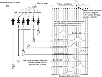
The example of the three meteorologists illustrates a much more general method. Suppose that X represents a set of possible ‘states of nature’. The true state is unknown. As before, let V be a set of possible ‘signals’ or ‘messages’ which could be sent by each voter. Suppose that each voter receives some partial information about the true state, which determines the way she votes. We can mathematically model these assumptions by specifying a prior probability distribution over X, and, for each voter i in I and every state x in X, specifying a probability distribution over V (called the error model), which describes the sort of signal which voter i is likely to send if the true state of nature is x. (In the example of the three meteorologists, we had V = X = {S,C,F, R}, and the error model was given by Table 4.) I will call a combination of a prior and an error model a scenario. I will say this scenario is anonymous if all voters are equally competent, and receive the same quantity and quality of information (i.e. for any state x in X, we have the same probability distribution over signals in V for every voter i in I). If the conditional probability of voter i sending signal v is zero, given state of nature x, then the scenario says certain events are ‘impossible’. If this never occurs, for any voter i in I, any signal v in V, and any state x in X, then I will say the scenario has no impossibilities. (For example, the error model in Table 4 is anonymous, and has no impossibilities.)

Assume that the signals sent by different voters are conditionally independent random variables, for any state of nature. (Informally, this means that each voter forms her opinion in isolation, without communicating with any of the other voters; thus, the errors she makes are not correlated with the errors of other voters.) Given any scenario Sc, and any profile v in V ^I, we can use Bayes rule to compute the posterior probability distribution over X, conditional on v. (In the meteorology example, this computation was performed in equations (B1), (B2), and (B3).) Let MAP(Sc,v) denote the element(s) of X which obtain maximal probability in this posterior distribution (the maximum a posteriori estimator determined by scenario Sc and profile v). This is the state which we deem to be most probable, given the information in the profile v, together with the background knowledge encoded in the scenario Sc. Thus, if we had to make a bet about the true state of nature, then our ‘best bet’ would be MAP(Sc,v). (In the meteorology example in Table 4, we had MAP(Sc,v) = {C}.) The computation of the maximum a posteriori estimator is schematically illustrated in Figure 2 above.

Fig. 2.

A maximum a posteriori estimator.

In particular, if we assume that the prior probability is uniformly distributed over X (i.e. all states are equally probable, a priori), then we obtain the maximum likelihood estimator determined by scenario Sc and profile v; this is denoted by MLE(Sc,v). This is the state which we deem to be most likely, given the information in the profile v, together with the voter error model encoded in the scenario Sc, but in the absence of any particular prior probability measure. (In the meteorology example in Table 4, we had MLE(Sc,v) = {S}.)

STATISTICAL RATIONALIZATION OF VOTING RULES

Let us say that a voting rule F is MAP-rationalizable if there is some error model (describing the fallibility of the voters' judgments) and some a priori probability distribution on X (describing our prior knowledge of the situation) such that, for any profile v of signals from the voters, the outcome F(v) is the maximum a posteriori estimator in X, given the data in v, according to this error model and prior distribution.Footnote ¹⁴ In other words, the decisions made by F can always be ‘rationalized’ as the outcome of a statistical procedure, based on some scenario describing the information available to the voters.

Let us say that the rule F is MLE-rationalizable if this rationalization can be made with a uniformly distributed prior probability distribution. This means that there is some error model (describing the fallibility of the voters) such that, for any profile v of signals, the rule F computes the maximum likelihood estimator in X, given the data in v. Finally, let us say that the rule F is anonymously MAP-rationalizable if the rationalizing error model is anonymous. Pivato (Reference Pivato2012) proves the following result.

In particular, this theorem implies that the (anti)plurality, Borda, Kemeny, approval, and range-voting rules are all anonymously MLE-rationalizable. The restaurant voting rule (Table 1) and the weighted plurality rule are (non-anonymously) MLE-rationalizable. Thus, the application of each of these voting rules to epistemic social decisions can be justified by positing a suitable error model, describing the fallibility of the voters. (Of course, sometimes this error model is not very plausible.)

If a voting rule cannot be represented as a scoring rule, then the Rationalization Theorem tells us that it cannot be MAP-rationalized. But some voting rules which do not initially look like scoring rules might admit some obscure scoring representation. Thus, the Rationalization Theorem is not very useful unless there is a simple way to determine whether a voting rule is a scoring rule. One way is to look for a property called reinforcement. A voting rule F satisfies this property if the following is true: given two disjoint populations, if each of these populations, in isolation, selects an alternative x when it uses the rule F, then the combined population should also select the alternative x when it uses the rule F. All scoring rules satisfy reinforcement. (Indeed, results of Myerson (Reference Myerson1995) and Pivato (Reference Pivato2011) imply that, amongst neutral voting rules, scoring rules are essentially the only rules which satisfy reinforcement.) Thus, a rule which violates reinforcement cannot be MAP-rationalizable. This eliminates many popular voting rules, such as plurality vote with runoff (used in the French presidential election), instant runoff (used in the Irish and Indian presidential elections), successive elimination rules (used in many sports tournaments, and also used by the US Congress to decide between a bill and its amendments), the Copeland rule (choose the alternative which beats the most other alternatives in a two-way vote), the Simpson-Kramer rule (choose the alternative with the smallest majority opposing it in a two-way vote), the Schulze rule, and the Slater rule. This makes it very hard to defend the use of any of these voting rules in an epistemic context.

METRIC VOTING RULES AND METRIC ERROR MODELS

The fact that a voting rule can be rationalized by some scenario does not imply that this scenario is a particularly realistic description of the epistemic problem facing society. What would a realistic description look like? Typically, the space X of alternatives has a sort of ‘geometry’; there is a sense in which some elements of X are ‘close together’ (i.e. very similar), whereas other elements are ‘far apart’ (very dissimilar).Footnote ¹⁶ Suppose each voter's signal is a guess about the correct element in X (so in this model, V = X). If the voters are not completely unreliable, then they are more likely to guess an answer which is close to the right answer than one which is far away.

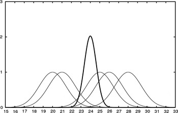
For example, suppose five fallible, but independent and equally competent meteorologists want to predict tomorrow's temperature. Alice predicts a temperature of 20 degrees Celsius, Bob predicts 21 degrees, Chiara predicts 25 degrees, Dave predicts 26 degrees, and Emily predicts 28 degrees. Suppose each meteorologist's prediction is the true temperature, plus a random error. Suppose these errors are independent, identically distributed normal (i.e. Gaussian) random variables.Footnote ¹⁷ Then the maximum likelihood temperature, given the profile (20,21,25,26,28), is 24 degrees – the mean of the five estimates. In Figure 3, the (Gaussian) likelihood functions of the five meteorologists are the five smaller thin curves. The thick curve is product of these five functions (rescaled); it is the group likelihood function. Note that it obtains its maximum at 24. Note also that the group likelihood function has a much narrower peak than the individual likelihood functions. In other words, it has a smaller variance, indicating a greater degree of certainty. Indeed, if we had aggregated the estimates from a larger group of (equally competent, statistically independent) meteorologists, then the variance would be even smaller (indicating even greater certainty). In fact, the variance approaches zero (perfect certainty) as the number of meteorologists grows to infinity. This illustrates the wisdom of crowds effect, first observed by Galton (Reference Galton1907), and recently popularized by Surowiecki (Reference Surowiecki2004).

Fig. 3.

Predicting tomorrow's temperature with Gaussian random errors.

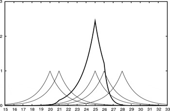
Now suppose instead that the meteorologists' errors are independent, identically distributed exponential random variables.Footnote ¹⁸ Then the maximum likelihood estimator is 25 degrees – the median of the five estimates. In Figure 4, the (exponential) likelihood functions of the five meteorologists are the five thin curves. The thick curve is product of these five functions (rescaled); it is the group likelihood function. Note that it obtains its maximum at 25.

Fig. 4.

Predicting tomorrow's temperature with exponential random errors.

In both of these examples, the meteorologists' mistakes were described by a metric error model. Formally, this means that, for every voter i in I, there is a (decreasing) real-valued function E _i such that, if the true state is x, then for any other state v in X, the probability that voter i guesses v is given by E _i[d(x,v)], where d(x,v) is the ‘distance’ between x and v in X.Footnote ¹⁹ Metric error models seem quite plausible; they capture the idea that reasonably competent voters are less likely to make large errors than small errors. If the space X of states of nature has a natural geometric structure (e.g. a temperature scale), then almost any reasonable explanation of how the voters make their mistakes will result in a metric error model.

In both the temperature examples, the MLE can be described as the outcome of a scoring rule. In the Gaussian error model, the score function is given by S(i,v,x)= −(v−x)², for every meteorologist i and all possible temperatures v and x. (For example, S(i, 22, 25) = −3² = −9.) In the exponential error model, the score function is given by S(i,v,x) = −|v−x|, for every meteorologist i and all possible temperatures v and x. (For example, S(i, 22, 25) = −|22−25| = −3.) Note that, in both cases, S(i,v,x) depends only on the distance between v and x; furthermore, the score decreases as the distance increases. A scoring rule with this structure is called a metric voting rule: for each voter i in I and all states x and v in X, the value of S(i,v,x) is a decreasing function of the distance between v and x. (In both temperature examples, the score function was anonymous, but this need not be the case in general.)

These examples illustrate a general pattern: the MLE or MAP for any metric error model is a metric voting rule. Conversely, any metric voting rule can be MAP-rationalized in terms of a metric error model. Thus, the Rationalization Theorem becomes much more plausible and compelling in the setting of metric voting rules.

In particular, suppose, in the metric error model, that the functions E _i are exponentially decaying for all voters i in I.Footnote ²⁰ Then it can be shown that (for a suitable prior probability distribution) the MAP estimator is the weighted median rule. Footnote ²¹ For any profile v, the weighted median rule picks the element(s) of X which minimize the sum w ₁d(x,v ₁) + w ₂d(x,v ₂) + …+ w _Nd(x,v _N), where w ₁,w ₂,…,w _N are nonnegative ‘weights’ assigned to the voters. In other words, the weighted median rule chooses the state in X which has the smallest weighted average distance to the opinions of the voters. The rule is anonymous (i.e. treats all voters the same) if and only if w ₁= w ₂= …= w _N = 1;Footnote ²² this yields the (unweighted) median rule, which minimizes the sum d(x,v ₁) + …+ d(x,v _N). (Thus, the median rule chooses the state in X which has the smallest average distance to the opinions of the voters.) The temperature estimation example in Figure 4 illustrated the median rule on the set ℝ of all real numbers (i.e. all possible temperatures). A space X is called homogeneous if the geometry of X ‘looks the same’ around each alternative x in X.Footnote ²³ For example, the space ℝ is homogeneous. In this case, as we saw above, the median rule is the MLE for any anonymous exponential error model.Footnote ²⁴

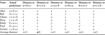
For another example, let X be the space of all strict preference orders on some set A of alternatives. For any x and y in X, let d(x,y) be the number of pairs in A on which the orders of x and y disagree. Then the structure described by X and d is a homogeneous space. The median rule on X is the Kemeny rule. To illustrate this, consider a set of three alternatives (i.e. A = {a,b,c}). Recall that each preference order on {a,b,c} is entirely described by three binary comparisons: a vs. b, b vs. c, and c vs. a. Thus, for any two preference orders x and y, we have d(x,y) = 0 if x = y, while d(x,y) = 3 if x is the exact reverse of y; otherwise d(x,y) = 1 or 2. Table 5 portrays the same seven-voter profile which I earlier used to illustrate the Kemeny rule in Table 3. The median preference order is b > c > a, which attains the smallest average distance (of 9/7) to the preferences of the voters. Observe that this agrees with the output of the Kemeny rule, which we computed in Table 3.

Table 5.

The Kemeny rule as a median rule

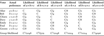
The space X of all preference orders is homogeneous. Thus, the Kemeny (i.e. median) rule is the MLE for any anonymous exponential error model on X; this was first noted by Young (Reference Young, Grofman and Owen1986, Reference Young1988, Reference Young1995, Reference Young and Mueller1997).Footnote ²⁵ For example, consider an exponential error model on these preference orders, such that, if the true preference order is x, then the probability of a voter choosing preference order v is given by p(v|x) = C (½)^d(v,x) (where C = 8/21).Footnote ²⁶ For the seven-voter profile above, the likelihoods are given by Table 6. The maximum likelihood preference order is b > c > a, which attains a likelihood of C ⁷/512. Observe that this agrees with the output of median and the Kemeny rule.Footnote ²⁷

Table 6.

The Kemeny rule as a maximum likelihood estimator

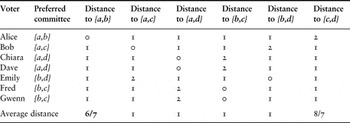
Here is another example. Suppose we must pick a committee with two members from a set of four candidates: a, b, c, and d. Let V and X both be the set of all admissible committees; that is, V = X = { {a,b}, {a,c}, {a,d}, {b,c}, {b,d}, {c,d} }. For any two committees x and y in X, let d(x,y) be the number of members on which they disagree (for example, d({a,b},{b,c}) = 1). Consider the seven-voter profile described by Table 7. The median committee is {a,b}, which attains the minimal average distance (of 6/7) to the preferred committees of the voters.

Table 7.

The median rule for committee selection

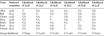
Now suppose there is some committee which is truly the best choice. Consider an exponential error model such that, if x is truly the best committee, then the probability of a voter choosing the committee v is given by p(v|x) = C (⅓)^d(v,x) (where C = 9/46).Footnote ²⁸ For the seven-voter profile above, the likelihoods are shown in Table 8. The maximum likelihood committee is {a,b}, which attains a likelihood of C ⁷/729. Note that this agrees with the outcome of the median rule, computed in Table 7.

Table 8.

The MLE committee selection

This example illustrates a more general pattern. Let A be a set of possible candidates for some committee. (In Tables 6 and 7, we had A = {a,b,c,d}.) Let X be the set of all committees comprised of exactly n of these candidates (for some fixed n ≤ |A|). For any two committees x and y in X, let d(x,y) be the number of candidates on which the committees x and y disagree. Then the structure described by X and d is a homogeneous space. Thus, the median rule is the MLE for any anonymous exponential error model on X.Footnote ²⁹

An MLE rationalization of the median rule is only valid if X is homogeneous in the sense described above. But most metric spaces are not homogeneous. On inhomogeneous spaces, the median rule can still be MAP-rationalized, but the prior probability distribution will generally not be uniform. For instance, in the temperature-prediction example, it is unrealistic to suppose that the temperature could be any real number. It certainly must be greater than −100 degrees Celsius (at which temperature carbon dioxide would freeze and snow out of the atmosphere). Furthermore, it is most likely less than 100 degrees Celsius on the surface of the earth (except perhaps near intense geothermal activity). So perhaps we should let X be the interval of all real numbers between −100 and 100. But this interval is not homogeneous, so if we did this, then the median rule would no longer be MLE-rationalizable. If the number of voters was relatively small, and their predictions were far from the boundaries of the interval (as was the case in our example), then the deviation from a uniform prior probability distribution would be very small, so the median would still agree with the MLE almost all the time. However, as the number of voters becomes large, the rationalizing prior probability distribution will become increasingly concentrated near the exact center of the interval (which is 0 degrees, in this case). In this case, the median temperature estimate will often deviate from the maximum likelihood estimator.Footnote ³⁰

For another example, consider the set of all committees containing at least two members and at most four members, drawn from a set of ten possible candidates. Unlike the committee space we considered in Tables 6 and 7, this committee space is not homogeneous. The median rule on this space is MAP-rationalizable (with a non-uniform prior probability distribution), but it is not MLE-rationalizable.Footnote ³¹

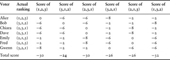
The Borda rule is another metric voting rule with an interesting statistical rationalization. To illustrate this, let A = {a,b,c} be a set of three alternatives, and consider the seven-voter profile of preferences we used in Tables 3, 5 and 6 to illustrate the Kemeny rule. Table 9 shows the same profile, with the voters' preference orders represented as ranking vectors of {a,b,c}; that is, three-dimensional vectors (r _a, r _b, r _c), such that, for all n in {1,2,3}, there is exactly one element x in {a,b,c} such that r _x = n. (Lower ranks are better.) For every voter i in I, every signal y in X, and every alternative x in X, let S(i,y,x): = −|x−y| ²; then the resulting scoring rule is a metric voting rule, because the score function S(i,y,x) only depends on the Euclidean distance from x to y.Footnote ³² In fact, this scoring rule is the Borda rule, expressed in terms of ranking vectors. In the example in Table 9, the Borda rule chooses the ranking vector (3,1,2), which achieves the maximal score (namely −24). This corresponds to the preference order b > c > a.

Table 9.

The Borda rule as a metric voting rule (metric error model on ranking vectors)

Now suppose that one ranking of the set {a,b,c} is the ‘true’ ranking. Consider an error model such that, if x is truly the best ranking, then the probability of a voter choosing the ranking v is given by p(v|x) = C exp(−|v−x| ²) (where C is a constant).Footnote ³³ For the seven-voter profile in Table 9, the likelihoods are given by Table 10. The correspondence with the Table 9 is obvious. The last row of Table 10 shows the group likelihoods of the six possible preference orders in X, which are obtained by multiplying the likelihoods from the seven previous rows.Footnote ³⁴ The maximum likelihood ranking is again (3,1,2), in agreement with the Borda ranking.Footnote ³⁵

Table 10.

The Borda rule as an MLE (Gaussian error model on ranking vectors)

This example illustrates a much more general pattern, which can be seen as a generalization of the earlier temperature prediction example with Gaussian errors (Figure 3). Let M be a positive integer, and let X be any homogeneous subset of M-dimensional Euclidean space (i.e. ℝ^M), which we endow with the standard Euclidean notion of distance. (In the temperature estimation example in Figure 3, we had M = 1 and X = ℝ; in Table 10, we have M = 3 and X = {(1,2,3), (3,1,2), …, (3,2,1)}.) Consider an anonymous Gaussian error model on X.Footnote ³⁶ The MLE for this error model is the metric voting rule where S(i,y,x) = −|x−y| ² for every voter i in I, every signal y in X, and every alternative x in X. Footnote ³⁷ In this case, maximizing the total score is equivalent to minimizing the mean squared distance to the votes sent by the voters. It is easy to checkFootnote ³⁸ that this scoring rule simply chooses the element(s) of X which are closest to the average of the signals v ₁,v ₂,…,v _N, when treated as M-dimensional vectors in ℝ^M.Footnote ³⁹

In particular, let A be a set of M social alternatives. A ranking vector of A is an M-dimensional vector r (with co-ordinates indexed by the elements of A) such that, for all m in {1,2,…,M}, there is exactly one element a in A such that r _a = m. (Lower ranks are better.) We can regard r as a vector in the M-dimensional Euclidean space ℝ^M. Let X be the set of all such ranking vectors; then X is a subset of ℝ^M. Then X is homogeneous, and the averaging rule (i.e. the MLE for any Gaussian error model) is the Borda rule, as we saw in the example from Tables 9 and 10 (where A = {a,b,c}, so that M = 3). This argument provides another MLE-rationalization for the Borda rule, which is quite different from the rationalization given by Young (Reference Young, Grofman and Owen1986). Variations of this setup yield MLE-rationalizations of other ‘ranking’ rules, including the plurality rule and anti-plurality rule portrayed in Table 2.

RATIONALIZING VOTING RULES AS EXPECTED UTILITY MAXIMIZERS

Now let us turn to the problem of expected utility maximization. Many voting rules invite each voter to assign a numerical ‘score’ to each social alternative. Then the rule chooses the alternative with the highest average score. Rules differ on what range of scores are admissible. For example:

• • Classical utilitarianism allows the score of an alternative to be any real number.

• • Range voting allows the score of an alternative to be any real number between 0 and 1.

• • Approval voting requires the score of each alternative to be either 0 or 1.

In all of these rules, a voter can give the same score to two or more alternatives (unlike the Borda rule, (anti)plurality rule, and other ‘ranking’ rules). I will refer to rules with this property as quasiutilitarian.

Any quasiutilitarian voting rule can be rationalized as an expected utility maximizer. Suppose that the score a voter assigns to an alternative reflects her (possibly inaccurate) estimate of the ‘social utility’ of that alternative. Although the voters' estimates may be incorrect, we can assume that they are not totally perverse: under reasonable assumptions about the voters' (mis)perceptions, one can show that, if alternative a receives an average score of r, and alternative b receives an average score of s, and r > s, then the conditionally expected utility of a, given this information, is higher than the conditionally expected utility of b. (This does not mean that r itself is a good estimate of the expected utility of a – but this isn't necessary.) I will say an error model with this property is regular. It is easy to see that a quasiutilitarian rule is an expected utility maximizer for any regular error model. In particular, this yields EUM-rationalizations of classical utilitarianism, range voting, approval voting, and a ‘relaxed’ version of the Borda rule (where a voter can give the same rank to two or more alternatives).Footnote ⁴⁰

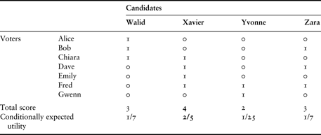
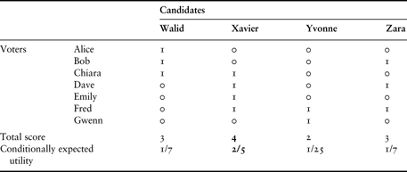
For example, consider a hiring committee which must choose one of four candidates for a position. The four candidates are Walid, Xavier, Yvonne and Zara (so X = {w,x,y,z}). The hiring committee is the same seven voters who have appeared in previous examples. Suppose each candidate is either competent to do the job, or incompetent – there are no finer gradations of skill. Hiring a competent candidate yields a utility of 1; hiring an incompetent candidate yields a utility of 0. The hiring committee simply wants to maximize its expected utility – or equivalently, maximize the probability that it hires a competent candidate. Each voter makes a private estimate of the competency of each candidate: either 1 if she thinks the candidate is competent, or 0 if she thinks he is incompetent. Suppose this estimate is correct with probability ⅔, and incorrect with probability ⅓. We also suppose the true competencies of the candidates are independent, identically distributed random variables. To be concrete, suppose each candidate is competent with probability ¼, and incompetent with probability ¾.

Consider the profile of voter opinions described by Table 11. (For example, in this profile, Alice believes that Walid is competent, but she believes that the other three candidates are incompetent.) In the second-last line of Table 11, we have summed up the scores for each candidate. In effect, this is each candidate's score in the approval voting procedure. Observe that Xavier is the winner of the approval voting procedure, attaining a score of 4. In the last line of Table 11, we have also computed the conditionally expected utility for each candidate, given the opinions of the voters and based on the scenario we described above. Equivalently, this is the conditional probability that each candidate is competent. (The details of this computation are omitted.) Xavier is competent with probability 2/5, which is much higher than the competency probability of any other candidate. Thus, hiring Xavier will maximize expected utility. This illustrates a general pattern: in hiring problems of this kind, the approval voting procedure will always chose the candidate who yields the maximal expected utility.Footnote ⁴¹

Table 11.

The hiring problem (approval voting as an expected utility maximizer)

If we suppose that the competency of each candidate can be any value between 0 and 1, then we can obtain a very similar EUM interpretation of range voting instead of approval voting. We can likewise interpret the classic utilitarian rule as an expected utility maximizer. Unlike the Rationalization Theorem, these results do not depend upon a specific choice of error model; they are true for any ‘regular’ error model, as defined above. Thus, under quite plausible conditions, these rules will maximize the expected level of social utility. This provides a very strong argument for using these rules in social decision problems where the group agrees on an underlying utility function, but is uncertain about the best course of action.