

1 Introduction
This paper considers the response of premixed flames to helical flow disturbances. Helical flow disturbances are common in circular shear flows. In the case of non-swirling round jets, theory predicts that the strength of the axisymmetric,  $m_{u}=0$ mode relative to that of the low-order helical modes (
 $m_{u}\neq 0$) depends on the boundary layer thickness relative the jet radius (Michalke Reference Michalke1984). Helical modes dominate the region downstream of the potential core (Liepmann & Gharib Reference Liepmann and Gharib1992). Similarly, for axisymmetric non-swirling wakes, it is the helical
 $m_{u}=\pm 1$ modes that dominate the flow dynamics (Pier Reference Pier2008). Swirling jets are generally dominated by helical disturbances (Fick, Griffiths & O’Doherty Reference Fick, Griffiths and O’Doherty1997; Cala et al. Reference Cala, Fernandes, Heitor and Shtork2006; Jochmann et al. Reference Jochmann, Sinigersky, Hehle, Schäfer, Koch and Bauer2006; Syred Reference Syred2006; Shtork, Vieira & Fernandes Reference Shtork, Vieira and Fernandes2008; Huang & Yang Reference Huang and Yang2009; Oberleithner et al. Reference Oberleithner, Sieber, Nayeri, Paschereit, Petz, Hege, Noack and Wygnanski2011; Meliga, Gallaire & Chomaz Reference Meliga, Gallaire and Chomaz2012; Tammisola & Juniper Reference Tammisola and Juniper2016). The presence of swirl introduces shear in the azimuthal direction and an additional instability mechanism due to the Rayleigh centrifugal instability criterion. Swirl also biases the strength of the helical modes; i.e. the growth rates of the
 $m_{u}>0$ (positive) and corresponding
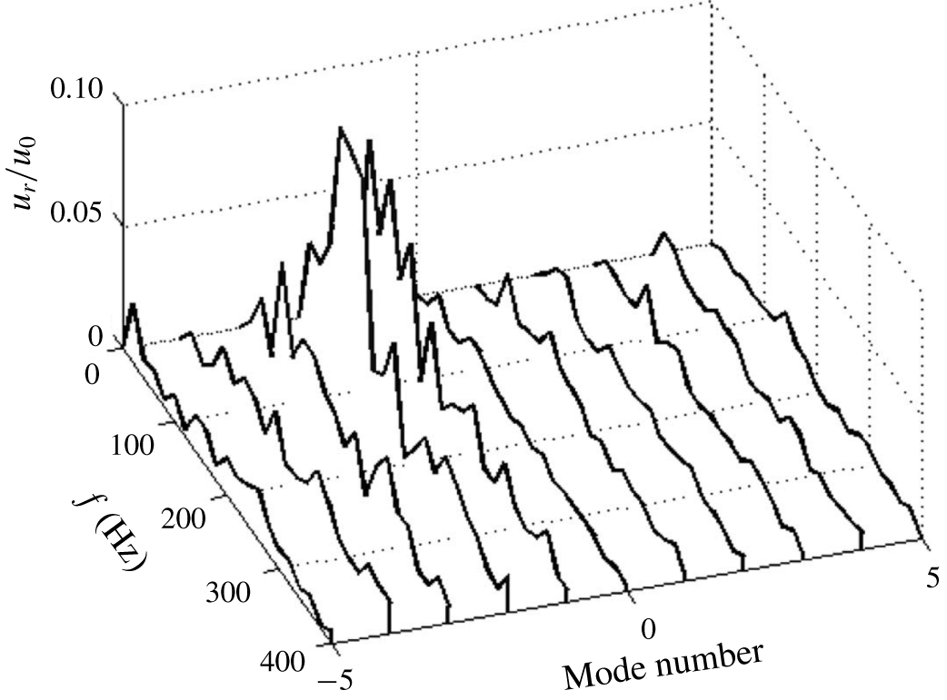
 $m_{u}<0$ (negative) modes are different. This is evident from the amplitude distribution for different helical modes as shown in the experimental data reproduced in figure 1. Note that the largest energy content in the flow is in the modes,
 $m_{ur}=-1,-2$, which are substantially larger than the
 $m_{ur}=0,+1$ or
 $+2$ modes.
Frequency spectrum showing helical mode amplitude variation of different helical modes from a swirling flow experiment. Figure reproduced from O’Connor & Lieuwen (Reference O’Connor and Lieuwen2012).

This paper will use the following notation for the perturbation decomposition. The velocity field can be decomposed into an unperturbed (subscript ‘0’) and a spatio-temporally varying disturbance (subscript ‘1’ for linear first order), as
 $$\begin{eqnarray}u_{j}(r,\unicode[STIX]{x1D703},z,t)=u_{j,0}(r,\unicode[STIX]{x1D703},z)+\unicode[STIX]{x1D716}u_{j,1}(r,\unicode[STIX]{x1D703},z,t),\end{eqnarray}$$
where the subscript  $j$ denotes the
 $r$,
 $\unicode[STIX]{x1D703}$ or
 $z$ coordinate. For discrete frequencies contained in this velocity, the velocity field can be decomposed into its frequency domain components as
 $$\begin{eqnarray}u_{j,1}(r,\unicode[STIX]{x1D703},z,t)=\mathop{\sum }_{n=0}^{N}\hat{u} _{j,1}(r,\unicode[STIX]{x1D703},z,\unicode[STIX]{x1D714}_{n})\text{e}^{-\text{i}\unicode[STIX]{x1D714}_{n}t}.\end{eqnarray}$$
The overhat denotes the complex frequency domain component of the velocity at frequency  $\unicode[STIX]{x1D714}_{n}$. The complex velocity is also decomposed spatially into helical modes as
 $$\begin{eqnarray}\hat{B}_{j,m_{uj}}(r,z,\unicode[STIX]{x1D714})=\int _{\unicode[STIX]{x1D703}=0}^{2\unicode[STIX]{x03C0}}\text{e}^{-\text{i}m_{uj}\unicode[STIX]{x1D703}}\hat{u} _{j,1}(r,\unicode[STIX]{x1D703},z,\unicode[STIX]{x1D714})\,\text{d}\unicode[STIX]{x1D703}.\end{eqnarray}$$
Here,  $\hat{B}_{j,m_{uj}}$ is the complex modal coefficient corresponding to flow helical mode number
 $m_{uj}$ in the flow component along the
 $j$ direction. Going forward, different subscripts for the mode numbers shall be used to differentiate between mode numbers in the flow disturbance asymmetries,
 $m_{uj}$, flame disturbance asymmetries,
 $m_{\unicode[STIX]{x1D709}k}$, and time-averaged flame asymmetries,
 $m_{\unicode[STIX]{x1D709}_{0}}$. The helical mode numbers are signed integers and thus, we have
 $$\begin{eqnarray}\hat{u} _{j,1}(r,\unicode[STIX]{x1D703},z,\unicode[STIX]{x1D714})=\mathop{\sum }_{m_{uj}=-\infty }^{+\infty }\hat{B}_{j,m_{uj}}(r,z,\unicode[STIX]{x1D714})\text{e}^{\text{i}m_{uj}\unicode[STIX]{x1D703}}.\end{eqnarray}$$
Note that  $m_{uj}=0$ is the axisymmetric mode. To understand the sign of the asymmetric helical mode, consider the phase function of the disturbance at a fixed time, defined as
 $(-\unicode[STIX]{x1D714}t+m_{uj}\unicode[STIX]{x1D703})$, where
 $\unicode[STIX]{x1D703}$ increases in the swirl direction. Hence, defining the rotation direction of the flow to be in the increasing
 $\unicode[STIX]{x1D703}$ direction, a positive mode
 $m_{uj}>0$ has a line of constant phase in the swirl direction. Conversely, a negative mode
 $m_{uj}<0$ is counter-rotating with the swirl. As noted above, the positive and negative modes are amplified differently, and also interact very differently with the flame as shown in earlier linear analysis (Acharya, Shin & Lieuwen Reference Acharya, Shin and Lieuwen2013). Flames are often stabilized in regions of lower flow velocity and high shear, and are strongly disturbed by the natural or forced flow disturbances in the shear layer. This disturbance of the flame leads to unsteady heat release rate oscillations. These oscillations also generate sound, i.e. combustion generated noise (Dowling & Stow Reference Dowling, Stow, Lieuwen and Yang2005; Hirsch et al. Reference Hirsch, Wäsle, Winkler and Sattelmayer2007; Candel et al. Reference Candel, Durox, Ducruix, Birbaud, Noiray and Schuller2009; Rajaram & Lieuwen Reference Rajaram and Lieuwen2009), as well as close the loop in the thermoacoustic feedback (Lieuwen Reference Lieuwen2012).
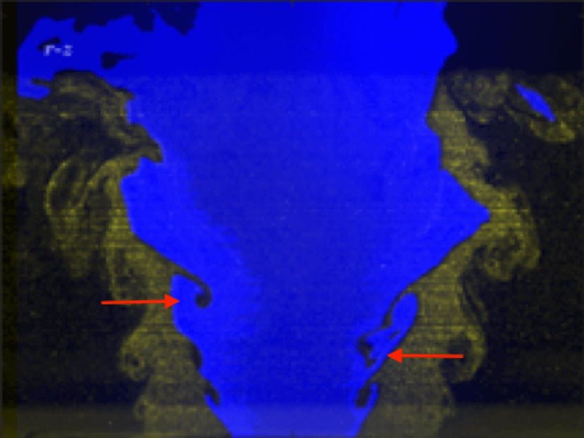
Sample instantaneous image showing helical disturbances (red arrows indicate roll-up), showing alternating vortical roll-up of flame surface. Yellow is Mie scattering from the flow and blue is OH-PLIF (Smith et al. Reference Smith, Emerson, Proscia and Lieuwen2018).
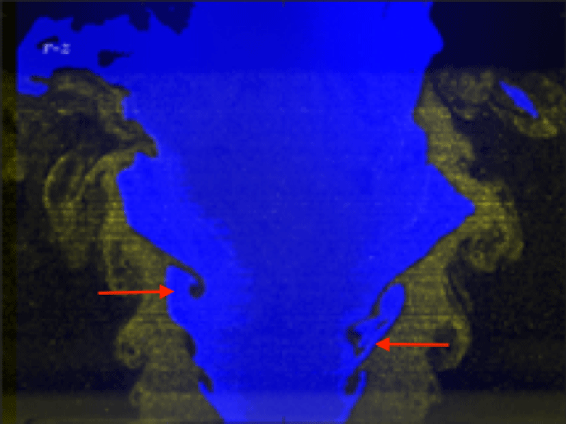
Several studies of forced, swirl flames have detailed the presence of helical disturbances on the flame (Paschereit, Gutmark & Weisenstein Reference Paschereit, Gutmark and Weisenstein2000; Lacarelle et al. Reference Lacarelle, Faustmann, Greenblatt, Paschereit, Lehmann, Luchtenburg and Noack2009). The helical disturbances introduce wrinkles on the flame (see figure 2) that are convected axially and azimuthally due to the presence of swirl, introducing both axial and azimuthal phase variations in local unsteady heat release rate oscillations (Bellows et al. Reference Bellows, Bobba, Forte, Seitzman and Lieuwen2007; Thumuluru & Lieuwen Reference Thumuluru and Lieuwen2009). For similar reasons, co- and counter-rotating helical modes affect the flame in different ways in the presence of swirl. Experiments have shown helical modes exciting azimuthally rotating unsteady heat release rate oscillations on the flame (Moeck et al. Reference Moeck, Bourgouin, Durox, Schuller and Candel2012; Stöhr et al. Reference Stöhr, Boxx, Carter and Meier2012). In addition, experiments in an annular combustor with multiple nozzles analysed the global flame dynamics during self-excited circumferential instabilities (Worth & Dawson Reference Worth and Dawson2013). In this combustor, the azimuthal location of the nozzles in the standing wave is important, as different helical disturbances are excited at different locations in the acoustic standing wave and, thus, cause differing flame response (Worth & Dawson Reference Worth and Dawson2013; O’Connor, Acharya & Lieuwen Reference O’Connor, Acharya and Lieuwen2015). However, the flames excited by helical disturbances had much smaller amplitude of unsteady heat release rate oscillations relative to those excited by axisymmetric structures, for reasons discussed later. A significant number of experiments have characterized the response of flames to forced excitation with varying amplitude, to characterize this sensitivity in both the linear and nonlinear regime (Külsheimer & Büchner Reference Külsheimer and Büchner2002; Lee & Santavicca Reference Lee and Santavicca2003; Balachandran et al. Reference Balachandran, Ayoola, Kaminski, Dowling and Mastorakos2005; Armitage et al. Reference Armitage, Balachandran, Mastorakos and Cant2006; Bellows et al. Reference Bellows, Bobba, Forte, Seitzman and Lieuwen2007; Noiray et al. Reference Noiray, Durox, Schuller and Candel2008; Durox et al. Reference Durox, Schuller, Noiray and Candel2009; Karimi et al. Reference Karimi, Brear, Jin and Monty2009; Schimek, Moeck & Paschereit Reference Schimek, Moeck and Paschereit2011), nonlinear studies have shown that the nonlinearities in flame response to large scale vortical structures arises from both fluid mechanic (i.e. saturation in response of vortical disturbances, (Terhaar, Oberleithner & Paschereit Reference Terhaar, Oberleithner and Paschereit2014; Oberleithner, Schimek & Paschereit Reference Oberleithner, Schimek and Paschereit2015), as well as kinematic restoration processes (Bellows et al. Reference Bellows, Bobba, Forte, Seitzman and Lieuwen2007).
The response of premixed flames to hydrodynamic flow disturbances has also been considered theoretically. These models focused on both the local flame response (local wrinkling amplitude and phase, local unsteady heat release rate oscillations), as well as the global flame response through the spatially integrated unsteady heat release rate oscillations. The local unsteady heat release rate oscillations per unit area of a premixed flame is given by
 $$\begin{eqnarray}\dot{q}=\unicode[STIX]{x1D70C}_{u}s_{L}h_{R}.\end{eqnarray}$$
Here,  $\unicode[STIX]{x1D70C}_{u}$ is the unburnt reactant density,
 $s_{L}$ is the flame speed and
 $h_{R}$ is the heat of reaction. For acoustically compact flames it is the spatially integrated ‘global’ unsteady heat release rate oscillations,
 $\dot{Q}(t)$, that controls the noise generation by flames and/or the thermoacoustic stability of a ducted system. This global unsteady heat release rate oscillations is given by
 $$\begin{eqnarray}\dot{Q}(t)=\int _{flame}\unicode[STIX]{x1D70C}_{u}s_{L}h_{R}\,\text{d}A.\end{eqnarray}$$
The global unsteady heat release rate oscillations can be decomposed about its time average and fluctuation as
 $$\begin{eqnarray}\dot{Q}(t)=\bar{\dot{Q}}+\dot{Q}^{\prime }(t).\end{eqnarray}$$
The sensitivity of  $\dot{Q}^{\prime }(t)$ to helical flow disturbances is the key focus of this paper, quantified via the flame describing function,
 $\text{FDF}$. This function is an amplitude dependent quantity that denotes the nonlinear response of global unsteady heat release rate oscillations to input flow fluctuations at a given frequency and amplitude. The
 $\text{FDF}$ is defined as
 $$\begin{eqnarray}\text{FDF}(\unicode[STIX]{x1D714},\unicode[STIX]{x1D716})=\frac{\hat{\dot{Q}}^{\prime }(\unicode[STIX]{x1D714},\unicode[STIX]{x1D716})/\bar{\dot{Q}}}{\hat{u} _{ref}^{\prime }(\unicode[STIX]{x1D714},\unicode[STIX]{x1D716})/\bar{U}},\end{eqnarray}$$
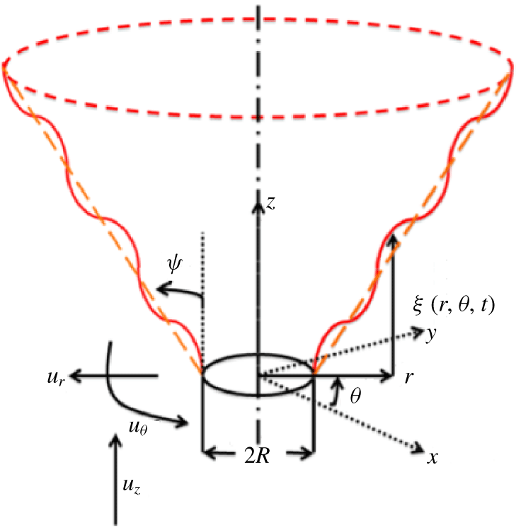
where  $\hat{u} _{ref}^{\prime }(\unicode[STIX]{x1D714},\unicode[STIX]{x1D716})$ is the reference velocity fluctuations. To motivate the importance of the nonlinear effects considered in this paper, we next discuss prior results from linear analysis. To aid in this discussion, consider the schematic in figure 3. Here, a swirling flame is stabilized on a centre body and has an inverted conical shape. The flame position is measured vertically along the axial flow direction and its instantaneous position is given by,
 $\unicode[STIX]{x1D709}(r,\unicode[STIX]{x1D703},t)$. The perturbation expansion for the flame position is expressed as
 $$\begin{eqnarray}\unicode[STIX]{x1D709}(r,\unicode[STIX]{x1D703},t)=\unicode[STIX]{x1D709}_{0}(r,\unicode[STIX]{x1D703})+\unicode[STIX]{x1D716}\unicode[STIX]{x1D709}_{1}(r,\unicode[STIX]{x1D703},t)+\unicode[STIX]{x1D716}^{2}\unicode[STIX]{x1D709}_{2}(r,\unicode[STIX]{x1D703},t)+\unicode[STIX]{x1D716}^{3}\unicode[STIX]{x1D709}_{3}(r,\unicode[STIX]{x1D703},t)+O(\unicode[STIX]{x1D716}^{4}).\end{eqnarray}$$
Schematic of the centre-body swirl-stabilized premixed flame.

The frequency domain representations for each of the fluctuations are given by
 $$\begin{eqnarray}\unicode[STIX]{x1D709}_{k}(r,\unicode[STIX]{x1D703},t)=Re\left(\mathop{\sum }_{n=1}^{\infty }\hat{\unicode[STIX]{x1D709}}_{k}(r,\unicode[STIX]{x1D703},\unicode[STIX]{x1D714}_{n})\text{e}^{\text{i}\unicode[STIX]{x1D714}_{n}t}\right).\end{eqnarray}$$
Here,  $k=1,2,3$ is the order of the flame position perturbation in the perturbation expansion shown in (1.9). Similar to (1.3)–(1.4), the flame position perturbations can be decomposed azimuthally as
 $$\begin{eqnarray}\hat{\unicode[STIX]{x1D709}}_{k}(r,\unicode[STIX]{x1D703},\unicode[STIX]{x1D714}_{n})=\mathop{\sum }_{m_{\unicode[STIX]{x1D709}k}=-\infty }^{+\infty }\hat{\unicode[STIX]{x1D701}}_{k,m_{\unicode[STIX]{x1D709}k}}(r,\unicode[STIX]{x1D714}_{n})\text{e}^{\text{i}m_{\unicode[STIX]{x1D709}k}\unicode[STIX]{x1D703}}.\end{eqnarray}$$
The azimuthal modes in the local flame disturbances,  $\unicode[STIX]{x1D709}_{k}$, of order
 $k$ are denoted by
 $m_{\unicode[STIX]{x1D709}k}$ to differentiate from the
 $j$-coordinate direction flow disturbance helical modes that are denoted by
 $m_{uj}$. The azimuthal modes in the mean flame shape are denoted by
 $m_{\unicode[STIX]{x1D709}_{0}}$. The amplitude for the flame response at mode
 $m_{\unicode[STIX]{x1D709}k}$ is denoted by
 $\hat{\unicode[STIX]{x1D701}}_{k,m_{\unicode[STIX]{x1D709}k}}$. For a nominally axisymmetric flame (i.e.
 $\unicode[STIX]{x2202}\unicode[STIX]{x1D709}_{0}/\unicode[STIX]{x2202}\unicode[STIX]{x1D703}=0$ and
 $m_{\unicode[STIX]{x1D709}_{0}}=0$ only), the
 $\text{FTF}$ takes the form (Acharya et al. Reference Acharya, Shin and Lieuwen2013)
 $$\begin{eqnarray}\text{FTF}(\unicode[STIX]{x1D714})=\mathop{\sum }_{m_{uj}}\int _{r}r\,\text{d}rg(r)\int _{\unicode[STIX]{x1D703}=0}^{\unicode[STIX]{x1D703}=2\unicode[STIX]{x03C0}}\text{e}^{\text{i}m_{uj}\unicode[STIX]{x1D703}}\,\text{d}\unicode[STIX]{x1D703}.\end{eqnarray}$$
Here,  $g(r)$ is a radial-only function depending on the mean flame,
 $\unicode[STIX]{x1D709}_{0}(r)$, and
 $\hat{\unicode[STIX]{x1D701}}_{1,m_{\unicode[STIX]{x1D709}1}}(r,\unicode[STIX]{x1D714})$ as defined in (1.11). Performing the azimuthal integration, it immediately follows that
 $\text{FTF}(\unicode[STIX]{x1D714})=0$ when
 $m_{uj}\neq 0$. In other words, helical modes exciting nominally axisymmetric flames lead to zero global unsteady heat release rate oscillations at first order in perturbation amplitude. Thus while helical modes could dominate flame wrinkling and motion, they have no influence on the linear unsteady heat release rate oscillations and only the
 $m_{uj}=0$ mode leads to spatially integrated unsteady heat release rate oscillations.
When the unperturbed nominal flame is non-axisymmetric (i.e.  $m_{\unicode[STIX]{x1D709}_{0}}\neq 0$), helical modes can excite a non-zero
 $\text{FTF}$ as discussed in prior work (Acharya & Lieuwen Reference Acharya and Lieuwen2016). In this case, the
 $\text{FTF}$ has the form
 $$\begin{eqnarray}\text{FTF}(\unicode[STIX]{x1D714})=\mathop{\sum }_{m_{\unicode[STIX]{x1D709}_{0}}}\mathop{\sum }_{m_{uj}}\int _{r}r\,\text{d}rg(r)\int _{\unicode[STIX]{x1D703}=0}^{\unicode[STIX]{x1D703}=2\unicode[STIX]{x03C0}}\text{e}^{\text{i}(m_{\unicode[STIX]{x1D709}_{0}}+m_{uj})\unicode[STIX]{x1D703}}\,\text{d}\unicode[STIX]{x1D703}.\end{eqnarray}$$
Here, the azimuthal integration is non-zero only when  $m_{\unicode[STIX]{x1D709}_{0}}+m_{uj}=0$. This indicates that asymmetric helical modes in the flow disturbances (
 $m_{uj}\neq 0$) can interact with modes in the mean flame asymmetries (
 $m_{\unicode[STIX]{x1D709}_{0}}\neq 0$) to cause a non-zero contribution to the
 $\text{FTF}$. This point demonstrates the influence of nominal flame shape on the its sensitivity to helical disturbances. Moreover, it is well known that the time-averaged flame shape changes with amplitude of excitation. Numerous studies have commented, for example, on changes in flame length with increasing excitation amplitude (Lee & Santavicca Reference Lee and Santavicca2003; Armitage et al. Reference Armitage, Balachandran, Mastorakos and Cant2006; Noiray et al. Reference Noiray, Durox, Schuller and Candel2008; Schimek et al. Reference Schimek, Moeck and Paschereit2011). This observation motivated the analysis in this paper – namely, to address the questions of whether a disturbance containing the frequency
 $\unicode[STIX]{x1D714}_{0}$ can lead to global unsteady heat release rate oscillations at
 $\unicode[STIX]{x1D714}_{0}$? Based upon the above discussion, we can hypothesize at least two mechanisms through which this can occur:
- (TA)
Azimuthal distortion of the mean flame shape by nonlinearities, leads to non-zero flame response for nominally axisymmetric flames excited by purely helical disturbances (
 $m_{uj}\neq 0$).
- (NL)
Nonlinear interactions cause purely helical velocity disturbances, (
$m_{uj}\neq 0$), to excite axisymmetric flame disturbances, ($m_{\unicode[STIX]{x1D709}k}=0$).


These will be referred to as mechanisms TA (time average) and NL (nonlinear helical mode), respectively for the rest of this paper. As will be shown later, mechanism TA is possible for a suitable superposition of single-frequency helical modes at  $O(\unicode[STIX]{x1D716}^{3})$; mechanism NL is possible for multi-frequency excitation by helical modes at
 $O(\unicode[STIX]{x1D716}^{2})$, for suitable combinations of frequency content and helical mode content. Following these points, the objective of this work is to extend the prior linear analysis to third order in perturbation amplitude to understand the nonlinear interaction of helical modes with nominally axisymmetric premixed flames. This analysis was motivated by the experimental observation (e.g. see figure 1), that the magnitude of helical modes often dominates that of axisymmetric mode in jets, particularly in swirling flows. This raises the question of whether the response of axisymmetric flames to helical flow disturbances is dominated by the linear flame sensitivity to the weaker
 $m_{uj}=0$ mode, or the nonlinear response to the higher amplitude helical modes (
 $m_{uj}\neq 0$). As noted above, nonlinearities can arise from both fluid mechanics (i.e. the nonlinear development of the shear layer disturbances) and flame dynamics. This paper focuses on the flame dynamic nonlinearity. To do this, we assume that the velocity disturbance field is imposed on the flame, and consider the nonlinear flame response. Section 2 presents the mathematical formulation for the analysis, followed by the solutions for the integrated unsteady heat release rate oscillations in § 3. Key results and discussion are included in § 4: it is possible for readers who do not wish to follow the full details of the perturbation analysis to skip directly to this section for a synopsis of the controlling physics and some illustrative examples.
2 Mathematical formulation
This section describes the basic approach used for analysing the flame response to a given disturbance. It is based on the front tracking approach for thin premixed flames (Markstein Reference Markstein1964; Matalon & Matkowsky Reference Matalon and Matkowsky1982; Williams Reference Williams1985; Boyer & Quinard Reference Boyer and Quinard1990; Fleifil et al. Reference Fleifil, Annaswamy, Ghoneim and Ghoniem1996). The flame is assumed to be located at the zero contour of an implicit function denoted as,  $G^{\ast }(r^{\ast },\unicode[STIX]{x1D703}^{\ast },z^{\ast },t^{\ast })$. The evolution of this contour is tracked using the
 $G$-equation (Markstein Reference Markstein1964; Williams Reference Williams1985).
 $$\begin{eqnarray}\frac{\unicode[STIX]{x2202}G^{\ast }}{\unicode[STIX]{x2202}t^{\ast }}+(\boldsymbol{u}^{\boldsymbol{\ast }}\boldsymbol{\cdot }\unicode[STIX]{x1D735})G^{\ast }=s_{L}^{\ast }|\unicode[STIX]{x1D735}G^{\ast }|,\end{eqnarray}$$
where  $\boldsymbol{u}^{\boldsymbol{\ast }}$ is the flow velocity vector at the flame front and the superscript ‘*’ denotes a dimensional variable. This equation is used in conjunction with the following assumptions:
(i) The flame surface is treated as a thin interface that divide the reactants and products. This assumption is valid when flame thickness/reaction length scale is much smaller than the fluid dynamic and acoustic length scales.
(ii) The location of this surface, which denotes the flame position, is a single-valued function of space (radial–azimuthal coordinate) and time. This assumption necessarily limits the amplitude of disturbances for which this analysis is valid, and the implicit
$G$-equation in (2.1) must be used directly in cases where the flame position is multi-valued.(iii) The velocity field is imposed on the flame. This implicitly assumes a weak density jump across the flame. Several researchers have analysed the alteration of the disturbance flow field due to the density change across the flame (Kuramoto & Tsuzuki Reference Kuramoto and Tsuzuki1976; Sivashinsky Reference Sivashinsky1977; Matalon & Matkowsky Reference Matalon and Matkowsky1982; Lee & Lieuwen Reference Lee and Lieuwen2003; Creta, Fogla & Matalon Reference Creta, Fogla and Matalon2011). All flames have a finite density jump; however, a weak density jump is practically applicable to combustion systems with elevated reactant preheating, which occurs in high pressure ratio systems or vitiated flows. The presence of the density change causes the Darrieus–Landau flame instability, where the approach flow is altered leading to amplification of flame wrinkles (Matalon & Matkowsky Reference Matalon and Matkowsky1982).
(iv) The propagation speed of the flame surface, denoted by
$s_{L}^{\ast }$, is assumed constant. In general, oscillatory curvature and/or hydrodynamic stretch can lead to modulation of the burning velocity. This effect becomes important at high frequencies when the convective wavelength of the disturbance is of the same order of magnitude as the Markstein length (Wang, Law & Lieuwen Reference Wang, Law and Lieuwen2009; Preetham et al. Reference Preetham, Sai, Lieuwen and Santosh2010).


Following assumption (ii), convert  $G^{\ast }(r^{\ast },\unicode[STIX]{x1D703}^{\ast },z^{\ast },t^{\ast })$ to an explicit flame position using the transformation
 $$\begin{eqnarray}G^{\ast }(r^{\ast },\unicode[STIX]{x1D703}^{\ast },z^{\ast },t^{\ast })=z^{\ast }-\unicode[STIX]{x1D709}^{\ast }(r^{\ast },\unicode[STIX]{x1D703}^{\ast },t^{\ast }).\end{eqnarray}$$
For the rest of this paper, the following non-dimensionalization scheme is used where, the velocity is normalized by  $U_{0}^{\ast }$, spatial coordinates are normalized by
 $L_{f}^{\ast }$ and time by
 $L_{f}^{\ast }/U_{0}^{\ast }$, where
 $L_{f}^{\ast }$ is the flame length. We will drop the use of the superscript ‘*’ going forward to denote the non-dimensional quantities. Using the transformation of (2.2) in (2.1), the governing equation for the flame position in polar coordinates is obtained as
 $$\begin{eqnarray}\frac{\unicode[STIX]{x2202}\unicode[STIX]{x1D709}}{\unicode[STIX]{x2202}t}+u_{r}\frac{\unicode[STIX]{x2202}\unicode[STIX]{x1D709}}{\unicode[STIX]{x2202}r}+\frac{u_{\unicode[STIX]{x1D703}}}{r}\frac{\unicode[STIX]{x2202}\unicode[STIX]{x1D709}}{\unicode[STIX]{x2202}\unicode[STIX]{x1D703}}+s_{L}\sqrt{1+\left(\frac{\unicode[STIX]{x2202}\unicode[STIX]{x1D709}}{\unicode[STIX]{x2202}r}\right)^{2}+\frac{1}{r^{2}}\left(\frac{\unicode[STIX]{x2202}\unicode[STIX]{x1D709}}{\unicode[STIX]{x2202}\unicode[STIX]{x1D703}}\right)^{2}}=u_{z}.\end{eqnarray}$$
The flame schematic is shown in figure 3. The flame base is assumed to be anchored at the centre body implying
 $$\begin{eqnarray}\unicode[STIX]{x1D709}(r=R,\unicode[STIX]{x1D703},t)=0.\end{eqnarray}$$
For the rest of this paper, we shall focus on an axisymmetric base flame (i.e.  $\unicode[STIX]{x2202}\unicode[STIX]{x1D709}_{0}/\unicode[STIX]{x2202}\unicode[STIX]{x1D703}=0$). Using (1.9) in (2.3), the evolution for the unperturbed axisymmetric base flame,
 $\unicode[STIX]{x1D709}_{0}(r)$, may then be written as
 $$\begin{eqnarray}u_{r,0}\frac{\text{d}\unicode[STIX]{x1D709}_{0}(r)}{\text{d}r}=u_{z,0}-s_{L}\sqrt{1+\left(\frac{\text{d}\unicode[STIX]{x1D709}_{0}(r)}{\text{d}r}\right)^{2}}.\end{eqnarray}$$
For convenience of notation, the following quantities are defined:
 $$\begin{eqnarray}\displaystyle & \displaystyle \frac{\text{d}\unicode[STIX]{x1D709}_{0}(r)}{\text{d}r}=\cot \unicode[STIX]{x1D713}(r), & \displaystyle\end{eqnarray}$$
 $$\begin{eqnarray}\displaystyle & \displaystyle \unicode[STIX]{x1D6E5}_{2s}=-\frac{\sin \unicode[STIX]{x1D713}(r)}{2}\left(\left(\frac{1}{r}\frac{\unicode[STIX]{x2202}\unicode[STIX]{x1D709}_{1}}{\unicode[STIX]{x2202}\unicode[STIX]{x1D703}}\right)^{2}+\sin ^{2}\unicode[STIX]{x1D713}(r)\left(\frac{\unicode[STIX]{x2202}\unicode[STIX]{x1D709}_{1}}{\unicode[STIX]{x2202}r}\right)^{2}\right), & \displaystyle\end{eqnarray}$$
 $$\begin{eqnarray}\displaystyle \unicode[STIX]{x1D6E5}_{3s} & = & \displaystyle -\frac{\sin \unicode[STIX]{x1D713}(r)}{r^{2}}\frac{\unicode[STIX]{x2202}\unicode[STIX]{x1D709}_{1}}{\unicode[STIX]{x2202}\unicode[STIX]{x1D703}}\frac{\unicode[STIX]{x2202}\unicode[STIX]{x1D709}_{2}}{\unicode[STIX]{x2202}\unicode[STIX]{x1D703}}+\frac{\cot \unicode[STIX]{x1D713}(r)\sin ^{3}\unicode[STIX]{x1D713}(r)}{2r^{2}}\frac{\unicode[STIX]{x2202}\unicode[STIX]{x1D709}_{1}}{\unicode[STIX]{x2202}r}\left(\frac{\unicode[STIX]{x2202}\unicode[STIX]{x1D709}_{1}}{\unicode[STIX]{x2202}\unicode[STIX]{x1D703}}\right)^{2}\nonumber\\ \displaystyle & & \displaystyle +\,\frac{\cot \unicode[STIX]{x1D713}(r)\sin ^{5}\unicode[STIX]{x1D713}(r)}{2}\left(\frac{\unicode[STIX]{x2202}\unicode[STIX]{x1D709}_{1}}{\unicode[STIX]{x2202}r}\right)^{3}-\cot \unicode[STIX]{x1D713}(r)\sin ^{3}\unicode[STIX]{x1D713}(r)\frac{\unicode[STIX]{x2202}\unicode[STIX]{x1D709}_{1}}{\unicode[STIX]{x2202}r}\frac{\unicode[STIX]{x2202}\unicode[STIX]{x1D709}_{2}}{\unicode[STIX]{x2202}r}.\end{eqnarray}$$
Using standard perturbation expansions, the governing equations for the flame position perturbations of different orders are given by
 $$\begin{eqnarray}\displaystyle \frac{\unicode[STIX]{x2202}\unicode[STIX]{x1D709}_{1}}{\unicode[STIX]{x2202}t}+(\boldsymbol{u}_{\boldsymbol{T},\mathbf{0}}\boldsymbol{\cdot }\unicode[STIX]{x1D735})\unicode[STIX]{x1D709}_{1}+\unicode[STIX]{x1D709}_{1}\left(\frac{\unicode[STIX]{x2202}\boldsymbol{u}_{\mathbf{0}}}{\unicode[STIX]{x2202}z}\boldsymbol{\cdot }\unicode[STIX]{x1D735}\unicode[STIX]{x1D709}_{0}\right)=u_{z,1}-(\boldsymbol{u}_{\mathbf{1}}\boldsymbol{\cdot }\unicode[STIX]{x1D735})\unicode[STIX]{x1D709}_{0}, & & \displaystyle\end{eqnarray}$$
 $$\begin{eqnarray}\displaystyle & & \displaystyle \!\!\!\frac{\unicode[STIX]{x2202}\unicode[STIX]{x1D709}_{2}}{\unicode[STIX]{x2202}t}+(\boldsymbol{u}_{\boldsymbol{T},\mathbf{0}}\boldsymbol{\cdot }\unicode[STIX]{x1D735})\unicode[STIX]{x1D709}_{2}+\unicode[STIX]{x1D709}_{2}\left(\frac{\unicode[STIX]{x2202}\boldsymbol{u}_{\mathbf{0}}}{\unicode[STIX]{x2202}z}\boldsymbol{\cdot }\unicode[STIX]{x1D735}\unicode[STIX]{x1D709}_{0}\right)\nonumber\\ \displaystyle & & \displaystyle \quad =-(\boldsymbol{u}_{\mathbf{1}}\boldsymbol{\cdot }\unicode[STIX]{x1D735})\unicode[STIX]{x1D709}_{1}-\unicode[STIX]{x1D709}_{1}\left(\frac{\unicode[STIX]{x2202}\boldsymbol{u}_{\mathbf{0}}}{\unicode[STIX]{x2202}z}\boldsymbol{\cdot }\unicode[STIX]{x1D735}\unicode[STIX]{x1D709}_{1}+\frac{\unicode[STIX]{x2202}\boldsymbol{u}_{\mathbf{1}}}{\unicode[STIX]{x2202}z}\boldsymbol{\cdot }\unicode[STIX]{x1D735}\unicode[STIX]{x1D709}_{0}\right)-\frac{\unicode[STIX]{x1D709}_{1}^{2}}{2}\left(\frac{\unicode[STIX]{x2202}^{2}\boldsymbol{u}_{\boldsymbol{ 0}}}{\unicode[STIX]{x2202}z^{2}}\boldsymbol{\cdot }\unicode[STIX]{x1D735}\unicode[STIX]{x1D709}_{0}\right)+s_{L}\unicode[STIX]{x1D6E5}_{2s},\quad \qquad\end{eqnarray}$$
 $$\begin{eqnarray}\displaystyle & & \displaystyle \frac{\unicode[STIX]{x2202}\unicode[STIX]{x1D709}_{3}}{\unicode[STIX]{x2202}t}+(\boldsymbol{u}_{\boldsymbol{T},\mathbf{0}}\boldsymbol{\cdot }\unicode[STIX]{x1D735})\unicode[STIX]{x1D709}_{3}+\unicode[STIX]{x1D709}_{3}\left(\frac{\unicode[STIX]{x2202}\boldsymbol{u}_{\mathbf{0}}}{\unicode[STIX]{x2202}z}\boldsymbol{\cdot }\unicode[STIX]{x1D735}\unicode[STIX]{x1D709}_{0}\right)\nonumber\\ \displaystyle & & \displaystyle \quad =-(\boldsymbol{u}_{\mathbf{1}}\boldsymbol{\cdot }\unicode[STIX]{x1D735})\unicode[STIX]{x1D709}_{2}-\unicode[STIX]{x1D709}_{1}\left(\frac{\unicode[STIX]{x2202}\boldsymbol{u}_{\mathbf{0}}}{\unicode[STIX]{x2202}z}\boldsymbol{\cdot }\unicode[STIX]{x1D735}\unicode[STIX]{x1D709}_{2}+\frac{\unicode[STIX]{x2202}\boldsymbol{u}_{\mathbf{1}}}{\unicode[STIX]{x2202}z}\boldsymbol{\cdot }\unicode[STIX]{x1D735}\unicode[STIX]{x1D709}_{1}\right)-\unicode[STIX]{x1D709}_{2}\left(\frac{\unicode[STIX]{x2202}\boldsymbol{u}_{\mathbf{0}}}{\unicode[STIX]{x2202}z}\boldsymbol{\cdot }\unicode[STIX]{x1D735}\unicode[STIX]{x1D709}_{1}+\frac{\unicode[STIX]{x2202}\boldsymbol{u}_{\mathbf{1}}}{\unicode[STIX]{x2202}z}\boldsymbol{\cdot }\unicode[STIX]{x1D735}\unicode[STIX]{x1D709}_{0}\right)\nonumber\\ \displaystyle & & \displaystyle \qquad -\,\frac{\unicode[STIX]{x1D709}_{1}^{2}}{2}\left(\frac{\unicode[STIX]{x2202}^{2}\boldsymbol{u}_{\boldsymbol{ 0}}}{\unicode[STIX]{x2202}z^{2}}\boldsymbol{\cdot }\unicode[STIX]{x1D735}\unicode[STIX]{x1D709}_{1}+\frac{\unicode[STIX]{x2202}^{2}\boldsymbol{u}_{\boldsymbol{ 1}}}{\unicode[STIX]{x2202}z^{2}}\boldsymbol{\cdot }\unicode[STIX]{x1D735}\unicode[STIX]{x1D709}_{0}\right)-\unicode[STIX]{x1D709}_{1}\unicode[STIX]{x1D709}_{2}\left(\frac{\unicode[STIX]{x2202}^{2}\boldsymbol{u}_{\boldsymbol{ 0}}}{\unicode[STIX]{x2202}z^{2}}\boldsymbol{\cdot }\unicode[STIX]{x1D735}\unicode[STIX]{x1D709}_{0}\right)\nonumber\\ \displaystyle & & \displaystyle \qquad +\,\frac{\unicode[STIX]{x1D709}_{1}^{3}}{6}\left(\frac{\unicode[STIX]{x2202}^{3}\boldsymbol{u}_{\boldsymbol{ 0}}}{\unicode[STIX]{x2202}z^{3}}\boldsymbol{\cdot }\unicode[STIX]{x1D735}\unicode[STIX]{x1D709}_{0}\right)+s_{L}\unicode[STIX]{x1D6E5}_{3s}.\end{eqnarray}$$
Note that the axial velocity gradients stem from spatial variations in the velocity field due to flame motion, i.e. applying a Taylor series expansion of  $\boldsymbol{u}_{\boldsymbol{j}}(r,\unicode[STIX]{x1D703},z=\unicode[STIX]{x1D709}(r,\unicode[STIX]{x1D703},t),t)$ around
 $z=\unicode[STIX]{x1D709}_{0}(r)$ using (1.9). The net tangential velocity vector,
 $\boldsymbol{u}_{\boldsymbol{T},\mathbf{0}}$, along the flame surface, due to both the azimuthal and radial velocity components, is given by
 $$\begin{eqnarray}\boldsymbol{u}_{\boldsymbol{T},\mathbf{0}}=\boldsymbol{u}_{\mathbf{0}}-s_{L}\boldsymbol{e}_{\boldsymbol{n},\mathbf{0}}.\end{eqnarray}$$
Here,  $\boldsymbol{e}_{\boldsymbol{n},\mathbf{0}}$ is the local unit normal vector, pointing from the nominal unperturbed flame surface into the products. Equations (2.9)–(2.11) show that flame wrinkles propagate along the flame surface in the direction given by
 $\boldsymbol{u}_{\boldsymbol{T},\mathbf{0}}$. The area element is given by
 $$\begin{eqnarray}\text{d}A=r\,\text{d}r\,\text{d}\unicode[STIX]{x1D703}\sqrt{1+\left(\frac{\unicode[STIX]{x2202}\unicode[STIX]{x1D709}}{\unicode[STIX]{x2202}r}\right)^{2}+\left(\frac{1}{r}\frac{\unicode[STIX]{x2202}\unicode[STIX]{x1D709}}{\unicode[STIX]{x2202}\unicode[STIX]{x1D703}}\right)^{2}}.\end{eqnarray}$$
Using the perturbation expansion for the flame position, the area element is decomposed as
 $$\begin{eqnarray}\displaystyle & \displaystyle \text{d}A_{0}=\frac{r\,\text{d}r\,\text{d}\unicode[STIX]{x1D703}}{\sin \unicode[STIX]{x1D713}(r)}, & \displaystyle\end{eqnarray}$$
 $$\begin{eqnarray}\displaystyle & \displaystyle \text{d}A_{1}=r\,\text{d}r\,\text{d}\unicode[STIX]{x1D703}\cos \unicode[STIX]{x1D713}(r)\frac{\unicode[STIX]{x2202}\unicode[STIX]{x1D709}_{1}}{\unicode[STIX]{x2202}r}, & \displaystyle\end{eqnarray}$$
 $$\begin{eqnarray}\displaystyle & \displaystyle \text{d}A_{2}=r\,\text{d}r\,\text{d}\unicode[STIX]{x1D703}\left(-\unicode[STIX]{x1D6E5}_{2s}+\cos \unicode[STIX]{x1D713}(r)\frac{\unicode[STIX]{x2202}\unicode[STIX]{x1D709}_{2}}{\unicode[STIX]{x2202}r}\right), & \displaystyle\end{eqnarray}$$
 $$\begin{eqnarray}\displaystyle & \displaystyle \text{d}A_{3}=r\,\text{d}r\,\text{d}\unicode[STIX]{x1D703}\left(-\unicode[STIX]{x1D6E5}_{3s}+\cos \unicode[STIX]{x1D713}(r)\frac{\unicode[STIX]{x2202}\unicode[STIX]{x1D709}_{3}}{\unicode[STIX]{x2202}r}\right). & \displaystyle\end{eqnarray}$$
Here,  $\unicode[STIX]{x1D6E5}_{2s}$ and
 $\unicode[STIX]{x1D6E5}_{3s}$ are defined in (2.7)–(2.8). The frequency domain component at frequency,
 $\unicode[STIX]{x1D714}$, for the area elements are denoted by
 $\text{d}\hat{A}_{k}(r,\unicode[STIX]{x1D703},\unicode[STIX]{x1D714})$, for orders
 $k=1,2,3$. The area elements can be azimuthally decomposed as
 $$\begin{eqnarray}\text{d}\hat{A}_{k}(r,\unicode[STIX]{x1D703},\unicode[STIX]{x1D714})=\mathop{\sum }_{m_{Ak}=-\infty }^{+\infty }\hat{\unicode[STIX]{x1D6FC}}_{k,Ak}(r,\unicode[STIX]{x1D714})\text{e}^{\text{i}m_{Ak}\unicode[STIX]{x1D703}}.\end{eqnarray}$$
The azimuthal mode number in the area element  $\text{d}\hat{A}_{k}(r,\unicode[STIX]{x1D703},\unicode[STIX]{x1D714})$ is
 $m_{Ak}$. Note that the global flame response in this analysis is the same as the global area response (following from the assumption of constant heat of reaction and flame speed,
 $s_{L}$). The total flame surface area is obtained by combining these expressions and integrating, and in the frequency domain is given by
 $$\begin{eqnarray}\hat{A}(\unicode[STIX]{x1D716},\unicode[STIX]{x1D714})=\int _{r}r\,\text{d}r\int _{\unicode[STIX]{x1D703}=0}^{2\unicode[STIX]{x03C0}}\left(\mathop{\sum }_{k=1}^{3}\mathop{\sum }_{m_{Ak}=-\infty }^{+\infty }\hat{\unicode[STIX]{x1D6FC}}_{k,Ak}(r,\unicode[STIX]{x1D714})\text{e}^{\text{i}m_{Ak}\unicode[STIX]{x1D703}}\right)\text{d}\unicode[STIX]{x1D703}.\end{eqnarray}$$
Note that only the area mode number  $m_{Ak}=0$ contributes to the total surface area integral. Also, the time-averaged area for the nonlinear analysis is not the same as the nominal unperturbed area. Thus, the time-average and area fluctuation corrections arise at different expansion orders as

 $$\begin{eqnarray}\displaystyle & \displaystyle A^{\prime }(\unicode[STIX]{x1D716},t)=A(\unicode[STIX]{x1D716},t)-\overline{A}(\unicode[STIX]{x1D716})=\unicode[STIX]{x1D716}A_{1}(t)+\unicode[STIX]{x1D716}^{2}(A_{2}(t)-\overline{A_{2}(t)})+\unicode[STIX]{x1D716}^{3}(A_{3}(t)-\overline{A_{3}(t)}).\quad & \displaystyle\end{eqnarray}$$
Note that for multi-frequency content in the excitation, the time average at third order is generally non-zero. The frequency domain component at frequency  $\unicode[STIX]{x1D714}$ for the area fluctuation is denoted by
 $\hat{A}^{\prime }(\unicode[STIX]{x1D716},\unicode[STIX]{x1D714})$. The flame response and flame describing function are then expressed as
 $$\begin{eqnarray}\displaystyle \left.\begin{array}{@{}c@{}}\displaystyle \hat{F}(\unicode[STIX]{x1D716},\unicode[STIX]{x1D714})=\frac{\hat{A}^{\prime }(\unicode[STIX]{x1D716},\unicode[STIX]{x1D714})}{\overline{A}(\unicode[STIX]{x1D716})},\\ \displaystyle \text{FDF}(\unicode[STIX]{x1D716},\unicode[STIX]{x1D714})=\frac{\hat{F}(\unicode[STIX]{x1D716},\unicode[STIX]{x1D714})}{\unicode[STIX]{x1D716}}.\end{array}\right\} & & \displaystyle\end{eqnarray}$$
The amplitude of the flame response,  $|\hat{F}|$ shall be used later as a measure of the global flame area dynamics. The next section shall focus on the linear and nonlinear global flame area dynamics.
3 Flame response
This section is sub-divided into three sub-sections, each of which focuses on the flame response at the first, second and third order, respectively. Given the involved nature of the mathematical details, it is useful to summarize the key mechanisms leading to nonlinear flame response. This provides a road map for seeing through the lengthy expressions to the straightforward processes that cause helical disturbances to excite non-zero unsteady heat release rate oscillations.
There are essentially two necessary criteria to have a non-zero value of  $\hat{A}^{\prime }(\unicode[STIX]{x1D716},\unicode[STIX]{x1D714}_{0})$ at the frequency
 $\unicode[STIX]{x1D714}_{0}$:
(i) First, the global area response must have a component at the frequency of interest,
$\unicode[STIX]{x1D714}_{0}$. For single-frequency excitation, $O(\unicode[STIX]{x1D716}^{2})$ effects introduce $\unicode[STIX]{x1D714}=0$ and $\unicode[STIX]{x1D714}=2\unicode[STIX]{x1D714}_{0}$ components into the global area response, where $\unicode[STIX]{x1D714}=0$ corresponds to nonlinear changes to the time-average flame shape with respect to the nominal flame shape. The $O(\unicode[STIX]{x1D716}^{3})$ effects introduce $\unicode[STIX]{x1D714}=\unicode[STIX]{x1D714}_{0}$ and $\unicode[STIX]{x1D714}=3\unicode[STIX]{x1D714}_{0}$ components. As such, the first non-zero, nonlinear response for single-frequency effects occurs at $O(\unicode[STIX]{x1D716}^{3})$. For two-frequency excitation, $\unicode[STIX]{x1D714}_{a}$ and $\unicode[STIX]{x1D714}_{b}$, nonlinear effects introduce $\unicode[STIX]{x1D714}=|\unicode[STIX]{x1D714}_{a}\pm \unicode[STIX]{x1D714}_{b}|$ frequency components at second order. As the frequency of interest for this analysis is $\unicode[STIX]{x1D714}_{0}$, if either of $|\unicode[STIX]{x1D714}_{a}\pm \unicode[STIX]{x1D714}_{b}|=\unicode[STIX]{x1D714}_{0}$, then the global area response can have a component at $O(\unicode[STIX]{x1D716}^{2})$.(ii) Second, the amplitude of the frequency component at
$\unicode[STIX]{x1D714}_{0}$ must be non-zero. As already noted, at $O(\unicode[STIX]{x1D716})$, excitation of a flame by a helical disturbance of frequency $\unicode[STIX]{x1D714}_{0}$ introduces a local response at $\unicode[STIX]{x1D714}_{0}$ everywhere on the flame, but the spatially integrated value is zero. There are two mechanisms that can cause nominally axisymmetric flames to have non-zero spatially integrated fluctuations at $\unicode[STIX]{x1D714}_{0}$. First, these disturbances can distort the time-averaged flame shape to have an azimuthal variation component that matches that of the incident disturbance, given by $\exp (\text{i}m_{uj}\unicode[STIX]{x1D703})$, referred to as ‘Mechanism TA’ in § 1. Second, multiple helical modes can nonlinearly interact to cause axisymmetric unsteady flame wrinkling, referred to as ‘Mechanism NL’.


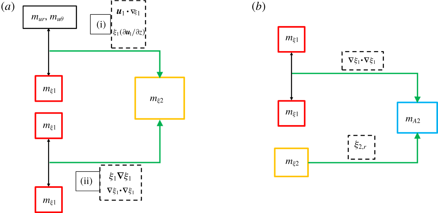
Modal interactions between source terms for the first-order contributions to local flame dynamics (left) and global flame dynamics (right). The source disturbance helical modes from the axial and radial velocity are denoted by the black boxes. These source disturbances cause (green arrow) corresponding helical disturbances in the local flame response, denoted in the red box. This leads to the corresponding first-order area response denoted by the blue box.

3.1 First-order (linear) effects
The governing dynamics for the first-order flame response was presented earlier in (2.9). The connection between modes in the source disturbances and modes in the first-order flame response are depicted in the left diagram of figure 4. The first-order area response is given by (Acharya et al. Reference Acharya, Shin and Lieuwen2013)
 $$\begin{eqnarray}\displaystyle \hat{A}_{1}(\unicode[STIX]{x1D714}_{n})=\mathop{\sum }_{m_{\unicode[STIX]{x1D709}1}=-\infty }^{+\infty }\int _{r}r\,\text{d}r\cos \unicode[STIX]{x1D713}(r)\frac{\unicode[STIX]{x2202}\hat{\unicode[STIX]{x1D701}}_{1,m_{\unicode[STIX]{x1D709}1}}(r,\unicode[STIX]{x1D714}_{n})}{\unicode[STIX]{x2202}r}\int _{\unicode[STIX]{x1D703}=0}^{2\unicode[STIX]{x03C0}}\text{e}^{\text{i}m_{uj}\unicode[STIX]{x1D703}}\,\text{d}\unicode[STIX]{x1D703}. & & \displaystyle\end{eqnarray}$$
Here,  $\hat{\unicode[STIX]{x1D701}}_{1,m_{\unicode[STIX]{x1D709}1}}$ was defined earlier in (1.11). This equation clearly shows that the azimuthal mode number in the area element is given by
 $m_{uj}$, i.e.
 $m_{A1}=m_{uj}$. This interaction is shown in the right diagram of figure 4. Here, the source helical mode is the local flame response mode denoted in the red box, which then causes (green arrow) the corresponding local flame area mode denoted in the blue box, through the term indicated in the dashed black box. From the interactions shown in figure 4, we can see that only the azimuthal mode coefficient,
 $\hat{\unicode[STIX]{x1D701}}_{1,m_{uj}=0}(r,\unicode[STIX]{x1D714}_{n})$, and thus only the axisymmetric (
 $m_{uj}=0$) flow disturbance modes, contributes to the global flame area at leading order. This was alluded to earlier in § 1, a result that has experimental support (Moeck et al. Reference Moeck, Bourgouin, Durox, Schuller and Candel2012).
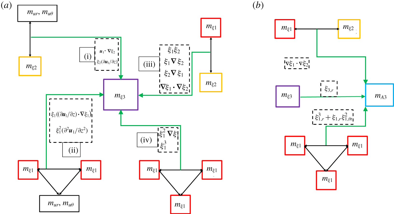
Modal interactions between source terms for the second-order contributions to local flame dynamics (a) and global flame dynamics (b). Here, the first-order flame response modes (red box) and velocity modes (black box) are the source helical modes. The interactions between the different terms are indicated by black arrows and the direction to the resultant mode is indicated by the green arrow. The second-order flame response mode, which is the focus of this figure is indicated by the orange box. The dashed black boxes indicate the interacting terms resulting in the second-order mode and have been described in the text.

3.2 Second-order effects
The second-order local flame dynamics is governed by (2.10) and is indicated by the modal interactions in figure 5(a). The second-order local flame response mode (orange box) originates through:
(i) Interactions between velocity modes (black boxes) with first-order flame response (red boxes):
(a) convective nonlinearities (terms of the form
$\boldsymbol{u}_{\mathbf{1}}\boldsymbol{\cdot }\unicode[STIX]{x1D735}\unicode[STIX]{x1D709}_{1}$), and(b) flame-motion nonlinearities (terms of the form
$(\unicode[STIX]{x2202}\boldsymbol{u}_{\mathbf{1}}/\unicode[STIX]{x2202}z)\unicode[STIX]{x1D709}_{1}$).
(ii) Self-interactions within the first-order flame response:
(a) kinematic nonlinearities (terms of the form
$\unicode[STIX]{x1D735}\unicode[STIX]{x1D709}_{1}\boldsymbol{\cdot }\unicode[STIX]{x1D735}\unicode[STIX]{x1D709}_{1}$), and(b) flame-motion nonlinearities (terms of the form
$\unicode[STIX]{x1D709}_{1}\unicode[STIX]{x1D735}\unicode[STIX]{x1D709}_{1}$).


Note that the sources of azimuthal modes in the first-order flame response (red boxes) are determined from the left diagram in figure 4. Using (2.7) and (2.16), we have
 $$\begin{eqnarray}A_{2}(t)=\int _{r}r\,\text{d}r\sin \unicode[STIX]{x1D713}(r)\int _{\unicode[STIX]{x1D703}=0}^{2\unicode[STIX]{x03C0}}\left(\frac{1}{2}\left(\left(\frac{1}{r}\frac{\unicode[STIX]{x2202}\unicode[STIX]{x1D709}_{1}}{\unicode[STIX]{x2202}\unicode[STIX]{x1D703}}\right)^{2}+\sin ^{2}\unicode[STIX]{x1D713}(r)\left(\frac{\unicode[STIX]{x2202}\unicode[STIX]{x1D709}_{1}}{\unicode[STIX]{x2202}r}\right)^{2}\right)+\cos \unicode[STIX]{x1D713}(r)\frac{\unicode[STIX]{x2202}\unicode[STIX]{x1D709}_{2}}{\unicode[STIX]{x2202}r}\right)\text{d}\unicode[STIX]{x1D703}.\end{eqnarray}$$
For discussions on nonlinear effects, the frequency contents in the flow perturbations are assumed to be integer harmonics of a fundamental frequency,  $\unicode[STIX]{x1D714}_{0}$; i.e.
 $\unicode[STIX]{x1D714}_{n}=n\unicode[STIX]{x1D714}_{0}$ where
 $n$ is a positive integer. this is done for simplicity in expressions. The qualitative arguments for all three integrals are similar, so the ensuing discussion focuses on the first integral to illustrate how these terms contribute to the second-order area fluctuations. From (1.10), we have
 $$\begin{eqnarray}\displaystyle \unicode[STIX]{x1D709}_{1,r}^{2}(r,\unicode[STIX]{x1D703},t) & = & \displaystyle \mathop{\sum }_{n_{1}=1}^{\infty }\mathop{\sum }_{n_{2}=1}^{\infty }[\!\hat{\unicode[STIX]{x1D709}}_{1,r}^{R}(n_{1}\unicode[STIX]{x1D714}_{0})\hat{\unicode[STIX]{x1D709}}_{1,r}^{R}(n_{2}\unicode[STIX]{x1D714}_{0})\cos (n_{1}\unicode[STIX]{x1D714}_{0}t)\cos (n_{2}\unicode[STIX]{x1D714}_{0}t)\nonumber\\ \displaystyle & & \displaystyle +\,\hat{\unicode[STIX]{x1D709}}_{1,r}^{R}(n_{1}\unicode[STIX]{x1D714}_{0})\hat{\unicode[STIX]{x1D709}}_{1,r}^{I}(n_{2}\unicode[STIX]{x1D714}_{0})\cos (n_{1}\unicode[STIX]{x1D714}_{0}t)\sin (n_{2}\unicode[STIX]{x1D714}_{0}t)\nonumber\\ \displaystyle & & \displaystyle +\,\hat{\unicode[STIX]{x1D709}}_{1,r}^{I}(n_{1}\unicode[STIX]{x1D714}_{0})\hat{\unicode[STIX]{x1D709}}_{1,r}^{R}(n_{2}\unicode[STIX]{x1D714}_{0})\sin (n_{1}\unicode[STIX]{x1D714}_{0}t)\cos (n_{2}\unicode[STIX]{x1D714}_{0}t)\nonumber\\ \displaystyle & & \displaystyle +\,\hat{\unicode[STIX]{x1D709}}_{1,r}^{I}(n_{1}\unicode[STIX]{x1D714}_{0})\hat{\unicode[STIX]{x1D709}}_{1,r}^{I}(n_{2}\unicode[STIX]{x1D714}_{0})\sin (n_{1}\unicode[STIX]{x1D714}_{0}t)\sin (n_{2}\unicode[STIX]{x1D714}_{0}t)\!].\end{eqnarray}$$
Here, the expressions are in the time domain and the superscripts  $R$ and
 $I$ correspond to the real and imaginary parts of the complex quantity. Although not indicated, each of
 $\hat{\unicode[STIX]{x1D709}}_{1,r}^{R,I}$ are functions of
 $(r,\unicode[STIX]{x1D703})$ also. Each of the terms can be split into two terms with frequencies:
 $|n_{1}-n_{2}|\unicode[STIX]{x1D714}_{0}$ and
 $(n_{1}+n_{2})\unicode[STIX]{x1D714}_{0}$. There are two important observations that can be made.
(a) Non-zero time-average contribution (Mechanism TA):
The terms where the frequency  $|n_{1}-n_{2}|\unicode[STIX]{x1D714}_{0}=0$ result in time-independent terms which occurs when:
 $n_{1}=n_{2}=n$. These introduce a change in the time-average flame position, corresponding to ‘Mechanism TA’. This change is expressed as
 $$\begin{eqnarray}\overline{\unicode[STIX]{x1D709}_{1,r}^{2}}=\frac{1}{2}\mathop{\sum }_{n=1}^{\infty }(\hat{\unicode[STIX]{x1D709}}_{1,r}^{R}(n\unicode[STIX]{x1D714}_{0})\hat{\unicode[STIX]{x1D709}}_{1,r}^{R}(n\unicode[STIX]{x1D714}_{0})+\hat{\unicode[STIX]{x1D709}}_{1,r}^{I}(n\unicode[STIX]{x1D714}_{0})\hat{\unicode[STIX]{x1D709}}_{1,r}^{I}(n\unicode[STIX]{x1D714}_{0})).\end{eqnarray}$$
Note that not all terms in the above summation contribute to the time average. For example, the first term can be expanded using (1.11) as
 $$\begin{eqnarray}\displaystyle \hat{\unicode[STIX]{x1D709}}_{1,r}^{R}\hat{\unicode[STIX]{x1D709}}_{1,r}^{R} & = & \displaystyle \mathop{\sum }_{m_{\unicode[STIX]{x1D709}1,1}=-\infty }^{+\infty }\mathop{\sum }_{m_{\unicode[STIX]{x1D709}1,2}=-\infty }^{+\infty }\nonumber\\ \displaystyle & & \displaystyle \times \,[\!\hat{\unicode[STIX]{x1D701}}_{1,m_{\unicode[STIX]{x1D709}1,1},r}^{R}\hat{\unicode[STIX]{x1D701}}_{1,m_{\unicode[STIX]{x1D709}1,2},r}^{R}\cos (m_{\unicode[STIX]{x1D709}1,1}\unicode[STIX]{x1D703})\cos (m_{\unicode[STIX]{x1D709}1,2}\unicode[STIX]{x1D703})\nonumber\\ \displaystyle & & \displaystyle +\,\hat{\unicode[STIX]{x1D701}}_{1,m_{\unicode[STIX]{x1D709}1,1},r}^{R}\hat{\unicode[STIX]{x1D701}}_{1,m_{\unicode[STIX]{x1D709}1,2},r}^{I}\cos (m_{\unicode[STIX]{x1D709}1,1}\unicode[STIX]{x1D703})\sin (m_{\unicode[STIX]{x1D709}1,2}\unicode[STIX]{x1D703})\nonumber\\ \displaystyle & & \displaystyle +\,\hat{\unicode[STIX]{x1D701}}_{1,m_{\unicode[STIX]{x1D709}1,1},r}^{I}\hat{\unicode[STIX]{x1D701}}_{1,m_{\unicode[STIX]{x1D709}1,2},r}^{R}\sin (m_{\unicode[STIX]{x1D709}1,1}\unicode[STIX]{x1D703})\cos (m_{\unicode[STIX]{x1D709}1,2}\unicode[STIX]{x1D703})\nonumber\\ \displaystyle & & \displaystyle +\,\hat{\unicode[STIX]{x1D701}}_{1,m_{\unicode[STIX]{x1D709}1,1},r}^{I}\hat{\unicode[STIX]{x1D701}}_{1,m_{\unicode[STIX]{x1D709}1,2},r}^{I}\sin (m_{\unicode[STIX]{x1D709}1,1}\unicode[STIX]{x1D703})\sin (m_{\unicode[STIX]{x1D709}1,2}\unicode[STIX]{x1D703})\!].\end{eqnarray}$$
Each term can be split into two terms with mode numbers ( $\pm m_{\unicode[STIX]{x1D709}1,1}\pm m_{\unicode[STIX]{x1D709}1,2}$). Thus, the azimuthal integral of these terms is non-zero only if
 $$\begin{eqnarray}\displaystyle \left.\begin{array}{@{}c@{}}m_{\unicode[STIX]{x1D709}1,1}+m_{\unicode[STIX]{x1D709}1,2}=0,\\ m_{\unicode[STIX]{x1D709}1,1}-m_{\unicode[STIX]{x1D709}1,2}=0.\end{array}\right\} & & \displaystyle\end{eqnarray}$$
Thus, the contributing terms from (3.5) can be expressed as
 $$\begin{eqnarray}\displaystyle & & \displaystyle \int _{\unicode[STIX]{x1D703}=0}^{2\unicode[STIX]{x03C0}}\hat{\unicode[STIX]{x1D709}}_{1,r}^{R}(r,\unicode[STIX]{x1D703},n\unicode[STIX]{x1D714}_{0})\hat{\unicode[STIX]{x1D709}}_{1,r}^{R}(r,\unicode[STIX]{x1D703},n\unicode[STIX]{x1D714}_{0})\,\text{d}\unicode[STIX]{x1D703}\nonumber\\ \displaystyle & & \displaystyle \quad =\unicode[STIX]{x03C0}\displaystyle \mathop{\sum }_{m_{\unicode[STIX]{x1D709}1}=-\infty }^{+\infty }[\!\hat{\unicode[STIX]{x1D701}}_{1,m_{\unicode[STIX]{x1D709}1},r}^{R}(r,n\unicode[STIX]{x1D714}_{0})\hat{\unicode[STIX]{x1D701}}_{1,m_{\unicode[STIX]{x1D709}1},r}^{R}(r,n\unicode[STIX]{x1D714}_{0})+\hat{\unicode[STIX]{x1D701}}_{1,m_{\unicode[STIX]{x1D709}1},r}^{I}(r,n\unicode[STIX]{x1D714}_{0})\hat{\unicode[STIX]{x1D701}}_{1,m_{\unicode[STIX]{x1D709}1},r}^{I}(r,n\unicode[STIX]{x1D714}_{0})\nonumber\\ \displaystyle & & \displaystyle \qquad +\,\hat{\unicode[STIX]{x1D701}}_{1,m_{\unicode[STIX]{x1D709}1},r}^{R}(r,n\unicode[STIX]{x1D714}_{0})\hat{\unicode[STIX]{x1D701}}_{1,-m_{\unicode[STIX]{x1D709}1},r}^{R}(r,n\unicode[STIX]{x1D714}_{0})-\hat{\unicode[STIX]{x1D701}}_{1,m_{\unicode[STIX]{x1D709}1},r}^{I}(r,n\unicode[STIX]{x1D714}_{0})\hat{\unicode[STIX]{x1D701}}_{1,-m_{\unicode[STIX]{x1D709}1},r}^{I}(r,n\unicode[STIX]{x1D714}_{0})\!].\end{eqnarray}$$
From the above expression, the following conclusions can be drawn:
(i) The first row of terms on the right-hand side involve the interaction of the first-order flame response at frequency
$n\unicode[STIX]{x1D714}_{0}$ and helical mode $m_{\unicode[STIX]{x1D709}1}$ with itself. Thus, there will always be a contribution to the time average, $\overline{A_{2}}$, from the second-order dynamics.(ii) The second row of terms on the right-hand side involve the interaction of the first-order flame response at frequency
$n\unicode[STIX]{x1D714}_{0}$ and helical mode $m_{\unicode[STIX]{x1D709}1}$ with the first-order flame response at the same frequency $n\unicode[STIX]{x1D714}_{0}$ and helical mode $-m_{\unicode[STIX]{x1D709}1}$. Thus, the flame responds to helical modes whose mode numbers sum to zero, and at the same frequency also contribute to the second-order correction of the time average. Note that this contribution to the time average comes from all excitation frequencies in the disturbance, regardless of the frequency of focus for $\hat{F}$ in (1.8).


In addition to the above second-order effects on the global area, the second-order correction affects the time-average flame shape as well. From (2.10), the time-averaged correction follows from the solution of
 $$\begin{eqnarray}\displaystyle & & \displaystyle \left(\frac{\unicode[STIX]{x2202}\boldsymbol{u}_{\mathbf{0}}}{\unicode[STIX]{x2202}z}\boldsymbol{\cdot }\unicode[STIX]{x1D735}\unicode[STIX]{x1D709}_{0}+(\boldsymbol{u}_{\boldsymbol{T},\mathbf{0}}\boldsymbol{\cdot }\unicode[STIX]{x1D735})\right)\overline{\unicode[STIX]{x1D709}_{2}}\nonumber\\ \displaystyle & & \displaystyle \quad =-\overline{(\boldsymbol{u}_{\mathbf{1}}\boldsymbol{\cdot }\unicode[STIX]{x1D735})\unicode[STIX]{x1D709}_{1}}-\overline{\left(\frac{\unicode[STIX]{x2202}\boldsymbol{u}_{\mathbf{0}}}{\unicode[STIX]{x2202}z}\boldsymbol{\cdot }\unicode[STIX]{x1D735}\unicode[STIX]{x1D709}_{1}+\frac{\unicode[STIX]{x2202}\boldsymbol{u}_{\mathbf{1}}}{\unicode[STIX]{x2202}z}\boldsymbol{\cdot }\unicode[STIX]{x1D735}\unicode[STIX]{x1D709}_{0}\right)\unicode[STIX]{x1D709}_{1}}-\left(\frac{\unicode[STIX]{x2202}^{2}\boldsymbol{u}_{\boldsymbol{ 0}}}{\unicode[STIX]{x2202}z^{2}}\boldsymbol{\cdot }\unicode[STIX]{x1D735}\unicode[STIX]{x1D709}_{0}\right)\overline{\frac{\unicode[STIX]{x1D709}_{1}^{2}}{2}}+s_{L}\overline{\unicode[STIX]{x1D6E5}_{2s}}.\qquad\end{eqnarray}$$
Here,  $\unicode[STIX]{x1D6E5}_{2s}$ is as in (2.7). The qualitative arguments for each of the terms are similar to the arguments used for (3.4)–(3.5) (which also happens to be one of the terms on the right-hand side of (3.8)).
Thus, the physics contributing to distortions of the time-average flame position can be summarized as:
(i) Convective nonlinearities: interaction of the first-order flame response at frequency
$n\unicode[STIX]{x1D714}_{0}$ and helical mode $m_{\unicode[STIX]{x1D709}1}$ with flow disturbances at the same frequency $n\unicode[STIX]{x1D714}_{0}$ and helical mode $m_{uj}$.(ii) Kinematic nonlinearities: interaction of the first-order flame response at frequency
$n\unicode[STIX]{x1D714}_{0}$ and helical mode $m_{\unicode[STIX]{x1D709}1,1}$ with itself at the same frequency $n\unicode[STIX]{x1D714}_{0}$ and helical mode $m_{\unicode[STIX]{x1D709}1,2}$.(iii) Flame-motion nonlinearities: flame motion causes the instantaneous imposed velocity disturbance value to differ from its value at the nominal flame position (second and third terms on the right-hand side of (3.8)).


The frequency and modal contributions can be summarized as:
(i) Frequency contributions: the contribution to the time average stems from all excitation frequencies (regardless of the frequency of focus) as they interact with themselves.
(ii) Modal contributions: in general, a non-axisymmetric correction to the time-average flame shape occurs for
(3.9)However, when$$\begin{eqnarray}m_{\unicode[STIX]{x1D709}1,1}\neq m_{\unicode[STIX]{x1D709}1,2}.\end{eqnarray}$$$m_{\unicode[STIX]{x1D709}1,1}=\pm m_{\unicode[STIX]{x1D709}1,2}=m$, the nonlinear terms are of the form $\cos ^{2}(m\unicode[STIX]{x1D703})$, $\sin ^{2}(m\unicode[STIX]{x1D703})$, $\sin (2m\unicode[STIX]{x1D703})$. In this case, the first two terms can be split into the form ($1+\cos (2m\unicode[STIX]{x1D703})$), which results in an axisymmetric and non-axisymmetric part. Thus, the nonlinear correction to the time average has a purely axisymmetric contribution whenever the axisymmetric mode interacts with itself, or from nonlinear interactions between helical modes of the same or opposite sign.




For the purposes of this analysis, those terms that distort the axisymmetric nominal flame to a time-averaged shape with an azimuthal component,  $m_{\unicode[STIX]{x1D709}_{0}}$, that matches that of the exciting helical disturbance,
 $m_{uj}$, are particularly significant, as they can lead to net flame response to helical modes; i.e. the unsteady heat release rate oscillations at third order is analogous to the linear response of a nominally non-axisymmetric flame to helical disturbances, as summarized in (1.13) in § 1.
(b) Contribution to nonlinear dynamics (Mechanism NL):
The second-order fluctuation in flame area,  $A_{2}(t)$, has a non-zero frequency component at
 $\unicode[STIX]{x1D714}_{0}$ when:
 $n_{1}\pm n_{2}=\pm 1$. The first term in (3.3) when expanded to consider only the response at
 $\unicode[STIX]{x1D714}_{0}$ is expressed as
 $$\begin{eqnarray}\displaystyle \unicode[STIX]{x1D709}_{1,r}^{2}(r,\unicode[STIX]{x1D703},t) & = & \displaystyle \frac{1}{2}\mathop{\sum }_{n=2}^{\infty }[\!\cos (\unicode[STIX]{x1D714}_{0}t)(\!\hat{\unicode[STIX]{x1D709}}_{1,r}^{R}(r,\unicode[STIX]{x1D703},n\unicode[STIX]{x1D714}_{0})\hat{\unicode[STIX]{x1D709}}_{1,r}^{R}(r,\unicode[STIX]{x1D703},(n\pm 1)\unicode[STIX]{x1D714}_{0})\nonumber\\ \displaystyle & & \displaystyle +\,\hat{\unicode[STIX]{x1D709}}_{1,r}^{I}(r,\unicode[STIX]{x1D703},n\unicode[STIX]{x1D714}_{0})\hat{\unicode[STIX]{x1D709}}_{1,r}^{I}(r,\unicode[STIX]{x1D703},(n\pm 1)\unicode[STIX]{x1D714}_{0})\!)\nonumber\\ \displaystyle & \pm & \displaystyle \sin (\unicode[STIX]{x1D714}_{0}t)(\!\hat{\unicode[STIX]{x1D709}}_{1,r}^{R}(r,\unicode[STIX]{x1D703},n\unicode[STIX]{x1D714}_{0})\hat{\unicode[STIX]{x1D709}}_{1,r}^{I}(r,\unicode[STIX]{x1D703},(n\pm 1)\unicode[STIX]{x1D714}_{0})\nonumber\\ \displaystyle & & \displaystyle -\,\hat{\unicode[STIX]{x1D709}}_{1,r}^{I}(r,\unicode[STIX]{x1D703},n\unicode[STIX]{x1D714}_{0})\hat{\unicode[STIX]{x1D709}}_{1,r}^{R}(r,\unicode[STIX]{x1D703},(n\pm 1)\unicode[STIX]{x1D714}_{0})\!)\!].\end{eqnarray}$$
Note that the interaction of the first-order flame response at the harmonic  $n\unicode[STIX]{x1D714}_{0}$ with itself at the next or prior harmonic
 $(n\pm 1)\unicode[STIX]{x1D714}_{0}$ contributes to
 $\hat{A}(\unicode[STIX]{x1D714}_{0})$. However, whether this term is non-zero is controlled by the azimuthal integral. Thus, considering the first term in the above equation as an example (and like (3.5)) and expanding
 $$\begin{eqnarray}\displaystyle & & \displaystyle \hat{\unicode[STIX]{x1D709}}_{1,r}^{R}(r,\unicode[STIX]{x1D703},n\unicode[STIX]{x1D714}_{0})\hat{\unicode[STIX]{x1D709}}_{1,r}^{R}(r,\unicode[STIX]{x1D703},n\unicode[STIX]{x1D714}_{0}\pm \unicode[STIX]{x1D714}_{0})\nonumber\\ \displaystyle & & \displaystyle \quad =\mathop{\sum }_{m_{\unicode[STIX]{x1D709}1,1}=-\infty }^{+\infty }\mathop{\sum }_{m_{\unicode[STIX]{x1D709}1,2}=-\infty }^{+\infty }[\!\hat{\unicode[STIX]{x1D701}}_{1,m_{\unicode[STIX]{x1D709}1,1},r}^{R}(r,n\unicode[STIX]{x1D714}_{0})\hat{\unicode[STIX]{x1D701}}_{1,m_{\unicode[STIX]{x1D709}1,2},r}^{R}(r,n\unicode[STIX]{x1D714}_{0}\pm \unicode[STIX]{x1D714}_{0})\cos (m_{\unicode[STIX]{x1D709}1,1}\unicode[STIX]{x1D703})\cos (m_{\unicode[STIX]{x1D709}1,2}\unicode[STIX]{x1D703})\nonumber\\ \displaystyle & & \displaystyle \qquad +\,\hat{\unicode[STIX]{x1D701}}_{1,m_{\unicode[STIX]{x1D709}1,1},r}^{R}(r,n\unicode[STIX]{x1D714}_{0})\hat{\unicode[STIX]{x1D701}}_{1,m_{\unicode[STIX]{x1D709}1,2},r}^{I}(r,n\unicode[STIX]{x1D714}_{0}\pm \unicode[STIX]{x1D714}_{0})\cos (m_{\unicode[STIX]{x1D709}1,1}\unicode[STIX]{x1D703})\sin (m_{\unicode[STIX]{x1D709}1,2}\unicode[STIX]{x1D703})\nonumber\\ \displaystyle & & \displaystyle \qquad +\,\hat{\unicode[STIX]{x1D701}}_{1,m_{\unicode[STIX]{x1D709}1,1},r}^{I}(r,n\unicode[STIX]{x1D714}_{0})\hat{\unicode[STIX]{x1D701}}_{1,m_{\unicode[STIX]{x1D709}1,2},r}^{R}(r,n\unicode[STIX]{x1D714}_{0}\pm \unicode[STIX]{x1D714}_{0})\sin (m_{\unicode[STIX]{x1D709}1,1}\unicode[STIX]{x1D703})\cos (m_{\unicode[STIX]{x1D709}1,2}\unicode[STIX]{x1D703})\nonumber\\ \displaystyle & & \displaystyle \qquad +\,\hat{\unicode[STIX]{x1D701}}_{1,m_{\unicode[STIX]{x1D709}1,1},r}^{I}(r,n\unicode[STIX]{x1D714}_{0})\hat{\unicode[STIX]{x1D701}}_{1,m_{\unicode[STIX]{x1D709}1,2},r}^{I}(r,n\unicode[STIX]{x1D714}_{0}\pm \unicode[STIX]{x1D714}_{0})\sin (m_{\unicode[STIX]{x1D709}1,1}\unicode[STIX]{x1D703})\sin (m_{\unicode[STIX]{x1D709}1,2}\unicode[STIX]{x1D703})\!].\end{eqnarray}$$
Each term can be split into two terms with mode numbers ( $m_{\unicode[STIX]{x1D709}1,1}+m_{\unicode[STIX]{x1D709}1,2}$) and (
 $m_{\unicode[STIX]{x1D709}1,1}-m_{\unicode[STIX]{x1D709}1,2}$). Thus, the azimuthal integral of these terms are non-zero only if
 $$\begin{eqnarray}m_{\unicode[STIX]{x1D709}1,1}=\pm m_{\unicode[STIX]{x1D709}1,2}.\end{eqnarray}$$
Thus, the contributing terms from (3.11) can be expressed as
 $$\begin{eqnarray}\displaystyle & & \displaystyle \int _{\unicode[STIX]{x1D703}=0}^{2\unicode[STIX]{x03C0}}\hat{\unicode[STIX]{x1D709}}_{1,r}^{R}(r,\unicode[STIX]{x1D703},n\unicode[STIX]{x1D714}_{0})\hat{\unicode[STIX]{x1D709}}_{1,r}^{R}(r,\unicode[STIX]{x1D703},n\unicode[STIX]{x1D714}_{0}\pm \unicode[STIX]{x1D714}_{0})\,\text{d}\unicode[STIX]{x1D703}\nonumber\\ \displaystyle & & \displaystyle \quad =\unicode[STIX]{x03C0}\displaystyle \mathop{\sum }_{m_{\unicode[STIX]{x1D709}1}} [\!\hat{\unicode[STIX]{x1D701}}_{1,m_{\unicode[STIX]{x1D709}1},r}^{R}(r,n\unicode[STIX]{x1D714}_{0})\hat{\unicode[STIX]{x1D701}}_{1,m_{\unicode[STIX]{x1D709}1},r}^{R}(r,n\unicode[STIX]{x1D714}_{0}\pm \unicode[STIX]{x1D714}_{0})+\hat{\unicode[STIX]{x1D701}}_{1,m_{\unicode[STIX]{x1D709}1},r}^{I}(r,n\unicode[STIX]{x1D714}_{0})\hat{\unicode[STIX]{x1D701}}_{1,m_{\unicode[STIX]{x1D709}1},r}^{I}(r,n\unicode[STIX]{x1D714}_{0}\pm \unicode[STIX]{x1D714}_{0})\nonumber\\ \displaystyle & & \displaystyle \qquad +\,\hat{\unicode[STIX]{x1D701}}_{1,m_{\unicode[STIX]{x1D709}1},r}^{R}(r,n\unicode[STIX]{x1D714}_{0})\hat{\unicode[STIX]{x1D701}}_{1,-m_{\unicode[STIX]{x1D709}1},r}^{R}(r,n\unicode[STIX]{x1D714}_{0}\pm \unicode[STIX]{x1D714}_{0})-\hat{\unicode[STIX]{x1D701}}_{1,m_{\unicode[STIX]{x1D709}1},r}^{I}(r,n\unicode[STIX]{x1D714}_{0})\hat{\unicode[STIX]{x1D701}}_{1,-m_{\unicode[STIX]{x1D709}1},r}^{I}(r,n\unicode[STIX]{x1D714}_{0}\pm \unicode[STIX]{x1D714}_{0})\!].\nonumber\\ \displaystyle & & \displaystyle\end{eqnarray}$$
Thus, the second-order contribution to the global area dynamics at frequency  $\unicode[STIX]{x1D714}_{0}$ stems from the nonlinear interaction of the first-order flame response of helical mode
 $m_{\unicode[STIX]{x1D709}1}=m$ at frequency
 $n\unicode[STIX]{x1D714}_{0}$ with the first-order flame response of helical mode
 $m_{\unicode[STIX]{x1D709}1}=\pm m$ at frequency
 $(n\pm 1)\unicode[STIX]{x1D714}_{0}$.
Finally, consider the last integration term in (3.2). Note that the symmetric mode of  $\unicode[STIX]{x1D709}_{2}$ is the only mode that contributes to the second-order flame area. The dynamics of
 $\unicode[STIX]{x1D709}_{2}$ is governed by (2.10) and, since the left-hand side operator is the same as the first-order dynamics equation, the mathematical properties of the right-hand side in the first-order case apply to the second-order dynamics as well. Thus, only an axisymmetric mode in the right-hand side terms contribute to the axisymmetric mode in the second-order local flame dynamics. Comparing (3.3) and the right-hand side of (2.10), we can see that the terms are similar in nature and thus the same arguments as for (3.5)–(3.13) apply here as well. Note that the right-hand side of (2.10) consists of terms that are due to convective nonlinearities (first term) and kinematic nonlinearities (last term:
 $\unicode[STIX]{x1D6E5}_{2s}$). Both physics contribute to the mechanism for non-zero area response through similar arguments made for the time-average contribution in the previous sub-section.
Summarizing, a non-zero second-order global flame area response at  $\unicode[STIX]{x1D714}_{0}$ occurs if:
(i) There is a flow disturbance at either
$n\unicode[STIX]{x1D714}_{0}$ and $(n+1)\unicode[STIX]{x1D714}_{0}$ (or) $n\unicode[STIX]{x1D714}_{0}$ and $(n-1)\unicode[STIX]{x1D714}_{0}$ for $n\geqslant 2$.and
(ii) The flow consists of a symmetric disturbance
$(m_{uj}=0)$ (or) at least a symmetric disturbance $(m_{uj}=0)$ and asymmetric disturbance with modes of opposite sign, i.e. both $m_{uj}=+m$ and $m_{uj}=-m$ for $m>0$.


The modal interactions for the global area dynamics are summarized in figure 5 and shall be explicitly illustrated with an example later. We next move to the discussion of the dynamics at third order.
Modal interactions between source terms for the third-order contributions to local flame dynamics (a) and global flame dynamics (b). Here, the first-order flame response modes (red box), velocity modes (black box) and second-order flame response modes (orange box) are the source helical modes. The interactions between the different terms are indicated by black arrows and the direction to the resultant mode is indicated by the green arrow. The third-order flame response mode, which is the focus of this figure, is indicated by the purple box. The third-order area response mode is shown by the blue box. The dashed black boxes indicate the interacting terms resulting in the third-order mode and have been described in the text.

3.3 Third-order effects
The third-order local flame dynamics modal interactions are determined from the right-hand side of (2.11) and shown in figure 6(a). As shown, there are several ways in which nonlinear interactions contribute at third order.
(i) Interactions between velocity modes (black box) and second-order flame response (orange box):
(a) convective nonlinearities through terms such as
$\boldsymbol{u}_{\mathbf{1}}\boldsymbol{\cdot }\unicode[STIX]{x1D735}\unicode[STIX]{x1D709}_{2}$; and(b) flame-motion nonlinearities through terms such as
$\unicode[STIX]{x1D709}_{2}(\unicode[STIX]{x2202}\boldsymbol{u}_{\mathbf{1}}/\unicode[STIX]{x2202}z)$.
(ii) Interactions between velocity modes (black box) and first-order flame response (red boxes)):
(a) flame-motion nonlinearities through terms appearing as
$\unicode[STIX]{x1D709}_{1}(\unicode[STIX]{x1D735}\unicode[STIX]{x1D709}_{1}\boldsymbol{\cdot }\unicode[STIX]{x2202}\boldsymbol{u}_{\mathbf{1}}/\unicode[STIX]{x2202}z)$ and $\unicode[STIX]{x1D709}_{1}^{2}(\unicode[STIX]{x2202}^{2}\boldsymbol{u}_{\mathbf{1}}/\unicode[STIX]{x2202}z^{2})$.
(iii) Interactions between first-order flame response (red box) and second-order flame response (orange box):
(a) kinematic nonlinearities through terms appearing as
$\unicode[STIX]{x1D735}\unicode[STIX]{x1D709}_{1}\boldsymbol{\cdot }\unicode[STIX]{x1D735}\unicode[STIX]{x1D709}_{2}$; and(b) flame-motion nonlinearities through terms appearing as
$\unicode[STIX]{x1D709}_{1}\unicode[STIX]{x1D709}_{2}$, $\unicode[STIX]{x1D709}_{1}\unicode[STIX]{x1D735}\unicode[STIX]{x1D709}_{2}$ and $\unicode[STIX]{x1D709}_{2}\unicode[STIX]{x1D735}\unicode[STIX]{x1D709}_{1}$.
(iv) Self-interactions within first-order flame modes (red boxes):
(a) flame-motion nonlinearities through terms appearing as
$\unicode[STIX]{x1D709}_{1}^{3}$ and $\unicode[STIX]{x1D709}_{1}^{2}\unicode[STIX]{x1D735}\unicode[STIX]{x1D709}_{1}$.





The modal contributions to the third-order global area dynamics (blue box) are shown in the right in figure 6. Note that the azimuthal mode number  $m_{A3}=0$ is the only contributor to the third-order global area response. To understand the modal interactions, consider the expression for the third-order global area response
 $$\begin{eqnarray}\displaystyle A_{3}(t) & = & \displaystyle \int _{r}r\,\text{d}r\int _{\unicode[STIX]{x1D703}=0}^{2\unicode[STIX]{x03C0}}\left[\frac{\sin \unicode[STIX]{x1D713}(r)}{r^{2}}\frac{\unicode[STIX]{x2202}\unicode[STIX]{x1D709}_{1}}{\unicode[STIX]{x2202}\unicode[STIX]{x1D703}}\frac{\unicode[STIX]{x2202}\unicode[STIX]{x1D709}_{2}}{\unicode[STIX]{x2202}\unicode[STIX]{x1D703}}-\frac{\cot \unicode[STIX]{x1D713}(r)\sin ^{3}\unicode[STIX]{x1D713}(r)}{2r^{2}}\frac{\unicode[STIX]{x2202}\unicode[STIX]{x1D709}_{1}}{\unicode[STIX]{x2202}r}\left(\frac{\unicode[STIX]{x2202}\unicode[STIX]{x1D709}_{1}}{\unicode[STIX]{x2202}\unicode[STIX]{x1D703}}\right)^{2}\right.\nonumber\\ \displaystyle & & \displaystyle -\left.\frac{\cot \unicode[STIX]{x1D713}(r)\sin ^{5}\unicode[STIX]{x1D713}(r)}{2}\left(\frac{\unicode[STIX]{x2202}\unicode[STIX]{x1D709}_{1}}{\unicode[STIX]{x2202}r}\right)^{3}+\cot \unicode[STIX]{x1D713}(r)\sin ^{3}\unicode[STIX]{x1D713}(r)\frac{\unicode[STIX]{x2202}\unicode[STIX]{x1D709}_{1}}{\unicode[STIX]{x2202}r}\frac{\unicode[STIX]{x2202}\unicode[STIX]{x1D709}_{2}}{\unicode[STIX]{x2202}r}+\cos \unicode[STIX]{x1D713}(r)\frac{\unicode[STIX]{x2202}\unicode[STIX]{x1D709}_{3}}{\unicode[STIX]{x2202}r}\right]\text{d}\unicode[STIX]{x1D703}.\nonumber\\ \displaystyle & & \displaystyle\end{eqnarray}$$
For illustrative purposes, consider the third term in the integrand in the above equation, as similar arguments apply to the other terms. Expanding the integrand in this term and using (3.3)
 $$\begin{eqnarray}\displaystyle & & \displaystyle \!\!\!\!2\unicode[STIX]{x1D709}_{1,r}^{3}(r,\unicode[STIX]{x1D703},t)\nonumber\\ \displaystyle & & \displaystyle \!\!\quad =\mathop{\sum }_{n_{1}=1}^{\infty }\mathop{\sum }_{n_{2}=1}^{\infty }\mathop{\sum }_{n_{3}=1}^{\infty }[\!\hat{\unicode[STIX]{x1D709}}_{1,r}^{R}(r,\unicode[STIX]{x1D703},n_{1}\unicode[STIX]{x1D714}_{0})\hat{\unicode[STIX]{x1D709}}_{1,r}^{R}(r,\unicode[STIX]{x1D703},n_{2}\unicode[STIX]{x1D714}_{0})(\cos ((n_{1}+n_{2})\unicode[STIX]{x1D714}_{0}t)+\cos ((n_{1}-n_{2})\unicode[STIX]{x1D714}_{0}t))\nonumber\\ \displaystyle & & \displaystyle \qquad +\,\hat{\unicode[STIX]{x1D709}}_{1,r}^{R}(r,\unicode[STIX]{x1D703},n_{1}\unicode[STIX]{x1D714}_{0})\hat{\unicode[STIX]{x1D709}}_{1,r}^{I}(r,\unicode[STIX]{x1D703},n_{2}\unicode[STIX]{x1D714}_{0})(\sin ((n_{1}+n_{2})\unicode[STIX]{x1D714}_{0}t)-\sin ((n_{1}-n_{2})\unicode[STIX]{x1D714}_{0}t))\nonumber\\ \displaystyle & & \displaystyle \qquad +\,\hat{\unicode[STIX]{x1D709}}_{1,r}^{I}(r,\unicode[STIX]{x1D703},n_{1}\unicode[STIX]{x1D714}_{0})\hat{\unicode[STIX]{x1D709}}_{1,r}^{R}(r,\unicode[STIX]{x1D703},n_{2}\unicode[STIX]{x1D714}_{0})(\sin ((n_{1}+n_{2})\unicode[STIX]{x1D714}_{0}t)+\sin ((n_{1}-n_{2})\unicode[STIX]{x1D714}_{0}t))\nonumber\\ \displaystyle & & \displaystyle \qquad +\,\hat{\unicode[STIX]{x1D709}}_{1,r}^{I}(r,\unicode[STIX]{x1D703},n_{1}\unicode[STIX]{x1D714}_{0})\hat{\unicode[STIX]{x1D709}}_{1,r}^{I}(r,\unicode[STIX]{x1D703},n_{2}\unicode[STIX]{x1D714}_{0})(\cos ((n_{1}+n_{2})\unicode[STIX]{x1D714}_{0}t)-\cos ((n_{1}-n_{2})\unicode[STIX]{x1D714}_{0}t))\!]\nonumber\\ \displaystyle & & \displaystyle \qquad \times \,(\hat{\unicode[STIX]{x1D709}}_{1,r}^{R}(r,\unicode[STIX]{x1D703},n_{3}\unicode[STIX]{x1D714}_{0})\cos (n_{3}\unicode[STIX]{x1D714}_{0}t)+\hat{\unicode[STIX]{x1D709}}_{1,r}^{I}(r,\unicode[STIX]{x1D703},n_{3}\unicode[STIX]{x1D714}_{0})\sin (n_{3}\unicode[STIX]{x1D714}_{0}t)).\end{eqnarray}$$
From this, we can see that the different frequencies in the time-dependent terms are ( $|\pm n_{1}\pm n_{2}\pm n_{3}|\unicode[STIX]{x1D714}_{0}$) corresponding to 4 different possibilities. Thus, any combination that corresponds to:
(i)
$|\pm n_{1}\pm n_{2}\pm n_{3}|=0$ would result in a contribution to the time average at third order, i.e. Mechanism TA.(ii)
$|\pm n_{1}\pm n_{2}\pm n_{3}|=1$ would result in a contribution to the third-order dynamics at $\unicode[STIX]{x1D714}_{0}$, i.e. Mechanism NL.



Next, we focus on the helical modes in these terms. Considering the very first term (from the product in the summation) in (3.15), we have
 $$\begin{eqnarray}\displaystyle & & \displaystyle \hat{\unicode[STIX]{x1D709}}_{1,r}^{R}(r,\unicode[STIX]{x1D703},n_{1}\unicode[STIX]{x1D714}_{0})\hat{\unicode[STIX]{x1D709}}_{1,r}^{R}(r,\unicode[STIX]{x1D703},n_{2}\unicode[STIX]{x1D714}_{0})\hat{\unicode[STIX]{x1D709}}_{1,r}^{R}(r,\unicode[STIX]{x1D703},n_{3}\unicode[STIX]{x1D714}_{0})\nonumber\\ \displaystyle & & \displaystyle \quad =\mathop{\sum }_{m_{\unicode[STIX]{x1D709}1,1}}\mathop{\sum }_{m_{\unicode[STIX]{x1D709}1,2}}\mathop{\sum }_{m_{\unicode[STIX]{x1D709}1,3}} [\!\hat{\unicode[STIX]{x1D701}}_{1,m_{\unicode[STIX]{x1D709}1,1},r}^{R}(r,n_{1}\unicode[STIX]{x1D714}_{0})\hat{\unicode[STIX]{x1D701}}_{1,m_{\unicode[STIX]{x1D709}1,2},r}^{R}(r,n_{2}\unicode[STIX]{x1D714}_{0})\cos (m_{\unicode[STIX]{x1D709}1,1}\unicode[STIX]{x1D703})\cos (m_{\unicode[STIX]{x1D709}1,2}\unicode[STIX]{x1D703})\nonumber\\ \displaystyle & & \displaystyle \qquad -\,\hat{\unicode[STIX]{x1D701}}_{1,m_{\unicode[STIX]{x1D709}1,1},r}^{R}(r,n\unicode[STIX]{x1D714}_{0})\hat{\unicode[STIX]{x1D701}}_{1,m_{\unicode[STIX]{x1D709}1,2},r}^{I}(r,n\unicode[STIX]{x1D714}_{0})\cos (m_{\unicode[STIX]{x1D709}1,1}\unicode[STIX]{x1D703})\sin (m_{\unicode[STIX]{x1D709}1,2}\unicode[STIX]{x1D703})\nonumber\\ \displaystyle & & \displaystyle \qquad -\,\hat{\unicode[STIX]{x1D701}}_{1,m_{\unicode[STIX]{x1D709}1,1},r}^{I}(r,n\unicode[STIX]{x1D714}_{0})\hat{\unicode[STIX]{x1D701}}_{1,m_{\unicode[STIX]{x1D709}1,2},r}^{R}(r,n\unicode[STIX]{x1D714}_{0})\sin (m_{\unicode[STIX]{x1D709}1,1}\unicode[STIX]{x1D703})\cos (m_{\unicode[STIX]{x1D709}1,2}\unicode[STIX]{x1D703})\nonumber\\ \displaystyle & & \displaystyle \qquad +\,\hat{\unicode[STIX]{x1D701}}_{1,m_{\unicode[STIX]{x1D709}1,1},r}^{I}(r,n\unicode[STIX]{x1D714}_{0})\hat{\unicode[STIX]{x1D701}}_{1,m_{\unicode[STIX]{x1D709}1,2},r}^{I}(r,n\unicode[STIX]{x1D714}_{0})\sin (m_{\unicode[STIX]{x1D709}1,1}\unicode[STIX]{x1D703})\sin (m_{\unicode[STIX]{x1D709}1,2}\unicode[STIX]{x1D703})\!]\nonumber\\ \displaystyle & & \displaystyle \qquad \times \, (\!\hat{\unicode[STIX]{x1D701}}_{1,m_{\unicode[STIX]{x1D709}1,3},r}^{R}(r,n_{3}\unicode[STIX]{x1D714}_{0})\cos (m_{\unicode[STIX]{x1D709}1,3}\unicode[STIX]{x1D703})-\hat{\unicode[STIX]{x1D701}}_{1,m_{\unicode[STIX]{x1D709}1,3},r}^{I}(r,n_{3}\unicode[STIX]{x1D714}_{0})\sin (m_{\unicode[STIX]{x1D709}1,3}\unicode[STIX]{x1D703})\!).\end{eqnarray}$$
Like the arguments for the frequencies, there are eight different helical modes possible, given by: ( $\pm m_{\unicode[STIX]{x1D709}1,1}\pm m_{\unicode[STIX]{x1D709}1,2}\pm m_{\unicode[STIX]{x1D709}1,3}$). Thus, for the integral to be non-zero, we must have
 $$\begin{eqnarray}\pm m_{\unicode[STIX]{x1D709}1,1}\pm m_{\unicode[STIX]{x1D709}1,2}\pm m_{\unicode[STIX]{x1D709}1,3}=0.\end{eqnarray}$$
To summarize:
(a) The third-order contribution to the time average is possible only if there are at least two excitation frequencies. This differs from the response at second order, where even a single frequency contributed to the time average. The interaction between the harmonics must be such that
$|\pm n_{1}\pm n_{2}\pm n_{3}|=0$. This is denoted by ‘Mechanism TA’ in § 1.(b) The third-order contribution to the flame dynamics at the frequency
$\unicode[STIX]{x1D714}_{0}$ is possible if there are three different harmonics such that $|\pm n_{1}\pm n_{2}\pm n_{3}|=1$ and they contain helical modes such that $\pm m_{\unicode[STIX]{x1D709}1,1}\pm m_{\unicode[STIX]{x1D709}1,2}\pm m_{\unicode[STIX]{x1D709}1,3}=0$. For the special case of a single-frequency excitation, $n_{2}=n_{3}=0$, the fundamental frequency in the source disturbances can still cause a third-order flame response when there exist different helical modes such that $\pm m_{\unicode[STIX]{x1D709}1,1}\pm m_{\unicode[STIX]{x1D709}1,2}\pm m_{\unicode[STIX]{x1D709}1,3}=0$. This is denoted by ‘Mechanism NL’ in § 1.






To further summarize, the flame response at the fundamental frequency occurs for the following:
(i) For a single-frequency case, the inter-modal interactions at second order lead to a non-axisymmetric time-average correction to the nominal flame shape. Helical modes interacting with a time-average flame shape with similar azimuthal distributions,
$m_{\unicode[STIX]{x1D709}_{0}}=\pm m_{uj}$, result in a non-zero global area response at $\unicode[STIX]{x1D714}_{0}$. Thus, the nonlinear global area response for the single-frequency case occurs at third order with the second-order dynamics contributing to changes in the time-average flame shape. Single-frequency helical modes contribute to the global area dynamics first at third order.(ii) For the multi-frequency case, second-order response consists of flame response azimuthal modes at two different frequencies interacting with each other resulting in a response at the sum and difference of the frequencies. This gives the possibility of flame response at the fundamental frequency at second order itself if the sum/difference in frequencies is equal to this fundamental frequency. If the interacting flame response azimuthal modes is of opposite sign, this results in a symmetric flame response at the fundamental frequency at second order itself, thus resulting in a second-order nonlinear global area response. Thus, for multi-frequency excitation, the global area response at the fundamental frequency happens through inter-modal, inter-frequency interactions at second order itself.


4 Example illustrations
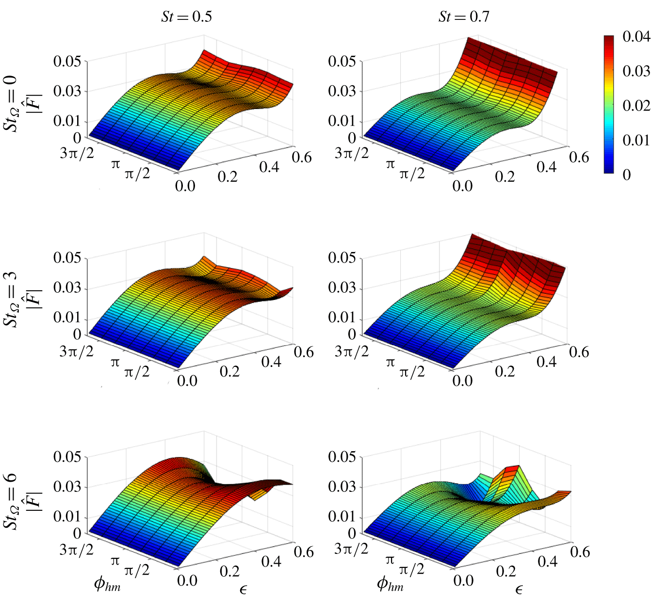
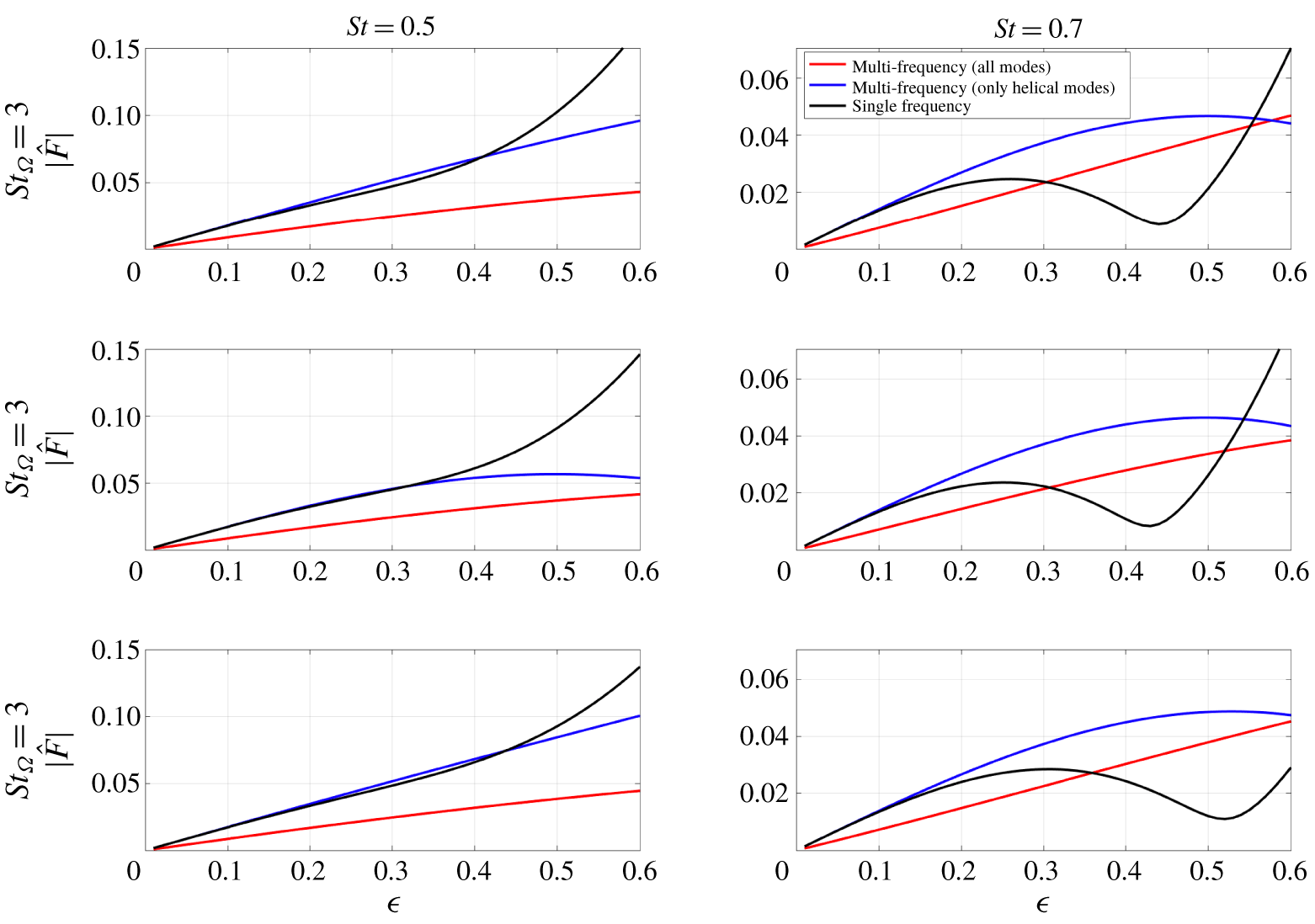
This section presents example calculations to demonstrate the points raised from the prior section explicitly. For the discussion of the examples in this section, the focus shall be on the magnitude of the flame response function  $(|\hat{F}|)$ to illustrate the effect of nonlinearity on the contribution of non-axisymmetric helical modes
 $(m_{uj}\neq 0)$ to the global area response. For the problem considered in this section, the flame response depends on several control parameters, namely helical mode numbers and their sign, relative amplitudes of the helical mode coefficients, flame angle, Strouhal number, swirling strength and disturbance convection speed. The mathematical analysis presented earlier showed that three helical modes interact under specific conditions to result in the non-zero nonlinear flame response contribution. In order to depict the different nonlinear interactions, the examples in this section are divided into focusing on:
Purely helical mode interactions (§ 4.1.1):
(i) Effects of the helical mode number values and their sign.
(ii) Effects of differences in amplitude of helical modes.
Symmetric and helical mode interactions:
(i) Effects of the amplitudes of helical modes relative to amplitude of
$m_{ur}=0$ (§ 4.1.2).(ii) Effects of relative phasing between the helical modes and the phase of the
$m_{ur}=0$ mode (§ 4.1.3).


We split the discussion into single-frequency (§ 4.1) and multi-frequency excitation (§ 4.2). In the multi-frequency excitation, we further extend results from § 4.1.2 to include a second frequency with all helical mode amplitudes being equal.
4.1 Single-frequency excitation
For the example calculations in this sub-section, the same model flow field and single-frequency excitation are used as in earlier work to facilitate comparisons (Acharya et al. Reference Acharya, Shin and Lieuwen2013)
 $$\begin{eqnarray}\left.\begin{array}{@{}c@{}}\displaystyle u_{z,0}=1\\ \displaystyle u_{r,0}=0\\ \displaystyle u_{\unicode[STIX]{x1D703},0}=\frac{\unicode[STIX]{x1D6FA}L_{f}}{u_{0}}r=St_{\unicode[STIX]{x1D6FA}}r\end{array}\right\}\;\Longrightarrow \;\left\{\begin{array}{@{}l@{}}\displaystyle \unicode[STIX]{x1D709}_{0}(r)=(r-R)\cot \unicode[STIX]{x1D713}=\tilde{r}\\ \displaystyle s_{L}=\sin \unicode[STIX]{x1D713}\end{array}\right.\end{eqnarray}$$
with the following velocity fluctuations:
 $$\begin{eqnarray}\left.\begin{array}{@{}c@{}}\displaystyle u_{r,1}=\text{Re}\left[\mathop{\sum }_{m_{uz}}\text{e}^{(-\text{i}Stt+\text{i}St_{c}z+\text{i}m_{uz}\unicode[STIX]{x1D703})}\right]\\ \displaystyle u_{z,1}=u_{\unicode[STIX]{x1D703},1}=0\end{array}\right\}\;\Longrightarrow \;\left\{\begin{array}{@{}l@{}}\displaystyle \hat{B}_{z,m_{ur}}=\text{e}^{(\text{i}St_{c}(r-R)\cot \unicode[STIX]{x1D713})}\\ \displaystyle \hat{B}_{r,m_{uz}}=\hat{B}_{\unicode[STIX]{x1D703},m_{u\unicode[STIX]{x1D703}}}=0.\end{array}\right.\end{eqnarray}$$
Here,  $u_{\unicode[STIX]{x1D703},0}=St_{\unicode[STIX]{x1D6FA}}r$, the mean swirl flow is a rigid-body rotation flow field,
 $St=\unicode[STIX]{x1D714}_{0}L_{f}/u_{0}$ is the Strouhal number denoting the non-dimensional frequency and
 $St_{c}=\unicode[STIX]{x1D714}_{0}L_{f}/u_{c}$ is the non-dimensional convective wavenumber of the helical mode.
In order to facilitate the differences in helical mode interactions, the remainder of this section is broken into different sub-sections that shall each focus on different aspects of these interactions.
4.1.1 Interactions between helical modes
Consider the amplitude-dependent response for the flow disturbances containing purely non-axisymmetric helical modes, i.e.  $m_{ur}\neq 0$. The flame response function (2.22) can be decomposed into its individual contributions as
 $$\begin{eqnarray}\hat{F}(\unicode[STIX]{x1D716},St)=\frac{\unicode[STIX]{x1D716}\hat{q}_{1}(St)+\unicode[STIX]{x1D716}^{3}\hat{q}_{3}(St)}{1+\unicode[STIX]{x1D716}^{2}\overline{q}_{2}(St)}.\end{eqnarray}$$
Here,  $\hat{q}_{1,3}=\hat{Q}_{1,3}/Q_{0}$ are the normalized flame response at first and third order and
 $\overline{q}_{2}=\overline{Q}_{2}/Q_{0}$ is the normalized second-order contribution to the time average. Since this example involves purely helical modes, we have
 $\hat{q}_{1}\equiv 0$ as discussed earlier in § 3.1. We present results here on
 $|\hat{q}_{3}|$, where the flame angle is set to
 $\unicode[STIX]{x1D713}=\unicode[STIX]{x03C0}/4$ and the non-dimensional convective wavenumber is set to
 $St_{c}=0.5$ for the remainder of the example illustrations. As the
 $O(\unicode[STIX]{x1D716}^{2})$ term in the denominator is small relative to unity,
 $|\hat{q}_{3}|$ is representative of
 $|\hat{F}|$, while also allowing us to plot results independent of
 $\unicode[STIX]{x1D716}$.
Comparison of flame response amplitude (cubic coefficient  $|\hat{q}_{3}|$) variation with swirl (
 $St_{\unicode[STIX]{x1D6FA}}$) for
 $|m_{ur}|=1,2,3$ (a) and
 $|m_{ur}|=1,3,4$ (b) for different signs of the helical modes.

First, consider two example cases with different combinations of helical modes: with  $|m_{ur}|=1,2,3$ (a),
 $|m_{ur}|=1,3,4$ (b) as shown in figure 7. Each of these cases satisfies the ‘Mechanism NL’ condition expressed earlier in (3.17). For this example, the amplitudes of all the modes are assumed to be equal, i.e.
 $\hat{B}_{r,\pm 1}=\hat{B}_{r,\pm 2}=\hat{B}_{r,\pm 3}$ and
 $\hat{B}_{r,\pm 2}=\hat{B}_{r,\pm 3}=\hat{B}_{r,\pm 5}$. The purpose of this example is to compare how the changes to the sign of the helical modes affect
 $|\hat{q}_{3}|$, and how the values of the mode numbers themselves impact the magnitude of
 $|\hat{q}_{3}|$. The figures show the variation of
 $|\hat{q}_{3}|$ with swirling strength
 $(St_{\unicode[STIX]{x1D6FA}})$ for the different helical mode combinations. Similar coloured curves correspond to the same combination of helical mode numbers but of opposite signs. In a nominally axisymmetric flame without swirl (i.e.
 $St_{\unicode[STIX]{x1D6FA}}=0$), the flame does not differentiate between sign of the velocity disturbance mode,
 $+m_{u}$ or
 $-m_{u}$, but only its magnitude,
 $|m_{u}|$. Thus, these similar coloured curves intersect when
 $St_{\unicode[STIX]{x1D6FA}}=0$. Since the nominal flame is axisymmetric,
 $St_{\unicode[STIX]{x1D6FA}}$ is a measure of the degree of symmetry breaking in the flame response. Physically, the swirling strength controls azimuthal transport of disturbances (at all orders) and thus the resulting interference of flame wrinkles. This results in the non-monotonic variation in the response amplitude as shown. Following the above point, the resulting amplitude of the flame response also depends on the sign of the helical modes for non-zero
 $St_{\unicode[STIX]{x1D6FA}}$. For example, the combination with all modes having positive sign (solid black curves), leads to the highest value of the coefficient
 $|\hat{q}_{3}|$. In addition, the value of the helical mode also has an effect. For example, the maximum amplitudes attained by the
 $|m_{ur}|=1,3,4$ cases are higher when compared to the
 $|m_{ur}|=1,2,3$ cases. This occurs because higher
 $m_{ur}$ values lead to larger azimuthal derivatives, as can be seen from the nonlinear kinematic restoration terms in (2.8).
In the above example, we used the same amplitude for all helical mode numbers. In real flows, the relative amplitudes of higher helical mode numbers is observed to be significantly lower than the lower mode numbers (see figure 1). This motivates the next example in this sub-section, which is the effect of the relative amplitudes of the different helical modes. In order to illustrate the relative amplitude effect, consider the velocity field with three modes ( $m_{1},m_{2},m_{3}$) where mode
 $m_{3}$ is the mode with a fixed amplitude and either one or both of the other modes have varying amplitudes
 $$\begin{eqnarray}\displaystyle \left.\begin{array}{@{}c@{}}\displaystyle \hat{u} _{r}(r,\unicode[STIX]{x1D703},St)=\frac{\text{e}^{(\text{i}0.5(r-R))}}{(1+2\unicode[STIX]{x1D716}_{hm})}(\unicode[STIX]{x1D716}_{hm}(\text{e}^{\text{i}m_{1}\unicode[STIX]{x1D703}}+\text{e}^{\text{i}m_{2}\unicode[STIX]{x1D703}})+\text{e}^{\text{i}m_{3}\unicode[STIX]{x1D703}}),\\ \displaystyle \hat{u} _{r}(r,\unicode[STIX]{x1D703},St)=\frac{\text{e}^{(\text{i}0.5(r-R))}}{(2+\unicode[STIX]{x1D716}_{hm})}(\unicode[STIX]{x1D716}_{hm}\text{e}^{\text{i}m_{1}\unicode[STIX]{x1D703}}+\text{e}^{\text{i}m_{2}\unicode[STIX]{x1D703}}+\text{e}^{\text{i}m_{3}\unicode[STIX]{x1D703}}),\end{array}\right\} & & \displaystyle\end{eqnarray}$$
Effect of relative amplitude  $\unicode[STIX]{x1D716}_{hm}$ on the flame response amplitude for different interacting helical modes in a (a) non-swirling and (b) swirling flow. Legend indicates combination of helical modes considered with the mode(s) whose amplitude is varied indicated within the curved braces.

Here, the relative amplitude of mode  $m_{1}$ (and/or
 $m_{2}$) with respect to the other modes is denoted by
 $\unicode[STIX]{x1D716}_{hm}$ and the scaling factor
 $(1+2\unicode[STIX]{x1D716}_{hm})$ or
 $(2+\unicode[STIX]{x1D716}_{hm})$ is to ensure that the maximum amplitude of the expression is 1 and the amplitude of the disturbance is
 $\unicode[STIX]{x1D716}$ as defined in (1.1). Figure 8 shows the variation of
 $|\hat{F}|=|\hat{q}_{3}|$ for a non-swirling (a) and a swirling case (b) for different helical mode combinations. For this example, we fix a reference mode
 $m_{3}=+1$ and consider the amplitude variations for the other modes. First consider the non-swirling case on the left. The dashed curves correspond to amplitude variations for different combinations of
 $|m_{ur}|=2,3$. For these cases, when
 $\unicode[STIX]{x1D716}_{hm}=0$, only mode
 $m_{3}=+1$ exists and thus the curves start from
 $|\hat{q}_{3}|=0$ since (3.17) is not satisfied. As
 $\unicode[STIX]{x1D716}_{hm}$ is increased, equation (3.17) is now satisfied and thus
 $|\hat{q}_{3}|$ increases to non-zero values. In contrast, for the case where the amplitude of mode
 $m_{ur}=+3$ is varied, the curve starts at a non-zero value since the remainder of the modes
 $m_{ur}=+1,+2$ satisfy (3.17). Note that, depending on the sign of the interacting modes, the quantitative variations are different indicating that the sign of the helical modes are important for the nonlinear global flame response. These differences stem from the azimuthal derivatives in the nonlinear kinematic restoration terms in (2.8). Note that, qualitatively, all curves increase to a local maximum before decreasing further, which can be attributed to changes in interference of different nonlinear terms as
 $\unicode[STIX]{x1D716}_{hm}$ is varied. A key takeaway from this example is that while
 $m_{ur}=+1$ is typically present as a mode in the unsteady flow, the introduction of the requisite higher helical modes, even at much smaller magnitudes, can lead to appreciable heat release rate oscillations through ‘Mechanism NL’. This is evident, for example, from the dashed black curve where even at
 $\unicode[STIX]{x1D716}_{hm}=0.25$, the flame response amplitude is comparable to that when all modes have equal amplitudes. In addition to the above aspects of the helical modes, swirl plays an important role in the nonlinear interactions through the bias that is introduced between positive and negative modes. Having considered purely helical mode interactions, we next consider the relative roles of the helical modes in the presence of the symmetric mode.
4.1.2 Superposition effects of $m_{ur}=0$ and helical modes $m_{ur}\neq 0$


As noted earlier, the linear response of the flame is controlled by the  $m_{ur}=0$ mode, but in many cases, helical modes have larger amplitudes. This section considers the effect of superposition of axisymmetric and non-axisymmetric velocity disturbances on the flame response. We characterize their relative strengths with the coefficient
 $\unicode[STIX]{x1D716}_{hm}$ as follows:
 $$\begin{eqnarray}u_{r,1}(r,\unicode[STIX]{x1D703},t)=\text{Re}\left[\frac{\text{e}^{(-\text{i}Stt+\text{i}St_{c}(r-R))}}{1+\unicode[STIX]{x1D716}_{hm}}\left(1+\unicode[STIX]{x1D716}_{hm}\frac{\displaystyle \mathop{\sum }_{m_{ur}\neq 0}\text{e}^{\text{i}m_{ur}\unicode[STIX]{x1D703}+\text{i}\unicode[STIX]{x1D719}_{m_{ur}}}}{\text{max}\left(\displaystyle \mathop{\sum }_{m_{ur}\neq 0}\text{e}^{\text{i}m_{ur}\unicode[STIX]{x1D703}+\text{i}\unicode[STIX]{x1D719}_{m_{ur}}}\right)}\right)\right].\end{eqnarray}$$
Here,  $\unicode[STIX]{x1D719}_{m_{ur}}$ is the phasing for helical mode
 $m_{ur}$ with respect to the axisymmetric mode
 $m_{ur}=0$. The factor
 $(1+\unicode[STIX]{x1D716}_{hm})$ is a normalization factor such that the overall maximum amplitude of this expression is 1, with the overall forcing amplitude set to
 $\unicode[STIX]{x1D716}$, as defined in the perturbation expansion in (1.1). For this example, we do not consider phase effects (
 $\unicode[STIX]{x1D719}_{m_{ur}}=0$) and we consider the helical modes,
 $m_{ur}=0,-1,+2$. This choice of the helical mode number magnitudes (i.e.
 $|m_{ur}|=1,2$) is based upon dominant modes typically observed in high Reynolds number swirl flows (see figure 1). Figure 9 shows the effect of
 $\unicode[STIX]{x1D716}_{hm}$ on the flame response for different frequencies and swirling strengths. The pure axisymmetric only case,
 $\unicode[STIX]{x1D716}_{hm}=0$, is used as a reference and is denoted by the black curves. Note the non-zero linear response for all cases. As mentioned earlier, the linear flame response depends only on the
 $m_{ur}=0$ mode (i.e. the slope from small
 $\unicode[STIX]{x1D716}$). However, note that the slopes for the different cases (red, blue, black curves) are different because of the amplitude scaling approach, see (4.5). Here, the amplitude of the
 $m_{ur}=0$ mode is scaled by
 $(1+\unicode[STIX]{x1D716}_{hm})$ and then for increasing
 $\unicode[STIX]{x1D716}_{hm}$, the slope decreases as shown. An important qualitative feature seen in the curves is that the flame response initially increases and then reaches a local maximum before decreasing to a local minimum and then continuing to monotonically increase. This non-monotonic variation has been observed in several experiments of both bluff-body and swirling flames excited by high amplitude disturbances (Thumuluru & Lieuwen Reference Thumuluru and Lieuwen2009; Bellows Reference Bellows2006; Balachandran et al. Reference Balachandran, Ayoola, Kaminski, Dowling and Mastorakos2005; Kim & Hochgreb Reference Kim and Hochgreb2011; Schimek et al. Reference Schimek, Ćosić, Moeck, Terhaar and Paschereit2015). For example, this behaviour can be seen in the data reproduced in figure 10. This behaviour occurs at this condition because of the nearly out of phase relationship between the third order,
 $\hat{q}_{3}$, and first-order flame response,
 $\hat{q}_{1}$ contributions. The
 $\hat{q}_{3}$ term is negligible relative to
 $\hat{q}_{1}$ at low
 $\unicode[STIX]{x1D716}$, but grows in importance as
 $\unicode[STIX]{x1D716}$ increases thus resulting in destructive interference effects and decreases in flame response. While the choice of helical mode magnitudes in this example (i.e.
 $|m_{ur}|=1,2$) is merely for illustration, note that such non-monotonic behaviour can occur with a range of helical mode interactions. An important takeaway from this example is that while the axisymmetric mode controls the leading-order flame response, the inclusion of the non-axisymmetric modes can significantly alter the flame response for higher amplitudes.
Relative role of asymmetric helical modes: effect of asymmetric helical mode relative amplitude  $\unicode[STIX]{x1D716}_{m}$ on the flame response amplitude.

Effect of velocity forcing amplitude on the flame response amplitude of a swirling flame. Reproduced from Thumuluru & Lieuwen (Reference Thumuluru and Lieuwen2009).

4.1.3 Effect of relative phasing between the helical modes and the symmetric mode
In the prior examples, the different helical modes were all in phase with each other. The focus of this example is to consider the effect of introducing a phasing between the different modes since this affects the destructive/constructive interference effects in the nonlinear interaction mechanisms. For this example, we use (4.5) with  $\unicode[STIX]{x1D716}_{hm}=0.5$,
 $St_{c}=0.5$ and
 $\unicode[STIX]{x1D719}_{m_{ur}}\neq 0$ to illustrate phase effects. Specifically, we consider only
 $m_{ur}=-1,+2$ and assume
 $\unicode[STIX]{x1D719}_{(m_{ur}=-1)}=0$ to consider the effects of varying
 $\unicode[STIX]{x1D719}_{(m_{ur}=+2)}=\unicode[STIX]{x1D719}_{hm}$. The variation in flame response is considered for
 $0\leqslant \unicode[STIX]{x1D719}_{hm}<2\unicode[STIX]{x03C0}$.
Effect of relative phasing  $\unicode[STIX]{x1D719}_{hm}$ between the helical modes on the nonlinear flame response amplitude.

Figure 11 shows the surface plots for the variation of the flame response amplitude with respect to forcing amplitude  $\unicode[STIX]{x1D716}$ for different values of
 $\unicode[STIX]{x1D719}_{hm}$. For the non-swirling cases
 $(St_{\unicode[STIX]{x1D6FA}}=0)$, phasing exerts minimal influence. However, for increasing swirl, the effect of phasing becomes important, due to the effect of azimuthal interference effects introduced by azimuthal convection of flame wrinkles. Note that the qualitative nature of the curves also changes with swirl and Strouhal number, as can be seen when comparing the cases for
 $St=0.7,St_{\unicode[STIX]{x1D6FA}}=3$ and
 $St=0.7,St_{\unicode[STIX]{x1D6FA}}=6$. Also, as the phasing varies, the maxima/minima seen in the curves greatly shift, indicating the overall effect of the constructive/destructive interference of flame response due to the differing phases between the helical modes. In summary, phasing has both a qualitative and quantitative effect on the flame response and is important to consider as swirling flow hydrodynamics would result in different helical modes having differing phases, often with a spatial dependence.
4.2 Multi-frequency excitation
Next, consider multi-frequency content in the disturbances to illustrate the effects of nonlinear inter-frequency interactions. Consider the case where there are two frequencies in the velocity disturbances:  $St$ and
 $2St$. We consider two forms of the velocity disturbances. First, where all modes have both frequencies
 $$\begin{eqnarray}u_{r,1}=\text{Re}\left[\frac{\text{e}^{-\text{i}Stt}+\text{e}^{-2\text{i}Stt}}{2}\left(1+\frac{\displaystyle \mathop{\sum }_{m_{ur}\neq 0}\text{e}^{\text{i}m_{ur}\unicode[STIX]{x1D703}}}{\displaystyle \text{max}\left(\mathop{\sum }_{m_{ur}\neq 0}\text{e}^{\text{i}m_{ur}\unicode[STIX]{x1D703}}\right)}\right)\right].\end{eqnarray}$$
Second, where only the asymmetric modes ( $m_{ur}\neq 0$) have both frequencies
 $$\begin{eqnarray}u_{r,1}=\text{Re}\left[\frac{\text{e}^{-\text{i}Stt}}{2}+\frac{\text{e}^{-\text{i}Stt}+\text{e}^{-2\text{i}Stt}}{4}\left(\frac{\displaystyle \mathop{\sum }_{m_{ur}\neq 0}\text{e}^{\text{i}m_{ur}\unicode[STIX]{x1D703}}}{\displaystyle \text{max}\left(\mathop{\sum }_{m_{ur}\neq 0}\text{e}^{\text{i}m_{ur}\unicode[STIX]{x1D703}}\right)}\right)\right].\end{eqnarray}$$
In both expressions, the normalization factors are such that the maximum amplitude is 1. The velocity amplitude for forcing is  $\unicode[STIX]{x1D716}$.
Effect of multi-frequency content in velocity disturbances, on the nonlinear flame response for helical mode combination  $m_{ur}=0,-1,+2$. Black: single-frequency (baseline), red: multi-frequency for all modes, blue: multi-frequency only for
 $m_{ur}=-1,+2$.

Figure 12 shows the variation in flame response amplitude ( $|\hat{F}|$) with velocity amplitude (
 $\unicode[STIX]{x1D716}$) for a radial velocity forcing with modal content
 $m_{ur}=0,-1,+2$. The baseline single-frequency case is denoted by the black curves. The plots show variations for two different frequencies:
 $St=0.5,0.7$ and three different swirling strengths:
 $St_{\unicode[STIX]{x1D6FA}}=0,3,6$. The velocity disturbances for both frequencies contain the fundamental and first harmonic, i.e.
 $St=0.5,1.0$ and
 $St=0.7,1.4$. Note that the presence of the second frequency alters the flame response noticeably. Specifically, in the case of
 $St=0.7$, the baseline case shows qualitative changes in the variation of the flame response with forcing amplitude. The local maxima and minima in the single-frequency case are absent when all the modes have multiple frequencies. Similarly, the important effect of non-uniform modal distribution across the two frequencies can be seen when comparing the blue and red curves. This is important since multiple modes and frequencies are present under large amplitude excitation conditions, as harmonics of the fundamental forcing are excited by nonlinear effects.
5 Conclusions
Swirl flows generally consist of a complex superposition of helical modes. For axisymmetric flames subjected to low amplitude disturbances, only the axisymmetric,  $m_{u}=0$ mode contributes to a global area response. However, asymmetric helical modes (
 $m_{u}\neq 0$) can lead to strong global responses at high disturbance amplitudes. Taking the thermoacoustic instability problem as a motivating example, this demonstrates that the fluid mechanic receptivity processes controlling the linear stability of the system (determined by the axisymmetric mode response to forcing) may be completely different from those controlling the finite amplitude behaviour of the system (determined also by the helical modes), e.g. large helical modes could control the flame response amplitude and thus the limit cycle.
Nonlinearities in flame response to flow disturbances arise from convection, flame kinematics and flame motion. Each of these nonlinearities contributes to the flame response in various ways. Notably, the second-order terms are seen to cause changes to the time average (with respect to the unperturbed flame) and changes to the dynamics at the fundamental frequency through interactions with neighbouring harmonics. The third-order nonlinear correction to the flame dynamics at the fundamental frequency also stems from interactions between multiple harmonics but can also stem from a single frequency interacting with itself. The non-zero contribution in each of these cases is possible only if there is a combination of helical modes (each can be at different frequencies) that sum to zero regardless of their sign. Finally, example illustrations were used to quantify the discussed effects. Notably, it was shown that the sign of the combining helical modes had an important impact on the flame response amplitude. For the cases where only purely helical modes  $(m_{ur}\neq 0)$ were interacting, the cubic coefficient in the flame response depends on both the sign and values of the combining helical modes. This coefficient increases with mode number, as they lead to larger azimuthal derivatives. Additionally, the presence of these helical modes can significantly change the qualitative nature of the flame response curve as their amplitudes become comparable to the symmetric mode amplitudes. Lastly, it was shown that the presence of a second frequency (first harmonic) in the excitation also changed both the qualitative and quantitative nature of the flame response.
These results suggest the need for a systematic set of experiments to explore these nonlinear multi-mode, multi-frequency excitation effects. In the flame response literature, there are a number of studies that have systematically analysed the amplitude dependence of the flame response, as a function of axisymmetric forcing amplitude (e.g. see figure 10). While helical modes may be present under these conditions, they have not been as carefully characterized. These results show the need for experiments where modal triads are systematically excited, their relative amplitudes characterized, and the resulting flame response quantified. Such multi-modal excitation has been performed for non-reacting shear flow problems (Cohen & Wygnanski Reference Cohen and Wygnanski1987a,Reference Cohen and Wygnanskib; Reynolds et al. Reference Reynolds, Parekh, Juvet and Lee2003), with limited research on corresponding flame response to multi-frequency excitation (Balachandran, Dowling & Mastorakos Reference Balachandran, Dowling and Mastorakos2008).
Acknowledgements
This research was partially supported by the Air Force Office of Scientific Research (FA9550-16-1-0442 monitored by Dr C. Li) and the Department of Energy (UTSR program contract DE-FE0031285 monitored by M. Freeman). The clusters offered through the NSF XSEDE program under charge number TG-CTS1600187 were used for the numerical simulations in the time domain.
Declaration of interests
The authors report no conflict of interest.