

1. INTRODUCTION
The field of non-linear effects in plasmas has grown rapidly during last few decades due to the availability of high-power laser beams. In the wide spectrum of non-linear effects, self-focusing/defocusing of laser beams (Akhmanov et al., Reference Akhmanov, Sukhorukov and Khokhlov1968) occupies significant place in the field of laser–plasma interaction due to its relevance to laser-based plasma accelerators (Malka, Reference Malka2012; Hooker, Reference Hooker2013), laser-driven fusion (Atzeni, Reference Atzeni2015; Betti & Hurricane, Reference Betti and Hurricane2016), harmonic generation (Kaur et al., Reference Kaur, Sharma and Salih2009; Zhang & Thomas, Reference Zhang and Thomas2015; Vij et al., Reference Vij, Kant and Aggarwal2016), ion acceleration (Tripathi et al., Reference Tripathi, Taguchi and Liu2005), new radiation sources (Brenner et al., Reference Brenner, Mirfayzi, Rusby, Armstrong, Alejo, Wilson, Clarke, Ahmed, Butler, Haddock, Higginson, McCLYMONT, Murphy, Notley, Oliver, Allott, Hernadez-Gomez, Kar, McKENNA and Neely2016; Ferri et al., Reference Ferri, Davoine, Kalmykov and Lifschitz2016), ionospheric modification (Keskinen & Basu, Reference Keskinen and Basu2003; Gondarenko et al., Reference Gondarenko, Ossakow and Milikh2005), etc. In plasmas, the self-focusing of laser beams, having a non-uniform distribution of irradiance along the wavefront is caused by the corresponding non-uniform distribution of the dielectric function of the plasma media on account of inherent non-linearities (Sodha et al., Reference Sodha, Sharma and Agarwal2006). Three types of non-linearities, viz., relativistic, ponderomotive, and collisional have been identified. The role of these non-linearities in the self-focusing of the beams has received considerable attention in the last 50 years. The phenomenon of self-focusing associated with the interaction of intense laser beams with plasmas occurs due to the laser-induced changes in the dielectric properties of plasma. Since the non-linear effects in plasmas are highly sensitive to the intensity distribution along the wavefront of the beam, which is significantly affected by self-focusing, the magnitude of all non-linear processes in plasmas is affected by this phenomenon. In case of collisionless plasma, the ponderomotive force on the electrons is proportional to the gradient of the irradiance, which causes a redistribution of the electron density and thereby the dielectric function. Such non-linearity sets in a period of the order r 0/c s, where r 0 is the width of the beam and c s is the ion sound speed. Hence, for collisionless plasma at moderate fields of the laser beam, there is a modification of electron density and subsequent alteration in the dielectric function of the plasma causing self-focusing/defocusing of the beam (Sodha et al., Reference Sodha, Ghatak and Tripathi1976).
The theoretical analysis based on a paraxial approach for self-focusing of laser beams in non-linear medium (Akhmanov et al., Reference Akhmanov, Sukhorukov and Khokhlov1968) has been extended by Sodha et al. (Reference Sodha, Ghatak and Tripathi1976) for plasmas. Most of the research work (Jha et al., Reference Jha, Mishra, Upadhyay and Raj2006; Asthana et al., Reference Asthana, Rathore and Varshney2009, Reference Asthana, Rathore and Varshney2012; Xiong et al., Reference Xiong, Liu, Liao and Liu2010; Malekshahi et al., Reference Malekshahi, Dorranian and Askari2014; Aggarwal et al., Reference Aggarwal, Kumar and Kant2016; Kumar et al., Reference Kumar, Aggarwal and Gill2016; Wani & Kant, Reference Wani and Kant2017) on self-focusing of laser beams in magnetized plasma has been confined to cylindrically symmetric Gaussian beam. Upadhyay et al. (Reference Upadhyay, Tripathi, Sharma and Pant2002) have studied the asymmetric self-focusing of the laser pulse in plasma and highlighted that over a distance of a few Rayleigh lengths, the temporal profile of the laser acquires significant asymmetry. Survey of literature has shown that there are many beams with a variety of intensity profiles. The beam shaping technology has made these beams available practically. Only few investigations have been reported on self-focusing of elliptic Gaussian beams (Soni & Nayyar, Reference Soni and Nayyar1980; Singh et al., Reference Singh, Aggarwal and Gill2008), Laguerre-Gaussian beams (Khamedi & Bahrampour, Reference Khamedi and Bahrampour2013), hollow Gaussian beams (Hussain et al., Reference Hussain, Singh, Singh and Sharma2014), super-Gaussian beams (Gill et al., Reference Gill, Kaur and Mahajan2015), Hermite-Gaussian beams (Takale et al., Reference Takale, Navare, Patil, Fulari and Dongare2009; Kant et al., Reference Kant, Wani and Kumar2012), quadruple Gaussian beams (Aggarwal et al., Reference Aggarwal, Vij and Kant2015a , Reference Aggarwal, Vij and Kant b ), etc. The non-linear effects arrived by these laser beams in plasmas are highly sensitive to the distribution of intensity along the wavefronts of the laser beams and laser–plasma coupling parameters. A new class of laser beams known as cosh-Gaussian beams (Lu et al., Reference Lu, Ma and Zhang1999) has received significant interest as these beams possess high power and low divergence in comparison to the Gaussian beam (Konar et al., Reference Konar, Mishra and Jana2007). Such beams thus can be utilized to achieve efficient interaction with the plasmas without being absorbed. The investigations on interaction of cosh-Gaussian beams with plasmas (Gill et al., Reference Gill, Mahajan and Kaur2011; Patil et al. Reference Patil, Takale, Navare and Dongare2011, Reference Patil, Takale, Navare, Fulari and Dongare2012; Patil & Takale, Reference Patil and Takale2013; Aggarwal et al., Reference Aggarwal, Vij and Kant2014; Nanda & Kant, Reference Nanda and Kant2014; Kant & Wani, Reference Kant and Wani2015), till date, to the best of author's knowledge, are limited to their intensity profile with circular symmetric cross-sectional area. Since many laser systems produce a beam that is more nearly elliptical and the ellipticity of the beams leads to deviation from circular symmetry, it is worthwhile to undertake such realistic situation. Moreover, self-focusing of symmetric Hermite-cosh-Gaussian laser beams (Patil et al., Reference Patil, Takale, Navare, Fulari and Dongare2007, Reference Patil, Takale, Navare and Dongare2010; Kaur et al., Reference Kaur, Kaur, Kaur and Gill2017) in plasmas has received considerable attention in different situations.
The aim of this paper is to investigate self-focusing of asymmetric cosh-Gaussian laser beams in collisionless magnetized plasma. We have done theoretical study concerned with beam-width parameter changes, which are related to the transverse dimensions of the beam during the propagation through the plasma. The present study employs WKB and paraxial approximations under usual parabolic equation approach (Akhmanov et al., Reference Akhmanov, Sukhorukov and Khokhlov1968). The systematic organization of the paper is as follows: In the Propagation dynamics section, we have given intensity profile of the cosh-Gaussian beam, a non-linear dielectric function for collisionless magnetized plasma and setup the coupled differential equations of beam-width parameters in both transverse dimensions of the beam. In the Results and discussion section, a detailed discussion of the results has been presented. A brief conclusion is finally added in the Conclusion section.
2. PROPAGATION DYNAMICS
In the slowly varying envelope approximation, the evolution of the electric field (for right circularly polarized also called extraordinary mode) in collisionless magnetized plasma can be written as (Sodha et al., Reference Sodha, Ghatak and Tripathi1976)
 $$\eqalign{& \displaystyle{{\partial ^2E_ +} \over {\partial z^2}} - 2ik_ + \displaystyle{{\partial E_ +} \over {\partial z}} + {\rm \delta} _ + \left( {\displaystyle{{\partial ^2} \over {\partial x^2}} + \displaystyle{{\partial ^2} \over {\partial y^2}}} \right)E_ + \cr & + \displaystyle{{{\rm \omega} ^2} \over {c^2}}({\rm \varepsilon} _ + - {\rm \varepsilon} _{0 +} )E_ + = 0,} $$
where δ+ = [1 + (ε0+/ε0zz
)]/2 with
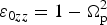 ${\rm \varepsilon} _{0zz} = 1 - \Omega _{\rm p}^2 $
. The effective dielectric function ε+ of the plasma can be expressed in the form given by
 $${\rm \varepsilon} _ + = {\rm \varepsilon} _{0 +} + {\rm \phi} _ + (E_ + E_ + ^* ),$$
where ε0+ and ϕ+ represents the linear and non-linear parts of ε+, respectively with
 $${\rm \varepsilon} _{0 +} = 1 - \displaystyle{{\Omega _{\rm p}^2} \over {(1 - \Omega _{\rm c})}},$$
 $${\rm \phi} _ + = \displaystyle{{\Omega _{\rm p}^2} \over {2(1 - \Omega _{\rm c}^2 )}}[1 - \exp \{ - ({\rm \gamma} _ + {\rm \alpha} E_{0 +} ^2 )\} ],$$
where γ+ = [1 − (Ωc/2)]/(1 − Ωc), α = 3mα0/4M, α0 = e 2/6mω2 K B T 0, Ωp = ωp/ω, ωp = (4πN 0 e 2/m)1/2 is the plasma frequency, Ωc = ωc/ω, ωc = eB 0/mc is the electron cyclotron frequency.
Here, e and m are the electronic charge and its rest mass respectively, N 0 is the unperturbed density of plasma electrons, M is the mass of ion, ω is the angular frequency of laser used, K B is the Boltzmann constant, B 0 is the static magnetic field, and T 0 is the equilibrium plasma temperature.
Introducing the concept of eikonal, one can express E + as
 $$E_ + = A_{0 +} \,(x,y,z)\exp [ - ik_ + S_ + (x,y,z)],$$
where S + is the eikonal of the beam and is related to the curvature of the wavefront of the beam.
Within the framework of WKB and paraxial approximations, for initially cosh-Gaussian beams, one finds
 $$A_{0 +} ^2 = \displaystyle{{E_{0 +} ^2} \over {\,f_{1 +} f_{2 +}}} \left[ \matrix{\exp \left( \displaystyle{{b_1^2} \over 4} \right)\left\{ \exp \left[ - \left( \displaystyle{x \over {r_{0 +} f_{1 +}}} + \displaystyle{{b_1} \over 2} \right)^2 \right]\right. \cr \left. \;\;+ \exp \left[ - \left( \displaystyle{x \over {r_{0 +} f_{1 +}}} - \displaystyle{{b_1} \over 2} \right)^2 \right] \right\} \hfill \cr \exp \left( \displaystyle{{b_2^2} \over 4} \right)\left\{ \exp \left[ - \left( \displaystyle{y \over {r_{0 +} f_{2 +}}} + \displaystyle{{b_2} \over 2} \right)^2 \right] \right. \cr \left.{\hskip-19pt}+ \exp \left[ - \left( \displaystyle{y \over {r_{0 +} f_{2 +}}} - \displaystyle{{b_2} \over 2} \right)^2 \right] \right\}} \right]^2,$$
and
 $$S_ + = \displaystyle{1 \over {{\rm \delta} _ +}} \left( {\displaystyle{{x^2} \over {2f_{1 +}}} \displaystyle{{df_{1 +}} \over {dz}} + \displaystyle{{y^2} \over {2f_{2 +}}} \displaystyle{{df_{2 +}} \over {dz}}} \right) + {\rm \psi} _ + (z),$$
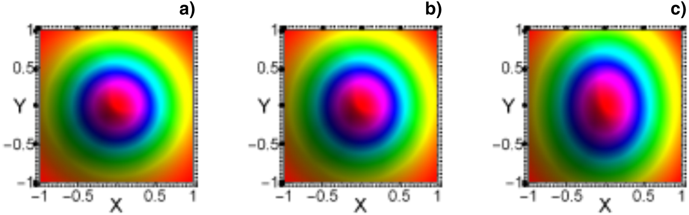
where E 0+ is the initial amplitude of the Gaussian laser beam with initial beam-width r 0+; b 1 and b 2 are the decentered parameters of cosh-Gaussian beams with f 1+ and f 2+ as the corresponding beam-width parameters in x and y dimensions, respectively. Such decentered laser beams can be produced in the laboratory by reflection of Gaussian laser beams from a spherical mirror whose center is offset from a beam axis (Al-Rashed & Saleh, Reference Al-Rashed and Saleh1995). The cosh-Gaussian laser beams can thus be produced by the superposition of two such decentered laser beams that are having same spot size and are in phase with each other. Figure 1 depicts the initial beam profiles (above orthographic view) for different decentered parameters in transverse dimensions of the beam. From this figure, it is clear that for intensity profile with symmetric decentered parameters (b 1 = b 2 = 0.0), beam recovers circularly symmetric view (Gaussian) as shown in Figure 1(a). Figure 1(b) portrays the corresponding view for asymmetric decentered parameters (b 1 = 0.2, b 2 = 0.6) in transverse dimensions of the beam. It shows a slight deviation from circular symmetry in case of the cosh-Gaussian profile. It is obvious that due to the unlike decentering (b 2 >b 1), such deviation is more in y than x dimensions of the beam. For decentered parameters b 1 = 0.4, b 2 = 0.8, the corresponding view has been presented in Figure 1(c). It is to be noted from Figure 1 that two unlike decentered parameters in transverse dimensions of the beam justify the ellipticity in case of cosh-Gaussian intensity profile.
The above orthographic view of initial 3D intensity profiles of cosh-Gaussian laser beams; (a) b 1 = b 2 = 0.0; (b) b 1 = 0.2, b 2 = 0.6; and (c) b 1 = 0.4, b 2 = 0.8.
Following the approach given by Akhmanov et al. (Reference Akhmanov, Sukhorukov and Khokhlov1968) and its extension by Sodha et al. (Reference Sodha, Ghatak and Tripathi1976), we have obtained expressions for beam-width parameters f 1+ and f 2+ as
 $$\displaystyle{{d^2f_{1 +}} \over {d{\rm \zeta} _ + ^2}} = \displaystyle{{A_1} \over 2}\displaystyle{{{\rm \delta} _ + ^2} \over {\,f_{1 +} ^3}} + \displaystyle{{B_1{\rm \delta} _ +} \over {(1 - \Omega _{\rm c})}}\displaystyle{{{\rm \rho} _{0 +}^2 \Omega^2_{\rm p} {\rm \gamma} _ + p_{0 +}} \over {\,f_{1 +} ^3 f_{2 +} ^2}} \exp \left( { - \displaystyle{{{\rm \gamma} _ + p_{0 +}} \over {\,f_{1 +} f_{2 +}}}} \right),$$
 $$\displaystyle{{d^2f_{2 +}} \over {d{\rm \zeta} _ + ^2}} = \displaystyle{{A_2} \over 2}\displaystyle{{{\rm \delta} _ + ^2} \over {\,f_{2 +} ^3}} + \displaystyle{{B_2{\rm \delta} _ +} \over {(1 - \Omega _{\rm c})}}\displaystyle{{{\rm \rho} _{0 +}^2 {\rm \Omega} _{\rm p}^2 {\rm \gamma} _ + p_{0 +}} \over {\,f_{2 +} ^3 f_{1 +} ^2}} \exp \left( { - \displaystyle{{{\rm \gamma} _ + p_{0 +}} \over {\,f_{2 +} f_{1 +}}}} \right),$$
where
 $A_{1,2} = 4(1 - b_{1,2}^2 )$
,
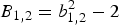 $B_{1,2} = b_{1,2}^2 - 2$
,
 $p_{0 +} = {\rm \alpha} E_{0 +} ^2 $
; ρ0+ = r
0+ω/c is the equilibrium beam radius;
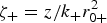 ${\rm \zeta} _ + = {z / {k_ + r_{0 +} ^2}} $
is the dimensionless distance of propagation.
For an initially plane wavefront, df
1+,2+/dζ+ = 0 and f
1+,2+ = 1 at ζ+ = 0, the conditions
 ${{d^2f_{1 +, 2 +}} / {d{\rm \zeta} _ + ^2 = 0}}$
lead to the propagation of cosh-Gaussian laser beams without convergence or divergence, i.e. in self-trapped mode. These conditions are known as critical conditions. Thus, by putting
 ${{d^2f_{1 +, 2 +}} / {d{\rm \zeta} _ + ^2 = 0}}$
in Eqs. (7) and (8), we obtain relations between ρ01+ and ρ02+ in both x and y dimensions as
 $${\rm \rho} _{01 +} ^2 = - \displaystyle{{A_1{\rm \delta} _ + (1 - \Omega _{\rm c})} \over {2B_1\Omega _{\rm p}^2 \;{\rm \gamma} _ + p_{0 +}}} \;\exp ({\rm \gamma} _ + p_{0 +} ),$$
 $${\rm \rho} _{02 +} ^2 = - \displaystyle{{A_2\delta _ + (1 - \Omega _{\rm c})} \over {2B_2\Omega _{\rm p}^2 \;{\rm \gamma} _ + p_{0 +}}} \exp ( {\rm \gamma} _ + p_{0 +} ).$$
As the formulation for both the extraordinary and ordinary (E-mode and O-mode) is similar, we can develop the corresponding expressions for ordinary mode by replacing ωc with −ωc.
3. RESULTS AND DISCUSSION
Equations (7) and (8) are second-order, coupled, non-linear differential equations governing self-focusing/defocusing of asymmetric cosh-Gaussian laser beams in collisionless magnetized plasma. First term on the right-hand sides of Eqs. (7) and (8) represents diffractional term, which leads to divergence of the beam, while the second term is the non-linear term, which is responsible for the convergence or self-focusing of the beam. Obviously, the self-focusing or defocusing of the beam for a given initial beam-width is determined by the relative magnitude of diffractional and non-linear terms of Eqs. (7) and (8). We have solved these equations simultaneously by using fourth-order Runge-Kutta method by applying the initial conditions at ζ± = 0, f 1±,2± = 1 and df 1±,2±/dζ± = 0. The requisite laser–plasma parameters are: ω = 1.778 × 10¹⁴ rad/s, N 0 = 1019 cm−3, B 0 = 0.10 − 0.20 MG, b 1,2 = 0.0 − 0.8, ρ01+,02+ = 4, and p 0+ = 0.5.
Figure 2 illustrates the critical curves for E-mode in collisionless magnetized plasma. It is noticed from this figure that the value of equilibrium beam radius ρ0+ with initial intensity parameter p 0+ decreases initially and slowly attains a constant value. As obvious, the value of ρ0+ is further affected by the density of plasma electrons, the strength of the external magnetic field, and decentered parameters b 1,2, etc. The region above the respective curves corresponds to the focused region and below, the defocused region. Figure 2 shows that if the decentered parameters in both the dimensions are equal, then corresponding curves for ρ01+ and ρ02+ merge together. This indicates that the beam is circularly symmetric for identical b values along both the dimensions of the beam. Further, if b values are different in x and y dimensions, the corresponding curves are not identical due to the asymmetry in the beam profile. The focusing region increases with increase in decentered parameters in both the dimensions.
Critical curves for E-mode in collisionless magnetized plasma. Solid curve corresponds to decentered parameters, b 1 = b 2 = 0.0, dashed curve corresponds to b 1 = 0.2 and b 2 = 0.6, dotted curve corresponds to b 1 = 0.4 and b 2 = 0.8. Thick curves are for ρ01+ and thin curves are for ρ02+. The other parameters are ω = 1.778 × 10¹⁴ rad/s, N 0 = 1019 cm−3, B 0 = 0.10 MG.
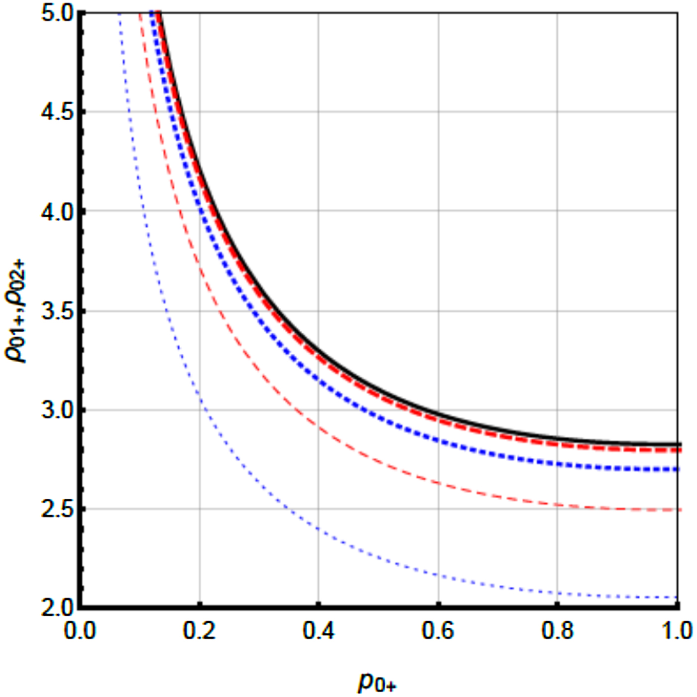
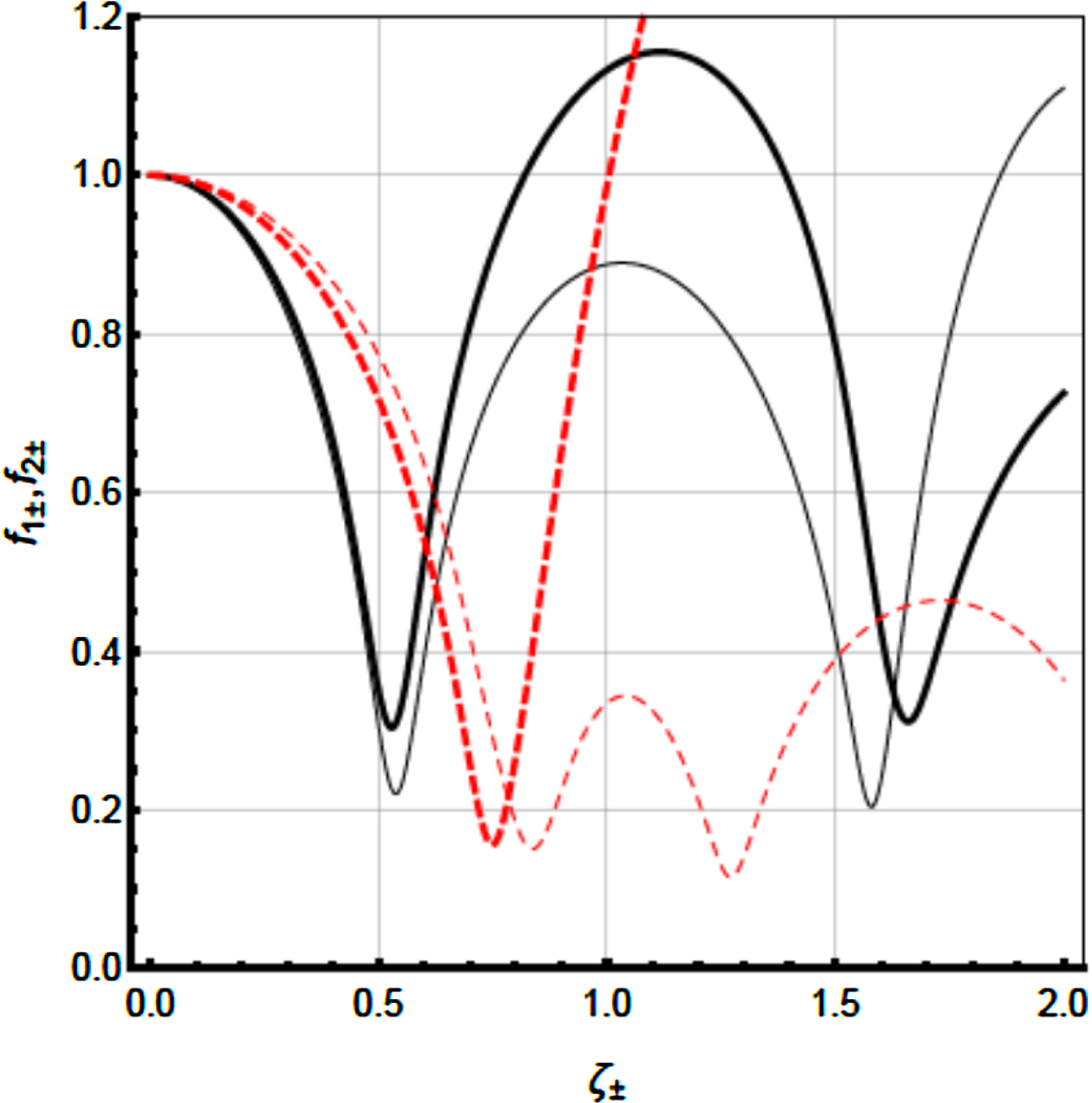
Figure 3 describes the variation of beam-width parameters f 1+ and f 2+ as a function of the dimensionless distance of propagation ζ+ for different values of decentered parameters b 1 and b 2 at a fixed value of equilibrium beam radius ρ01+ = ρ02+ = 4 and initial intensity parameter p 0+ = 0.5. It is obvious from the figure that for identical values of b 1 and b 2, f 1+ and f 2+ merge together as the beam propagates through the magnetized plasma. From solid curve for which b 1 = b 2 = 0, the circular symmetric nature of Gaussian beam is clear due to exact synchronized periodic oscillations of f 1+ and f 2+. Further, with an increase in decentered parameter in either or one dimension, strong self-focusing is observed with slight decrease in self-focusing length. This supports the earlier results (Gill et al., Reference Gill, Mahajan and Kaur2011, Reference Patil, Takale, Navare, Fulari and Dongare2012; Patil & Takale, Reference Patil and Takale2013; Nanda & Kant, Reference Nanda and Kant2014; Kant & Wani, Reference Kant and Wani2015) for self-focusing of circularly symmetric cosh-Gaussian beams in different situations. It is also interesting to note that complexity in oscillations of f 1+ and f 2+ occurs for different b values in x and y dimensions. It is quite apparent from this figure that after the initial focusing amplitude of oscillations of f 1+ (f 2+) increases (decreases) with an increase in b values in either dimensions. The reverse is also true for the next cycle of f 1+ and f 2+. The behaviors of f 1+ and f 2+ changes drastically but still maintains oscillatory self-focusing. Thus, increase in asymmetry in the beam by means of unlike decentering of beam profile in transverse dimensions of the beam results in large complexity in the oscillatory character of relevant beam-width parameters. Such complexity emanates due to coupled disturbed delicate balance between diffractional and non-linear terms in Eqs. (7) and (8).
Variation of the beam-width parameters f 1+ and f 2+ for E-mode with a dimensionless distance of propagation ζ+ with ρ01+,02+ = 4 and p 0+ = 0.5 for different decentered parameters in collisionless magnetized plasmas. Solid curve corresponds to decentered parameters b 1 = b 2 = 0.0, dashed curve corresponds to b 1 = 0.2 and b 2 = 0.6, dotted curve corresponds to b 1 = 0.4 and b 2 = 0.8. Thick curves are for f 1+ and thin curves are for f 2+. The other parameters are same as in Figure 2.

Figure 4 illustrates the dependence of beam-width parameters f 1+ and f 2+ as a function of thedimensionless distance of propagation ζ+ for different values magnetic field with b 1 = 0.4 and b 2 = 0.8. Oscillatory self-focusing is observed in Figure 4 where a decrease in the magnetic field leads to increase in self-focusing with a subsequent increase in self-focusing length. Such type of behavior is reasonably similar to the earlier prediction by Gill et al. (Reference Gill, Kaur and Mahajan2010) for the Gaussian beam. However, self-focusing is more in f 2+ as compared with f 1+. This is due to the slight higher value of the decentered parameter (b 2 = 0.8) in y dimension than x dimension where b 1 = 0.4.
Variation of the beam-width parameters f 1+ and f 2+ for E-mode with a dimensionless distance of propagation ζ+ with b 1 = 0.4 and b 2 = 0.8 for different static magnetic fields. Solid curve corresponds to a static magnetic field B 0 = 0.10 MG, dashed curve corresponds to B 0 = 0.15 MG, dotted curve corresponds to B 0 = 0.20 MG. Thick curves are for f 1+ and thin curves are for f 2+. The other parameters are same as in Figure 2.

The effect of polarization modes (E-mode and O-mode) on the behavior of beam-width parameters f 1± and f 2± with a dimensionless distance of propagation ζ± for B 0 = 0.10 MG with b 1 = 0.4 and b 2 = 0.8 has been presented in Figure 5. From this figure, it is obvious that both the modes show their clear propagation behavior of f 1± and f 2±. It is to be noted that significant self-focusing with increased focusing length is observed in case of ordinary mode than that of extraordinary mode. The complexity in behaviors of f 1± and f 2± in case of both the modes is noteworthy.
Variation of the beam-width parameters f 1± and f 2± with a dimensionless distance of propagation ζ± with b 1 = 0.4 and b 2 = 0.8 and B 0 = 0.10 MG. Solid curve corresponds to E-mode, while dashed curve corresponds to O-mode of polarization of laser. Thick curves are for f 1+ and thin curves are for f 2+. The other parameters are same as in Figure 2.
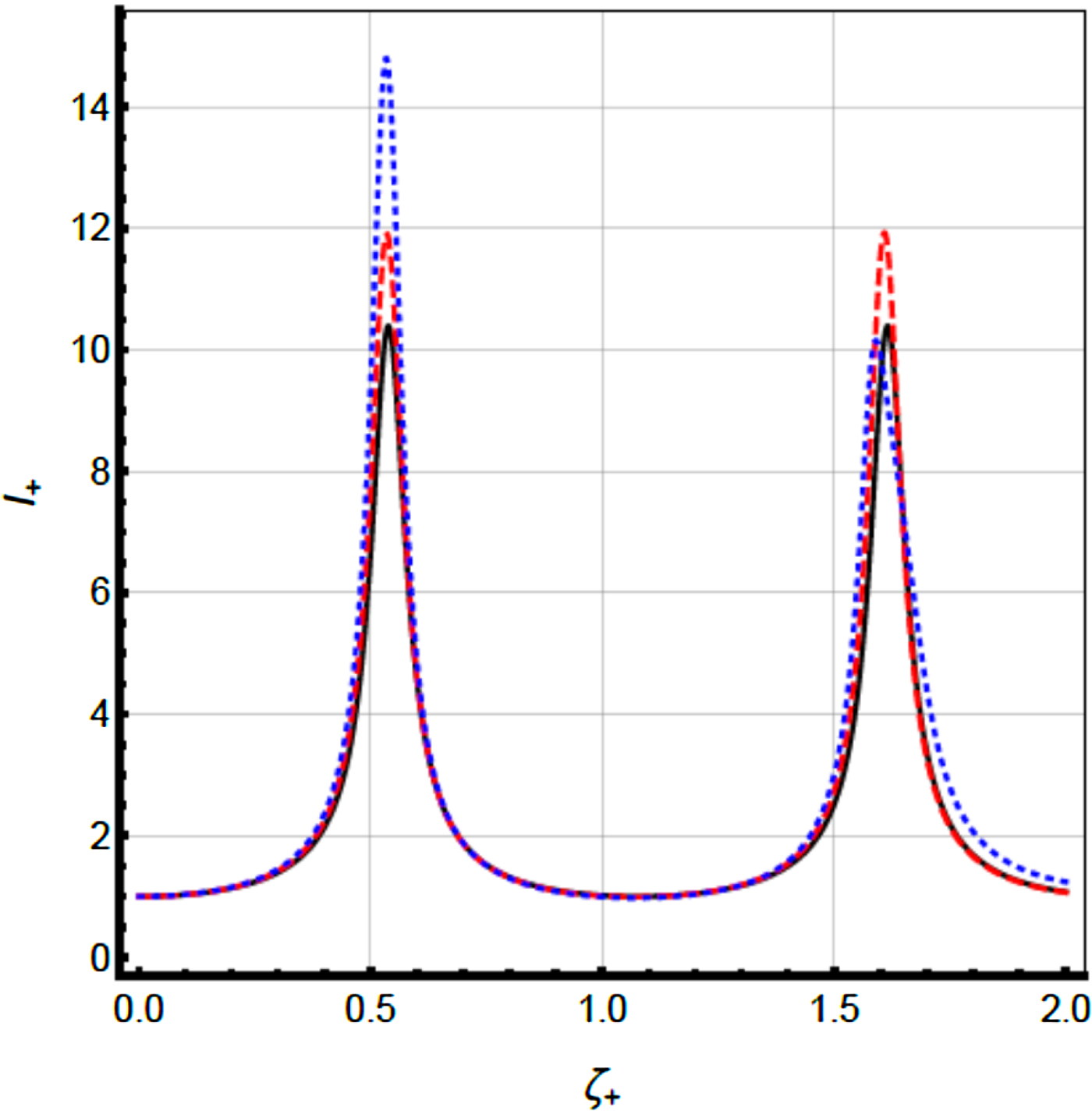
The behavior of f 1+ and f 2+ along ζ+ leads to an impact on laser beam intensity at same ζ+ values. Figure 6 elucidates the dependence of normalized axial beam intensity I + with ζ+ for three b values. As obvious, the normalized beam intensity shows oscillatory behavior which has gradual complexity along ζ+. As obvious, the oscillation peaks in I + corresponds to valleys of f 1+ and f 2+ with respective ζ+ values.
Dependence of the normalized axial beam intensity I + with dimensionless distance of propagation ζ+ for E-mode in collisionless magnetized plasmas. Solid curve corresponds to decentered parameters b 1 = b 2 = 0.0, dashed curve corresponds to b 1 = 0.2 and b 2 = 0.6, dotted curve corresponds to b 1 = 0.4 and b 2 = 0.8. The other parameters are same as in Figure 2.
4. CONCLUSION
In conclusion, an impact of decentered parameters on self-focusing of asymmetric cosh-Gaussian laser beams is studied by taking into account ponderomotive non-linearity in collisionless magnetized plasma. Following important conclusions are drawn from the present analysis:
-
• Self-focusing of laser beam increases with increase in decentered parameters in transverse dimensions of the beam.
-
• Symmetric self-focusing in transverse dimensions of the beam is possible for identical decentering of beam profile in both the dimensions.
-
• Complexity in self-focusing characters increases with increase in asymmetry through decentering the beam profile in both the dimensions of the beam.
-
• Change in the static magnetic field and polarization modes of laser offers a possible solution to study the complexity of beam propagation in transverse dimensions of the beam.
The present results may serve additional information in the various context of laser–plasma interaction, where laser beams with decentered irradiance distribution are requisite.



