



1. Introduction
In a wide range of nonlinear physics, various turbulent phenomena have been observed (Chaston et al. Reference Chaston, Salem, Bonnell, Carlson, Ergun, Strangeway and McFadden2008; Paoletti & Lathrop Reference Paoletti and Lathrop2011; Yang et al. Reference Yang, Jiang, Picano and Zhu2024). Turbulence is typically characterised by complex and irregular spatiotemporal evolution. In many cases, that motion is governed by deterministic equations, i.e. dynamical systems. Dynamical systems theory provides a unified approach to turbulent phenomena, viewing complex and irregular behaviour as arising from chaotic attractors in phase space. The three-dimensional (3-D) Navier–Stokes (NS) turbulence represents a significant example of high-dimensional chaos (Ruelle Reference Ruelle1989) and is the central focus of this study.
Sensitivity to initial conditions means that two arbitrarily close states diverge exponentially over time, which is the hallmark of chaos (Lorenz Reference Lorenz1995). Lyapunov analysis characterises the instability of infinitesimal perturbations evolving along orbits in phase space, where the exponential growth rate is quantified by the Lyapunov exponent and the corresponding direction by the Lyapunov vector. Formally, the Lyapunov exponents measure the rate of trajectory divergence in an infinite time limit and Oseledec’s multiplicative ergodic theory ensures the statistical well-defined nature of these time limits (Eckmann & Ruelle Reference Eckmann and Ruelle1985). The Lyapunov exponents and vectors represent local stability of chaotic trajectories in phase space, just like the eigenvalues and eigenvectors of steady states. The Lyapunov analysis reveals characteristics of chaotic dynamical systems, such as entropy, fractal dimension and hyperbolicity (Hirsch et al. Reference Hirsch, Smale and Devaney2012). However, while Lyapunov vectors are well-defined mathematically, their physical interpretation in spatially inhomogeneous turbulence remains unclear.
Meanwhile, NS turbulence can be characterised in terms of the transfer of kinetic energy from large-scale motions driven by forcing to small-scale dissipation due to viscosity (Davidson Reference Davidson2015). Numerical simulations and well-controlled experimental studies have revealed the existence of multiscale structures in developed turbulence. We can identify recurrent patterns in flow profiles, known as coherent structures, which may provide a clearer understanding of the spatiotemporal structure of turbulence. This paper investigates the turbulent motions underlying sensitivity to initial conditions.
On a 3-D torus in physical space, direct numerical simulation (DNS) of NS turbulence, also known as box turbulence, has been conducted in relation to homogeneous isotropic turbulence (HIT), which serves as a model for the statistical theory of turbulence (Frisch Reference Frisch1995). Ruelle (Reference Ruelle1979) suggested that the growth rate of infinitesimal perturbations in HIT satisfies the scaling based on Kolmogorov theory. In addition, Ruelle showed the distribution of the Lyapunov spectrum using the intermittent model (Frisch et al. Reference Frisch, Sulem and Nelkin1978; Ruelle Reference Ruelle1982). The degree of development of box turbulence is commonly characterised by the Taylor-microscale Reynolds number
 $R_\lambda$
. Kida & Ohkitani (Reference Kida and Ohkitani1992) carried out the Lyapunov analysis for high-symmetric turbulence at
 $R_\lambda =186$
and showed that the Lyapunov vector captures the small-scale perturbations around Kolmogorov-scale vortices, the smallest scale motions in NS turbulence.
Mohan et al. (Reference Mohan, Fitzsimmons and Moser2017) conducted a Lyapunov analysis of NS turbulence on a 3-D torus up to
 $R_\lambda =212$
. They showed that as the Reynolds number increases, the Lyapunov exponent increases slightly faster than the Kolmogorov scaling and the local Lyapunov vector characterises the instability of Kolmogorov-scale co-rotating vortex tubes. Ho et al. (Reference Ho, Armua and Berera2020) improved the dimensional analysis for the leading Lyapunov exponent, taking into account the Reynolds-number dependence of the dissipation rate, using turbulence data up to
 $R_\lambda =189$
. Ge et al. (Reference Ge, Rolland and Vassilicos2023) considered the finite-time growth of perturbations for box turbulence at
 $R_\lambda =152$
and supported the conclusions of Mohan et al. (Reference Mohan, Fitzsimmons and Moser2017). They suggested that large-scale sweep of the smallest-scale eddies violates the Kolmogorov scaling.
Furthermore, Boffetta & Musacchio (Reference Boffetta and Musacchio2017) conducted a finite-time Lyapunov analysis, which studies the separation of two orbits starting from very close initial conditions. The two orbits separate from small to large scales. After the initial exponential separation, the distance between two orbits increases algebraically over time. Berera & Ho (Reference Berera and Ho2018) also studied this problem setting and showed that the divergence of orbits grows at the same rate at all scales. Using the Gram–Schmidt orthogonalisation, Hassanaly & Raman (Reference Hassanaly and Raman2019) computed the Kaplan–Yorke dimension for low-Reynolds-number box turbulence. Regarding the orbital instability in two-dimensional turbulence (Nastac et al. Reference Nastac, Labahn, Magri and Ihme2017; Clark et al. Reference Clark, Tarra and Berera2020), Clark et al. (Reference Clark, Armua, Freeman, Brener and Berera2021) investigated a thin-periodic-box flow, which exhibits transitions from fully 3-D to 2-D turbulence. Changing the box height, they performed the Lyapunov analysis and found a discontinuous transition in the maximal Lyapunov exponent. Inubushi et al. (Reference Inubushi, Saiki, Kobayashi and Goto2023) considered the transverse Lyapunov exponent for characterising chaotic synchronisation in data assimilation.
Correspondingly, HIT has attracted considerable interest as a canonical flow for the statistical theory of turbulence. In contrast, wall-bounded turbulence is a prototypical example of inhomogeneous turbulence, characterised by strong spatial inhomogeneity and hierarchies of coherent structures. These fundamental differences raise the question of how orbital instability and Lyapunov vectors are organised in wall-bounded turbulence. Moreover, uncovering the essential mechanisms in wall-bounded turbulence is therefore a critical issue for engineering applications, e.g. drag reduction and mixing promotion. In laminar flow, the fluid motion is predominantly in the wall-parallel directions and wall-normal momentum transfer is made by molecular motion, whereas in turbulence, significant momentum transfer occurs in the wall-normal direction. The degree of development of wall-bounded turbulence is commonly characterised by the friction Reynolds number
 $h^+$
. As
 $h^+$
increases, a hierarchy of multiscale structures contributes substantially to momentum transport (Flores & Jiménez Reference Flores and Jiménez2010; Lozano-Duran & Jimenez Reference Lozano-Durán and Jiménez2014a
; Jiménez Reference Jiménez2018), further complicating the organisation of orbital instability.
On the sensitivity to initial conditions for wall-bounded turbulence, Keefe et al. (Reference Keefe, Moin and Kim1992) studied the Lyapunov spectrum of plane Poiseuille turbulence and found that the attractor dimension is 780 at
 $h^+=80$
. Inubushi et al. (Reference Inubushi, Takehiro and Yamada2015) conducted the covariant Lyapunov analysis (Ginelli et al. Reference Ginelli, Poggi, Turchi, Chaté, Livi and Politi2007) for Couette flow in a minimal flow unit (Hamilton et al. Reference Hamilton, Kim and Waleffe1995) which is small enough to contain a single coherent structure of the self-sustaining process (Jiménez & Moin Reference Jiménez and Moin1991; Waleffe Reference Waleffe1997). They demonstrated that the Lyapunov vectors associated with the positive Lyapunov exponents characterise the instability of streamwise vortices similar to the linear instability of model streaks (Schoppa & Hussain Reference Schoppa and Hussain2002; Kawahara et al. Reference Kawahara, Jiménez, Uhlmann and Pinelli2003). Ishikawa et al. (Reference Ishikawa, Takehiro and Yamada2018) applied Bloch’s theory to the Lyapunov analysis, using it to study subharmonic instability related to the oblique pattern during subcritical transition to Couette turbulence. These studies concern near-wall dynamics in nearly minimal settings at
 $h^+\leqslant 40$
. Nikitin and his co-workers performed time integration of the linearised NS equations for wall-bounded turbulence at higher
 $h^+$
, up to 586 (Nikitin Reference Nikitin2008, Reference Nikitin2009, Reference Nikitin2018; Nikitin & Pivovarov Reference Nikitin and Pivovarov2018; Nikitin & Popelenskaya Reference Nikitin and Popelenskaya2019), and studied infinitesimal perturbations starting from random initial conditions. The majority of perturbations in the finite-time growth process occurs in the buffer layer, where its characteristic streamwise and spanwise lengths are, on average, half those of the minimal flow unit. These previous studies motivate us to consider moderately developed Couette turbulence up to
 $h^+=269$
as an intermediate regime beyond the minimal flow unit, as a step towards understanding orbital instability in fully developed wall turbulence. This regime contains small-to-large-scale structures that are not accommodated by a minimal flow unit, while remaining computationally tractable through the long-time integrations required for Lyapunov analysis.
This paper performs a Lyapunov analysis of moderately developed Couette turbulence to elucidate the relationship between coherent structures and orbital instability. Long-time Lyapunov analysis shows that the leading Lyapunov exponent appears to follow the wall-unit scaling and that the corresponding Lyapunov vector is predominantly supported in the buffer layer, with characteristic scales smaller than the minimal flow unit. Using coarse graining with a Gaussian low-pass filter, we further show that the vortical structures of the local Lyapunov vector are wrapped around large-scale quasi-streamwise vortices near the wall. These results suggest that orbital instability in wall-bounded turbulence is governed by small-scale perturbations sustained by the prominent strain induced by near-wall large-scale vortices. The problem set-up and the results are presented in §§ 2 and 3, respectively, and concluding remarks are given in § 4.
2. Set-up
We consider plane Couette flow where an incompressible fluid is confined between two parallel walls moving in opposite tangential directions. The motion of the unit-density fluid is governed by the NS equations:
 \begin{align} \boldsymbol{\nabla }\boldsymbol{\cdot }\boldsymbol{u}=0, \quad \frac {\partial \boldsymbol{u}}{\partial t} + (\boldsymbol{u}\boldsymbol{\cdot }\boldsymbol{\nabla })\boldsymbol{u}=-\boldsymbol{\nabla }p +\nu {\nabla} ^2 \boldsymbol{u}. \end{align}
Here,
 $t$
denotes time;
 $x_i$
 $(i=1,2,3)$
stand for streamwise, wall-normal and spanwise directions, respectively;
 $u_i(\boldsymbol{x},t)$
 $(i=1,2,3)$
are the components of the velocity
 $\boldsymbol{u}$
in the
 $x_i$
-direction;
 $p$
is the pressure and
 $\nu$
signifies the kinematic viscosity. The distance between the walls is
 $2h$
and the speed difference is
 $2U$
. The Reynolds number is defined as
 $R= \textit{Uh}/\nu$
.
We impose periodic boundary conditions in the streamwise
 $x_1$
and spanwise
 $x_3$
directions with the periods
 $L_1$
and
 $L_3$
, while the non-slip and impermeability conditions are imposed at the walls,
 $\left .\boldsymbol{u}\right |_{x_2=\pm h}=(\pm U,0,0)$
. The Chebyshev–Fourier–Galerkin spectral method is employed for space discretisation, where the number of grid points
 $(N_1, N_2, N_3)$
increases following the recent DNS for Couette turbulence performed by Lee & Moser (Reference Lee and Moser2018). The truncation mode numbers
 $M_i$
 $(i=1,2,3)$
satisfy
 $N_1\geqslant 3M_1+1, N_2\geqslant 2M_2, N_3\geqslant 3M_3+1$
to eliminate the aliasing error.
We apply the second-order Crank–Nicolson and Adams–Bashforth methods for time evolution and perform DNS with the streamwise and spanwise period of the domain fixed at
 $(L_1, L_3)=(2\pi h, \pi h)$
or at
 $(L_1^+, L_3^+)\simeq (400, 100)$
. Here, the superscript
 $^+$
denotes the wall unit as determined through the non-dimensionalisation using the friction velocity
 $u_\tau$
and the kinematic viscosity. The latter domain has a slightly longer streamwise period compared with the minimal flow unit
 $250 \leqslant L_1^+\leqslant 350, L_3^+\simeq 100$
presented by Jiménez & Moin (Reference Jiménez and Moin1991) for channel turbulence. For simplicity, we hereafter refer to the domain size
 $(L_1^+, L_3^+)\simeq (400,100)$
as the minimal flow unit. Table 1 presents details of the numerical set-up. While much larger domains would be desirable for assessing domain-size effects, they are computationally demanding for the long-time integrations required by Lyapunov analysis.
Numerical set-up. Here,
 $ R=Uh/\nu$
and
 $ h^+=u_\tau h/\nu$
are the Reynolds number and the friction Reynolds number, respectively.
 $(L_1^+, L_3^+)$
denotes the streamwise and spanwise periods of the computational domain in wall units, and
 $N_i(i=1, 2, 3)$
represents the number of grid points in the streamwise, wall-normal and spanwise directions.
 $T_{{ave}}u_\tau /h$
signifies the averaging time, while
 $\langle \overline {\gamma ^1} \rangle \pm \sigma _{\overline {\gamma ^1}}$
and
 $\sigma _{\gamma ^1}$
stand for the ensemble-averaged Lyapunov exponent with its standard deviation and the standard deviation of the local Lyapunov exponent, respectively. The domain size of the former three cases is
 $(L_1, L_3)=(2\pi h, \pi h)$
.

Table 1. Long description
A table with 6 rows and 9 columns comparing numerical set-up details for different Reynolds numbers. The columns are labeled R, h+, (L1+, L3+), (N1, N2, N3), Taveu+/h, [(γ-^γ) ± σγγ]/h/U, and σγγ/h/U. The rows present data for different Reynolds numbers (R) and their corresponding values. Row 1: R 1000, h+ 66.3, (L1+, L3+) (416, 208), (N1, N2, N3) (96, 96, 96), Taveu+/h 4640, [(γ-^γ) ± σγγ]/h/U 0.102 ± 3.76 × 10^-4, σγγ/h/U 3.42 × 10^-2. Row 2: R 3000, h+ 171, (L1+, L3+) (1074, 537), (N1, N2, N3) (128, 160, 128), Taveu+/h 1420, [(γ-^γ) ± σγγ]/h/U 0.233 ± 6.06 × 10^-3, σγγ/h/U 5.54 × 10^-2. Row 3: R 5000, h+ 269, (L1+, L3+) (1690, 845), (N1, N2, N3) (160, 192, 160), Taveu+/h 1340, [(γ-^γ) ± σγγ]/h/U 0.393 ± 1.23 × 10^-3, σγγ/h/U 9.67 × 10^-2. Row 4: R 1200, h+ 72.8, (L1+, L3+) (457, 114), (N1, N2, N3) (96, 96, 48), Taveu+/h 1820, [(γ-^γ) ± σγγ]/h/U 0.122 ± 4.27 × 10^-4, σγγ/h/U 3.67 × 10^-2. Row 5: R 3100, h+ 147, (L1+, L3+) (462, 115), (N1, N2, N3) (96, 192, 48), Taveu+/h 710, [(γ-^γ) ± σγγ]/h/U 0.193 ± 6.13 × 10^-4, σγγ/h/U 4.85 × 10^-2. Row 6: R 8000, h+ 266, (L1+, L3+) (418, 104), (N1, N2, N3) (96, 256, 48), Taveu+/h 400, [(γ-^γ) ± σγγ]/h/U 0.256 ± 1.04 × 10^-3, σγγ/h/U 5.96 × 10^-2.
For the Lyapunov analysis, we introduce a time-
 $T$
map, which simply advances a given flow state by a fixed time interval
 $T$
. Formally, the time-
 $T$
map
 $\phi _T(\xi )$
is defined by the time integration of the NS equations up to time
 $T$
from the initial condition
 $\xi$
, where
 $\xi \in \mathbb{R}^D$
 $(D=4(2M_1+1)(M_2-2)(2M_3+1)+2(M_2-2))$
denotes the state variable composed of the real and imaginary parts of the spectral coefficients of the toroidal and poloidal potentials for the velocity field.
Infinitesimal perturbations follow the linearised NS equations. To track the time evolution of perturbations along the trajectory in phase space, we consider the discrete maps for the reference state
 $\xi _n$
and the perturbation
 $\delta \xi _n^1$
as follows:
 \begin{align} \xi _{n+1}=\phi _T(\xi _n), \quad \delta \xi _{n+1}^1=\frac {\partial \phi _T(\xi _n)}{\partial \xi }\delta \xi _n^1, \end{align}
where
 $\partial \phi _T(\xi )/\partial \xi$
is the Jacobian matrix of the time-
 $T$
map. In other words, this Jacobian advances an infinitesimal perturbation along the reference trajectory over the time interval
 $T$
according to the linearised NS equations. After sufficiently long-time integration, the perturbation
 $\delta \xi _n^1$
describes the least stable direction for the state
 $\xi _n$
. The first Lyapunov exponent is defined as the time-averaged exponential growth rate of the most unstable perturbation:
 \begin{align} \overline {\gamma ^1}=\lim _{n\rightarrow \infty } \frac {1}{nT}\ln \frac {||\delta \xi _n^1||}{||\delta \xi _0^1||}. \end{align}
Here,
 $||\boldsymbol{\cdot }||$
represents the energy (
 $L^2$
) norm of the velocity field in physical space reconstructed from the spectral coefficients, while
 $\delta \xi _0^1$
is the initial condition of perturbation. The denominator
 $||\delta \xi _0^1||$
makes the argument of the logarithm dimensionless and its contribution to the Lyapunov exponent vanishes in the long-time limit.
If the first Lyapunov exponent
 $\overline {\gamma ^1}$
is positive, the dynamical system exhibits the sensitivity to initial conditions (Hirsch et al. Reference Hirsch, Smale and Devaney2012). To characterise the instability along the orbit, we consider the first local Lyapunov exponent:
 \begin{align} \gamma _n^1=\frac {1}{T}\ln \frac {||\delta \xi _{n+1}^1||}{||\delta \xi _n^1||}, \end{align}
which represents the exponential growth rate of perturbation
 $\delta \xi _n^1$
over the time interval
 $T$
. The corresponding perturbation
 $\delta \xi _n^1$
is referred to as the first local Lyapunov vector. In addition, the first Lyapunov exponent can be expressed as
 \begin{align} \overline {\gamma ^1}=\lim _{n\rightarrow \infty }\frac {1}{n}\sum _{m=1}^n \gamma _m^1. \end{align}
Hereafter, we simply refer to them as the Lyapunov exponent and the (local) Lyapunov vector. After evaluating the local Lyapunov exponent, we rescale each local Lyapunov vector so that
 $||\delta \xi _n^1||/U=1$
and compute statistics such as the root-mean-square (r.m.s.) velocity profiles. For visual comparison of their spatial distributions across Reynolds numbers and domain sizes, the velocity components of these rescaled vectors are divided by
 $u_\tau$
of the corresponding turbulent state. We stress that the perturbation
 $\delta \xi _n^1$
is defined up to a multiplicative constant (Inubushi et al. Reference Inubushi, Takehiro and Yamada2015; Nikitin Reference Nikitin2018). Therefore, the absolute magnitudes of the resulting profiles have no physical meaning; only their spatial distributions and relative localisation are discussed.
We generate ten different initial conditions for turbulent orbits at each Reynolds number to compute the ensemble average. These different orbits also enable us to assess the dependence of the computed Lyapunov statistics on the reference turbulent trajectory. We carry out time integration up to
 $T_{{ave}}u_\tau /h\gt 10^3$
to take time averages, after discarding an initial transient of approximately
 $10^2h/u_\tau$
. In the case of
 $h^+=269$
and
 $(L_1,L_3)=(2\pi h,\pi h)$
, for example, the averaging time is
 $T_{{ave}}=2.5\times 10^4h/U$
, which is approximately
 $3.6\times 10^5$
wall-unit time measured in
 $\nu /u_\tau ^2$
.
Nikitin and his co-workers examined the perturbation growth for wall-bounded turbulence (Nikitin Reference Nikitin2008, Reference Nikitin2009, Reference Nikitin2018; Nikitin & Pivovarov Reference Nikitin and Pivovarov2018; Nikitin & Popelenskaya Reference Nikitin and Popelenskaya2019). Their time integration extended to approximately
 $20 h/u_\tau$
, although the domain size for Couette turbulence of Nikitin & Pivovarov (Reference Nikitin and Pivovarov2018) is larger than ours. These studies considered the finite-time evolution of random perturbations governed by the linearised NS equations. As implied by the above-mentioned definition of the Lyapunov exponent, the dependence on the initial perturbation disappears only in the long-time limit. Thus, while these pioneering studies provide important information on disturbance growth in wall-bounded turbulence, they do not directly determine the asymptotic Lyapunov vector considered in the present work. Therefore, we compute the asymptotic Lyapunov exponent and the corresponding Lyapunov vector through long-time integration.
The perturbation is renormalised every time interval
 $T$
, which we fix at
 $T=1h/U$
. Using
 $T=0.1h/U$
and
 $10h/U$
, we have confirmed that the results presented in this paper do not depend on the choice of the time interval of the normalisation. The Lyapunov spectrum and the corresponding Lyapunov vectors can be obtained from numerical computation, which is similar to that for the eigenvalue problem of linear stability analysis for steady states. See Ginelli et al. (Reference Ginelli, Chaté, Livi and Politi2013) for detailed descriptions of the Lyapunov analysis.
(a) Mean velocity
 $U_1^+$
as a function of the wall-unit distance from the wall
 $y^+$
. The blue, green and red lines correspond to
 $h^+=66.3,\,171$
and 269 with
 $(L_1, L_3)=(2\pi h, \pi h)$
, while the black line is produced by Lee & Moser (Reference Lee and Moser2018) at
 $h^+=501$
with
 $(L_1, L_3)=(100\pi h, 5\pi h)$
. (b) Streamwise r.m.s. velocity
 $u_1'^+$
. The definition of lines is the same as in panel (a), but the blue pluses, green crosses and red circles indicate the corresponding quantities of the energy-normalised Lyapunov vector
 $\delta u_1'/u_\tau$
at
 $h^+=66.3,\, 171$
and 269.

Figure 1 shows the mean and r.m.s. velocity profiles of our domain size, serving to verify our numerical computation. The mean velocity profile is in good agreement with that of developed turbulence reported by Lee & Moser (Reference Lee and Moser2018). In contrast to the large-domain simulation, however, the maxima of the r.m.s. velocity decrease slightly with increasing the Reynolds number due to the restriction on domain size for large-scale structures. Although the domain size is too small to capture large-scale motions in Couette turbulence, this study provides a perspective on turbulence from the viewpoint of dynamical systems theory. Hereafter, we denote time-averaged and ensemble-averaged values of
 $a$
as
 $\overline {a}$
and
 $\langle a\rangle$
, respectively.
3. Results
Figure 2 shows the asymptotic behaviour of the (first) Lyapunov exponent
 $\overline {\gamma ^1}$
in the domain
 $(L_1, L_3) = (2\pi h, \pi h)$
as a function of the averaging time
 $T_{{ave}} u_\tau / h$
. The Lyapunov exponents computed from ten independent turbulent trajectories seem to converge to a particular value after sufficiently long-time averaging, up to approximately
 $T_{{ave}} u_\tau / h \simeq 10^3$
. The differences among the Lyapunov exponents across the ten trajectories are within 1 % relative error at each Reynolds number. This result suggests that long-time averaging is essential to accurately determine the Lyapunov exponent.
Lyapunov exponent in
 $(L_1,L_3)=(2\pi h,\pi h)$
as a function of the averaging time
 $T_{ {ave}}u_\tau /h$
. The horizontal black lines represent the ensemble-averaged Lyapunov exponent
 $\langle \overline {\gamma ^1}\rangle h/U=0.102,0.233,$
and 0.393 at
 $h^+=66.3,\, 171$
and 269, respectively. The grey lines represent the Lyapunov exponent for each turbulent orbit at different Reynolds numbers. The red and blue lines signify the first and second Lyapunov exponents obtained by the Schmidt–Lyapunov analysis at
 $h^+=171$
, where
 $\overline {\gamma ^1}=0.233U/h$
and
 $\overline {\gamma ^2}=0.230U/h$
at
 $T_{{ave}}u_\tau /h=2840$
.

The ensemble-averaged Lyapunov exponents and the standard deviation of the local Lyapunov exponents are summarised in table 1. As expected, both the Lyapunov exponent and the fluctuation increase monotonically with the Reynolds number, consistent with previous findings in box turbulence by Mohan et al. (Reference Mohan, Fitzsimmons and Moser2017). Moreover, Nikitin & Pivovarov (Reference Nikitin and Pivovarov2018) reported, using time integration of the linearised NS equations for Couette turbulence at
 $h^+ = 121$
in a larger domain
 $(L_1, L_3) = (10h, 5h)$
, that the most unstable Lyapunov exponent is approximately
 $0.16 U/h$
, which is comparable with our results.
The Lyapunov exponents characterise the exponential instability along a turbulent orbit in phase space. One may naively expect that the Lyapunov exponent is governed by the fastest time scale in the dynamical system. For wall-bounded turbulence, the near-wall structures represent the smallest-scale motions and the wall unit defines the fastest time scale. Note that in the near-wall region, the Kolmogorov time scale evaluated with the local energy dissipation on the wall is consistent with the friction time scale
 $\nu /u_\tau ^2$
; however, in the core region, the local Kolmogorov time scale is larger than
 $\nu /u_\tau ^2$
because the local energy dissipation therein is smaller. Therefore, using the reciprocal of the friction time scale, one may estimate the Lyapunov exponent as
 $\overline {\gamma } \sim u_\tau ^2 / \nu$
.
Figure 3(a) presents the ensemble-averaged Lyapunov exponent non-dimensionalised by
 $h/u_\tau$
. As the friction Reynolds number
 $h^+$
increases, the Lyapunov exponent increases as
 $\overline {\gamma } h / u_\tau \sim h^+ = u_\tau h / \nu$
, suggesting that our result in figure 3(a) is consistent with the above-mentioned friction-time scale estimate. This implies that
 $\gamma ^+=\overline {\gamma }/(u_\tau ^2/\nu )$
is approximately constant. The least-squares fits in figure 3(a) give
 $\gamma ^+\approx 0.0285$
for the larger domain and
 $\gamma ^+\approx 0.0295$
for the minimal flow unit. Nikitin (Reference Nikitin2008) and Nikitin (Reference Nikitin2009) reported
 $\gamma ^+\approx 0.021$
for pipe and plane channel flows, while Nikitin & Pivovarov (Reference Nikitin and Pivovarov2018) obtained
 $\gamma ^+\approx 0.023$
for Couette flow at several Reynolds numbers. Nikitin (Reference Nikitin2018) also showed
 $\gamma ^+\approx 0.026$
for channel turbulence at
 $h^+=586$
. Thus, the present values are somewhat larger than, but remain comparable to, the previous values obtained by finite-time disturbance-growth calculations.
(a) Ensemble-averaged Lyapunov exponents. The red points and blue circles correspond to
 $(L_1, L_3)=(2\pi h, \pi h)$
and the minimal flow unit, respectively. The open circle at
 $(h^+,\overline {\gamma }h/u_\tau )=(34.0,0.021)$
is reproduced from Inubushi et al. (Reference Inubushi, Takehiro and Yamada2015) at
 $R=400$
in
 $(L_1,L_3)=(1.755\pi h,1.2\pi h)$
, which is the minimal flow unit at this Reynolds number (Hamilton et al. Reference Hamilton, Kim and Waleffe1995). The red and blue dashed lines are obtained by the least-squares fits to our results:
 $\overline {\gamma } h / u_\tau \sim 0.0285 h^+$
for the domain
 $(L_1, L_3) = (2\pi h, \pi h)$
and
 $\overline {\gamma } h / u_\tau \sim 0.0295 h^+$
for the minimal flow unit. (b) Probability density function of the local Lyapunov exponent
 $\gamma _n^1$
rescaled by the standard deviation
 $\sigma _{\gamma ^1}$
. The lines correspond to
 $(L_1, L_3)=(2\pi h,\pi h)$
, while pluses, crosses and circles represent the minimal flow units. As the Reynolds number increases, the colour changes from blue to green to red.

In contrast, for HIT, the smallest eddies, i.e. the Kolmogorov-scale motions, provide the fastest time scale and one may therefore expect the leading Lyapunov exponent to be related to that time scale. Mohan et al. (Reference Mohan, Fitzsimmons and Moser2017), however, performed Lyapunov analysis for box turbulence and reported that the Lyapunov exponent increases even faster than the Kolmogorov scaling for HIT, following
 $\overline {\gamma } \sim (\varepsilon /\nu )^{1/2}$
as proposed by Ruelle (Reference Ruelle1979), where
 $\varepsilon$
is the energy dissipation rate.
Accordingly, within the range of Reynolds numbers examined in the present study, the Lyapunov exponents appear to follow the wall-unit (or near-wall Kolmogorov) scaling; however, the validity of this relationship at higher Reynolds numbers remains unclear due to the limited Reynolds number range. Lyapunov analysis with sufficiently long-time integration at high Reynolds numbers is required to clarify the scaling properties in fully developed turbulence. However, in the minimal flow unit, the rescaled Lyapunov exponent
 $\overline {\gamma } h / u_\tau$
is slightly larger than that in the domain
 $(L_1,L_3)=(2\pi h,\pi h)$
. We revisit these results later.
Figure 3(b) shows the probability density function (p.d.f.) of the local Lyapunov exponents. The skewness is positive, although its dependence on Reynolds number is non-trivial. In the case of minimal flow units, the p.d.f.s nearly overlap. Ho et al. (Reference Ho, Armua and Berera2020) performed a finite-time Lyapunov analysis of box turbulence and concluded that the p.d.f. of the local Lyapunov exponents follows a Gaussian distribution. To study subharmonic instability related to the oblique pattern in Couette flow, Ishikawa et al. (Reference Ishikawa, Takehiro and Yamada2018) considered orbital instability by applying Bloch’s theory in their Lyapunov analysis. They reported that the p.d.f. of the local Lyapunov exponent follows a Gaussian distribution.
Our results show that the p.d.f. of the local Lyapunov exponent exhibits deviations from Gaussian behaviour at higher Reynolds numbers. We also note that the p.d.f. in the minimal flow unit appears to follow a Gaussian distribution regardless of the Reynolds number, whereas the p.d.f. in the larger domain
 $(L_1, L_3) = (2\pi h, \pi h)$
shows a clear Reynolds-number dependence. These observations suggest that large-scale structures present in the larger domain may bring about the Reynolds-number dependence of the Lyapunov exponents.
As shown in figure 3(b), the Lyapunov exponents depend on the domain size, indicating that specific flow structures lead to instability. In figure 1(b), we plot the streamwise r.m.s. velocity profiles of the Lyapunov vector. The Lyapunov vector exhibits prominent fluctuations in the buffer layer. As the Reynolds number increases, the r.m.s. profile becomes more strongly concentrated in the buffer layer relative to the core region. This result indicates that the buffer layer dynamics dominate the orbital instability in developed wall turbulence.
Figure 4 presents the r.m.s. velocity of the Lyapunov vector. For the domain size
 $(L_1,L_3)=(2\pi h,\pi h)$
, as the Reynolds number increases, the peak of the r.m.s. velocity shifts towards the walls, while its magnitude in the core region decreases. These results further suggest that most of the least stable perturbations in wall turbulence are concentrated within the buffer layer.
Meanwhile, in the minimal flow unit, the r.m.s. velocity maintains an almost constant magnitude in the core region. This behaviour indicates that the Lyapunov vector captures the instability of the eddies detached from the wall, referred to as secondary vortices (Jiménez & Pinelli Reference Jiménez and Pinelli1999). As shown in figure 3(a), the Lyapunov exponents in the minimal flow unit are slightly larger than those in the
 $(L_1,L_3)=(2\pi h,\pi h)$
domain; this difference may arise from the instability of the secondary vortices. In addition, the r.m.s. velocity profiles of the Lyapunov vector exhibit mirror symmetry with respect to the midplane of the channel.
R.m.s. velocity profiles of the Lyapunov vector: (a)
 $\delta u'_2/u_\tau$
; (b)
 $\delta u'_3/u_\tau$
. The left-hand halves display
 $(L_1,L_3)=(2\pi h,\pi h)$
, and the right-hand halves display the minimal flow unit. The lines correspond to
 $(L_1, L_3)=(2\pi h,\pi h)$
, while pluses, crosses and circles represent the minimal flow unit. As the Reynolds number increases, their colour changes from blue to green to red.

Figure 4. Long description
Two line graphs depict velocity profiles of the Lyapunov vector. Panel A and Panel B each show two halves: the left-hand halves display the Lyapunov vector, and the right-hand halves display the minimal flow unit. The x-axis is labeled x2/h, and the y-axis is labeled with delta u2/utau for Panel A and delta u3/utau for Panel B. The lines correspond to different Reynolds numbers, with colors changing from blue to green to red as the Reynolds number increases. Pluses, crosses, and circles represent the minimal flow unit.
Time-averaged 1-D pre-multiplied energy spectra of turbulence at
 $h^+=269$
: (a)
 $k_1E_{11}$
and (b)
 $k_3E_{22}$
. The blue pluses and crosses stand for the buffer layer at
 $y^+=30.0$
and 61.6, while the red points and triangles indicate the core region at
 $y/h=0.65$
and 1.0. Here,
 $y=h-x_2$
denotes the distance from the wall at
 $x_2=h$
.

The r.m.s. velocity of the Lyapunov vector suggests that near-wall motions dominate the instability in developed wall-bounded turbulence. To examine the wall-parallel structures, we study the time-averaged one-dimensional (1-D) pre-multiplied energy spectra given by
 $k_1 E_{11} = k_1 \overline {\sum _{k_3} |\hat {u}_1|^2/2}$
and
 $k_3 E_{22} = k_3 \overline {\sum _{k_1} |\hat {u}_2|^2/2}$
for the streamwise and wall-normal velocity components. Here,
 $\hat {u}_1 = \hat {u}_1(t, k_1, x_2, k_3)$
and
 $\hat {u}_2 = \hat {u}_2(t, k_1, x_2, k_3)$
are the Fourier coefficients of the streamwise and wall-normal velocities, where
 $k_1$
and
 $k_3$
denote the streamwise and spanwise Fourier wavenumbers. Accordingly, the corresponding wavelengths are
 $\lambda _1^+ = L_1^+ / k_1$
and
 $\lambda _3^+ = L_3^+ / k_3$
.
Figure 5 presents the 1-D pre-multiplied energy spectra of the reference state at
 $h^+ = 269$
. They have significant structures near the walls, with a spanwise scale of
 $\lambda _3^+\simeq 100$
. Jiménez & Moin (Reference Jiménez and Moin1991) showed that the wall-parallel domain requires approximately
 $250 \leqslant L_1^+ \leqslant 350$
and
 $L_3^+ \simeq 100$
to sustain plane Poiseuille turbulence. In this domain, known as the minimal flow unit, turbulence undergoes a self-sustaining process that involves the generation and breakdown of streaks (Waleffe Reference Waleffe1997). The self-sustaining process constitutes the dominant coherent motion near the walls in wall-bounded turbulence. The 1-D pre-multiplied energy spectra shown in figure 5 demonstrate the approximate universality of small-scale near-wall turbulence, as previously reported (Avsarkisov et al. Reference Avsarkisov, Hoyas, Oberlack and García-Galache2014; Lee & Moser Reference Lee and Moser2018).
Figure 6 displays the 1-D pre-multiplied energy spectra of the Lyapunov vector, representing the least stable perturbation, at
 $h^+ = 269$
. We find that the 1-D energy spectra
 $k_1 \delta E_{11}$
and
 $k_3 \delta E_{22}$
exhibit maxima at
 $\lambda _1^+ \simeq 100$
and
 $\lambda _3^+ \simeq 50$
in the buffer layer, and we obtain similar spectra at the lower Reynolds numbers. Figure 7 plots
 $k_1 \delta E_{11}$
and
 $k_3 \delta E_{22}$
in the buffer layer for all of the Reynolds numbers and domain sizes. Regardless of the domain size and Reynolds number, the spectra show maxima at
 $\lambda _1^+ \simeq 100$
and
 $\lambda _3^+ \simeq 50$
. Therefore, the least stable perturbation exhibits ubiquitous structures with streamwise and spanwise scales of approximately 100 and 50 wall units, respectively, in the buffer layer.
Nikitin and his co-workers reported that, in the finite-time growth of random perturbations, the dominant perturbation energy is concentrated in the buffer layer and that its characteristic scales are smaller than those of the corresponding structures in the base flow (Nikitin Reference Nikitin2008, Reference Nikitin2009, Reference Nikitin2018; Nikitin & Pivovarov Reference Nikitin and Pivovarov2018; Nikitin & Popelenskaya Reference Nikitin and Popelenskaya2019). Although their analysis was based on finite-time perturbation growth rather than asymptotic Lyapunov vectors, their observations are consistent with the support and characteristic scales of the leading Lyapunov vector obtained here.
Time-averaged 1-D pre-multiplied energy spectra of the Lyapunov vector at
 $h^+=269$
: (a)
 $k_1\delta E_{11}$
and (b)
 $k_3\delta E_{22}$
. The definitions of points and colours follow those in figure 5.

Figure 6. Long description
Two scatter plots depict time-averaged 1-D pre-multiplied energy spectra of the Lyapunov vector. Panel A: The scatter plot shows the energy spectra on the vertical axis labeled k1δE11/uτ^2 and the horizontal axis labeled λ1+. Different symbols and colors represent various data points. Panel B: The scatter plot shows the energy spectra on the vertical axis labeled k3δE22/uτ^2 and the horizontal axis labeled λ3+. Different symbols and colors represent various data points.
Time-averaged 1-D pre-multiplied energy spectra of the Lyapunov vector in the buffer layer: (a)
 $k_1\delta E_{11}$
and (b)
 $k_3\delta E_{22}$
. The lines correspond to
 $(L_1, L_3)=(2\pi h,\pi h)$
, while pluses, crosses and circles represent the minimal flow unit. As the Reynolds number increases, their colour changes from blue to green to red.

In the buffer layer, a self-sustaining process involving the generation and breakdown of streaks can be identified. The self-sustaining streak dynamics can be characterised by streak instability (Schoppa & Hussain Reference Schoppa and Hussain2002; Kawahara et al. Reference Kawahara, Jiménez, Uhlmann and Pinelli2003). If the streak instability in the buffer layer triggers the orbital instability for wall-bounded turbulence, the least stable perturbation would be expected to have the minimal flow unit scale, i.e. approximately 400 streamwise and 100 spanwise wall units. However, the majority of the least stable perturbations are smaller than the minimal flow unit. Therefore, smaller-scale motions of turbulence are excited by the disturbance field. Our results appear contradictory because the prominent structures of the Lyapunov vector are too small relative to the minimal flow unit, where the self-sustaining process provides the fastest time scale for wall-bounded turbulence. As will be discussed later, this apparent contradiction may be resolved if the leading Lyapunov exponents are nearly degenerate, so that the orbital instability in the buffer layer is associated with a nearly degenerate set of small-scale perturbation directions rather than with a single minimal-unit-scale structure.
To estimate the second Lyapunov exponent in practice, we evolve a second perturbation together with the leading one. Since the second perturbation also tends to align with the most unstable direction, we remove its component parallel to the first Lyapunov vector after each renormalisation step. The growth rate of the remaining orthogonal component defines the second Lyapunov exponent. To formalise this procedure, we conduct the Schmidt–Lyapunov analysis to study the secondary unstable growth rate (Benettin et al. Reference Benettin, Galgani and Strelcyn1976; Shimada & Nagashima Reference Shimada and Nagashima1979). This procedure can be expressed in terms of the expansion rate of the area spanned by two orthogonal perturbation vectors
 $\delta \xi _n^1$
and
 $\delta \xi _n^2$
, where
 $\delta \xi _n^1 \perp \delta \xi _n^2$
. From this expansion rate, we can obtain the second Lyapunov exponent, representing the growth rate of the secondary unstable perturbation. The expansion rate of the area is given by
 \begin{align} \overline {\gamma ^1}+\overline {\gamma ^2}=\lim _{n\rightarrow \infty } \frac {1}{nT}\ln \big\|\delta \xi _n^1\wedge \delta \xi _n^2 \big\|, \end{align}
where
 $\overline {\gamma ^2}$
denotes the second Lyapunov exponent satisfying
 $\overline {\gamma ^1} \geqslant \overline {\gamma ^2}$
and
 $\wedge$
denotes the outer product.
The secondary perturbation
 $\delta \xi _n^2$
also obeys the linearised NS equations. Hence, the time evolution of
 $\delta \xi _n^2$
over the time interval
 $T$
is also given by the Jacobian of the time-
 $T$
map. Notably,
 $(\partial \phi _T/\partial \xi )\delta \xi _n^2$
generally has a component along the most unstable direction, i.e. the first local Lyapunov vector
 $\delta \xi _{n+1}^1$
, in addition to the secondary unstable direction. Therefore, we apply the Gram–Schmidt orthogonalisation to
 $ (\partial \phi _T / \partial \xi ) \delta \xi _n^i$
 $(i = 1, 2)$
to obtain the growth rate
 $\gamma _n^2$
and the corresponding vector
 $\delta \xi _{n+1}^2$
, known as the second Schmidt vector. It should be noted that the second Schmidt vector generally does not describe the physical secondary unstable perturbation because it is affected by the orthogonalisation procedure.
In figure 2, we plot the first and second Lyapunov exponents for
 $h^+ = 171$
and
 $(L_1, L_3) = (2\pi h, \pi h)$
. To obtain the second Lyapunov exponent, we perform time integration twice as long as the averaging time used for the first Lyapunov exponent, as summarised in table 1. We finally obtain
 $\overline {\gamma ^1} = 0.233 U/h$
and
 $\overline {\gamma ^2} = 0.230 U/h$
, with a difference of less than 2 %. Figure 8 shows the 1-D pre-multiplied energy spectra, where the spectra of the first Lyapunov vector and the second Schmidt vector have peaks at similar characteristic wavelengths in the buffer layer. For
 $h^+ = 66.3$
and
 $(L_1, L_3) = (2\pi h, \pi h)$
, we similarly obtain
 $\overline {\gamma ^1} = 0.101 U/h$
and
 $\overline {\gamma ^2} = 0.0992 U/h$
, with a difference of less than 2 %. The energy spectra of the first Lyapunov vector and the second Schmidt vector also have peaks at similar characteristic wavelengths. The close values of the first and second Lyapunov exponents, together with the fact that their spectra have peaks at similar characteristic wavelengths, suggest that the orbital instability is not governed by a single dominant perturbation structure, but rather by a nearly degenerate set of small-scale perturbation directions in the buffer layer, which may be interpreted as a superposition of such perturbations, with characteristic streamwise and spanwise scales of approximately 100 and 50 wall units, respectively.
Time-averaged 1-D pre-multiplied energy spectra of the Schmidt vectors at
 $h^+ = 171$
in
 $(L_1, L_3) = (2\pi h, \pi h)$
: (a)
 $k_1 \delta E_{11}$
and (b)
 $k_3 \delta E_{22}$
. The pluses and crosses indicate the buffer layer at
 $y^+ \simeq 30.0$
, while the open circles and points denote the core region at
 $y/h = 1.00$
. Red and blue colours represent the first Lyapunov and second Schmidt vectors, respectively.

Figure 8. Long description
Two scatter plots are presented side by side. Panel A: The scatter plot shows the relationship between k1δE11/uτ^2 and λ1+. The x-axis is labeled λ1+ and spans from 10^2 to 10^3. The y-axis is labeled k1δE11/uτ^2 and spans from 10^0 to 10^2. The data points are color-coded: red pluses and crosses represent the buffer layer at y+ = 31.0, while blue open circles and points denote the core region at y/h = 1.0. The red and blue colors correspond to the first Lyapunov and second Schmidt vectors, respectively. Panel B: The scatter plot shows the relationship between k3δE22/uτ^2 and λ3+. The x-axis is labeled λ3+ and spans from 10^2 to 10^3. The y-axis is labeled k3δE22/uτ^2 and spans from 10^0 to 10^2. The data points are color-coded similarly to Panel A.
These observations are consistent with a nearly degenerate leading Lyapunov subspace. One may expect degeneracy of Lyapunov exponents arising from spatial symmetries such as rotational or mirror symmetry. Moreover, if a chaotic attractor is statistically uniform and the support of the Lyapunov vectors is smaller than that of the reference state, the corresponding Lyapunov exponents may become degenerate. We have demonstrated that small-scale structures near the walls lead to orbital instability in wall-bounded turbulence. Because turbulence is statistically invariant under shifts in the wall-parallel directions, the attractor exhibits translational symmetry. Near the walls, the self-sustaining process consisting of streak regeneration exists within the minimal flow unit (Jiménez & Moin Reference Jiménez and Moin1991; Waleffe Reference Waleffe1997), and the characteristic streamwise and spanwise wavelengths of the perturbations are even smaller than the corresponding periods of this unit. This might explain why the second Lyapunov exponent is close in value to the first one.
However, the Schmidt vectors are not tangent to the stable and unstable manifolds of the reference state. Covariant Lyapunov analysis proposed by Ginelli et al. (Reference Ginelli, Poggi, Turchi, Chaté, Livi and Politi2007) could provide concrete evidence for this interpretation in terms of a superposition of small-scale perturbation directions. This analysis falls outside the scope of the present study. In Appendix A, we discuss the vortical structures of the local Schmidt vectors.
The 1-D pre-multiplied energy spectra of the Lyapunov vectors have revealed that small-scale perturbations in the buffer layer characterise the orbital instability in wall-bounded turbulence. To elucidate what motions in wall turbulence contribute to this orbital instability, we present the vortical structures of turbulence and the local (first) Lyapunov vector. Figure 9 displays representative snapshots of the vortical structures of turbulence and the local Lyapunov vector at
 $h^+ = 269$
and
 $(L_1, L_3) = (2\pi h, \pi h)$
, visualised using the second invariant of the velocity gradient tensor. Here, the local Lyapunov vector is rescaled to be 10 % of the energy norm of the reference state. Meanwhile, figure 10 shows the local Lyapunov exponents, with the normalisation time interval fixed at
 $T = 0.1 U/h$
 $(t^+ = 1.44)$
for visualisation.
In figure 9, numerous transparent turquoise objects are visible near the walls, representing the vortical structures of turbulence. Because we use the second invariant of the velocity gradient tensor, the visualised structures exhibit small-scale features (Motoori & Goto Reference Motoori and Goto2021). However, red objects representing the vortical structures of the local Lyapunov vector are recognisable only near the wall at
 $x_2 = -h$
in this phase, with no red object near the opposite wall at
 $x_2 = h$
. However, vortical structures of the local Lyapunov vector can be expected near
 $x_2 = h$
in other phases, as the r.m.s. velocity of the disturbance exhibits mirror symmetries with respect to the midplane of the channel. Overall, small-scale vortex swarms exist over the walls and, simultaneously, the vortex structures of the local Lyapunov vector appear spatially localised. This observation implies that specific motions associated with small-scale vortices contribute to the orbital instability.
Representative snapshots of vortical structures of the local Lyapunov vector at
 $h^+ = 269$
and
 $(L_1, L_3) = (2\pi h, \pi h)$
, shown in the whole channel. Transparent turquoise objects represent isosurfaces of the second invariant of the velocity-gradient tensor for the turbulence field, whereas red objects represent those for the local Lyapunov vector. The corresponding isovalues are
 $Q_b = 1.39\times 10^{3} (u_\tau /h)^2$
for turbulence and
 $Q_{\delta \xi ^1} = 1.39\times 10^{3} (u_\tau /h)^2$
for the local Lyapunov vector. The streamwise, wall-normal and spanwise spacings between the grid lines drawn on the visualised box are approximately 423, 135 and 211 in wall units, respectively. The time elapsed from the left to right panels is approximately
 $0.333 h/u_\tau$
, corresponding to 90.0 wall-unit time.

Local Lyapunov exponent normalised by the Lyapunov exponent at
 $h^+=269$
and
 $(L_1,L_3)=(2\pi h,\pi h)$
. Black open circles indicate the phases of figure 9.

To clarify the vortex dynamics of the reference state and perturbation, we perform coarse graining of turbulence structures using the Gaussian low-pass filter. To obtain a filtered velocity field that satisfies the boundary condition, we apply an anti-mirror image of the velocity at the walls (Lozano-Duran et al. Reference Lozano-Durán, Holzner and Jiménez2016). We decompose the fluctuation velocity
 $\boldsymbol{u}' = \boldsymbol{u} - \boldsymbol{u}_M$
, where
 $\boldsymbol{u}_M$
is the mean velocity, into two components,
 $\boldsymbol{u}' = \boldsymbol{u}_L + \boldsymbol{u}_r$
, where
 $\boldsymbol{u}_L$
and
 $\boldsymbol{u}_r$
are the low-pass filtered and residual velocities, respectively. The low-pass filtered velocity is defined as
 \begin{align} \boldsymbol{u}_L&=\iiint G^\sigma (\boldsymbol{x}-\boldsymbol{x}') \boldsymbol{u}' (\boldsymbol{x}')\,\mathrm{d}\boldsymbol{x}', \end{align}
where
 $G^\sigma (\boldsymbol{x} )$
is the Gaussian kernel with the filter width
 $\sigma$
, which we set to
 $\sigma ^+=60$
.
Figure 11 shows the filtered vortical structures, where the navy and turquoise objects represent the low-pass filtered and residual vortices, respectively. The residual vortices present small-scale vortex swarms similar to those in figure 9, while the low-pass filtered vortices describe the large-scale structures. The navy object in figure 11 is a quasi-streamwise vortex that appears to be inclined in the wall-normal direction from the streamwise direction, and puts down and lifts up the small-scale vortex swarms near the wall. This is a typical motion in wall-bounded turbulence, known as sweep and ejection. Large-scale quasi-streamwise vortices near the wall sweep the fluid of high-speed streamwise momentum from the channel centre towards the wall, while the fluid of low-speed momentum near the wall is ejected towards the channel centre. As a result, the large-scale vortices contribute to the wall-normal transport of the streamwise momentum (Lozano-Duran & Jimenez Reference Lozano-Durán and Jiménez2014b ).
The small-scale vortices are stretched near the large-scale eddies, which induce significant shear layers; indeed, the turquoise objects are wrapped around the navy object in figure 11. Meanwhile, the red objects represent the vortical structures of the local Lyapunov vector, as shown in figure 9. The vortices of the local Lyapunov vector are also wrapped around the large-scale vortices (navy objects). Notably, the large-scale vortices near the walls generate prominent shear layers.
Filtered vortical structures of figure 9, where the lower left domain
 $[0,L_1]\times [-h,0]\times [L_3/2,L_3]$
is clipped. The transparent navy and turquoise objects represent the isosurfaces of the second invariant
 $Q_L=13.9 (u_\tau /h)^2$
for the low-pass filtered velocity and
 $Q_r=1.39\times 10^{3} (u_\tau /h)^2$
for the residual velocity, respectively. The red objects are the same as in figure 9. The bottom and top planes correspond to the wall at
 $x_2=-h$
and the centre of the channel at
 $x_2=0$
, respectively. The streamwise, wall-normal and spanwise spacings between the grid lines drawn on the visualised box are approximately 423, 67.3 and 106 in wall units.

Figure 12 presents another phase of the reference state and disturbance. Again, we can identify the vortical structures of the disturbance between the large-scale quasi-streamwise vortices and the wall, where substantial shear layers exist. This confirms that the structure observed in figure 11 is not specific to a particular instantaneous state. These observations lead to the conclusion that the wrap and stretch of the local Lyapunov vector around the large-scale vortices are essential events for an orbital instability in wall-bounded turbulence. Therefore, the prominent strain induced by the large-scale vortex to stretch small-scale vortices around it near the walls characterises the instability in wall turbulence.
Another representative snapshot of vortical structures of the local Lyapunov vector shown in the whole channel. The definition of objects is the same as in figure 11. The streamwise, wall-normal and spanwise spacings between the grid lines drawn on the visualised box are the same as in figure 9.

Figure 12. Long description
A 3D visualization of vortical structures in turbulence on a torus. The visualization includes various colored regions representing different aspects of the turbulence. The streamwise, wall-normal, and spanwise spacings between the grid lines drawn on the visualized box are consistent. The structures are color-coded to represent different types of turbulence: low-pass, residual, and Lyapunov. The low-pass structures are shown in teal, the residual structures in green, and the Lyapunov structures in red. The axes are labeled as x1, x2, and x3, indicating the three-dimensional space of the torus.
We briefly revisit the 1-D pre-multiplied energy spectra of the Lyapunov vector shown in figure 6, which indicate that the Lyapunov vector has characteristic wavelengths at
 $\lambda _1^+ \simeq 100$
and
 $\lambda _3^+ \simeq 50$
, both smaller than the minimal flow unit. Figure 13 presents the Hovmöller diagrams of the disturbances of the streamwise and wall-normal velocity components,
 $\delta u_1$
and
 $\delta u_2$
, over the large-scale quasi-streamwise vortex shown in figure 11. The magnitudes of
 $\delta u_1$
and
 $\delta u_2$
are spatially localised, with their supports concentrated around the large-scale quasi-streamwise vortex. We identify that the streamwise wavelength of
 $\delta u_1^+$
is approximately 100 wall units and propagates together with the large-scale quasi-streamwise vortex. However, the spanwise wavelength of
 $\delta u_2^+$
is approximately 50 wall units. These characteristic wavelengths are consistent with those observed in the 1-D pre-multiplied energy spectra of the Lyapunov vector. Our observations imply that the majority of disturbances wrapped around the large-scale vortex possess characteristic streamwise and spanwise wavelengths of approximately 100 and 50 wall units, respectively, leading to a Lyapunov-vector support smaller than the minimal flow unit. We note that the apparent scale discrepancy relative to the quasi-streamwise vortex arises because the supports of
 $\delta u_1$
and
 $\delta u_2$
are not coherently distributed over the entire vortex. Rather, they concentrate on limited regions of the vortex structure. This suggests that the Lyapunov vector reflects the underlying small-scale instability embedded within the large-scale vortex.
Hovmöller diagrams over the large-scale quasi-streamwise vortex shown in figure 11: (a)
 $\delta u_1$
and (b)
 $\delta u_2$
. The sampling lines along which the Hovmöller diagrams are constructed are located at
 $y^+=30$
 $(x_2^+=-239)$
and
 $x_3^+=775$
for
 $\delta u_1$
, and at
 $y^+=30$
 $(x_2^+=-239)$
and
 $x_1^+=1370$
for
 $\delta u_2$
. The black dashed lines indicate the phases corresponding to figure 11.

Ge et al. (Reference Ge, Rolland and Vassilicos2023) argued that perturbation growth is closely related to compressive motions associated with the strain-rate field. To examine this viewpoint in the present wall-bounded case, we evaluated the principal strains of the strain-rate tensor of the reference state. We found that the intense compressive/strain regions are predominantly distributed near the walls, consistent with our observation that perturbation growth is dominated by the near-wall buffer layer. Although the instantaneous relation between these compressive regions and the vortical structures of the local Lyapunov vector is not reduced to a simple spatial overlap, the present results support the view that strong near-wall strain is relevant to the perturbation growth.
For comparison with the minimal-flow-unit results, we recall the Lyapunov-vector structure reported by Inubushi et al. (Reference Inubushi, Takehiro and Yamada2015) at
 $h^+=34$
. They show that the Lyapunov vector is supported near the head of a streak, representing the streak instability in the self-sustaining process in the buffer layer. Accordingly, the Lyapunov-vector structures in the minimal unit maintain an approximate symmetry with respect to the wall-normal direction (see figure 12 of Inubushi et al. Reference Inubushi, Takehiro and Yamada2015). In contrast, in the present minimal-unit cases at
 $70\lt h^+\lt 270$
, the instantaneous local Lyapunov vector is not necessarily distributed symmetrically across the two walls. Moreover, structures of the Lyapunov vector representing the streak instability in the buffer layer are still observed, while Lyapunov-vector structures wrapped around wall-detached eddies also appear. This interpretation is consistent with the r.m.s. profiles shown in figure 4. These observations suggest that, at higher
 $h^+$
, corresponding Lyapunov-vector structures need not appear simultaneously near the two walls even in the minimal unit. From this viewpoint, the absence of the Lyapunov-vector structure near the upper wall in figures 9 and 12 is not inconsistent with the behaviour observed in the present minimal-unit cases.
The orbital instability for box turbulence represents the instability of Kolmogorov-scale vortices (Kida & Ohkitani Reference Kida and Ohkitani1992; Mohan et al. Reference Mohan, Fitzsimmons and Moser2017). Moreover, Mohan et al. (Reference Mohan, Fitzsimmons and Moser2017) reported that as the Reynolds number increases, the Lyapunov exponent increases slightly faster than predicted by Kolmogorov scaling. In the temporal evolution of turbulence, one observes the generation and decay of small-scale vortices. Viscosity evidently causes decay, while substantial strain induced by large-scale motions can generate small-scale vortices. Consistently, Ge et al. (Reference Ge, Rolland and Vassilicos2023) supported the conclusions of Mohan et al. (Reference Mohan, Fitzsimmons and Moser2017), indicating that the large-scale sweep of the smallest-scale eddies presents non-trivial scaling for the Lyapunov exponents.
Our results suggest that the prominent strain around the large-scale quasi-streamwise vortices attached to the walls characterises the orbital instability in wall-bounded turbulence. In this sense, the time scale of shear layers, i.e. the reciprocal of their strain rate, wrapped by larger-scale quasi-streamwise vortices could represent the Lyapunov exponent. Importantly, the eddy turnover time of the large-scale eddies reflects their own large-scale motion. Meanwhile, the strain rate which the wrapped and stretched small-scale vortices undergo around the large-scale quasi-streamwise vortex can be distinct from the reciprocal of the large-eddy turnover time (see, e.g. Lundgren Reference Lundgren1982). In wall-bounded turbulence, the time scale of the shear layers wrapped around the large-scale eddies might be comparable to or even shorter than the friction time scale. Our results suggest that, at least within the Reynolds number range examined here, the Lyapunov exponent is not necessarily governed by the characteristic time scale of the smallest-scale motions, but rather by the prominent strain induced by the large-scale attached eddies.
The previous discussion concerns the near-wall mechanism observed in the present Reynolds-number range. At higher Reynolds numbers, however, additional contributions from larger-scale motions and from regions away from the wall may become relevant. For Couette turbulence, streamwise rolls that extend throughout the entire channel significantly contribute to the transport of streamwise momentum, i.e. the Reynolds shear stress, as the Reynolds number increases (Avsarkisov et al. Reference Avsarkisov, Hoyas, Oberlack and García-Galache2014; Orlandi et al. Reference Orlandi, Bernardini and Pirozzoli2015; Lee & Moser Reference Lee and Moser2018). As the domain size and Reynolds number increase, such large-scale motions may interact with small-scale perturbations not only in the buffer layer, but also in the outer or core region, potentially altering the properties of the orbital instability. However, the local Kolmogorov time scale away from the wall is generally longer than the near-wall friction time scale because of the smaller local dissipation rate. Therefore, an outer- or core-region contribution based solely on the local Kolmogorov time scale would not necessarily overcome the near-wall mechanism observed here. For such a contribution to become dominant, a faster amplification mechanism would be required, for example, sweeping or straining of the smallest-scale eddies by larger-scale motions. This possibility is consistent with the suggestion by Ge et al. (Reference Ge, Rolland and Vassilicos2023) that large-scale sweeping of the smallest-scale eddies can lead to a non-trivial scaling of Lyapunov exponents. Whether such a bulk-region mechanism can compete with the near-wall strain mechanism identified in the present study remains an open question. Moreover, as the Reynolds number increases, intermittent bursts of wall-normal velocity could induce new types of instability (Jiménez Reference Jiménez2015), which, as a result, might break the estimate based on the friction time scale for the Lyapunov exponents.
We note in figure 3(a) that the Lyapunov exponent in the minimal flow unit increases approximately linearly with the friction Reynolds number. In the minimal flow unit, both the near-wall self-sustaining process and the secondary vortex away from the wall can be scaled using the friction velocity and viscosity. Therefore, the absence of prominent strain associated with large-scale vortices may cause the Lyapunov exponent to follow the wall-unit scaling as the friction Reynolds number increases. In contrast, in a large domain, the vortices associated with the local Lyapunov vector are wrapped around the large-scale vortices near the walls, which could impose strong strain and elongate the small-scale structures. As shown in figures 11 and 12, the scale of these large-scale vortices is approximately 100 wall units, extending into the overlap region.
Kawahara (Reference Kawahara2005) analytically studied the energy dissipation rate around a straight intense vortex tube in aligned shear flow. Using the analytical expression for the dissipation rate, the most significant strain rate
 $S_\ell$
of the shear layers wrapped around a quasi-streamwise vortex of radius
 $\ell$
and circulation
 $\varGamma$
can be estimated as
 $S_\ell \sim S R_\varGamma ^{1/3}$
, where
 $S$
is the shear rate of the aligned shear flow and
 $R_\varGamma \sim \varGamma /\nu$
is the vortex Reynolds number.
We now discuss the scaling of the Lyapunov exponent in fully developed wall turbulence. Supposing that the quasi-streamwise attached vortex has a comparable velocity scale to
 $u_\tau$
and so the circulation
 $\varGamma \sim u_\tau \ell$
, the vortex Reynolds number of the quasi-streamwise vortex with radius
 $\ell$
can be estimated as
 $R_\varGamma \sim \ell ^+$
, where
 $\ell ^+=u_\tau \ell /\nu$
. Following Kawahara (Reference Kawahara2005), the characteristic strain rate of the wrapped structures around the quasi-streamwise vortex is estimated as
 \begin{align} S_\ell \sim \frac {u_s}{\ell }{\ell ^+}^{1/3} \sim \frac {u_\tau ^2}{\nu }\left (\frac {u_s}{u_\tau }\right ){\ell ^+}^{-2/3}, \end{align}
where
 $u_s$
denotes a streamwise (or axial) velocity increment across the vortex of the scale
 $\ell$
, associated with the background shear. For near-wall small streamwise vortices of
 $\ell \sim \nu /u_\tau$
,
 $\ell ^+=O(1)$
and
 $u_s=O(u_\tau )$
, yielding
 $S_\ell =O(u_\tau ^2/\nu )$
and, thus, the reciprocal of the friction time scale. For large-scale vortices of
 $\ell ^+ \gg 1$
, if
 $u_s/u_\tau \sim 1$
still holds, then the time scale
 $S_\ell ^{-1} \sim (\nu /u_\tau ^2) {\ell ^+}^{2/3}$
should be much larger than the friction time scale
 $\nu /u_\tau ^2$
. However, if
 $u_s/u_\tau \gtrsim {\ell ^+}^{2/3}$
for extremely intense shear flow, we might anticipate that the small-scale vortices, which themselves possess their turnover time
 $\nu /u_\tau ^2$
, could undergo the intense axial strain
 $S_\ell \gtrsim u_\tau ^2/\nu$
induced by the large-scale quasi-streamwise vortices of
 $\ell ^+\gg 1$
, suggesting that the previously observed scaling of the Lyapunov exponent
 $\overline {\gamma }\gtrsim u_\tau ^2/\nu$
at high Reynolds numbers would be attributed to the intense axial strain on small-scale vortices by large-scale vortices. We note that the large-scale quasi-streamwise vortex shown in figures 11 and 12 has a radius of approximately 100 wall units, and the streamwise velocity increment reaches
 $u_s / u_\tau \simeq 20$
, which is marginally consistent with the estimate
 $u_s / u_\tau \gtrsim {\ell ^+}^{2/3}$
.
4. Conclusion
This paper investigates the orbital instability of moderately developed Couette turbulence through Lyapunov analysis, focusing on revealing the structure of turbulence underlying the least stable perturbations.
We have shown that within the Reynolds-number range considered here, the Lyapunov exponent appears to follow the wall-unit scaling in terms of the friction velocity
 $u_\tau$
and the viscosity
 $\nu$
, namely
 $\overline {\gamma } \sim u_\tau ^2/\nu$
. This scaling may also be interpreted as a near-wall Kolmogorov-time scaling, in accordance with the buffer-layer fluctuations associated with the perturbation growth. In homogeneous isotropic turbulence, deviations from Kolmogorov-time scaling have been discussed in terms of large-scale sweeping or strain acting on the smallest eddies (Mohan et al. Reference Mohan, Fitzsimmons and Moser2017; Ho et al. Reference Ho, Armua and Berera2020; Ge et al. Reference Ge, Rolland and Vassilicos2023). In wall-bounded turbulence, however, the strong wall-normal inhomogeneity introduces a range of local Kolmogorov time scales; the wall-unit time is comparable to the near-wall Kolmogorov time scale, but is generally shorter than the local Kolmogorov time scale away from the wall. Thus, the present wall-unit scaling should not be regarded as directly equivalent to the Kolmogorov-time scaling in homogeneous isotropic turbulence and the question of whether general scaling laws can be established remains open. For wall-bounded turbulence, conducting Lyapunov analysis with sufficiently long-time integration at higher Reynolds numbers could shed light on this issue.
The one-dimensional pre-multiplied energy spectra of the Lyapunov vector, representing the least stable perturbation of the reference turbulence state, reveal that most of the perturbation energy is concentrated in the buffer layer, with representative streamwise and spanwise scales of approximately 100 and 50 in wall units, respectively. Consequently, the spatial support of the Lyapunov vector is smaller than that of the minimal flow unit – the smallest domain size sustaining turbulence – which spans 400 streamwise and 100 spanwise wall units. Notably, the perturbation field disturbs the smaller-scale motions embedded in the reference turbulence. At first glance, this result appears paradoxical, as the dominant structures of the Lyapunov vector are too small to span the minimal flow unit. This apparent contradiction could be explained by the near-degeneracy of the leading Lyapunov exponents.
We performed Schmidt–Lyapunov analysis (Benettin et al. Reference Benettin, Galgani and Strelcyn1976; Shimada & Nagashima Reference Shimada and Nagashima1979) to obtain the second Lyapunov exponent, which represents the growth rate of the secondary unstable perturbation. The difference between the first and second Lyapunov exponents is less than 2 %. Moreover, the one-dimensional pre-multiplied energy spectra of the second Schmidt vector exhibit significant magnitude in the buffer layer, with characteristic streamwise and spanwise wavelengths of approximately 100 and 50 wall units, respectively.
If we assume that the chaotic attractor is statistically uniform and that the support of the Lyapunov vectors is smaller than the characteristic scale of the unstable structures in the reference state, the corresponding Lyapunov exponents may be degenerate. Because turbulence is statistically invariant under shifts in the wall-parallel directions, the attractor exhibits translational symmetry. Near the walls, the self-sustaining process can be observed within the minimal flow unit in the buffer layer and most Lyapunov vectors exhibit structures smaller than the minimal flow unit. This likely explains why the first and second Lyapunov exponents are close in value, and why the orbital instability can be interpreted as arising from the combined contribution of small-scale perturbations.
We emphasise that the Schmidt vectors do not coincide with the tangent vectors of the stable and unstable manifolds of the reference state due to the orthogonalisation procedure. Covariant Lyapunov analysis, as proposed by Ginelli et al. (Reference Ginelli, Poggi, Turchi, Chaté, Livi and Politi2007), may provide concrete evidence on whether this interpretation in terms of the superposition of Lyapunov vectors indeed represents the instability mechanisms of the reference turbulent state. This analysis is beyond the scope of this work and will be addressed in future studies. In Appendix A, we discuss the flow profiles of the local Schmidt vector to examine the influence of the orthogonalisation.
Our interest lies in understanding which motions characterise the orbital instability in wall-bounded turbulence. To elucidate the vortex dynamics underlying turbulence, we employ a coarse-graining technique using the Gaussian low-pass filter (Lozano-Duran et al. Reference Lozano-Durán, Holzner and Jiménez2016). The flow profiles of the low-pass filtered velocity field reveal that the vortical structures of the local Lyapunov vector tend to be wrapped around the large-scale vortices near the walls. This observation suggests that prominent strain regions emerging around the large-scale quasi-streamwise vortices near the walls determine the orbital instability in wall-bounded turbulence.
While our study focused on moderately developed Couette turbulence up to
 $h^+=269$
, further investigations at higher Reynolds numbers are required to determine whether the observed scaling laws and the mechanisms persist. Our results motivate further studies in the interactions between large-scale and small-scale eddies and their instabilities, especially at higher Reynolds numbers.
Acknowledgements
The authors appreciate Professor M. Yamada (Kyoto Univ.) for giving us deep insights on Lyapunov analysis for developed turbulence.
Funding
This work was supported by JSPS KAKENHI Grant Numbers 22K03897, 22K03460, 23K22672 and 25K01157; and by the Research Institute for Mathematical Sciences, an International Joint Usage/Research Center located in Kyoto University.
Declaration of interests
The authors report no conflict of interest.
Author contributions
The first author contributed to all of this study, while the second author contributed to the motivation, discussion and writing.
Appendix A. Schmidt–Lyapunov analysis for wall turbulence
Schmidt–Lyapunov analysis has been proposed as a method to obtain the Lyapunov spectrum (Benettin et al. Reference Benettin, Galgani and Strelcyn1976; Shimada & Nagashima Reference Shimada and Nagashima1979). The Lyapunov spectrum provides the geometric entropy, which characterises the mixing rate of trajectories in phase space, and the fractal dimension of a chaotic attractor, known as the Kaplan–Yorke dimension. To estimate the second Lyapunov exponent,
 $\overline {\gamma ^2}$
, we perform the Gram–Schmidt orthogonalisation on the perturbation vectors:
 \begin{align} \frac {\partial \phi _T}{\partial \xi }\delta \xi _n^1&=\exp \left (\gamma _{n+1}^1T\right )\delta \xi _{n+1}^1,\nonumber \\ \frac {\partial \phi _T}{\partial \xi }\delta \xi _n^2&=\delta \xi _{n+1}^{2'},\nonumber \\ \delta \xi _{n+1}^{2'}&-\left \langle \delta \xi _{n+1}^1,\delta \xi _{n+1}^{2'}\right \rangle \delta \xi _{n+1}^1=\exp \left (\gamma _{n+1}^2T\right )\delta \xi _{n+1}^2. \end{align}
Here,
 $\langle x, y \rangle$
denotes the inner product inducing the energy norm, and the local Lyapunov and Schmidt vectors
 $\delta \xi _n^i$
(
 $i=1,2$
) are normalised with respect to this norm. It is important to note that the second Schmidt vector does not generally represent the true secondary unstable direction, as it is affected by the orthogonalisation procedure. In this appendix, we examine the flow profiles of the local Schmidt vectors to explore the structural features of secondary unstable perturbations.
Perturbation field at
 $h^+=171$
and
 $(L_1,L_3)=(2\pi h,\pi h)$
shown in the entire channel: (a)
 $\delta \xi _n^1$
and
 $\delta \xi _n^2$
, (b)
 $\delta \xi _n^1$
and
 $\delta \xi _n^{2'}$
. The definitions of the navy and turquoise objects are the same as in figure 11, but with
 $Q_L = 1.55 (u_\tau /h)^2$
and
 $Q_r = 618 (u_\tau /h)^2$
. In panel (a), the red and yellow objects represent the first local Lyapunov vector
 $\delta \xi _n^1$
and the second Schmidt vector
 $\delta \xi _n^2$
, with
 $Q_{\delta \xi ^1} = 618 (u_\tau /h)^2$
and
 $Q_{\delta \xi ^2} = 618 (u_\tau /h)^2$
, respectively. In panel (b), the red objects are the same as in panel (a), while the yellow objects indicate the second perturbation vector
 $\delta \xi _n^{2'}$
, where
 $Q_{\delta \xi ^{2'}} = 618 (u_\tau /h)^2$
. The streamwise, wall-normal and spanwise spacings between the grid lines drawn on the visualised box are approximately 269, 85.5 and 134 in wall units, respectively.

Figure 14. Long description
Panel A: A 3D visualization showing perturbation fields in a channel. Navy and turquoise objects represent certain structures, while red and yellow objects represent the first local Lyapunov vector and the second Schmidt vector, respectively. Panel B: Another 3D visualization similar to Panel A, but with yellow objects indicating the second perturbation vector. The streamwise, wall-normal, and spanwise spacings between the grid lines are approximately 269, 85.5, and 134 in wall units, respectively.
Angle between perturbation vectors
 $\langle \delta \xi _n^1, \delta \xi _n^{2'} \rangle$
. The blue, green and red lines represent the orthogonalisation time intervals of
 $TU/h = 1.0$
, 5.0 and 10, respectively. The plus and cross indicate the phase at
 $t^+=203$
and 194 in figures 14 and 16, respectively.

Perturbation fields of local Schmidt vectors with an orthogonalisation time interval of
 $T = 10$
: (a)
 $\delta \xi _n^1$
and
 $\delta \xi _n^2$
; (b)
 $\delta \xi _n^1$
and
 $\delta \xi _n^{2'}$
. The definitions of objects and the grid width are the same as in figure 14.

Figure 16. Long description
Panel A: A 3D visualization of perturbation fields with an orthogonalisation time interval of 0.05 and a specific parameter. The visualization shows complex, turbulent structures with varying colors indicating different intensities or values. The grid width and definitions of objects are consistent with a previous figure. Panel B: Another 3D visualization of perturbation fields with an orthogonalisation time interval of 0.1 and a different parameter. This visualization also displays intricate turbulent structures with color variations representing different intensities or values. The grid width and object definitions remain the same as in Panel A.
Figure 14 shows the first local Lyapunov vector and the second local Schmidt vector at
 $h^+ = 171$
and
 $(L_1, L_3) = (2\pi h, \pi h)$
, where the orthogonalisation time interval is
 $T = 1.0h / U(t^+ = 9.7)$
. The first and second Lyapunov exponents are
 $\overline {\gamma ^1} = 0.233 U/h$
and
 $\overline {\gamma ^2} = 0.230 U/h$
, respectively, as reported in § 3. In figure 14(a), the red objects, representing the first local Lyapunov vector, are observed near the wall at
 $x_2 = h$
, whereas no such structures appear near the opposite wall at
 $x_2 = -h$
, similar to the
 $h^+ = 269$
case shown in figure 9. The yellow objects indicate vortical structures of the second local Schmidt vector, also located near the
 $x_2 = h$
wall. Additionally, the second Schmidt vector appears between the large-scale vortices visualised by navy objects and the wall, where numerous smaller-scale vortices (turquoise objects) are present. The vortical structures of the second Schmidt vector appear similar in shape to those of the first local Lyapunov vector. To investigate the secondary unstable perturbation, we plot the second perturbation vector
 $\delta \xi _n^{2'}$
in figure 14(b). However, the second perturbation vector appears almost indistinguishable from the second Schmidt vector shown in figure 14(a).
Figure 15 shows the angle between the perturbation vectors. As the orthogonalisation time interval increases, the perturbation vector may begin to represent an unstable direction spanned by the first and second Lyapunov vectors. Figure 16 presents the perturbation vectors with an orthogonalisation time interval of
 $T = 10h / U(t^+ = 97)$
. However, the second perturbation vector
 $\delta \xi _n^{2'}$
changes only slightly from the local Schmidt vector
 $\delta \xi _n^2$
. This result suggests that orthogonalisation does not make a significant difference to perturbation vectors, as the Schmidt vector merely retains components of the first Lyapunov vector. Due to the short orthogonalisation time interval, the perturbation vectors remain approximately orthogonal.
Therefore, it remains unclear whether the Schmidt vector accurately describes the secondary unstable direction. It is still an open question what structures in developed turbulence give rise to the superposition of perturbations. Identifying such structures could provide insights into the number of positive Lyapunov exponents.


 R=Uh/ν
 h+=uτh/ν
 (L1+,L3+)
 Ni(i=1,2,3)
 Taveuτ/h
 ⟨γ1¯⟩±σγ1¯
 σγ1
 (L1,L3)=(2πh,πh)

 U1+
 y+
 h+=66.3,171
 (L1,L3)=(2πh,πh)
 h+=501
 (L1,L3)=(100πh,5πh)
 u1′+
 δu1′/uτ
 h+=66.3,171
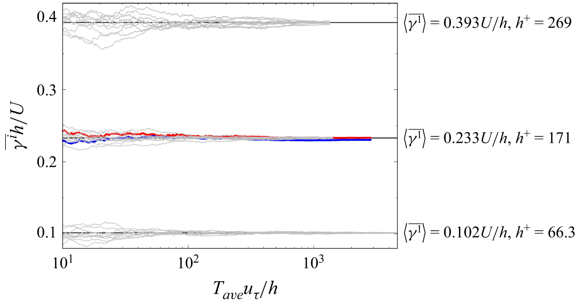
 (L1,L3)=(2πh,πh)
 Taveuτ/h
 ⟨γ1¯⟩h/U=0.102,0.233,
 h+=66.3,171
 h+=171
 γ1¯=0.233U/h
 γ2¯=0.230U/h
 Taveuτ/h=2840
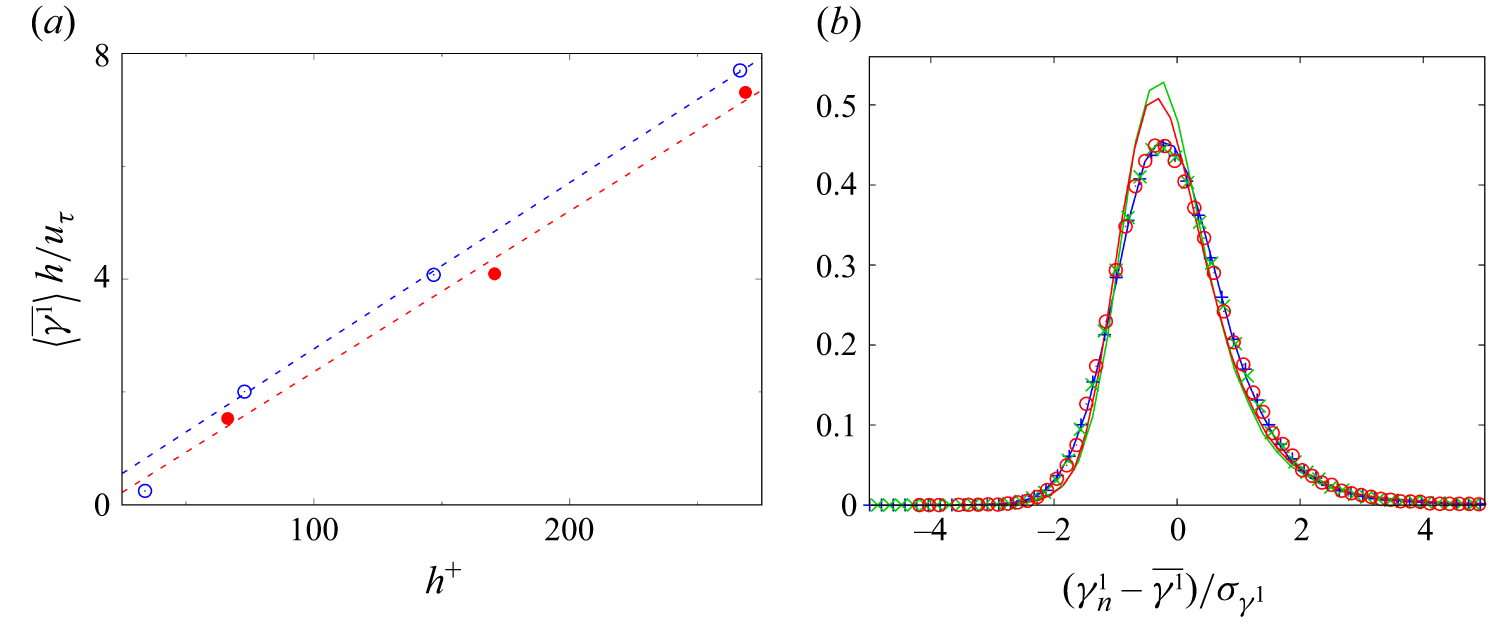
 (L1,L3)=(2πh,πh)
 (h+,γ¯h/uτ)=(34.0,0.021)
 R=400
 (L1,L3)=(1.755πh,1.2πh)
 γ¯h/uτ∼0.0285h+
 (L1,L3)=(2πh,πh)
 γ¯h/uτ∼0.0295h+
 γn1
 σγ1
 (L1,L3)=(2πh,πh)
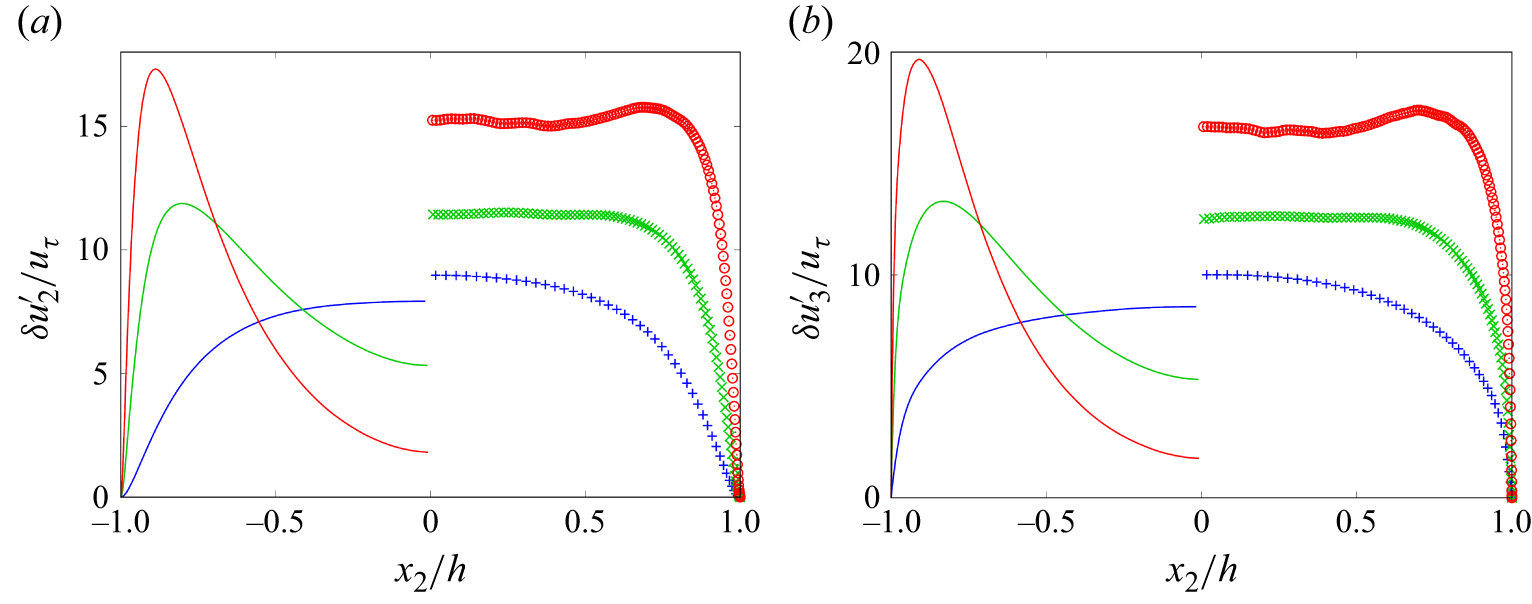
 δu2′/uτ
 δu3′/uτ
 (L1,L3)=(2πh,πh)
 (L1,L3)=(2πh,πh)

 h+=269
 k1E11
 k3E22
 y+=30.0
 y/h=0.65
 y=h−x2
 x2=h

 h+=269
 k1δE11
 k3δE22

 k1δE11
 k3δE22
 (L1,L3)=(2πh,πh)

 h+=171
 (L1,L3)=(2πh,πh)
 k1δE11
 k3δE22
 y+≃30.0
 y/h=1.00

 h+=269
 (L1,L3)=(2πh,πh)
 Qb=1.39×10³(uτ/h)2
 Qδξ1=1.39×10³(uτ/h)2
 0.333h/uτ

 h+=269
 (L1,L3)=(2πh,πh)

 [0,L1]×[−h,0]×[L3/2,L3]
 QL=13.9(uτ/h)2
 Qr=1.39×10³(uτ/h)2
 x2=−h
 x2=0


 δu1
 δu2
 y+=30
 (x2+=−239)
 x3+=775
 δu1
 y+=30
 (x2+=−239)
 x1+=1370
 δu2

 h+=171
 (L1,L3)=(2πh,πh)
 δξn1
 δξn2
 δξn1
 δξn2′
 QL=1.55(uτ/h)2
 Qr=618(uτ/h)2
 δξn1
 δξn2
 Qδξ1=618(uτ/h)2
 Qδξ2=618(uτ/h)2
 δξn2′
 Qδξ2′=618(uτ/h)2

 ⟨δξn1,δξn2′⟩
 TU/h=1.0
 t+=203

 T=10
 δξn1
 δξn2
 δξn1
 δξn2′


