





1. Introduction
The exchange of scalars between complex terrain, such as vegetation canopies or urban areas, and the atmosphere is a critical environmental process. It governs a wide range of applications, including biosphere–atmosphere exchange, forest fires and the spread of pollution. Effective modelling of these scenarios requires a fundamental understanding of the turbulent transport mechanisms within the distinct flow layers near the surface. In this study, we define the canopy sublayer (CSL) as the region below the canopy height, which is characterised by high spatial variability in flow statistics and direct interaction with the canopy elements. Immediately above the canopy lies the roughness sublayer (RSL). The RSL is characterised by distinct features that differ from a classic boundary layer and is better represented by a mixing-layer analogy (Raupach et al. Reference Raupach, Finnigan and Brunet1996). Specifically, the RSL is defined by the dominance of sweep events over ejection events in momentum transport. Above the RSL lies the inertial sublayer (ISL), where the influence of individual roughness elements fades and the flow returns to a classic boundary layer structure that obeys the typical logarithmic velocity profile (Finnigan Reference Finnigan2000). It is worth noting that in cases involving tall forest canopies or complex topography, the existence of a distinct ISL is often questionable (Dias-Júnior et al. Reference Dias-Júnior2019; Mortarini et al. Reference Mortarini, Katul, Cava, Dias-Júnior, Dias, Manzi, Sörgel, Araújo and Chamecki2023).
A central challenge in modelling turbulent scalar exchange between canopies and the atmosphere is the inadequacy of eddy-diffusivity-based models (commonly referred to as
 $K$
-theory or gradient-diffusion models), which relate turbulent fluxes to local mean concentration gradients through a turbulent diffusion coefficient (Denmead & Bradley Reference Denmead and Bradley1985). This limitation has been attributed to several factors (Katul et al. Reference Katul, Cava, Siqueira and Poggi2013): (i) near-field effects associated with the source distribution; (ii) the imbalance between turbulent production and dissipation; and (iii) transport dominated by large, organised eddies with scales comparable to the canopy height. Banerjee et al. (Reference Banerjee, De Roo and Mauder2017) further demonstrated that this breakdown is closely related to the dynamics of coherent motions responsible for upward and downward scalar transport, emphasising their dominant role in the failure of the
 $K$
-theory within canopy flows.
This failure of
 $K$
-theory stands in stark contrast to scalar dispersion in canonical turbulent boundary layers (TBLs), where
 $K$
-theory has been shown to provide an adequate description of turbulent transport. In smooth-wall TBLs, numerous studies have shown that the turbulent scalar flux is well described by a local gradient-diffusion relationship. For example, Talluru et al. (Reference Talluru, Philip and Chauhan2018) showed that the sign of the turbulent scalar flux consistently corresponds to the negative of the mean concentration gradient and that the flux vanishes at the height of the mean-concentration peak, both of which are consistent with down-gradient transport and a positive turbulent diffusivity. Similarly, Lim & Vanderwel (Reference Lim and Vanderwel2023) reported that, although the turbulent diffusivity in a smooth-wall TBL is anisotropic and inhomogeneous, it remains positive at all heights. For elevated point sources over rough surfaces, both Fackrell & Robins (Reference Fackrell and Robins1982) and Iacobello et al. (Reference Iacobello, Marro, Ridolfi, Salizzoni and Scarsoglio2019) demonstrated a clear coincidence between the zero-crossing height of the scalar flux and the peak mean concentration. This correspondence ensures a positive turbulent diffusivity, supporting the use of
 $K$
-theory as an appropriate framework for scalar dispersion sufficiently far above the roughness elements, provided it is properly parametrised.
In contrast to the flow above the RSL or in canonical boundary layers, turbulent momentum transport within the RSL is dominated by intense sweep events. While defined as single-point temporal statistics, these events serve as the localised Eulerian signatures of the large-scale coherent motions governing canopy–atmosphere momentum exchange (Finnigan et al. Reference Finnigan, Shaw and Patton2009). Although the role of sweeps on momentum transfer is well established, their effect on scalar transport remains poorly understood. Most experimental studies of scalar dispersion above canopies have focused on sources distributed throughout the canopy (Katul et al. Reference Katul, Cava, Siqueira and Poggi2013). In these cases, wake interactions and local production obscure the underlying transport mechanisms (Raupach Reference Raupach1989). As a result, it remains challenging to disentangle the influence of large coherent motions within the RSL on the occurrence of counter-gradient scalar fluxes.
We hypothesise that the dominance of sweeps plays a crucial role in driving counter-gradient scalar transport in the RSL. In this paper, we test this hypothesis by quantifying the contribution of sweep events to the vertical scalar flux. Previous experimental studies (Legg et al. Reference Legg, Raupach and Coppin1986; Coppin et al. Reference Coppin, Raupach and Legg1986) and modelling efforts (Cassiani et al. Reference Cassiani, Radicchi and Albertson2007; Mortarini et al. Reference Mortarini, Franzese and Ferrero2009) have investigated the dispersion from single or multiple line sources near the canopy top. Because line sources inherently average out spanwise turbulent variations, they can mask the localised impact of coherent motions. To overcome this, the present study uses a point source located at the canopy top. By preventing lateral spatial averaging, this point-source configuration highlights the fully three-dimensional interaction between the scalar plume and individual sweep events. This allows us to directly observe how coherent RSL motions govern scalar exchange and identify the physical mechanisms responsible for the breakdown of classical gradient-diffusion models.
Our canopy model comprises elements at two different heights, representing a simplified version of vertical heterogeneity typical of natural vegetation. This set-up provides a physically meaningful intermediate regime between idealised uniform canopies and complex natural landscapes, and we studied various aspects of this model in the environmental wind tunnel in a series of previous works (Shig et al. Reference Shig, Babin, Shnapp, Fattal, Liberzon and Bohbot-Raviv2023; Shnapp et al. Reference Shnapp, Liberzon, Bohbot-Raviv and Fattal2024). Although the flow dynamics in the RSL immediately above the canopy are primarily governed by global scales rather than individual element variations (Raupach et al. Reference Raupach, Finnigan and Brunet1996), incorporating structural heterogeneity greatly enhances the environmental relevance of the study. We validated the flow field using detailed particle image velocimetry (PIV) and compared velocity statistics with those from the uniform-height ’tombstone’ canopy of Harman et al. (Reference Harman, Böhm, Finnigan and Hughes2016), which replicates the classic set-up of Raupach et al. (Reference Raupach, Coppin and Legg1986). These comparisons confirm that the flow above the canopy aligns with universal RSL scaling based on the top-layer density (Shig et al. Reference Shig, Babin, Shnapp, Fattal, Liberzon and Bohbot-Raviv2023). A summary of the flow field characterisation is provided in Appendix B.
The present study focuses on the vertical turbulent scalar fluxes. To contextualise our results, we refer to the pioneering canopy experiments of Legg et al. (Reference Legg, Raupach and Coppin1986), who investigated dispersion from an elevated line source. A direct quantitative comparison is precluded by the fundamental difference in source geometry (point versus line source). However, the underlying vertical trends are expected to be physically comparable. This is especially true regarding the behaviour of the turbulent diffusivity. Furthermore, to isolate transport features unique to the canopy environment, we qualitatively contrast our observations with the canonical point-source boundary-layer dispersion study by Fackrell & Robins (Reference Fackrell and Robins1982).
Beyond the mean transport and turbulent fluxes, characterising the statistical distribution of concentration fluctuations is essential for understanding elevated point-source dispersion (Cassiani et al. Reference Cassiani, Bertagni, Marro and Salizzoni2020). Unlike distributed or line sources, emissions from a localised point source generate a highly intermittent scalar field characterised by significant concentration fluctuations, particularly the source region (Fackrell & Robins Reference Fackrell and Robins1982). Accurately describing the concentration fluctuations requires modelling the probability density function (p.d.f.) of the scalar field. While analytical models, such as the
 $\varGamma$
-distribution, have been widely adopted to describe scalar fluctuations and higher-order moments (such as skewness and kurtosis) in various turbulent boundary layers (Nironi et al. Reference Nironi, Salizzoni, Marro, Mejean, Grosjean and Soulhac2015; Cassiani et al. Reference Cassiani, Bertagni, Marro and Salizzoni2020), their performance in canopy flows remains less explored (Cassiani et al. Reference Cassiani, Bertagni, Marro and Salizzoni2020; Papp et al. Reference Papp, Istók, Koren, Balczó and Kristóf2024). Specifically, it is unclear how the intense, sweep-dominated transport inherent to the RSL modifies the extreme-value tails of the concentration p.d.f. Therefore, examining these scalar statistics provides a necessary complement to the flux-based analysis.
This paper is organised as follows. Section 2 revisits the relevant theoretical background, including scalar flux budgets,
 $K$
-theory formulations, and the role of sweep and ejection events in scalar transport. Section 3 details the experimental set-up and data processing methods. The results are presented in § 4, beginning with an analysis of the independent velocity (§ 4.1) and concentration statistics (§ 4.2) to characterise the flow field and the scalar plume. We then analyse the simultaneous velocity-concentration statistics (§ 4.3) to test the validity of
 $K$
-theory and determine the role of coherent motions in the transport process. Finally, our findings and concluding remarks are presented in §§ 5 and 6, respectively.
2. Theoretical framework
This section presents a theoretical framework for analysing turbulent scalar transport. It begins with the fundamental advection–diffusion equation and progresses to higher-order statistical models that connect the failure of
 $K$
-theory to the dynamics of coherent turbulent motions. Because this study focuses on neutrally stable conditions, buoyancy-related terms involving temperature fluctuations vanish and are therefore omitted, and the fluid density is assumed to be constant.
The transport of a passive scalar concentration,
 $c$
, within a turbulent flow field is governed by the advection–diffusion equation. Applying a Reynolds decomposition and averaging scheme to all variables (
 $c = \overline {c} + c'$
) separates an instantaneous concentration
 $c$
into a time-averaged mean
 $\overline {c}$
and a fluctuating
 $c'$
component, which yields the transport equation for the mean scalar concentration,
 $\overline {c}$
:
 \begin{align} \frac {\partial \overline {c}}{\partial t} + \overline {\boldsymbol{u}} \boldsymbol{\cdot }\boldsymbol{\nabla }\overline {c} = D \boldsymbol{\nabla} ^2 \overline {c} - \boldsymbol{\nabla }\boldsymbol{\cdot }\overline {\boldsymbol{u}' c'}. \end{align}
In (2.1),
 $\overline {\boldsymbol{u}}$
denotes the mean velocity vector and
 $D$
is the molecular diffusivity. The source term is omitted as it is zero everywhere except at the localised scalar source,
 $x=0$
. In this study,
 $x$
,
 $y$
and
 $z$
denote the streamwise, spanwise and wall-normal coordinates, respectively, and
 $u$
,
 $v$
and
 $w$
represent the corresponding velocity components. The coordinate origin is located at the wall, vertically aligned with the source outlet (see figure 1).
Focusing on the region above the canopy, the mean vertical and spanwise velocities are negligible (
 $\overline {w} \approx \overline {v} \approx 0$
). By further neglecting molecular diffusion, (2.1) simplifies to the following balance (Stull Reference Stull2012):
 \begin{align} \overline {u} \frac {\partial \overline {c}}{\partial x} = - \frac {\partial \overline {u'c'}}{\partial x} - \frac {\partial \overline {w'c'}}{\partial z} - \frac {\partial \overline {v'c'}}{\partial y}. \end{align}
Although the streamwise turbulent flux (
 $\overline {u'c'}$
) is of the same order of magnitude as the vertical turbulent flux (
 $\overline {w'c'}$
), it is dynamically negligible compared with the mean streamwise advection (
 $\overline {u}\,\overline {c} \gg \overline {u'c'}$
) (Stull Reference Stull2012). Assuming a horizontally homogeneous mean flow (
 $\partial \overline {u}/\partial x \approx 0$
), the total streamwise transport simplifies as
 $({\partial }/{\partial x}) (\overline {u}\,\overline {c} + \overline {u'c'}) \approx ({\partial }/{\partial x}) (\overline {u}\,\overline {c}) \approx \overline {u} ({\partial \overline {c}}/{\partial x})$
. Consequently, the turbulent scalar flux term in (2.1),
 $-\boldsymbol{\nabla }\boldsymbol{\cdot }(\overline {\boldsymbol{u}' c'})$
, reduces to its transverse components, which govern the spanwise and vertical dispersion of the plume (Stull Reference Stull2012). Given that this study primarily investigates vertical exchange, our analysis focuses specifically on the vertical scalar transport term,
 $\overline {w'c'}$
.
Equations (2.1) and (2.2) cannot be solved for unknowns
 $\overline {c}$
,
 $\boldsymbol{u}$
and
 $\overline {\boldsymbol{u}' c'}$
relying solely on the conservation of mass and momentum. One common approach to addressing the problem is to treat turbulence as a diffusive process and model the turbulent scalar flux
 $\overline {\boldsymbol{u}' c'}$
using a first-order gradient transport model analogous to Fick’s law, known as
 $K$
-theory (Csanady Reference Csanady1973). In this formulation, the vertical scalar transport is estimated as
 \begin{align} \overline {w'c'} = -D_{t} \frac {\partial \overline {c}}{\partial z}, \end{align}
where
 $D_{t}$
is the turbulent diffusivity in the
 $z$
(vertical) direction. This approximation assumes that the turbulent scalar flux is proportional to the mean scalar concentration gradient. Equation (2.3) is analogous to Boussinesq’s turbulent viscosity model for Reynolds stresses (Stull Reference Stull2012):
 \begin{align} \overline {u' w'} = -\nu _t \frac {\partial \overline {u}}{\partial z}, \end{align}
where
 $\overline {u'w'}$
represents the turbulent shear stress and
 $\nu _t$
is the so-called ‘turbulent viscosity’.
A common way to express turbulent diffusivity is through the turbulent Schmidt number,
 $Sc_t$
, defined as the ratio of turbulent viscosity (
 $\nu _t$
) to turbulent diffusivity (
 $D_t$
). It represents the relative efficiency of turbulent momentum transport compared with that of mass (Stull Reference Stull2012):
 \begin{align} D_t = \frac {\nu _t}{Sc_t} .\end{align}
This allows us to relate the turbulent scalar flux to the turbulent momentum flux, which is often easier to measure and model.
The
 $K$
-theory assumption of (2.3) works only if the turbulence transport length scale is much shorter than the scale at which the mean concentration field changes (Corrsin Reference Corrsin1975). In the RSL and near the canopy top, vertical turbulent transport is governed by organised motion whose scale is comparable to the canopy height (Finnigan Reference Finnigan2000). Thus, transport may be governed by large-scale motions linked to the failure of
 $K$
-theory (Banerjee et al. Reference Banerjee, De Roo and Mauder2017).
In regions exhibiting counter-gradient transport, Deardorff (Reference Deardorff1972) proposed to modify the usually applied flux-gradient relationship in the
 $K$
-theory approach according to
 \begin{align} \overline {w'c'} = -D_t \left ( \frac {\partial \overline {c}}{\partial z} + \varPi _c \right ), \end{align}
where
 $D_t\varPi _c$
represents the non-local flux term.
 $K$
-theory connects the local turbulent flux to the local mean gradient. Thus,
 $D_t\varPi _c$
captures the deviations from
 $K$
-theory, accounting for non-local fluxes and particularly counter-gradient transport. In this context, we define non-local transport as scalar exchange mechanisms that are decoupled from the local mean concentration gradient. In the literature, this transport is typically associated with large-scale structures and often leads to counter-gradient fluxes (Ghannam et al. Reference Ghannam, Duman, Salesky, Chamecki and Katul2017; Heisel et al. Reference Heisel, Katul, Chamecki and Guala2020).
To further estimate the non-local transport, we use the vertical flux budget neglecting the pressure diffusion term and molecular diffusion. Considering the region of the RSL above the canopy along the plume symmetry plane, the budget reduces to (Stull Reference Stull2012)
 \begin{align} \overline {u}\frac {\partial \overline {w'c'}}{\partial x} = -\overline {w'w'}\frac {\partial \overline {c}}{\partial z} -\overline {u'w'}\frac {\partial \overline {c}}{\partial x} -\frac {\partial \overline {w'w'c'}}{\partial z} -\frac {\partial \overline {v'w'c'}}{\partial y} -\frac {\partial \overline {u'w'c'}}{\partial x} -\frac {1}{\rho }\overline {c'\frac {\partial p'}{\partial z}}. \end{align}
The term on the left-hand side is the advection of
 $\overline {w'c'}$
by the mean flow. The terms on the right-hand side of the equation are respectively production by gradients in mean concentration, transport by turbulent-velocity fluctuations and pressure–concentration-gradient correlation.
At a certain distance from the source, along the source symmetry plane (
 $y/h=0$
), the budget equation can be simplified into an idealised far-field limit. This is achieved by assuming that streamwise and spanwise gradients are negligible compared with vertical gradients, an assumption justified only for the flow field above the canopy, where the spatial variability of flow statistics diminishes. Under these conditions, the equation reduces to
 \begin{align} 0 = -\overline {w'w'}\frac {\partial \overline {c}}{\partial z} -\frac {\partial \overline {w'w'c'}}{\partial z} -\frac {1}{\rho }\overline {c'\frac {\partial p'}{\partial z}}. \end{align}
However, within the CSL and to some extent above it, the spatial heterogeneity of the mean flow and turbulent fluxes introduces additional terms to this balance. Therefore, while (2.8) serves as a theoretical framework to isolate the role of the vertical triple correlation, its application to experimental data must be approached with caution.
The final term on the right-hand side of (2.8) represents the pressure-scalar gradient interaction, which acts as a decorrelation mechanism. Following the classic ‘return-to-isotropy’ concept originally proposed by Rotta (Reference Rotta1951) for the pressure–velocity gradient covariance in turbulent shear flows, numerous studies have extended this framework to model the pressure–concentration-gradient correlation term (Cava et al. Reference Cava, Katul, Scrimieri, Poggi, Cescatti and Giostra2006; Ghannam et al. Reference Ghannam, Duman, Salesky, Chamecki and Katul2017):
 \begin{align} \frac {1}{\rho }\overline {c'\frac {\partial p'}{\partial z}} = \frac {C_1}{\tau _R} \overline {w'c'}+C_2\overline {w'w'}\frac {\partial \overline {c}}{\partial z}, \end{align}
where
 $\tau _R$
is a relaxation time scale, and
 $C_1$
and
 $C_2$
are closure constants analogous to the Rotta constant and the isotropisation constant, respectively (Cava et al. Reference Cava, Katul, Scrimieri, Poggi, Cescatti and Giostra2006; Ghannam et al. Reference Ghannam, Duman, Salesky, Chamecki and Katul2017).
Substituting (2.9) into (2.8) we can show that
 \begin{align} \overline {w'c'} = -\frac {\tau _R}{C_1}\bigg ((1+C_2)\overline {w'w'}\frac {\partial \overline {c}}{\partial z}+\frac {\partial \overline {w'w'c'}}{\partial z}\bigg ). \end{align}
It is noteworthy that in flows where the vertical turbulent transport of flux is negligible, (2.10) is equivalent to the gradient-diffusion formulation (2.3). Hence, the failure of the
 $K$
-theory is associated with the non-negligible triple moments. The non-local flux term in (2.6) is therefore proportional to the vertical flux transport term:
 \begin{align} \varPi _c = C_3 \frac {\partial \overline {w'w'c'}}{\partial z}, \end{align}
where
 $C_3$
is the proportionality constant relating the non-local flux to the vertical flux transport.
Previous studies have demonstrated the strong connection between the sweep-ejection motions and the triple moments (Katul et al. Reference Katul, Hsieh, Kuhn, Ellsworth and Nie1997; Heisel et al. Reference Heisel, Katul, Chamecki and Guala2020). Therefore, we highlight the connection between sweep dominance at the RSL and the failure of the gradient diffusion assumption.
2.1. Quadrant analysis
Quadrant analysis is a widely used technique for examining coherent motions in turbulent shear flows by decomposing the Reynolds stress (Wallace Reference Wallace2016). The method partitions the
 $u'{-}w'$
plane into four quadrants (
 $Q_k$
,
 $k=1{-}4$
) according to the signs of the fluctuating velocity components: outward interactions (
 $Q_1$
:
 $u'\gt 0, w'\gt 0$
), ejections (
 $Q_2$
:
 $u'\lt 0, w'\gt 0$
), inward interactions (
 $Q_3$
:
 $u'\lt 0, w'\lt 0$
) and sweeps (
 $Q_4$
:
 $u'\gt 0, w'\lt 0$
), respectively.
The relative contribution of each quadrant
 $Q_k$
to the statistical moment of any order (
 $l+ m + n$
)
 $\overline {\hat {u}^l \hat {w}^m \hat {c}^n}$
is given by
 \begin{align} \overline {\hat {u}^l \hat {w}^m \hat {c}^n}_{k} = s_{u,k}^l s_{w,k}^m \int _{-\infty }^{\infty } \int _{0}^{\infty } \int _{0}^{\infty } \hat {u}^l \hat {w}^m \hat {c}^n P(s_{u,k}\hat {u}, s_{w,k}\hat {w}, \hat {c}) \ \text{d}\hat {u}\ \text{d}\hat {w}\ \text{d}\hat {c}, \end{align}
where the circumflex denotes a fluctuation normalised by its corresponding root-mean-square (r.m.s.) value,
 $\hat {\phi } = \phi ' / \sigma _{\phi }$
, with
 $\sigma _{\phi } = (\overline {{\phi '}^2})^{1/2}$
. The sign functions
 $s_{u,k} = (1, -1, -1, 1)$
and
 $s_{w,k} = (1, 1, -1, -1)$
specify the signs of
 $u'$
and
 $w'$
defining each quadrant
 $Q_k$
, where
 $k \in \{1, 2, 3, 4\}$
. These sign functions enforce the quadrant constraints, allowing conditional moments to be expressed as integrals over a fixed positive domain
 $[0, \infty )$
. Here,
 $P$
denotes the joint p.d.f. of normalised velocity and concentration fluctuations. According to these definitions, the sum of all quadrant contributions yields the total moment:
 $\sum _{k=1}^4 \overline {\hat {u}^l \hat {w}^m \hat {c}^n}_{k}=\overline {\hat {u}^l \hat {w}^m \hat {c}^n}$
.
Events in the second and fourth quadrants (
 $Q_2$
: ejections,
 $Q_4$
: sweeps) are the dominant contributors to the Reynolds stress (Finnigan Reference Finnigan2000). For momentum, the mean velocity gradient is positive at all heights (
 $\partial \overline {u}/\partial z\gt 0$
), because the canopy acts as a momentum sink and the free stream turbulent flow above the canopy acts as the momentum source. Therefore, both sweeps and ejections contribute negative values to the total momentum flux (
 $\overline {u'w'}_2\lt 0$
and
 $\overline {u'w'}_4\lt 0$
). These events produce strictly down-gradient momentum transport, transferring high-momentum fluid downward and low-momentum fluid upward, consistent with the gradient-diffusion relation (2.4). As established in the literature, particularly in the context of canopy flows, these events have been linked to large-scale coherent motions that exhibit both spatial and temporal correlation (Finnigan Reference Finnigan2000; Finnigan et al. Reference Finnigan, Shaw and Patton2009). Therefore, while the quadrant events in this study are defined strictly via single-point temporal statistics, they serve as localised Eulerian signatures of the large-scale coherent motions driving this transport (Brunet Reference Brunet2020).
Crucially, while sweeps and ejections are fundamentally down-gradient momentum transport mechanisms, this is not necessarily true for their contribution to scalar transport. Their specific role in vertical scalar exchange depends heavily on the mean scalar field. The mean concentration profile of a scalar released from an elevated localised source,
 $\overline {c}(z)$
, typically exhibits a maximum, such that the mean gradient
 $\partial \overline {c}/\partial z$
is positive below the maximum and negative above it. Therefore, a single momentum-defined quadrant event may represent the transport of a scalar either down or against the local mean gradient, depending entirely on the sign of the scalar fluctuation it carries.
To quantify the contribution of sweeps and ejections to the vertical scalar flux, we conditionally sample
 $w'c'$
using the momentum-based quadrants (
 $u'{-}w'$
), following the approach of Nagano & Tagawa (Reference Nagano and Tagawa1988). For example, a sweep event (
 $u'\gt 0, w'\lt 0$
) can contribute either positively or negatively to the vertical scalar flux
 $\overline {w'c'}$
, as illustrated in figure 1. If a sweep entrains fluid that is cleaner than the concentration average (
 $c'\lt 0$
), it produces a positive scalar flux contribution (
 $\overline {w'c'}_4\gt 0$
). We classify this as a ‘clean sweep’. If a clean sweep occurs in a region where
 $\partial \overline {c}/\partial z\gt 0$
(such as below a canopy-top source), it results in the counter-gradient transport contribution, thus leading to an apparently negative turbulent eddy diffusivity and ‘breaking’ the K-theory assumptions. Conversely, a ‘contaminated sweep’ entrains fluid with a higher-than-average concentration (
 $c'\gt 0$
), resulting in a negative scalar flux (
 $\overline {w'c'}_4\lt 0$
). The classification is applied similarly to ejections and summarised in table 1, showing that there are two types of ‘clean’ events and two types of ‘contaminated’ events, contributing differently to the scalar vertical transport term.
Interpretation of sweep and ejection scalar content (clean or contaminated) derived from the sign of the vertical scalar flux (
 $w'c'$
).

Table 1. Long description
A table summarizing the classification of sweep and ejection events based on their contribution to vertical scalar flux. The table has two rows and five columns. Column headers are Event, Sweep, Ejection, Clean Event, and Contaminated Event. Row 1: Event, Sweep, Ejection, Clean Event, Contaminated Event. Row 2: Sweep, Ejection, Clean Event, Contaminated Event.
Illustration of quadrant events, and their contribution to vertical momentum and scalar flux. The right side illustrates the resulting instantaneous scalar flux sign (
 $w'c'$
) for ’contaminated’ (
 $c' \gt 0$
) and ’clean’ (
 $c' \lt 0$
) fluid parcels. Arrows indicate the vertical velocity direction.

Conditioning the scalar flux using momentum-defined quadrants provides a direct means of identifying the coherent motions responsible for counter-gradient scalar transport. It is worth noting that an alternative methodological choice in the study of coherent motions and scalar flux is to apply quadrant analysis directly to the scalar flux plane (
 $w'{-}c'$
), as done in several canopy studies (Li & Bou-Zeid Reference Li and Bou-Zeid2011; Huang et al. Reference Huang, Katul and Albertson2013). While this direct scalar approach has distinct advantages for investigating metrics such as transport efficiency and requires only two variables, it presents a significant limitation for the specific aims of the present study. Defining quadrants in the
 $w'{-}c'$
plane makes the resulting event definitions depend entirely on the local scalar flux. In flows where the mean scalar gradient changes sign with height, such as above and below an elevated source, the very definitions of scalar sweeps and ejections in the
 $w'{-}c'$
plane become height-dependent. Another issue is that a scalar-defined sweep does not necessarily correspond to a momentum-defined sweep (
 $u'\gt 0, w'\lt 0$
). This makes it difficult to establish a direct relationship between the dominant, turbulent kinetic energy-producing motions and their specific role in scalar transport. Our momentum-based methodology avoids this ambiguity, providing a clear advantage by directly coupling the scalar fluxes to the driving flow dynamics.
2.2. Connecting the sweep-ejection balance to the triple moments
As demonstrated by (2.11), the triple moment is the leading contribution to a non-local scalar flux. Using the statistical framework of Nagano & Tagawa (Reference Nagano and Tagawa1988), we establish an analytical connection between the triple moment and the relative scalar flux contributions of sweep and ejection events (A4). This framework employs a three-variable joint p.d.f. expansion with cumulants and one-dimensional Hermite polynomials up to the fourth order (Nagano & Tagawa Reference Nagano and Tagawa1988). The complete derivation, including all expansion coefficients and integration steps, is provided in Appendix A.
The so-called Reynolds stress fraction, derived based on momentum quadrant analysis,
 $\Delta S_{uw}$
, quantifies the relative imbalance between sweep and ejection contributions to the momentum flux:
 \begin{align} \Delta S_{uw} = \frac {\overline {u'w'}_4-\overline {u'w'}_2}{\overline {u'w'}} = \frac {\overline {\hat {u}^2\hat {w}}-\overline {\hat {u}\hat {w}^2}}{2\sqrt {2\pi }\ \overline {\hat {u}\hat {w}}}. \end{align}
Similarly, we define the scalar flux fraction,
 $\Delta S_{wc}$
, as the sweeps and ejections contribution imbalance to the vertical scalar flux and is defined as:
 \begin{align} \Delta S_{wc} = \frac {\overline {w'c'}_4-\overline {w'c'}_2}{\overline {w'c'}} = \frac {\overline {\hat {u}\hat {w}\hat {c}}-3\overline {\hat {w}^2\hat {c}}}{12\sqrt {\pi /2}\ \overline {\hat {w}\hat {c}}}. \end{align}
It has been shown that there is a proportionality between the mixed moments measured at RSL (Katul et al. Reference Katul, Hsieh, Kuhn, Ellsworth and Nie1997). Thus, assuming
 $\overline {\hat {u}\hat {w}\hat {c}}= \alpha \ \overline {\hat {w}^2\hat {c}}$
, we can rewrite (2.14) as
 \begin{align} \overline {w'w'c'} = \frac {12\sqrt {\pi /2}}{\alpha -3}\sigma _w\overline {w'c'}\Delta S_{wc}. \end{align}
Thus, (2.15) establishes a direct link between the sweep-ejection imbalance (
 $\Delta S_{wc}$
) and the flux transport term (
 $\overline {w'w'c'}$
). As shown in (2.11), this flux transport term may represent the mechanism responsible for driving the non-local flux term
 $\varPi _c$
. This connection offers a valuable diagnostic framework: the measurable imbalance between sweeps and ejections can be used to infer the presence and magnitude of non-local transport, an effect that underlies the breakdown of
 $K$
-theory in scalar transport.
We note that previous studies have also analytically linked the flux-transport term,
 $\overline {w'w'c'}$
, to the relative contributions of sweep and ejection events (Cava et al. Reference Cava, Katul, Scrimieri, Poggi, Cescatti and Giostra2006; Banerjee et al. Reference Banerjee, De Roo and Mauder2017; Ghannam et al. Reference Ghannam, Duman, Salesky, Chamecki and Katul2017). However, those approaches relied solely on a two-variable joint p.d.f. restricted to the
 $w'{-}c'$
plane. In addition, their conditional quadrant analysis was based on the scalar flux plane, which, as stated already, fundamentally changes the definition of sweeps and ejections.
Schematics of the experimental set-up shown in side and top views: (a) cross-section of the tunnel working section; (b) top view showing the layout of roughness elements forming the canopy. The red and blue shaded rectangles represent two unit-cells, referred to as the ‘near-cell’ and ‘far-cell,’ respectively, where measurements were conducted. Crosses noted by either N or F indicate specific measurement locations. The red line in panel (a) and the red point in panel (b) mark the position of the ethane source. The canopy height is
 $h=100$
mm.

Figure 2. Long description
Panel A: A side view cross-section of the tunnel working section. The diagram includes spires, an ethane source, and measurement points. The canopy height is marked as h. The measurement point is indicated with FFID and LDV. The ethane source is marked with a red line. Panel B: A top view showing the layout of roughness elements forming the canopy. The red and blue shaded rectangles represent two unit-cells, referred to as the near-cell and far-cell, respectively, where measurements were conducted. Crosses noted by either N or F indicate specific measurement locations. The red point marks the position of the ethane source.
3. Methodology and experimental set-up
The experiments were conducted in the low-velocity boundary-layer wind tunnel at the Israel Institute for Biological Research (IIBR) under neutrally stratified conditions. The two-height canopy set-up is nearly identical to that described in our previous work, where we characterised the flow field using PIV (Shig et al. Reference Shig, Babin, Shnapp, Fattal, Liberzon and Bohbot-Raviv2023). In the current point-source dispersion study, the only modification was an increase in the streamwise extent of the canopy array. A schematic description of the experimental set-up is shown in figure 2(a). Simultaneous measurements of velocity and concentration were obtained using 2-component laser Doppler velocimetry (LDV) and a fast flame ionisation detector (FFID), respectively.
Full details of the wind tunnel facility are provided by Shig et al. (Reference Shig, Babin, Shnapp, Fattal, Liberzon and Bohbot-Raviv2023) and are briefly reviewed here. The test section is
 $15$
m long with a uniform cross-section of
 $2 \times 2$
m
 $^2$
. The canopy model was placed on the floor of the test section, spanning an area of approximately
 $11 \times 2$
m
 $^2$
, as shown schematically in figure 2(a). For the present study, the free stream velocity was set to
 $U_e=9.5$
m s
 $^{-1}$
, resulting in a bulk Reynolds number of
 $ \textit{Re}=5.3\times 10^5$
. Here, the bulk Reynolds number is defined as
 $ \textit{Re}=\delta U_e/\nu$
, where
 $\delta$
is the boundary-layer thickness at the measurement location and
 $\nu =1.5\times 10^{-5}$
m
 $^2$
s
 $^{-1}$
is the kinematic viscosity of air. The boundary-layer thickness,
 $\delta$
, is defined as the height at which a fitted power-law velocity profile reaches
 $U_e$
. The streamwise pressure gradient within the test section is negligible under these flow conditions. Additional boundary-layer parameters are summarised in table 2.
Flow properties and canopy parameters for the experimental boundary layer set-up.

Table 2. Long description
The table compares flow properties and canopy parameters for three different experimental set-ups: TH-canopy, HA16, and NE08-C. It has 10 rows and 4 columns. The columns are labeled Parameter, TH-canopy, HA16, and NE08-C. The rows list various parameters such as Canopy name, Reference, Layout pattern, Canopy height h (mm), Relative depth δ/h, Frontal area index λ, Friction velocity u*/Uh, Shear length scale Ls/h, Zero-plane displacement d/h, and Reynolds number Reh. Each row provides specific values for each parameter across the three set-ups. For example, the Canopy height h (mm) for TH-canopy is 100, for HA16 is 60, and for NE08-C is 50. The table provides a detailed comparison of these parameters across the different set-ups.
The friction velocity,
 $u_*$
, was estimated as the square root of the mean Reynolds shear stress evaluated at the canopy height (Shig et al. Reference Shig, Babin, Shnapp, Fattal, Liberzon and Bohbot-Raviv2023). Additionally, the flow is characterised by the ratio
 $u_*/u_h$
(where
 $u_h$
is the mean velocity at the canopy top), which serves as a measure of canopy turbulence. Both velocity scales were derived from the spatially averaged LDV profiles. These spatial averages were validated against the detailed PIV campaign from Shig et al. (Reference Shig, Babin, Shnapp, Fattal, Liberzon and Bohbot-Raviv2023), demonstrating excellent agreement with the present LDV measurements (see Appendix B for the complete comparison).
As noted in § 2, we denote
 $x$
,
 $y$
and
 $z$
as the streamwise, spanwise and floor-normal coordinates (figure 2
a). The origin of the axis is at the wall in correspondence to the source outlet location (figure 2
b).
The canopy is made of vertical thin metal plates of two heights,
 $100$
and
 $50$
mm, with a width of
 $50$
mm, arranged on the tunnel’s floor with their large faces perpendicular to the streamwise direction. Each spanwise row of elements consists of either tall or short elements in a staggered arrangement, resulting in an alternating tall–short pattern along the main flow direction (figure 2
b). The tall elements denote the term ‘canopy height’,
 $h$
(
 $=100$
mm). The canopy spreads the tunnel width and extends
 $110 h$
along the streamwise direction starting right after a set of spires at the tunnel’s inlet (figure 2
a). Four spires were placed upstream of the roughness elements to simulate a typical rough boundary layer, as shown schematically in figure 2(a). The total frontal area index,
 $\lambda$
, defined as the total projected facade area of the roughness elements per total horizontal wall area, was
 $\lambda = 0.5$
. The distribution of element heights results in a height-dependent frontal area index, which is at the bottom twice that of the top,
 $\lambda _{\textit{bottom}} = 2\lambda _{\textit{top}} = 1/3$
, as detailed by Shig et al. (Reference Shig, Babin, Shnapp, Fattal, Liberzon and Bohbot-Raviv2023). Consistent with existing literature, this frontal area density is sufficient to induce a mixing-layer-like flow regime, distinguishing it from a typical boundary-layer flow (Brunet Reference Brunet2020). For a detailed aerodynamic characterisation and comparison of the flow statistics with uniform-height canopies (e.g. Nezu & Sanjou Reference Nezu and Sanjou2008; Harman et al. Reference Harman, Böhm, Finnigan and Hughes2016), the reader is referred to Appendix B.
Streamwise (
 $u$
) and vertical (
 $w$
) velocity components were measured using a two-component LDV system (FiberFlow System, Dantec Dynamics, Denmark). The flow was seeded with glycerine-based aerosol droplets (particle size of approximately 1 μm) from a commercial Pea Soup smoke generator. Uniform seeding ensured high data acquisition rates, averaging approximately
 $250$
Hz within the canopy (
 $z/h\lt 1$
) and up to
 $600$
Hz above it (
 $z/h\gt 1$
). This spatial variation in data rate is characteristic of the LDV’s burst-mode operation, which depends on local particle concentration and velocity (Velte et al. Reference Velte, George and Buchhave2014).
The passive scalar was continuously released from an L-shaped tube located
 $90h$
downstream from the beginning of the canopy and at a height of
 $h_s \approx 0.95h$
. As shown in figure 2, the source is centred between two high elements, placing it at the canopy top near the region of maximum shear (Shig et al. Reference Shig, Babin, Shnapp, Fattal, Liberzon and Bohbot-Raviv2023). The tracer used was pure ethane (
 $\text{C}_2\text{H}_6$
), which is considered passive because its density is comparable to that of air. The source tube has an internal diameter of
 $d_s = 0.004$
m (
 $d_s/h \approx 0.04$
), and its flow rate was maintained between
 $1$
and
 $3$
litres per minute. To maintain a sufficient signal-to-noise ratio, higher rates were employed for measurements at downstream locations. We verified that this range of flow rates did not affect the normalised concentration statistics, thereby confirming that the plume behaved as a passive tracer.
The concentration,
 $c$
, was measured with a Combustion HFR400 FFID. The device was calibrated using certified calibration gases and was set to zero between runs by measurements without trace gas release. Concentration was measured in parts-per-million (ppm; molar fraction) and then normalised by a reference concentration indicating the source strength:
 \begin{align} c_s = \frac {\dot {m}_s}{h^2u_h}, \end{align}
where
 $\dot {m}_s$
is the source flow rate and
 $u_h$
is the mean velocity at the canopy top (
 $z/h=1$
).
The LDV and FFID probes were assembled together on a 3-axis traverse system, positioning the 0.25 mm FFID sampling tube in close proximity to the LDV measurement volume,
 $2$
mm downstream and
 $2$
mm above the LDV measurement volume, in accordance with the guidelines presented by Marro et al. (Reference Marro, Gamel, Méjean, Correia, Soulhac and Salizzoni2020). To estimate the correlation statistics between velocity and concentration, we set the acquisition system to trigger on LDV. Thus, the velocity and concentration signals are collected simultaneously when the seed particles cross the LDV sample volume. As a consequence, the concentration sampling rate is also irregular and exhibits the same bias as the LDV towards the faster-moving particles. As a result, each realisation was weighted by its residence time within the LDV sampling volume when calculating mean properties. Following George & Lumley (Reference George and Lumley1973), the mean value of any quantity, momen or correlation,
 $\phi$
, is explicitly calculated as follows:
 \begin{align} \overline {\phi }=\frac {\sum _{i=0}^N\phi _i \Delta t_{r,i}}{\sum _{i=0}^N\Delta t_{r,i}}. \end{align}
In this equation,
 $\phi _i$
represents the instantaneous value of the measured quantity due to the
 $i$
th particle and
 $\Delta t_{r,i}$
is the corresponding residence time of that particle within the LDV sampling volume.
The acquisition time was set to
 $T_s = 300$
seconds for each measurement point, ensuring sufficient statistical convergence for all measured quantities. Due to the length (
 $200$
mm) of the FFID sample tube, there is a small time delay between the sample taken and the gas analysis after travelling through the sampling tube. Therefore, similar to the work of Marro et al. (Reference Marro, Gamel, Méjean, Correia, Soulhac and Salizzoni2020), a time correction was applied. The corresponding time-shift value was calculated based on the device’s actual operating conditions. The mean delay in the physical sampling time relative to that of LDV was
 $15.6$
ms. Hence, all concentration signals are accordingly shifted and interpolated in time for analysis.
Measurements were taken at several locations marked by crosses in figure 2(b) within two distinct unit cells. These consisted of a near-cell (N) located
 $4.5h$
downstream of the source and a far-cell (F) at
 $10.5h$
downstream. Within each cell, four vertical profiles of simultaneous velocity-concentration data were acquired at specific locations: upstream and downstream of a tall element (
 $y/h=0$
), and upstream and downstream of a short element (
 $y/h=0.5$
). These locations are represented by the notation
 $N_{i,j}$
and
 $F_{i,j}$
, where
 $i (\in {1,2})$
denotes the streamwise position within the unit cell, and
 $j (\in {0.5,1})$
the position along the spanwise direction (crosses in the red and blue shaded squares in figure 2
b).
4. Results
This chapter presents the experimental results in two main parts. We first independently analyse the key statistical properties of the velocity and concentration signals at the denoted locations (figure 2). Following this, we assess the simultaneous velocity-scalar fluxes to examine the scalar vertical turbulent transport mechanisms.
4.1. Velocity statistics
The detailed turbulence statistics and flow structure for this specific canopy geometry were comprehensively analysed in our previous work using PIV (Shig et al. Reference Shig, Babin, Shnapp, Fattal, Liberzon and Bohbot-Raviv2023). Therefore, the primary objective of this section is not to repeat that characterisation, but strictly to present the specific local flow conditions at the measurement locations and determine the vertical extent of the RSL to contextualise the scalar transport analysis.
For completeness and validation, Appendix B provides a direct comparison between the current single-point LDV measurements and the independent PIV data. It also presents spatially averaged statistics, demonstrating that the flow exhibits canonical canopy turbulence characteristics similar to uniform-height canopy benchmarks (Nezu & Sanjou Reference Nezu and Sanjou2008; Harman et al. Reference Harman, Böhm, Finnigan and Hughes2016).
The flow at the measurement region is fully developed, supported by excellent agreement of velocity statistics between near (
 $N$
) and far (
 $F$
) canopy unit cells (see Appendix C). Figure 3 presents the vertical profiles of the normalised velocity statistics measured at individual locations within this cell, alongside the corresponding spatially averaged or double-averaged (DA) profiles.
The mean streamwise velocity profiles (figure 3
a) are characteristic of dense canopies, showing a displaced logarithmic profile above the canopy and an exponential profile shape in the canopy. The profile
 $F_{1,0}$
, taken downstream of a tall element, displays an inflection point with mean backflow near the canopy’s top, indicating a local mean recirculation zone sheltered by the tall element. The other three locations show nearly identical mean streamwise profiles below the canopy height (
 $z/h\lt 1$
). Above the canopy (
 $z/h\gt 1$
), all profiles converge into a nearly identical logarithmic profile. The variability observed within the canopy layer (
 $z/h\lt 1$
) is attributed to the local spatial heterogeneity inherent to single-point measurements.
Figures 3(b) and 3(c) show the r.m.s. profiles of the streamwise and vertical velocity fluctuations,
 $\sigma _u$
and
 $\sigma _w$
. The profiles at
 $F_{1,0}$
are distinctive. They exhibit the highest peaks near the canopy top and a sharp decline within the canopy itself. Conversely, the
 $F_{2,0}$
profile peaks within the canopy. Its streamwise velocity variance exceeds that of the profiles above the shorter elements at
 $F_{1,0.5}$
and
 $F_{2,0.5}$
. All variance profiles from the different locations converge above
 $z/h=1.2$
and remain nearly constant up to
 $z/h=3$
. In this upper region,
 $\sigma _u/u_*$
ranges from
 $1.7$
to
 $1.8$
. Similarly,
 $\sigma _w/u_*$
ranges from
 $1.1$
to
 $1.2$
. A comparison between the individual point measurements and the DA profiles reveals that for
 $z/h \gt 1.2$
, all profiles collapse onto the DA curve. This indicates that horizontal flow heterogeneity is negligible above this elevation and local point statistics accurately represent the spatially averaged flow field.
Vertical profiles of non-dimensional velocity statistics: (a) mean streamwise velocity; (b) r.m.s. streamwise velocity fluctuation (
 $\sigma _u$
); and (c) r.m.s. vertical velocity fluctuation (
 $\sigma _w$
). Coloured lines represent the local point profiles, whereas the black lines denote the DA profiles. The solid horizontal line indicates the canopy height (
 $z/h=1$
) and the dashed horizontal line marks the elevation (
 $z/h=1.2$
) above which horizontal heterogeneity becomes negligible and the point statistics collapse onto the DA curves.

Figure 3. Long description
Three line graphs depict vertical profiles of non-dimensional velocity statistics. Panel A shows the mean streamwise velocity, Panel B displays the root mean square (r.m.s.) streamwise velocity fluctuation, and Panel C illustrates the r.m.s. vertical velocity fluctuation. Each panel features multiple colored lines representing local point profiles and black lines denoting the DA profiles. The x-axes measure non-dimensional velocity values, while the y-axes indicate the height normalized by canopy height (z/h). A solid horizontal line marks the canopy height, and a dashed horizontal line indicates the elevation above which horizontal heterogeneity becomes negligible. The graphs show how velocity statistics vary with height and highlight the collapse of point statistics onto the DA curves above a certain elevation.
Figure 4 shows vertical profiles of the normalised turbulent shear stress (
 $\overline {u'w'}/u_*^2$
), turbulent viscosity (
 $\nu _t/hu_*$
) and stress fraction,
 $\Delta S_{uw}=(\overline {u'w'}_4-\overline {u'w'}_2)/\overline {u'w'}$
. The turbulent shear stress (figure 4
a) is negative at all measurement locations, with its magnitude peaking near the canopy top, as is typical for canopy flows. Above
 $z/h \gt 1.1$
, all profiles are nearly identical, while they diverge below this height. The profile downstream of the tall element,
 $F_{1,0}$
, exhibits the largest stress magnitude and the most rapid decay within the canopy.
The turbulent viscosity,
 $\nu _t=-\overline {u'w'}/(\partial \overline {u}/\partial z)$
(figure 4
b), varies significantly with height and location for
 $z/h \lt 1.2$
. Above this height, the local profiles converge and become approximately constant for
 $z/h \gt 2$
. Crucially, the strictly positive values of
 $\nu _t$
observed across all locations confirm that momentum is consistently transported down the mean velocity gradient. While the strong spatial variability below
 $z/h \lt 1.2$
precludes the definition of a simple local scalar viscosity, the consistently positive nature of these values indicates that a gradient-diffusion approach (
 $K$
-theory) remains a valid framework for modelling momentum transport within the RSL above the canopy, provided the parametrisation properly accounts for spatial heterogeneity.
The stress fraction,
 $\Delta S_{uw}$
(figure 4
c), provides insight into the turbulence structure. For
 $z/h \lt 1.8$
,
 $\Delta S_{uw}$
is positive, indicating that momentum transport is dominated by sweep events. This behaviour is characteristic of the RSL, where turbulence is strongly affected by the shear layer near the canopy top. Above the RSL (for
 $z/h \gt 2$
), the stress fraction approaches zero, signifying a balance between sweep and ejection motions and a transition towards an ISL. This implies that the region dynamically affected by the canopy extends well above the elements, consistent with the range
 $z/h \approx 2{-}3$
reported in the literature (Brunet Reference Brunet2020). Consequently, for the remainder of this study, we define the RSL upper boundary at
 $z/h=2$
, based on this turnover point.


Overall, the velocity statistics confirm that the flow exhibits the characteristic features of canopy turbulence. The region immediately surrounding the canopy top is characterised by an inflection point in the mean streamwise velocity profile, strong shear and momentum transport dominated by sweep events. At higher elevations, ejections become the dominant transport mechanism. This structural transition defines the upper limit of the RSL, which extends to
 $z/h \approx 2$
. It is important to note that while canopy flows are conventionally analysed using a DA framework, incorporating both spatial and temporal averaging, this section has examined temporally averaged point statistics at representative locations. By assessing the spatial variability among these individual profiles, we conclude that horizontal heterogeneity becomes negligible for
 $z/h \gt 1.2$
. Above this elevation, the local point statistics collapse onto the DA profiles, thus may be used to represent the DA statistics.
4.2. Concentration statistics
To characterise the dispersion process and assess how canopy-induced turbulence in the RSL influences scalar transport, we now turn to the statistical properties of the concentration field. We focus on the vertical distribution of the mean concentration, the intensity and intermittency of concentration fluctuations, and the higher-order moments describing the p.d.f. of the scalar field.
Figure 5 presents the vertical profiles of the mean concentration (
 $\overline {c}$
) and the r.m.s. of concentration fluctuations (
 $\sigma _c$
) along the source symmetry plane (
 $y/h=0$
) at the near (
 $N$
) and far (
 $F$
) canopy cells. To facilitate comparison across different streamwise positions, the profiles of both
 $\overline {c}$
and
 $\sigma _c$
are normalised by the respective local maximum of the mean concentration evaluated along each vertical measurement line. These maximum mean values, normalised by the reference source concentration (
 $c_s$
), are provided as
 $\overline {c}_{\textit{max}}/c_s$
in table 3.
Maximum normalised concentration (
 $c_{\textit{max}}/c_s$
) at the different measurement locations.

Table 3 Long description
The table presents maximum normalised concentration values at various measurement locations. It contains four columns and one row. The columns are labeled as follows: c_max/c_s, N_1,0, N_2,0, F_1,0, and F_2,0. The row provides the following values: 137.38, 118.52, 42.81, and 39.58.
As the scalar moves downstream, it rises and spreads vertically. The
 $\sigma _c$
profiles show the same upward shift and vertical broadening. However, at all downstream locations, the peak of
 $\sigma _c$
is located higher than the peak of the mean concentration height.
These trends are consistent with the findings of Fackrell & Robins (Reference Fackrell and Robins1982) for an elevated point source in a turbulent boundary layer, as well as with the point-source canopy dispersion study by Saeedi & Wang (Reference Saeedi and Wang2015). In contrast to the elevated line-source measurements of Legg et al. (Reference Legg, Raupach and Coppin1986), where the peak relative intensity,
 $\sigma _{c,\textit{max}}/\overline {c}_{\textit{max}}$
, drops below unity immediately downstream of the source, our point-source measurements maintain values greater than unity even in the far-field (
 $F$
) cells. This sustained intensity is physically expected: narrow point-source plumes are subject to lateral meandering, which generates significantly higher concentration fluctuations along the centreline compared with a statistically two-dimensional line source, which is horizontally homogeneous.
A notable feature emerges within the canopy (
 $z/h\lt 1$
), where the
 $\sigma _c$
values for the
 $N_{1,0}$
and
 $F_{1,0}$
profiles are smaller than those of their corresponding downstream profiles (
 $N_{2,0}$
and
 $F_{2,0}$
). This behaviour directly opposes the trend observed above the canopy (
 $z/h\gt 1$
), where fluctuations strictly decay with downstream distance. We attribute this localised decrease of concentration fluctuations to the sheltering effect of the canopy elements, a phenomenon that was also apparent in the velocity statistics presented in figure 3.
Vertical profiles along the source symmetry plane (
 $y/h=0$
) at different streamwise locations: (a) normalised mean concentration,
 $\overline {c}/\overline {c}_{\textit{max}}$
; (b) normalised r.m.s. concentration fluctuations,
 $\sigma _c/\overline {c}_{\textit{max}}$
. Corresponding
 $\overline {c}_{\textit{max}}/c_s$
values are provided in table 3.

Figure 5. Long description
Two line graphs depict vertical profiles along the source symmetry plane at different streamwise locations. Panel A: The line graph shows normalized mean concentration profiles. The vertical axis represents the normalized height (z/h) ranging from 0.5 to 4.0, and the horizontal axis represents the normalized mean concentration (c/c_max) ranging from 0 to 1.0. The graph includes four data series labeled N1,0, N2,0, F1,0, and F2,0, each represented by different colors and symbols. Panel B: The line graph shows normalized root mean square concentration fluctuations. The vertical axis represents the normalized height (z/h) ranging from 0.5 to 4.0, and the horizontal axis represents the normalized root mean square concentration fluctuations (σc/c_max) ranging from 0 to 2.0. The graph includes the same four data series labeled N1,0, N2,0, F1,0, and F2,0, each represented by different colors and symbols. Both graphs show how the concentration profiles and fluctuations vary with height and streamwise location.
Vertical profiles of (a) concentration intensity,
 $i_c$
, (b) peak concentration values,
 $c_{99}/\sigma _{c}$
, (c) concentration intermittency,
 $\gamma _c$
, and (d) concentration skewness,
 $M_{3c}$
. The black arrow in panel (a) indicates the decrease in intensity in the streamwise direction.

A key quantity for characterising the distribution of concentration fluctuations is the relative intensity, defined as
 $i_c=\sigma _c/\overline {c}$
. Figure 6(a) shows vertical profiles of
 $i_c$
at the different streamwise locations along the source symmetry plane (
 $y/h=0$
) and off-symmetry plane (
 $y/h=0.5$
). The most notable observation is that the relative intensity is substantially higher for the near-field profiles (
 $N_{1-2}$
) than for the far-field profiles (
 $F_{1-2}$
). Furthermore, the two sets of profiles exhibit distinct trends with height. In the far-field (
 $F_{1-2}$
), the intensity increases in a nearly linear fashion, rising from
 $i_c \approx 1$
at the canopy top to
 $i_c \approx 2$
at
 $z/h=3.5$
. In contrast, the near-field profiles (
 $N_{1-2}$
) show a similar linear trend only up to
 $z/h \approx 2.2$
, and transition to a steep, quasi-exponential rise, reaching values as high as
 $i_c \approx 5$
.
Two additional quantities used in characterising the concentration fluctuations are the peak concentration values and the scalar intermittency, presented in figures 6(b) and 6(c), respectively. For consistency with previous studies (e.g. Fackrell & Robins Reference Fackrell and Robins1982), the peak concentration is defined as the 99th percentile and normalised by the corresponding concentration fluctuations r.m.s. (
 $c_{99}/\sigma _c$
). Interestingly, the resulting normalised peak remains nearly constant throughout the entire plume, with a value of
 $c_{99}/\sigma _c \approx 4.6$
. This result agrees well with the findings of Fackrell & Robins (Reference Fackrell and Robins1982) for point-source dispersion in turbulent boundary layers.
The intermittency factor,
 $\gamma _c$
, is defined as the fraction of time the concentration signal is greater than a threshold value, that is, the probability that at a position
 $\boldsymbol{x}$
and time
 $t$
, the concentration
 $c$
is non-zero. To account for instrument limitations and uncertainty, a threshold,
 $\epsilon$
, is applied to the data before calculating
 $\gamma _c$
:
 \begin{align} c(x,y,z,t) = 0 \quad \text{if} \ c(x,y,z,t)\lt \epsilon, \end{align}
where
 $\epsilon =|\min [c(x,y,z,t)]|$
is the absolute value of the minimum amplitude of all concentration series.
The intermittency results are shown in figure 6(c). In both measured unit cells,
 $\gamma _c$
is highest within the canopy and decreases with height. As expected, the intermittency is higher in the far-field than in the near-field. In the far-field locations, the intermittency approaches unity (
 $\gamma _c \approx 1$
) within and just above the canopy. This observation, combined with the low relative intensity (
 $i_c \,\leq\, 1$
) in the same region, indicates that the plume is approaching the far-field state.
Given the high fluctuation intensity and peak values, it is useful to characterise the p.d.f. of concentration fluctuations. A key metric for this is the skewness, defined as
 $M_{3c}= \overline {\hat {c}^3}$
, with vertical profiles shown in figure 6(d). The profiles showcase distinct behaviours depending on the downstream location. In the far-field, the skewness is nearly constant above the canopy, maintaining a value of
 $M_{3c} \approx 3.5$
for
 $1 \,\leq\, z/h \,\leq\, 2$
. In contrast, the near-field profiles exhibit higher skewness that increases continuously with height, without a similar constant region. These trends are consistent for measurements on both the symmetry plane (
 $y/h=0$
) and off-symmetry plane (
 $y/h=0.5$
).
In the study of passive scalar dispersion, modelling the distribution of concentration fluctuations using analytical p.d.f.s provides a highly practical framework. Several such p.d.f. models have been evaluated over the years using wind-tunnel and field data (Cassiani et al. Reference Cassiani, Bertagni, Marro and Salizzoni2020). As a first step, we examine the consistency of our dataset with established functional dependencies between the moments of the concentration p.d.f. Chatwin & Sullivan (Reference Chatwin and Sullivan1990) developed a simple p.d.f. prediction model that neglects molecular diffusivity and assumes the scalar transport is dominated by large-scale motions. This model, which has been empirically verified for various shear flows (Cassiani et al. Reference Cassiani, Bertagni, Marro and Salizzoni2020), leads to specific relationships between concentration intensity (
 $i_c$
), skewness (
 $M_{3c}=\overline {\hat {c}^3}$
) and kurtosis (
 $M_{4c}=\overline {\hat {c}^4}$
):
 \begin{align} M_{3c} = a_1i_c+a_2i_c^{-1}, \\[-28pt] \nonumber \end{align}
 \begin{align} M_{4c} = b_1M_{3c}^{b_2}+b_3. \\[0pt] \nonumber \end{align}
Several p.d.f. models have been tested in the literature, including the clipped normal, Weibull and lognormal models. Among these, recent studies suggest that the
 $\varGamma$
-distribution is often a good approximation for the scalar concentration (Nironi et al. Reference Nironi, Salizzoni, Marro, Mejean, Grosjean and Soulhac2015; Cassiani et al. Reference Cassiani, Bertagni, Marro and Salizzoni2020).
 $\varGamma$
-distribution yields theoretical constants for (4.2) and (4.3) of
 $a_1=2$
,
 $a_2=0$
,
 $b_1=1.5$
,
 $b_2=2$
and
 $b_3=3$
. We tested this model by fitting these equations to our dataset (figure 7). In the figure, the dashed line represents the theoretical
 $\varGamma$
-distribution, while the solid line is the best fit to our data. This obtained fitted parameters are
 $a_1=2.6$
,
 $a_2=0.5$
,
 $b_1=2.6$
,
 $b_2=1.9$
and
 $b_3=3$
. The significant discrepancy between our fitted parameters and the theoretical values indicates that the
 $\varGamma$
-distribution underpredicts the skewness (
 $M_{3c}$
) and kurtosis (
 $M_{4c}$
) values for a given intensity.
(a) Skewness
 $M_{3c}$
against intensity
 $i_c$
, (b) Kurtosis
 $M_{4c}$
against skewness
 $M_{3c}$
. The relations
 $M_{3c} = a_1i_c+a_2i_c^{-1}$
and
 $M_{4c}= b_1M_{3c}^{b_2} + b_3$
are fitted to the data using least squares and shown as a black line; the corresponding
 $\varGamma$
-distribution relation is shown in a dashed black line.

Figure 7. Long description
Panel A: A scatter plot shows the relationship between skewness and intensity. The x-axis is labeled intensity with units, and the y-axis is labeled skewness with units. Different data sets are represented by colored circles: red for N1, green for N2, orange for F1, and blue for F2. A solid black line represents the fitted relation M3c = a1ic + a2ic^(-1), and a dashed black line represents the corresponding chi-distribution relation. Panel B: Another scatter plot shows the relationship between kurtosis and skewness. The x-axis is labeled skewness with units, and the y-axis is labeled kurtosis with units. The same color scheme is used for the data sets. A solid black line represents the fitted relation b1M3c^b2 + b3, and a dashed black line represents the corresponding chi-distribution relation.
To further evaluate the applicability of the
 $\varGamma$
-distribution, we examined the p.d.f. of the normalised concentration fluctuations,
 $c/\sigma _c$
. The theoretical curves were generated using a shape parameter determined locally by the fluctuation intensity,
 $k=i_c^{-2}$
, such that the first two moments of the model match the experimental data (Abramowitz & Stegun Reference Abramowitz and Stegun1965). Figure 8 presents the histograms of
 $c/\sigma _c$
at wall-normal heights
 $z/h=1.2$
,
 $1.6$
and
 $2.4$
across the four streamwise locations (
 $N_{1,0}$
,
 $N_{2,0}$
,
 $F_{1,0}$
and
 $F_{2,0}$
).
A comparison with the
 $\varGamma$
-curves reveals clear trends. While the model agrees well with the experimental data in the range
 $0.5\lt c/\sigma _c\lt 3$
, noticeable deviations occur at the distribution tails. Specifically, the
 $\varGamma$
-distribution overpredicts the probability of near-zero concentrations and underpredicts the frequency of extreme values. Because these extreme fluctuations strongly influence the higher-order moments (
 $M_{3c}$
and
 $M_{4c}$
), this mismatch explains the underprediction of skewness and kurtosis previously observed in figure 7.
Histograms of normalised concentration fluctuations,
 $c/\sigma _c$
, plotted on log–log scales with fitted
 $\varGamma$
-distributions (red lines). The panels are organised by wall-normal height (a:
 $z/h=2.4$
; b:
 $z/h=1.6$
; c:
 $z/h=1.2$
) and streamwise location (left to right:
 $N_{1,0}$
,
 $N_{2,0}$
,
 $F_{1,0}$
,
 $F_{2,0}$
).

4.3. Turbulent scalar flux
Direct measurements of turbulent scalar fluxes are crucial for understanding the physical mechanisms that govern turbulent scalar dispersion. The simultaneous LDV-FFID measurement technique provides valuable experimental data for which very limited prior measurements are available.
Figure 9 presents vertical profiles of the turbulent scalar flux,
 $\overline {w'c'}$
, together with the normalised mean scalar concentration at several downstream locations. The flux profile exhibits a distinct S-shape, a characteristic feature of elevated-source dispersion. The flux zero-crossing lies above the canopy and its height increases with downstream distance. The peak of the mean scalar concentration is likewise located above the canopy and rises as the plume moves downstream.
The central experimental finding is the misalignment between the zero-crossing of the turbulent flux (indicated by the dotted line) and the peak mean concentration. For elevated plumes in a classical turbulent boundary layer, these two vertical positions coincide (Fackrell & Robins Reference Fackrell and Robins1982; Talluru et al. Reference Talluru, Philip and Chauhan2018; Iacobello et al. Reference Iacobello, Marro, Ridolfi, Salizzoni and Scarsoglio2019). The observed separation, therefore, provides clear evidence of counter-gradient vertical scalar transport. Consequently, the assumptions underlying
 $K$
-theory are violated for this flow, a premise examined in detail in the following.
Vertical profiles of the turbulent scalar flux
 $\overline {w'c'}$
(black) and the normalised mean scalar concentration
 $\overline {c}/c_{max}$
(red) along the plume symmetry-plane. Panels (a)–(d) correspond to measurement locations
 $N_{1,0}$
,
 $N_{2,0}$
,
 $F_{1,0}$
and
 $F_{2,0}$
, respectively. The horizontal solid line denotes the canopy height
 $h$
, and the dotted line indicates the zero-crossing height of the vertical flux.

Figure 9. Long description
Panel A: A line graph shows vertical profiles of turbulent scalar flux in black and normalized mean scalar concentration in red. The x-axis represents the normalized vertical velocity fluctuation over friction velocity and maximum mean scalar concentration, ranging from 0 to 0.2. The y-axis represents the normalized height, ranging from 0.5 to 3. The solid horizontal line denotes the canopy height, and the dotted line indicates the zero-crossing height of the vertical flux. Panel B: A line graph shows vertical profiles of turbulent scalar flux in black and normalized mean scalar concentration in red. The x-axis represents the normalized vertical velocity fluctuation over friction velocity and maximum mean scalar concentration, ranging from 0 to 0.2. The y-axis represents the normalized height, ranging from 0.5 to 3. The solid horizontal line denotes the canopy height, and the dotted line indicates the zero-crossing height of the vertical flux. Panel C: A line graph shows vertical profiles of turbulent scalar flux in black and normalized mean scalar concentration in red. The x-axis represents the normalized vertical velocity fluctuation over friction velocity and maximum mean scalar concentration, ranging from 0 to 0.2. The y-axis represents the normalized height, ranging from 0.5 to 3. The solid horizontal line denotes the canopy height, and the dotted line indicates the zero-crossing height of the vertical flux. Panel D: A line graph shows vertical profiles of turbulent scalar flux in black and normalized mean scalar concentration in red. The x-axis represents the normalized vertical velocity fluctuation over friction velocity and maximum mean scalar concentration, ranging from 0 to 0.2. The y-axis represents the normalized height, ranging from 0.5 to 3. The solid horizontal line denotes the canopy height, and the dotted line indicates the zero-crossing height of the vertical flux.
4.4. Turbulent scalar diffusivity
Having characterised the turbulent scalar fluxes, we now assess the validity of
 $K$
-theory by evaluating the effective turbulent scalar diffusivity,
 $D_t$
, as defined in (2.3).
Figure 10 presents vertical profiles of the turbulent scalar diffusivity,
 $D_t=-(( {\overline {w'c'}})/({\partial \overline {c}/\partial z}))$
, at several streamwise locations. Profiles reveal distinct transport regimes across the vertical extent of the flow. The central finding of this study arises within the RSL (
 $1 \lt z/h \lt 2$
), indicated by the shaded area. In this region,
 $D_t$
exhibits substantial spatial scatter and, crucially, attains negative values. This effect is markedly more pronounced in the near (
 $N$
) cell than in the far (
 $F$
) cell. The negative diffusivity is non-physical, confirming the presence of counter-gradient scalar transport and the breakdown of
 $K$
-theory.
In contrast, above the RSL (
 $z/h \gt 2$
), the diffusivity becomes nearly constant with height, collapsing to a value of approximately
 $D_t/h u_* \approx 0.8$
across all measurement locations. Within the canopy (
 $z/h \lt 1$
),
 $D_t$
is significantly reduced and exhibits streamwise variability. The asymptotic behaviour above the canopy is in quantitative agreement with the elevated line-source experiments of Legg et al. (Reference Legg, Raupach and Coppin1986), which similarly reported a constant diffusivity for
 $z/h \gt 2$
. However, it is important to note that Legg et al. (Reference Legg, Raupach and Coppin1986) excluded data points yielding negative turbulent diffusivity. In contrast, our analysis retains these events to capture the non-local nature of the transport.
Vertical profiles of the turbulent diffusivity
 $D_t=-(({\overline {w'c'}})/({\partial \overline {c}/\partial z}))$
(2.3) at different streamwise locations. Panels (a)–(d) correspond to
 $N_{1,0}$
,
 $N_{2,0}$
,
 $F_{1,0}$
and
 $F_{2,0}$
. The shaded area marks the region with negative turbulent diffusivity.

Figure 11 presents vertical profiles of the turbulent Schmidt number,
 $Sc_t$
, at several streamwise locations. Here,
 $Sc_t$
is obtained by dividing the turbulent viscosity (from figure 4
b) by the turbulent scalar diffusivity (from figure 10), consistent with (2.5).
The vertical profiles exhibit three distinct regions. Above the RSL (
 $z/h \gt 2$
), the turbulent Schmidt number is nearly constant and approaches unity at all locations. Inside the canopy (
 $z/h \lt 1$
),
 $Sc_t$
varies with both height and streamwise position, with values ranging from approximately 0.1 to 1.
Within the RSL (
 $1 \lt z/h \lt 2$
; shaded), the calculated
 $Sc_t$
values exhibit a wide spread. The values are meaningless in this region for defining a physically relevant turbulent Schmidt number. This is a direct consequence of the transport that occurs in the counter-gradient direction, as previously shown, corresponding to the negative or near-zero (and thus non-physical) turbulent diffusivity,
 $D_t$
.
Vertical profiles of the turbulent Schmidt number
 $Sc_t$
at different streamwise locations. Panels (a)–(d) correspond to
 $N_{1,0}$
,
 $N_{2,0}$
,
 $F_{1,0}$
and
 $F_{2,0}$
. The shaded area marks the region with negative turbulent diffusivity.

Figure 11. Long description
Panel A: A line graph shows the vertical profile of the turbulent Schmidt number at a specific streamwise location. The x-axis represents the turbulent Schmidt number (Sch_t) with a range from 10^0 to 10^1, and the y-axis represents the normalized height (z/h) with a range from 0.5 to 3.5. The shaded area indicates the region with negative turbulent diffusivity. The data points are connected by lines, showing an increasing trend with height. Panel B: A line graph shows the vertical profile of the turbulent Schmidt number at a different streamwise location. The axes and shaded area are similar to Panel A. The data points show a similar increasing trend with height. Panel C: A line graph shows the vertical profile of the turbulent Schmidt number at another streamwise location. The axes and shaded area are similar to Panel A. The data points show a different pattern, with a peak around the middle of the height range. Panel D: A line graph shows the vertical profile of the turbulent Schmidt number at yet another streamwise location. The axes and shaded area are similar to Panel A. The data points show a distinct pattern with multiple peaks and troughs.
Another way to quantify turbulent transport is through the correlation coefficient
 $r_{xy} = \overline {\hat {x}\hat {y}}$
. Figure 12 presents vertical profiles of the correlation coefficients for momentum (
 $r_{uw}$
) and scalar transport (
 $r_{wc}$
and
 $r_{uc}$
) at all measured locations. The momentum correlation peaks at
 $r_{uw} \approx -0.55$
near the canopy top (
 $z/h = 1$
) and decreases to a nearly constant value of
 $r_{uw} \approx -0.4$
above it. In contrast, the velocity-scalar correlations,
 $r_{wc}$
and
 $r_{uc}$
, are weaker, with values between
 $-0.2$
and
 $0.2$
. This difference in magnitude indicates that turbulence is more efficient at transporting momentum than scalar.
Two additional observations can be made. First, the velocity-scalar correlation profiles,
 $r_{wc}$
and
 $r_{uc}$
, are nearly mirror images of each other, reflecting the strong negative correlation (
 $r_{uw}$
) between the streamwise and vertical velocity fluctuations. Second, the profiles differ in their degree of spatial homogeneity. Above the canopy (
 $z/h \gt 1$
), measurements in the symmetry plane (
 $y/h = 0$
) and off-symmetry plane (
 $y/h = 0.5$
) collapse onto a single profile. In contrast, inside the canopy (
 $z/h \lt 1$
), these profiles diverge. In particular, measurements at locations sheltered by large canopy elements (e.g.
 $N_{1,0}$
,
 $F_{1,0}$
) exhibit reduced correlations, with values tending towards zero.
Vertical profiles of the correlation coefficients for (a) u–w, (b) w–c and (c) u–c, calculated for all measured locations. The correlation coefficient is defined as the normalised covariance,
 $r_{xy}= \overline {\hat {x}\hat {y}}$
.

Vertical profiles of the conditionally averaged vertical turbulent scalar flux,
 $\overline {w'c'}_{\ q}$
, shown by the coloured lines. The sum over all quadrants, corresponding to the total measured flux, is shown in black. Panels (a)–(d) correspond to measurement locations
 $N_{1,0}$
,
 $N_{2,0}$
,
 $F_{1,0}$
and
 $F_{2,0}$
, respectively.

Figure 13. Long description
The image contains four line graphs labeled Panel A, Panel B, Panel C, and Panel D. Each graph shows vertical profiles of the conditionally averaged vertical turbulent scalar flux. The x-axis represents the normalized vertical turbulent scalar flux, and the y-axis represents the normalized height. Each graph includes colored lines representing different quadrants and a black line representing the total measured flux. Panel A corresponds to measurement location N1,0, Panel B to N2,0, Panel C to F1,0, and Panel D to F2,0. The colored lines show different trends for each quadrant, while the black line shows the total flux. The graphs illustrate the variation in turbulent scalar flux at different heights and measurement locations.
4.5. Quadrant analysis of turbulent scalar flux contributions
In this section, we apply quadrant analysis (§ 2.1) to determine how sweep and ejection motions contribute to scalar transport and to assess whether they drive counter-gradient transport in the RSL.
Figure 13 shows the quadrant contributions to the vertical scalar flux,
 $\overline {w'c'}$
, along the symmetry-plane locations (
 $y/h = 0$
). The quadrant classification is based on the velocity fluctuations in the
 $u'$
–
 $w'$
plane, as described in § 2.1. The scalar flux is dominated by ejections (
 $Q_2$
) and sweeps (
 $Q_4$
), although the contribution from inward interactions (
 $Q_3$
) becomes non-negligible at the far-cell locations (
 $F_{1,0}$
,
 $F_{2,0}$
).
The mechanism responsible for counter-gradient transport is localised within the RSL (
 $1 \lt z/h \lt 2$
). In this region, the contribution from sweeps is positive (
 $\overline {w'c'}_4 \gt 0$
). These events correspond to the downward motion of fluid parcels (
 $w' \lt 0$
) that have lower-than-average concentration (
 $c' \lt 0$
), as illustrated in figure 1. Such events introduce cleaner fluid into a region that already lies below the mean concentration peak. By further diluting these relatively clean regions, they transport scalar mass against the mean gradient. We therefore identify these downward-moving, low-concentration sweep events as the primary mechanism driving counter-gradient scalar transport in this flow.
Vertical profiles of the exuberance for the scalar and momentum fluxes,
 $E_{wc}$
and
 $E_{uw}$
, respectively. Panels (a)–(d) correspond to measurement locations
 $N_{1,0}$
,
 $N_{2,0}$
,
 $F_{1,0}$
and
 $F_{2,0}$
, respectively.

To quantify the relative contribution of the dominant quadrant events (sweeps,
 $Q_4$
, and ejections,
 $Q_2$
) versus the interaction motions (
 $Q_1$
and
 $Q_3$
), we define the exuberance parameter,
 $E_\phi$
:
 \begin{align} E_\phi = \frac {|\phi _1| + |\phi _3|}{|\phi _2| + |\phi _4|}, \end{align}
where
 $\phi _k$
represents the conditionally averaged flux (e.g. vertical scalar flux
 $\overline {w'c'}$
or momentum flux
 $\overline {u'w'}$
) and
 $k$
denotes the quadrant in the
 $u'{-}w'$
plane over which the averaging is performed (see (A4)). Absolute values are used to strictly compare the magnitudes of contributions, regardless of their signs. Physically,
 $E_\phi \to 0$
indicates that the transport is dominated by sweeps and ejections, whereas larger values of
 $E_\phi$
indicate a significant contribution from interaction motions. We modified the original definition proposed by Shaw et al. (Reference Shaw, Tavangar and Ward1983) by incorporating absolute values. Since the scalar flux changes sign with height, this adjustment allows us to robustly quantify the relative contribution of inward and outward interactions versus sweeps and ejections.
Figure 14 presents the vertical profiles of the exuberance parameter for both momentum (
 $E_{uw}$
) and scalar flux (
 $E_{wc}$
) along the source symmetry plane (
 $y/h=0$
). Focusing first on the momentum flux,
 $E_{uw}$
, we observe that the momentum flux is dominated by sweep and ejection motions. With the exception of the sheltered regions within the canopy (
 $N_{1,0}$
and
 $F_{1,0}$
for
 $z/h\lt 1$
), the exuberance remains low (
 $E_{uw}\lt 0.2$
). This confirms that momentum transport is dominated by sweeps and ejections throughout the flow field.
In contrast, the scalar exuberance,
 $E_{wc}$
, exhibits a more complex behaviour. Above the canopy, the scalar flux remains predominantly governed by sweeps and ejections (
 $E_{wc} \lt 0.6$
). However, the contribution of interaction motions (
 $Q_1$
and
 $Q_3$
) is noticeably larger than for momentum and increases in the streamwise direction, primarily due to the enhanced
 $Q_3$
contribution evident in the streamwise evolution (figure 13). Inside the canopy (
 $z/h \lt 1$
), particularly in regions sheltered by canopy elements (
 $N_{1,0}$
,
 $F_{1,0}$
),
 $E_{wc}$
approaches unity, which we attribute to the limited ability of sweep motions to penetrate these zones. Within the RSL, we consistently find
 $E_{wc} \gt E_{uw}$
, indicating a relatively stronger role of interaction motions in scalar transport. Above the RSL (
 $z/h \gt 2$
), this trend reverses:
 $E_{wc}$
decreases towards zero and falls below the momentum exuberance (
 $E_{wc} \lt E_{uw}$
), indicating that in the ISL, the scalar flux is again almost entirely dominated by sweep and ejection motions.
4.6. Sweep–ejection asymmetry and the third-order flux-transport term
To examine more closely the mechanisms driving counter-gradient transport within the RSL, we analyse the budget of the vertical turbulent scalar flux,
 $\overline {w'c'}$
(2.8). Figure 15 presents vertical profiles of the corresponding budget terms at several streamwise locations. The vertical production term,
 $-\overline {w'^2}\ \partial \overline {c}/\partial z$
, and the turbulent transport term,
 $-\partial \overline {w'^2 c'}/\partial z$
, are evaluated directly from the experimental measurements. The residual term closes the balance and accounts for the unmeasured components. Under the far-field assumption (2.8), this residual is expected to be dominated by the pressure–concentration-gradient correlation,
 $ -(1/\rho )\ \overline {c'\partial p'/\partial z}$
.
The main observation is that, although vertical production dominates most of the profile, a distinct balance emerges within the RSL (
 $1 \lt z/h \lt 1.5$
). In this region, the vertical transport term is comparable in magnitude to the production term, but acts in the opposite direction. Consequently, vertical transport cannot be neglected in the RSL. As demonstrated in (2.10), it represents a non-local transport mechanism that fundamentally challenges the validity of
 $K$
-theory. Notably, the relationship between the vertical transport and production terms in the RSL is quantitatively similar to the budget reported by Legg et al. (Reference Legg, Raupach and Coppin1986). Despite differences in source geometry, both studies show that vertical transport is a dominant mechanism in the RSL, counteracting the production of scalar flux.
Budget terms for the normalised vertical turbulent scalar flux,
 $\overline {w'c'}$
, at four different streamwise locations: (a)
 $N_{1,0}$
; (b)
 $N_{2,0}$
; (c)
 $F_{1,0}$
and (d)
 $F_{2,0}$
.

Figure 15. Long description
Panel A: A line graph shows the budget terms for the normalised vertical turbulent scalar flux at streamwise location N1,0. The vertical axis represents the normalised height (z/h) ranging from 0.5 to 3.0, and the horizontal axis represents the partial derivative of w’c’ with respect to t multiplied by h and divided by cs u_s^2, ranging from -100 to 100. The graph includes three lines: one for the partial derivative of w’c’ with respect to z, another for the product of w’ and the partial derivative of c with respect to z, and a residual line. Panel B: A line graph shows the budget terms for the normalised vertical turbulent scalar flux at streamwise location N2,0. The vertical axis represents the normalised height (z/h) ranging from 0.5 to 3.0, and the horizontal axis represents the partial derivative of w’c’ with respect to t multiplied by h and divided by cs u_s^2, ranging from -50 to 50. The graph includes three lines: one for the partial derivative of w’c’ with respect to z, another for the product of w’ and the partial derivative of c with respect to z, and a residual line. Panel C: A line graph shows the budget terms for the normalised vertical turbulent scalar flux at streamwise location F1,0. The vertical axis represents the normalised height (z/h) ranging from 0.5 to 3.0, and the horizontal axis represents the partial derivative of w’c’ with respect to t multiplied by h and divided by cs u_s^2, ranging from -20 to 20. The graph includes three lines: one for the partial derivative of w’c’ with respect to z, another for the product of w’ and the partial derivative of c with respect to z, and a residual line. Panel D: A line graph shows the budget terms for the normalised vertical turbulent scalar flux at streamwise location F2,0. The vertical axis represents the normalised height (z/h) ranging from 0.5 to 3.0, and the horizontal axis represents the partial derivative of w’c’ with respect to t multiplied by h and divided by cs u_s^2, ranging from -20 to 20. The graph includes three lines: one for the partial derivative of w’c’ with respect to z, another for the product of w’ and the partial derivative of c with respect to z, and a residual line.
In § 2.2, we have established an analytical connection between the sweep–ejection contribution imbalance to the vertical scalar turbulent flux,
 $\Delta S_{wc}$
, and the mixed third-order moments
 $\overline {\hat {u}\hat {w}\hat {c}}$
and
 $\overline {\hat {w}^2\hat {c}}$
. Figure 16 shows the vertical profiles of these moments at different streamwise locations along the symmetry plane (
 $y/h = 0$
). Both
 $\overline {\hat {u}\hat {w}\hat {c}}$
and
 $\overline {\hat {w}^2\hat {c}}$
attain their maxima near the height of the peak mean concentration. Moreover, the two profiles are almost exact mirror images of one another, providing additional empirical support for the proportionality relation
 $\overline {\hat {u}\hat {w}\hat {c}} = \alpha \ \overline {\hat {w}^2\hat {c}}$
.
Vertical profiles of the normalised third-order moments,
 $\overline {\hat {w}^2\hat {c}}$
(black) and
 $\overline {\hat {u}\hat {w}\hat {c}}$
(grey), at four different streamwise locations: (a)
 $N_{1,0}$
; (b)
 $N_{2,0}$
; (c)
 $F_{1,0}$
and (d)
 $F_{2,0}$
.

To evaluate more directly the theoretical framework introduced in § 2.2, figure 17 tests the empirical validity of the proposed link between the sweep–ejection imbalance and the scalar flux transport term. Specifically, the figure presents linear regressions comparing the modelled flux fraction and the associated mixed third-order moments with the experimental data.
Figure 17(a) compares the measured vertical scalar flux fraction,
 $\Delta S_{wc}$
, with the theoretical estimate derived from the cumulant expansion (2.14). The data exhibit a strong linear correlation (
 $R^2 = 0.89$
). However, the fitted slope shows that
 $\Delta S_{wc,{measured}} \approx 2.2\ \Delta S_{wc,{modelled}}$
. Thus, while (2.14) correctly predicts the sign and vertical structure of the flux-fraction profiles, it systematically underestimates their magnitude.
Figure 17(b) evaluates the proportionality between the mixed third-order moments,
 $\overline {\hat {u}\hat {w}\hat {c}} = \alpha , \overline {\hat {w}^2\hat {c}}$
, which forms a key step in deriving (2.15). The regression yields a proportionality constant of
 $\alpha \approx -1.17$
with a high coefficient of determination (
 $R^2 = 0.91$
). This strong correlation provides robust empirical support for the underlying assumption linking the shear and vertical-transport components.
Finally, figure 17(c) compares the predicted third-order moment obtained from (2.15) with the measured values. The model preserves a high level of correlation with the data (
 $R^2 = 0.86$
), but yields a fitted slope of 0.47. This attenuation in the modelled magnitude is a direct, mathematically expected consequence of the proportionality constant
 $\alpha$
identified in panel (b) and the underprediction of
 $\Delta S_{wc}$
documented in panel (a).
Empirical evaluation of the analytical framework linking sweep–ejection imbalance to scalar flux transport term (§ 2.2). (a) Measured vertical scalar flux fraction,
 $\Delta S_{wc}$
, plotted against the theoretical estimate obtained from (2.14). (b) Relationship between the normalised third-order moments
 $\overline {\hat {u}\hat {w}\hat {c}}$
and
 $\overline {\hat {w}^2\hat {c}}$
, used to assess the proportionality assumption
 $\overline {\hat {u}\hat {w}\hat {c}} = \alpha \overline {\hat {w}^2\hat {c}}$
. (c) Modelled third-order moment
 $\overline {w'w'c'}$
predicted from (2.15) plotted against measured values. Dashed lines indicate least-squares linear regressions. All data correspond to
 $0.8 \,\leq\, z/h \,\leq\, 3.5$
along both
 $y/h=0$
and
 $y/h=0.5$
.

To demonstrate the comparison between the vertical flux fraction (
 $\Delta S_{wc}$
) and estimates obtained from (2.14), figure 18 presents the measured and estimated vertical profiles at various streamwise locations along the symmetry plane (
 $y/h=0$
). Consistent with the strong correlations shown in figure 17(a), the estimated flux fraction profiles accurately capture both the sign and the zero-crossing height of the experimental data. While the model systematically predicts a lower magnitude, as expected from the regression results. The close alignment in the sign and trend supports the validity of the framework in connecting sweep–ejection imbalances to non-local transport.
Vertical profiles of the measured and estimated (2.14) vertical scalar flux fraction,
 $\Delta S_{wc}$
. Panels (a)–(d) correspond to measurement locations
 $N_{1,0}$
,
 $N_{2,0}$
,
 $F_{1,0}$
and
 $F_{2,0}$
, respectively.

Figure 18. Long description
Panel A: A line graph shows the vertical profile of the measured and estimated vertical scalar flux fraction at measurement location N1,0. The x-axis represents the vertical scalar flux fraction, and the y-axis represents the normalized height z/h. The graph includes two data series: one represented by black dashed lines with open circles and the other by orange filled circles. The measured data shows a decreasing trend with height, while the estimated data follows a similar but slightly different pattern. Panel B: A line graph shows the vertical profile of the measured and estimated vertical scalar flux fraction at measurement location N2,0. The axes and data series are similar to Panel A. The measured data again shows a decreasing trend with height, and the estimated data follows a comparable pattern. Panel C: A line graph shows the vertical profile of the measured and estimated vertical scalar flux fraction at measurement location F1,0. The axes and data series are similar to Panel A. The measured data shows a decreasing trend with height, and the estimated data follows a similar pattern. Panel D: A line graph shows the vertical profile of the measured and estimated vertical scalar flux fraction at measurement location F2,0. The axes and data series are similar to Panel A. The measured data shows a decreasing trend with height, and the estimated data follows a similar pattern.
5. Discussion
The turbulent exchange of scalars between plant canopies and the atmosphere is a critical yet difficult-to-model process. Large-scale coherent motions dominate the flow, controlling most of the momentum transport. In our Eulerian framework, these spatial structures are observed through their localised temporal signatures – specifically, sweep events. While the flow topology associated with these events produces strictly down-gradient momentum transport, this is not necessarily true for scalar transport. In this study, we investigate dispersion from a point source at the canopy top, a configuration distinct from that of classical elevated sources in turbulent boundary layers. Simultaneous velocity and concentration measurements provide direct experimental evidence of counter-gradient scalar transport within the RSL, corroborated by our observation of negative eddy diffusivity. We then link these quadrant events to their respective contributions to the vertical turbulent scalar transport, showing that the coherent motions characterised by sweep signatures are the primary drivers of the counter-gradient flux.
5.1. Physical mechanism
Within the RSL, our analysis reveals a misalignment between the zero-crossing height of the vertical turbulent scalar flux (
 $\overline {w'c'}$
) and the height of the maximum mean concentration (
 $\overline {c}_{\textit{max}}$
), as shown in figure 9. This offset generates a region of positive vertical turbulent flux (
 $\overline {w'c'} \gt 0$
) below the mean concentration peak, which in turn yields a negative turbulent diffusivity (
 $D_t \lt 0$
), as presented in figure 10. To identify the physical mechanism responsible for this counter-gradient behaviour, we decomposed the contributions of sweep and ejection motions to the vertical flux using a classical quadrant analysis in the
 $u'{-}w'$
plane (figure 13). The analysis shows that within the RSL, extending from above the canopy down to the canopy top and partially into the canopy itself, sweep events (
 $u' \gt 0$
,
 $w' \lt 0$
) are the dominant contributors to the positive
 $\overline {w'c'}$
observed below
 $\overline {c}_{\textit{max}}$
. Physically, a positive sweep contribution (
 $\overline {w'c'}_4 \gt 0$
) indicates that, on average, these sweeps consist of downward-moving fluid (
 $w' \lt 0$
) with a lower-than-average scalar concentration (
 $c' \lt 0$
). As sweeps entrain this cleaner fluid from above into the region beneath the concentration peak, they transport the scalar against the local mean gradient. These findings strongly support our initial hypothesis that sweep dominance at the canopy top plays a central role in the observed counter-gradient transport.
5.2. Sweep–ejection asymmetry and non-local transport in the RSL
In addition, we demonstrated that this non-local behaviour can be represented analytically. The failure of
 $K$
-theory may be captured by the triple correlation
 $\overline {w'w'c'}$
, which appears as a non-local flux term in the transport budget (2.2) and is of comparable magnitude to the production term (figure 15). Furthermore, we established both an analytical (2.15) and an empirical connection between the sweep–ejection imbalance and this triple correlation (figure 17). This validates a framework in which the dominance of specific coherent motions directly induces non-local vertical transport, potentially leading to the breakdown of
 $K$
-theory. Here, we define non-local transport as scalar exchange mechanisms that are decoupled from the local mean concentration gradient. In the literature, such transport is usually associated with large-scale coherent motions (Finnigan Reference Finnigan2000).
5.3. Context and comparison with previous work
The failure of
 $K$
-theory within plant canopies has been reported previously, particularly for distributed sources, where breakdown occurs deep within the canopy (
 $z/h \lt 1$
) (Katul et al. Reference Katul, Cava, Siqueira and Poggi2013). Our work builds on this by considering a source located at the canopy top. We identify the failure of
 $K$
-theory in the RSL above the canopy, where the transport mechanisms differ from those in classical boundary layers.
Our findings also clarify the link between the momentum defined ejection sweep events and the failure of
 $K$
-theory, offering a different perspective from that of Banerjee et al. (Reference Banerjee, De Roo and Mauder2017). Whereas their analysis conditioned scalar transport on the signs of both
 $w'$
and
 $c'$
, our study explicitly conditions the vertical scalar flux,
 $\overline {w'c'}$
, on the momentum-defined sweep–ejection cycle
 $(u', w')$
. This approach allows us to directly show that momentum sweeps introduce cleaner-than-average air below the concentration peak, a process that fundamentally violates the down-gradient assumption.
In comparing our results with the seminal work of Legg et al. (Reference Legg, Raupach and Coppin1986), who investigated the dispersion of an elevated line source in a canopy model, we find similar vertical trends in turbulent diffusivity. In both studies, diffusivity is nearly constant above the RSL and exhibits pronounced spatial variability within the canopy. A key distinction, however, is that Legg et al. (Reference Legg, Raupach and Coppin1986) excluded regions with zero-mean concentration gradients or negative diffusivity, whereas we explicitly analyse such regions as signatures of counter-gradient transport.
Regarding concentration statistics, our data more closely resemble the point-source dispersion above a rough surface (Fackrell & Robins Reference Fackrell and Robins1982) than the elevated line-source case of Legg et al. (Reference Legg, Raupach and Coppin1986). For example, in the line-source experiments, the concentration intensity drops below unity very close to the source, a rapid decay not observed in our point-source measurements. Despite these differences in source geometry, the underlying transport mechanisms remain consistent. In terms of the scalar flux budget, both our study and that of Legg et al. (Reference Legg, Raupach and Coppin1986) find that within the RSL, the vertical transport term (
 $\partial \overline {w'w'c'}/\partial z$
) is of comparable magnitude and opposite sign to the vertical production term (
 $\overline {w'w'}\ \partial \overline {c}/\partial z$
). Furthermore, we obtain similar magnitudes and vertical trends for the turbulent diffusivity (
 $D_t$
) and turbulent Schmidt number (
 $Sc_t$
) in the region above the RSL, which we refer to as the ISL.
5.4. Implications for concentration p.d.f. models
Additionally, our results have implications for the statistical modelling of concentration fluctuations. We find that the widely used
 $\varGamma$
-distribution is not a fully adequate model for our measured p.d.f.s, particularly for higher-order statistics. The model systematically underestimates the skewness and kurtosis of the experimental data (figure 7). While recent studies have argued for the superiority of the
 $\varGamma$
-distribution (Cassiani et al. Reference Cassiani, Bertagni, Marro and Salizzoni2020), they were generally conducted in flows lacking the intense sweep dominance observed here. We hypothesise that these distinct transport mechanisms fundamentally modify the internal structure of the concentration p.d.f., especially when the source is located in a region dominated by sweep events. Similar deviations from the
 $\varGamma$
-distribution were also reported by Papp et al. (Reference Papp, Istók, Koren, Balczó and Kristóf2024) for point-source dispersion within street canyons.
The detailed comparison of the p.d.f.s in figure 8 reveals a systematic limitation of the
 $\varGamma$
-distribution: although it reproduces the central bulk of the concentration p.d.f. reasonably well, it consistently underpredicts the tail probabilities. This deficiency directly explains the model’s inability to capture the observed skewness and kurtosis. These findings suggest that, to accurately represent the full concentration spectrum, it may be necessary to combine two distinct models, as previously proposed by Lewis & Chatwin (Reference Lewis and Chatwin1997) and Munro et al. (Reference Munro, Chatwin and Mole2003).
Conversely, despite the deviations from the
 $\varGamma$
-distribution, the concentration moments collapse well onto the theoretical relations in (4.2)–(4.3) (Chatwin & Sullivan Reference Chatwin and Sullivan1990). This framework assumes that scalar transport is governed by self-similar large-scale motions, rendering molecular dispersion statistically secondary. Chatwin & Sullivan (Reference Chatwin and Sullivan1990) showed that these relations hold across a wide range of shear flows. This suggests that the overall p.d.f. shape is primarily controlled by the combined dominance of large-scale coherent motions, rather than by sweep–ejection asymmetry. However, such asymmetry may still modify the empirical constants within the model.
Complementing this large-scale perspective, we observed a universal peak-to-standard-deviation ratio of
 $c_{99}/\sigma _c\approx 4.6$
(figure 6). This value is consistent with elevated and ground-level source studies in classic turbulent boundary layers (Fackrell & Robins Reference Fackrell and Robins1982; Lim & Vanderwel Reference Lim and Vanderwel2023; Cassiani et al. Reference Cassiani, Ardeshiri, Pisso, Salizzoni, Marro, Stohl, Stebel and Park2024), suggesting a universal decay towards the p.d.f. tail. We propose that this universality is governed by small-scale turbulent motions, since large-scale coherent motions differ significantly between canopy and boundary layer cases. Mole et al. (Reference Mole, Schopflocher and Sullivan2008) similarly linked the shape of the extreme-value tail to small-scale mixing processes, supporting this hypothesis.
This interpretation may be connected to the universality of small scales. For the present set-up, this connection is supported by previous 3-D-PTV measurements in the same facility (Shnapp et al. Reference Shnapp, Liberzon, Bohbot-Raviv and Fattal2024), which observed local isotropy of pair dispersion at scales smaller than the characteristic shear length. The collapse of dispersion data in this regime, consistent with Richardson’s
 $4/3$
law, suggests that the fundamental phenomenology of small-scale turbulence persists even within this strongly anisotropic canopy flow.
5.5. Limitations and future research
These conclusions must be interpreted within the context of the specific experimental configuration. As the plume disperses downstream, its peak height increases as it continues to spread. Consequently, a downstream location may exist where the large-scale sweeps originate below this peak height. Beyond this hypothetical transition point, sweeps would no longer entrain ‘cleaner’ fluid from above, but would instead transport fluid from the high-concentration core into the canopy, thereby restoring conventional down-gradient transport. This transition distance is expected to be shorter for plumes released from higher elevations.
This hypothesis establishes a clear direction for future research. A critical next step is detailed spatial mapping of the plume’s downstream evolution, accounting for sources at varying heights. Such experiments would enable direct testing of the proposed transition from counter-gradient to down-gradient transport and would quantify the spatial extent over which non-local effects dominate. Furthermore, the universality of the concentration p.d.f. tails and the observed limitations of the
 $\varGamma$
distribution warrant further investigation. Finally, future work should test Lagrangian stochastic formulations that employ p.d.f. models, such as those proposed by Cassiani et al. (Reference Cassiani, Radicchi and Albertson2007) and Mortarini et al. (Reference Mortarini, Franzese and Ferrero2009). While these models have successfully reproduced concentration statistics for line sources near the canopy top, their validity for three-dimensional point-source dispersion remains to be quantified.
6. Conclusions
We experimentally investigated the dispersion of a passive scalar from a localised source at the canopy top under neutrally stable conditions. Our results provide direct evidence of counter-gradient scalar transport within the roughness sublayer (RSL), explaining the documented failure of classical gradient-diffusion models in this region. We demonstrated that this phenomenon is physically driven by momentum sweep events that carry low-concentration fluid downward against the mean concentration gradient. Analytically, we established that the imbalance between sweep and ejection contributions to the vertical scalar transport is directly linked to non-local third-order moments. This connection is consistent with our hypothesis that the structural dominance of sweeps contributes to counter-gradient transport and the resulting limitations of
 $K$
-theory.
Regarding concentration statistics, the experimental data deviate from the standard
 $\varGamma$
distribution, which systematically underestimates the higher-order moments. This discrepancy stems from the
 $\varGamma$
distribution’s underprediction of extreme-value tail probabilities, although the central bulk of the p.d.f. remains reasonably well described.
Although the specific canopy geometry and neutral stratification considered here are idealised, the sweep-dominated non-local transport mechanism driving counter-gradient flux in the RSL should be relevant to a broad class of canopy and urban flows. In particular, this mechanism is expected for environments characterised by strong shear at the canopy top and elevated sources.
Future work should focus on mapping the downstream evolution of the plume across a range of source heights. Such measurements will help identify the transition distance at which the rising centre of mass escapes the sweep-dominated RSL. Beyond this streamwise point, traditional down-gradient transport is expected to be restored. Exploring different release elevations will further clarify how this transition scales with the initial source location.
Funding
This work was supported by the Israel Science Foundation (ISF) grant number 441/22 and the PAZY Foundation.
Declaration of interests
The authors report no conflict of interest.
Data availability statement
The data that support the findings of this study are available from the corresponding author upon reasonable request.
Appendix A. Joint p.d.f. expansion and conditional averages
The three-dimensional joint p.d.f. is approximated using the statistical framework of Nagano & Tagawa (Reference Nagano and Tagawa1988), in which the relative quadrant contributions are evaluated from an orthogonal series expansion of the three-dimensional joint p.d.f. of
 $(\hat {u}, \hat {w}, \hat {c})$
, expressed in terms of the cumulants and one-dimensional Hermite polynomials up to fourth order. The p.d.f. representation is given by
 \begin{align} P(\hat {u},\hat {w},\hat {c}) = \frac {1}{(2\pi )^{3/2}} \sum _{p,q,r=0}^{p+q+r\,\leq\, 4} C_{pqr} H_p(\hat {u}) H_q(\hat {w}) H_r(\hat {c}) e^{-\tfrac {1}{2}(\hat {u}^2+\hat {w}^2+\hat {c}^2)}, \end{align}
where
 $H_n(\xi )$
is the Hermite polynomial of order
 $n$
, defined as
 \begin{align} H_n(\xi ) = (-1)^n e^{\tfrac {1}{2}\xi ^2} \frac {{\rm d}^n}{\text{d}\xi ^n} e^{-\tfrac {1}{2}\xi ^2} .\end{align}
The coefficients
 $C_{pqr}$
in the power-series expansion are expressed in terms of the normalised statistical moments:
 \begin{align} C_{000} &= 1, &\quad C_{001} &= 0, &\quad C_{002} &= 0, \nonumber \\[4pt]C_{003} &= \frac {1}{6}\ \overline {\hat {c}^3}, &\quad C_{004} &= \frac {1}{24}\ (\overline {\hat {c}^4} - 3), &\quad C_{010} &= 0, \nonumber \\[4pt]C_{011} &= \overline {\hat {w}\hat {c}}, &\quad C_{012} &= \frac {1}{2}\ \overline {\hat {w}\hat {c}^2}, &\quad C_{013} &= \frac {1}{6}\ \overline {\hat {w}\hat {c}^3} - 3\ \overline {\hat {w}\hat {c}}, \nonumber \\[4pt]C_{020} &= 0, &\quad C_{021} &= \frac {1}{2}\ \overline {\hat {w}^2\hat {c}}, &\quad C_{022} &= \frac {1}{4}\ \overline {\hat {w}^2\hat {c}^2} - 1, \nonumber \\[4pt]C_{030} &= \frac {1}{6}\ \overline {\hat {w}^3}, &\quad C_{031} &= \frac {1}{6}\ \overline {\hat {w}^3\hat {c}} - 3\ \overline {\hat {w}\hat {c}}, &\quad C_{040} &= \frac {1}{24}\ (\overline {\hat {w}^4} - 3), \nonumber \\[4pt]C_{100} &= 0, &\quad C_{101} &= \overline {\hat {u}\hat {c}}, &\quad C_{102} &= \frac {1}{2}\ \overline {\hat {u}\hat {c}^2}, \nonumber \\[4pt]C_{103} &= \frac {1}{6}\ \overline {\hat {u}\hat {c}^3} - 3\ \overline {\hat {u}\hat {c}}, &\quad C_{110} &= \overline {\hat {u}\hat {w}}, &\quad C_{111} &= \overline {\hat {u}\hat {w}\hat {c}}, \nonumber \\[4pt]C_{112} &= \frac {1}{2}\ \overline {\hat {u}\hat {w}\hat {c}^2} - \overline {\hat {u}\hat {w}}, &\quad C_{120} &= \frac {1}{2}\ \overline {\hat {u}\hat {w}^2}, &\quad C_{121} &= \frac {1}{2}\ \overline {\hat {u}\hat {w}^2\hat {c}} - \overline {\hat {u}\hat {c}}, \nonumber \\[4pt]C_{130} &= \frac {1}{6}\ \overline {\hat {u}\hat {w}^3} - 3\ \overline {\hat {u}\hat {w}}, &\quad C_{200} &= 0, &\quad C_{201} &= \frac {1}{2}\ \overline {\hat {u}^2\hat {c}}, \nonumber \\[4pt]C_{202} &= \frac {1}{4}\ \overline {\hat {u}^2\hat {c}^2} - 1, &\quad C_{210} &= \frac {1}{2}\ \overline {\hat {u}^2\hat {w}}, &\quad C_{211} &= \frac {1}{2}\ \overline {\hat {u}^2\hat {w}\hat {c}} - \overline {\hat {w}\hat {c}}, \nonumber \\[4pt]C_{220} &= \frac {1}{4}\ \overline {\hat {u}^2\hat {w}^2} - 1, &\quad C_{300} &= \frac {1}{6}\ \overline {\hat {u}^3}, &\quad C_{301} &= \frac {1}{6}\ \overline {\hat {u}^3\hat {c}} - 3\ \overline {\hat {u}\hat {c}}, \nonumber \\[4pt]C_{310} &= \frac {1}{6}\ \overline {\hat {u}^3\hat {w}} - 3\ \overline {\hat {u}\hat {w}}, &\quad C_{400} &= \frac {1}{24}\ (\overline {\hat {u}^4} - 3). & & \end{align}
Using (A1), the conditional average of the moments for a specific quadrant
 $k$
is obtained as
 \begin{align} \overline {\hat {u}^l\hat {w}^m\hat {c}^n}_k =\frac {2}{(2\pi )^{2/3}} \sum _{\genfrac {}{}{0pt}{}{p,q,r=0}{n+r=\text{even}}} ^{p+q+r\leq 4}s_{u,k}^{l+p} s_{w,k}^{m+q}C_{pqr}B_{l,p}B_{m,q}B_{n,r}, \end{align}
where the integration constants are given by
 \begin{align} B_{j,i} = \int _0^\infty \xi ^jH_i(\xi )e^{-\tfrac {1}{2}\xi ^2}\text{d}\xi .\end{align}
Appendix B. Characterisation of the velocity field
A detailed characterisation of the turbulence structure and flow statistics for the current canopy set-up was previously presented by Shig et al. (Reference Shig, Babin, Shnapp, Fattal, Liberzon and Bohbot-Raviv2023), using spatially resolved PIV measurements and comparisons with uniform-height canopies of similar element shape. In this appendix, we validate the LDV statistics used in the present study by comparing them directly with the PIV results of Shig et al. (Reference Shig, Babin, Shnapp, Fattal, Liberzon and Bohbot-Raviv2023). Furthermore, we provide key flow characterisations and comparisons to uniform canopies to address the specific aerodynamic complexity introduced by the two-height configuration.
Figure 19 shows the comparison between the velocity statistics measured by LDV (markers) and PIV (solid lines), along with the corresponding double-averaged profile (DA) in a black solid line. Overall, there is good agreement between the PIV- and LDV-measured profiles for the mean velocity, Reynolds shear stress, and velocity standard deviations. This validates the use of the parameters and comparisons presented by Shig et al. (Reference Shig, Babin, Shnapp, Fattal, Liberzon and Bohbot-Raviv2023) for characterising canopy flow.
Given the heterogeneity and specific structure of the TH-canopy, we characterise the flow by comparing it to well-studied uniform canopy models with similar element shapes and Reynolds numbers. Specifically, we compare our results with the open water channel experiments of Nezu & Sanjou (Reference Nezu and Sanjou2008) (denoted as NE08) and the wind tunnel ‘Tombstone’ canopy experiments reproduced by Harman et al. (Reference Harman, Böhm, Finnigan and Hughes2016) (originally Raupach et al. (Reference Raupach, Coppin and Legg1986), denoted here as HA16).
Comparing the TH-canopy with these uniform-height cases allows us to isolate the effects of height heterogeneity on dispersive fluxes and TKE budgets in the roughness sublayer (RSL). Table 4 summarises the key geometric and aerodynamic parameters of the present two-height (TH) canopy compared with the uniform-height experiments of Nezu & Sanjou (Reference Nezu and Sanjou2008) and Harman et al. (Reference Harman, Böhm, Finnigan and Hughes2016). The frontal area index is defined as
 $\lambda = \int _0^h a(z)\, \text{d}z$
, where
 $a(z)$
is the frontal area density. The aerodynamic parameters were derived from the double-averaged (temporal and spatial) velocity profiles. The friction velocity,
 $u_* = (-\overline {u'w'})^{1/2}|_{z=h}$
, is defined at the canopy top. The shear length scale, a proxy for the mixing layer thickness, is calculated as
 $L_s = \overline {u}_h / (\text{d}\overline {u}/\text{d}z)|_{z=h}$
. The zero-plane displacement height,
 $d$
, was determined by the centre of pressure method (Jackson Reference Jackson1981).
Summary of physical and flow properties of canopy models. Note: NE08 experiments were conducted in water (
 $\nu \approx 1.0\times 10^{-6}$
m
 $^2$
s
 $^{-1}$
), while TH-canopy and HA16 were conducted in air (
 $\nu \approx 1.5\times 10^{-5}$
m
 $^2$
s
 $^{-1}$
).

Table 4 Long description
The table compares the physical and flow properties of three canopy models: TH-canopy, HA16, and NE08-C. It has four rows and ten columns. The columns are labeled as Parameter, TH-canopy, HA16, and NE08-C. The rows list various parameters such as Canopy name, Reference, Layout pattern, Canopy height h (mm), Relative depth δ/h, Frontal area index λ, Friction velocity u*/Uh, Shear length scale Ls/h, Zero-plane displacement d/h, and Reynolds number Reh. Each row provides specific values for each canopy model. For example, the Canopy height h (mm) for TH-canopy is 100, for HA16 is 60, and for NE08-C is 50. The table also includes references to studies for each canopy model.
Velocity statistics characterising the flow field. Comparison between LDV (markers), PIV (solid lines) and the double-averaged (DA) PIV profile from Shig et al. (Reference Shig, Babin, Shnapp, Fattal, Liberzon and Bohbot-Raviv2023) (solid black line). (a) Normalised mean streamwise velocity,
 $\overline {u}/u_h$
; (b) normalised Reynolds shear stress,
 $-\overline {u'w'}/u_*$
; (c) streamwise velocity standard deviation,
 $\sigma _u/u_*$
; (d) vertical velocity standard deviation,
 $-\sigma _w/u_*$
. Dotted lines mark element heights
 $z/h=\{0.5, 1.0\}$
.

Figure 19. Long description
The image contains four line graphs comparing velocity statistics characterizing the flow field. Each graph has the vertical axis labeled as z/h and the horizontal axis with different units depending on the graph. Panel A shows the normalized mean streamwise velocity with the horizontal axis labeled as u/uh. Panel B displays the normalized Reynolds shear stress with the horizontal axis labeled as -u’w’/u*^2. Panel C presents the streamwise velocity standard deviation with the horizontal axis labeled as σu/u*. Panel D illustrates the vertical velocity standard deviation with the horizontal axis labeled as σw/u*. Each panel includes markers for LDV data, solid lines for PIV data, and a solid black line for the double-averaged PIV profile. Dotted lines mark element heights. The graphs show different trends and patterns for each type of data, highlighting the differences and similarities in velocity statistics across the flow field.
While the canopy geometry is identical to that used by Shig et al. (Reference Shig, Babin, Shnapp, Fattal, Liberzon and Bohbot-Raviv2023), the present LDV measurements were conducted further downstream, benefiting from a longer development length. Specifically, the PIV measurements of Shig et al. (Reference Shig, Babin, Shnapp, Fattal, Liberzon and Bohbot-Raviv2023) were acquired at
 $x/h=60$
from the canopy leading edge, whereas the far-cell in the current study is located at
 $x/h \approx 105$
. This increased streamwise distance resulted in a slightly deeper boundary layer and a correspondingly thicker RSL. To obtain a representative spatially averaged velocity profile for the far-cell, we conducted supplementary LDV measurements. By removing the FFID apparatus for these specific runs, we were able to access additional measurement points within the unit cell. The locations of these supplementary measurements are detailed in figure 20.
Additional LDV measurement locations within the far-cell (
 $F_{1,2}$
).

Comparison of double-averaged flow statistics for the TH-canopy (solid), NE08C (dashed) and HA16 (dotted). Panels show: (a) normalised mean velocity
 $\langle \overline {u}\rangle /u_h$
; (b) Reynolds shear stress
 $-\langle \overline {u'w'}\rangle /u_*^2$
; (c) streamwise velocity fluctuations r.m.s.
 $\sigma _u/u_*$
; (d) vertical velocity fluctuations r.m.s.
 $\sigma _w/u_*$
; (e) sweep-to-ejection flux ratio
 $\overline {u'w'}_4/\overline {u'w'}_2$
. Horizontal lines mark element heights
 $z/h=\{0.5, 1.0\}$
.

The double-averaged flow statistics of the TH-canopy, derived from both PIV and LDV measurements, are presented in figure 21 and compared with the uniform-height canopies of HA16 and NE08C. Comparing the LDV and PIV double-averaged statistics, the profiles agree well, especially within and immediately near the canopy top. The only notable deviations occur above the canopy, where the vertical velocity fluctuations (
 $\sigma _w$
) and the Reynolds shear stress (
 $-\langle \overline {u'w'}\rangle$
) are slightly higher in the LDV data. In addition, the sweep-to-ejection momentum flux ratio for the LDV measurements crosses unity at a higher elevation, indicating a thicker RSL. This is expected due to the longer streamwise development length of the LDV set-up.
As for comparison to the uniform canopy cases, the mean streamwise velocity profile (panel a) exhibits the characteristic inflection point and the displaced logarithmic region typical of dense canopies. Notably, the flow above the canopy is nearly identical to the NE08C case, while the velocity within the canopy decays much more rapidly. This duality is captured by the shear length scale at the canopy top,
 $L_s(h)/h = 0.37$
, which is identical to that of NE08C. This suggests that the mixing-layer instability that governs the flow immediately above the canopy is dictated by the sparse top layer (
 $\lambda _{\mathit{top}} \approx \lambda _{\mathit{NE08C}}$
), whereas the increased drag from the dense bottom layer accelerates internal momentum absorption.
This sparse top layer also facilitates deeper momentum penetration. The measured zero-plane displacement height for the TH-canopy is
 $d=0.63h$
, which is lower than that of the sparser uniform cases HA16 (
 $d=0.72h$
) and NE08C (
 $d=0.68h$
), despite the TH-canopy having a significantly higher total frontal area index.
The Reynolds shear stress (panel b) peaks near the canopy top and decays slowly above it. The TH-canopy profile aligns well with the wind-tunnel data of HA16 up to
 $z/h \approx 1.5$
, whereas the water-flume data of NE08C decays faster, likely due to the limited relative flow depth (
 $H/h=3$
) in that experiment. A similar agreement with HA16 is observed in the turbulence intensities (panels c and d). The streamwise fluctuation
 $\sigma _u$
peaks at
 $z \approx 1.2h$
, while the vertical fluctuation
 $\sigma _w$
peaks deeper near
 $z \approx 0.8h$
, consistent with the transport of turbulent kinetic energy by sweeps.
Finally, the sweep-to-ejection flux ratio (panel e) confirms the structural similarity of the coherent motions within the RSL. Near the canopy top, the dominance of sweeps (
 $S_4/S_2\gt 1$
) in the TH-canopy agrees with the values reported in HA16 and NE08C, demonstrating that the top-layer density dictates the global dynamics in the RSL above it. Moreover, this ratio provides a physical metric to define the vertical extent of the RSL; the cross-over point where sweeps and ejections contribute equally (
 $\overline {u'w'}_4\approx \overline {u'w'}_2$
) occurs at
 $z\approx 1.8h$
, effectively marking the upper limit of the layer.
Streamwise evolution of point-wise velocity statistics along the plume symmetry plane. Profiles are compared at geometrically equivalent locations upstream of a tall roughness element within three repeating unit cells: the cell upstream of the source (
 $S_{2,0}$
), the near-field cell (
 $N_{2,0}$
) and the far-field cell (
 $F_{2,0}$
). Measurements were obtained using LDV. (a) Normalised mean streamwise velocity,
 $\overline {u}/u_*$
; (b) normalised Reynolds shear stress,
 $-\overline {u'w'}/u_*^2$
; (c) streamwise velocity standard deviation,
 $\sigma _u/u_*$
; (d) vertical velocity standard deviation,
 $\sigma _w/u_*$
. Dashed lines indicate the element heights
 $z/h=\{0.5, 1.0\}$
. Error bars of 3
 $\,\%$
were added to each measured point to include the uncertainty due to statistical convergence.

Figure 22. Long description
The image contains four line graphs comparing velocity statistics at geometrically equivalent locations upstream of a tall roughness element within three repeating unit cells. Panel A shows the normalized mean streamwise velocity with the x-axis labeled as u/u* and the y-axis labeled as z/h. Panel B displays the normalized Reynolds shear stress with the x-axis labeled as u’w’/u*^2 and the y-axis labeled as z/h. Panel C presents the streamwise velocity standard deviation with the x-axis labeled as σu/u* and the y-axis labeled as z/h. Panel D illustrates the vertical velocity standard deviation with the x-axis labeled as σw/u* and the y-axis labeled as z/h. Each graph includes three data series represented by different colors: black, orange, and green. Dashed lines indicate the element heights. Error bars of 3 are added to each measured point to include the uncertainty due to statistical convergence.
Appendix C. Streamwise flow equilibrium
In this study, the source was positioned at a streamwise distance of
 $90h$
from the leading edge of the canopy array. This long fetch was selected to ensure that the flow reached a fully developed state, in which streamwise gradients of the mean flow statistics are negligible compared with vertical gradients (
 $\partial /\partial x \ll \partial /\partial z$
).
To validate this assumption, we examine the streamwise evolution of point-wise velocity statistics along the plume symmetry plane, as shown in figure 22. Profiles of normalised mean streamwise velocity, Reynolds shear stress and velocity standard deviations are compared at geometrically equivalent locations (specifically, upstream of a tall roughness element) across three distinct repeating unit cells: the cell immediately upstream of the source (denoted as
 $S_{2,0}$
), the near-field cell (
 $N_{2,0}$
) and the far-field cell (
 $F_{2,0}$
).
Excellent agreement is observed across all locations, despite a streamwise separation of approximately
 $11h$
between
 $S_{2,0}$
and
 $F_{2,0}$
. This collapse of the profiles confirms that the flow is fully developed, thereby validating the assumption that streamwise changes in velocity statistics are negligible compared with vertical variations downstream of the source.

 w′c′

 w′c′
 c′>0
 c′<0

 h=100
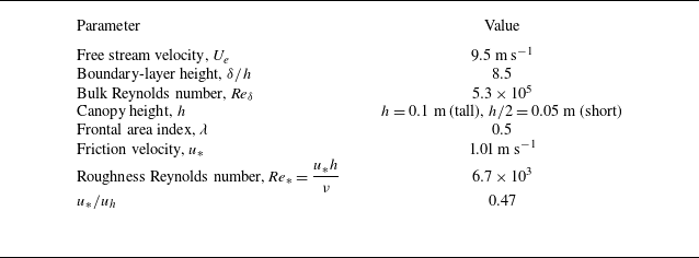

 σu
 σw
 z/h=1
 z/h=1.2

 u′w′¯
 νt=−u′w′¯/∂u¯/∂z
 ΔSuw

 cmax/cs

 y/h=0
 c¯/c¯max
 σc/c¯max
 c¯max/cs

 ic
 c99/σc
 γc
 M3c

 M3c
 ic
 M4c
 M3c
 M3c=a1ic+a2ic−1
 M4c=b1M3cb2+b3
 Γ

 c/σc
 Γ
 z/h=2.4
 z/h=1.6
 z/h=1.2
 N1,0
 N2,0
 F1,0
 F2,0

 w′c′¯
 c¯/cmax
 N1,0
 N2,0
 F1,0
 F2,0
 h

 Dt=−((w′c′¯)/(∂c¯/∂z))
 N1,0
 N2,0
 F1,0
 F2,0

 Sct
 N1,0
 N2,0
 F1,0
 F2,0

 rxy=x^y^¯

 w′c′¯ q
 N1,0
 N2,0
 F1,0
 F2,0

 Ewc
 Euw
 N1,0
 N2,0
 F1,0
 F2,0

 w′c′¯
 N1,0
 N2,0
 F1,0
 F2,0

 w^2c^¯
 u^w^c^¯
 N1,0
 N2,0
 F1,0
 F2,0

 ΔSwc
 u^w^c^¯
 w^2c^¯
 u^w^c^¯=αw^2c^¯
 w′w′c′¯
 0.8≤z/h≤3.5
 y/h=0
 y/h=0.5

 ΔSwc
 N1,0
 N2,0
 F1,0
 F2,0
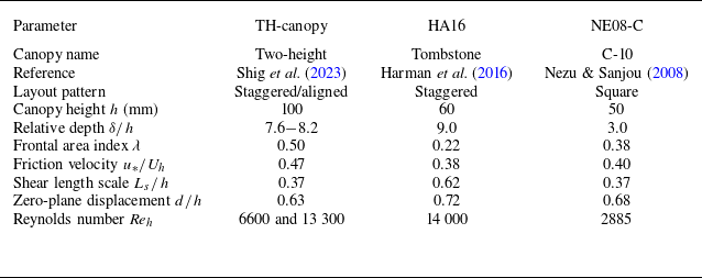
 ν≈1.0×10⁻⁶
 2
 −1
 ν≈1.5×10⁻⁵
 2
 −1

 u¯/uh
 −u′w′¯/u∗
 σu/u∗
 −σw/u∗
 z/h={0.5,1.0}

 F1,2

 ⟨u¯⟩/uh
 −⟨u′w′¯⟩/u∗2
 σu/u∗
 σw/u∗
 u′w′¯4/u′w′¯2
 z/h={0.5,1.0}

 S2,0
 N2,0
 F2,0
 u¯/u∗
 −u′w′¯/u∗2
 σu/u∗
 σw/u∗
 z/h={0.5,1.0}
 %

 Open access

