2.1 Shortest path

Path planning should derive the shortest route to the target point, and it is essential to minimise the time required to derive the route. Many methods have been used to establish path planning, such as visibility graphs, waypoint graphs and grid methods.

A visibility graph is a set of adjacency matrices for each connection node and distance information. The nodes of the visibility graph are composed of the starting point, target point and vertices of the obstacle, and the link is composed of visible lines between the nodes. The visibility graph guarantees the shortest path by using the links connecting the nodes. However, because the vertex of an obstacle is used, there is no free space in the moving path (Wang and Guo, Reference Wang and Guo2003; Zhang et al., Reference Zhang, Liu, Liu and Hu2008). Therefore, realistically, the arrival of a rescue vessel at an obstacle node indicates a collision or stranding on an island or aquaculture farm. Meanwhile, in waypoint graphs, an edge between two waypoints indicates that the rescue ships can pass through this point safely without colliding with the region boundaries or obstructions. However, waypoint graphs do not guarantee a short distance because they do not use vertices as nodes, but instead place them at random midpoints between obstacles (Zhu et al., Reference Zhu, Jia, Wan, Yang, Hu, Qin and Cui2015). In places where various aquaculture farms, such as abalone and seaweed farms, are scattered, the corners of the farms become hundreds of thousands or millions of nodes. Therefore, there is a problem with the amount of computation required in methods such as visibility and waypoint graphs.

Meanwhile, a grid-based node can be analysed using a detailed and consistent principle, and is particularly suitable for analysing a considerable area characterised by an open-space configuration (Akbari et al., Reference Akbari, Pelot and Eiselt2018b; Lin et al., Reference Lin, Song, Gui, Wang and Su2018). A rescue ship cannot stand still in one place, unlike a car, due to the tide, so a small drifting zone is needed for emergency response to a marine accident. Therefore, a study is required to determine the optimal location based on the grid. We chose a grid-based method in this study.

2.2 Optimisation

The placement problem is a classic optimisation problem that identifies the optimal site for a facility based on geographical requirements and transportation distances. As the location model becomes increasingly sophisticated, such as the set covering location model (SCLM) and p-median model (PMM), it has proven to be NP-hard (Megiddo and Supowit, Reference Megiddo and Supowit1984). Increasing the problem size makes it difficult for traditional optimisation approaches to handle these challenges. Therefore, diverse intelligence methods, such as PSO, genetic algorithms and the simulated annealing algorithm, have been used to solve challenging large-scale location problems (Qin et al., Reference Qin, Ni and Shi2012; Alnahhal and Noche, Reference Alnahhal and Noche2015; Adeh et al., Reference Adeh, Baroughi and Alizadeh2017).

The PSO algorithm is an evolutionary algorithm developed by Kennedy and Eberhart (Reference Kennedy and Eberhart1995). This optimisation technique simulates the movement of swarms of insects, birds and fish through information exchange and cooperation. Unlike other heuristic algorithms, the PSO algorithm can overcome the shortcomings of early convergence to a local solution by balancing the global and local solutions in the search space. In addition, there are advantages in that the algorithm is simple, has a relatively small number of parameters and can be implemented with simple computer coding. Therefore, in this study, PSO was applied to metaheuristic optimisation methods to efficiently determine the optimal position among the candidate positions.

3.1 Preparation for modelling

The space to be analysed is divided into grids. Each grid is set as a node, which is the candidate location for the rescue ship. The graph is a set of adjacency matrices of each connection pair and distance information, including information on connection pairs that have a relationship with the nodes. Nodes on land, aquaculture farms, shorelines and obstacles other than the sea are excluded from the node candidates.

Knowing that an accident occurs in a specific area does not mean that it will happen again in the same place, nor does it mean that the accident cannot be in another location if it did not happen in the past. Therefore, it is appropriate to simulate the distribution of potential accidents in the study area using statistical estimates from historical data to address this problem. Furthermore, because patterns of past accidents are potent predictors of the future, it is essential to extract the underlying distributions of the positions of past accidents as the basis for a probabilistic approach to generating future accidents (Akbari et al., Reference Akbari, Eiselt and Pelot2018a, Reference Akbari, Pelot and Eiselt2018b). The extraction of distributions from past accidents can be accomplished using a two-dimensional kernel density estimator (KDE), which is a non-parametric method for estimating the probability density function.

3.2 Objective function

In this study, we consider two classic location models, SCLM and PMM, which are adjusted and applied to our problem characteristics. SCLM determines the rescue ship location and the required vessels (Roth, Reference Roth1969; Toregas et al., Reference Toregas, Swain, ReVelle and Bergman1971). SCLM ensures that every demand point is covered at least once. PMM minimises the total or average distance between p facilities and every demand location (Hakimi, Reference Hakimi1965).

The objective functions of SCLM and PMM were designed such that all marine accidents can be serviced within a given time. First, a rescue ship was dispatched close to the marine accident location. If there is only one rescue ship owing to bad weather or repair of a rescue ship in the jurisdictional area, the constraint condition is designed to arrive within 1⋅5 h based on a maximum speed of 30 knots. However, in the case of two or more rescue ships, the constraint condition was designed such that it could be reached within 1 h.

The objective function for the SCLM is given by Equation (1) (Caprara et al., Reference Caprara, Toth and Fischetti2000). Let ${c_r}$ denote the r-th grid node location for the rescue ship, which is the starting point. In addition, ${y_m}$ denotes the $m$-th grid node location for an estimated marine accident site, which is a destination.

(1)\begin{equation}argmi{n_{{c_1},\; {c_2},\; \ldots\; ,\; {c_r}}}\left\{ {\mathop \sum \limits_{m = 1}^l \textrm{min}({||{{c_1} - {y_m}} ||,||{{c_2} - {y_m}} ||, \cdots ,||{{c_r} - {y_m}} ||})}\right\}\end{equation}

subject to

\[\textrm{min}({||{{c_1} - {y_m}} ||,||{{c_2} - {y_m}} ||, \cdots ,||{{c_r} - {y_m}} ||} )\mathrm{\ < }\theta \textrm{,}\,\theta =\left\{ {\begin{array}{@{}ll@{}} {\textrm{45}\,\textrm{nm}}& {\textrm{for}\ r=1}\\ {\textrm{30}\,\textrm{nm}}& {\textrm{otherwise}} \end{array}} \right.\]

Here, $||\cdot ||$ is calculated by the theory of the spherical law of cosines using Equation (2) (Ramachandran et al., Reference Ramachandran, Deshpande, Roseman, Rosenberg, Feldman and Cavalli-Sforza2005). Let $p_g^{lat}$ and $p_g^{lon}$ denote GPS latitude and longitude at the g-th node, respectively, and $p_{g + 1}^{lat}$ and $\; p_{g + 1}^{lon}$ indicate those respective coordinates at the next node.

(2)\begin{equation}||\cdot ||= \mathop \sum \limits_{g = 1}^G e\; \textrm{arcos\{sin(}p_g^{lat}\textrm{) sin(}p_{g + 1}^{lat}\textrm{) + cos(}p_g^{lat}\textrm{) cos(}p_{g + 1}^{lat}\textrm{) cos(}p_g^{lon} - p_{g + 1}^{lon}\textrm{)\} }\end{equation}

where $||\cdot ||$ is the sum of distances between nodes. The shortest distance means that the destination is reached through several waypoints from the starting point. Here, G represents the total number of nodes, including the starting node, several waypoint nodes and the destination node. Additionally, G is two if it is possible to go directly from the starting point to the destination without obstacles and e denotes Earth's radius.

Unlike SCLM, PMM considers the estimated probability density required to reflect marine accident demands. The estimated probability density of each grid can be calculated using the KDE from historical marine accidents. The estimated probability density is used as the demand weight in the objective function. The objective function for PMM is given by Equation (3) (Mladenović et al., Reference Mladenović, Brimberg, Hansen and Moreno-Pérez2007). The objective function serves to find the location of rescue ships in the jurisdictional area with the shortest cumulative distance for all marine accident demands. Here, $\tau ({{y_m}} )$ is the density of the accidents estimated using the KDE at the $m$-th grid node and l is the total number of candidate nodes for the rescue ship arrangement.

(3)\begin{equation}argmi{n_{{c_1},\; {c_2},\; \ldots\; ,\; {c_r}}}\left\{ {\mathop \sum \limits_{m = 1}^l \textrm{min}({||{{c_1} - {y_m}} ||,||{{c_2} - {y_m}} ||, \cdots ,||{{c_r} - {y_m}} ||} )\; \tau ({{y_m}} )\; } \!\right\}\end{equation}

subject to

\[\textrm{min}({||{{c_1} - {y_m}} ||,||{{c_2} - {y_m}} ||, \cdots ,||{{c_r} - {y_m}} ||} )\mathrm{\ < }\theta , \,\theta =\left\{ {\begin{array}{*{20}{l}} {\textrm{45 nm}}& {\; \; \textrm{for}\; r = 1}\\ {\textrm{30 nm}}& {\; \textrm{otherwise}} \end{array}} \right.\]

where $\tau ({{y_m}} ) = \frac{1}{{N{b^2}}}\mathop \sum \limits_{n = 1}^N \varphi \left( {\frac{{{y_m}-{z_n}}}{b}} \right)$, N is the number of marine accidents in the study area, ${z_n}$ denotes the location of an n-th actual marine accident and $\varphi$ is the kernel function. A Gaussian kernel is used to estimate the density function and b indicates the bandwidth. A horizontal grid spacing was used as the bandwidth.

3.3 Comparison criteria

It is essential to arrive at a site within the golden time to save life. The access time, also referred to as the response time for marine accidents, can be minimised by shortening the voyage distance depending on the location of the rescue ships. The average access time is frequently used as a model criterion in location studies (Akbari et al., Reference Akbari, Eiselt and Pelot2018a). This criterion assesses the time required for the nearest response vessel to arrive at a marine accident site, as given by (Akbari et al., Reference Akbari, Pelot and Eiselt2018b)

(4)\begin{equation}\textrm{Average}\,\textrm{access}\,\textrm{time = }\frac{1}{T}\mathop \sum \limits_{t = 1}^T \frac{{{d_t}}}{h}\end{equation}

where ${d_t}$ is the distance between the closest rescue ship and t-th marine accident demand, T is the total marine accident demand and h is the speed of the rescue ship.

3.4 Dynamic programming

DP methods are applied to determine the shortest distance between a rescue ship and a marine accident. DP is used extensively in optimisation problems (Bellman, Reference Bellman1966). The shortest-path problem has an optimal substructure. For example, suppose s → u → v is the shortest path from s to v. Node s for a rescue ship, which is the start position; node v for a marine accident, which is the destination; and node u for waypoints. The shortest path from node s to node v that uses only up to u intermediate nodes is the shortest path that either does not use node u at all or consists of the merging of the two path node s to node u and node u to node v. Let ${\delta _k}({s,\; v} )$ be the shortest s → v path using $\le$k edges. This problem is similar to finding several paths from a rescue ship position to a marine accident with k edges, in which we have to find the total number of paths. Therefore, for this problem, the shortest path is one of the paths with the lowest distance. Based on this optimal substructure, we can determine the recursive Equation (5) of the single-source shortest path problem as follows (Denardo, Reference Denardo2012):

(5)\begin{equation}{\delta _k}({s,\; v} )=\min \{ {\delta _{k - 1}}({s,\; v} ),\; {\delta _{k - 1}}({s,\; u} )+ {\delta _{k - 1}}({u,v} )\; \textrm{|}({u,\; v} )\in E\} \end{equation}

This step initialises the distances from the rescue ship to marine accidents as infinite and the distance to the rescue ship itself as 0. The base cases are

\[{\delta _0}({s,\; v} )=\infty \ \textrm{for}\ v \ne s\]

\[{\delta _k}({s,\; s} )=0\ \textrm{for}\ \textrm{any}\ k=0\ \textrm{for}\ \textrm{any}\ k\]

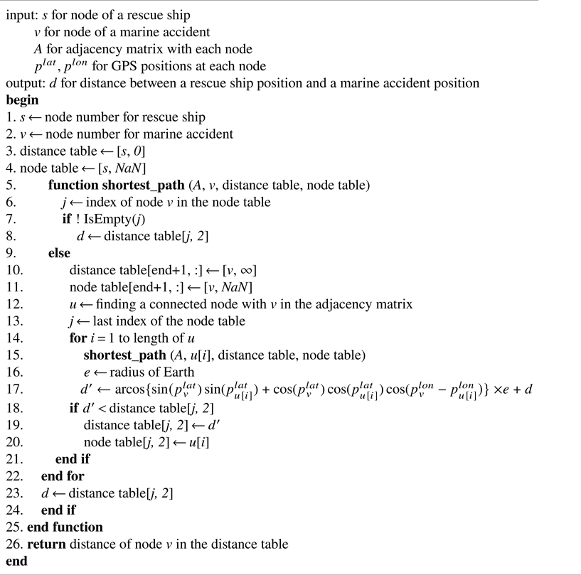
We use an adjacency matrix to represent the edge information if an edge between two arbitrary nodes is connected in the graph. If there is an edge from node s to node v in the graph, the value is 1; if there are no edges from node s to node v in the graph, the value is 0. Some accidents within the aquaculture farms may not have connectable nodes. These accidents were resolved by relocating to the nearest connectable node. The distance between two nodes is calculated using the spherical law of cosines based on the GPS coordinates formed by two components: latitude, giving the north-south position, and longitude, giving the east-west position (Ramachandran et al., Reference Ramachandran, Deshpande, Roseman, Rosenberg, Feldman and Cavalli-Sforza2005). The unit of distance was converted to nautical miles (nm). The following Algorithm 1 of DP was used to compute the shortest path.

Algorithm 1.

Shortest path with dynamic programming.

Algorithm 2.

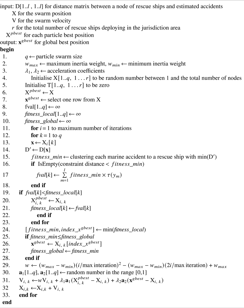
Particle swarm optimisation for PMM.

3.5 Particle swarm optimisation

The total number of candidate nodes for rescue ships is l. All possible combinations of the number of rescue ships r elements out of the total number of candidate nodes l are countless. Therefore, we randomly sampled with a particle swarm size (q) among the total number of candidate nodes to apply PSO. The sampled matrix, $\textrm{X}$, indicates the initial particle swarm position. Subsequently, the position and velocity of each particle were updated repeatedly. Therefore, each particle has a fitness value calculated using a fitness function and finds the best position. The best position of each particle, which is the local best, is integrated into one matrix, ${\textrm{X}^{pbest}}$. The global best position of the entire swarm is denoted by $\textbf{x}_{}^{gbest}=({{x_1},\; {x_2},\; \ldots , \; {x_r}} )$. In particular, the velocity of a particle is influenced by certain components. First, the inertia weight (w) determines the confidence of a particle in its movement, which is unaffected by ${\textrm{X}^{pbest}}$ and ${\textbf{x}^{gbest}}$. Second, the acceleration coefficients (${\lambda _1}$, ${\lambda _2}$) determine the extent to which a particle is influenced by the memory of its best solution.

Shi and Eberhart showed that PSO with linearly decreasing inertia weight performs better than PSO with fixed inertia weight (Shi and Eberhart, Reference Shi and Eberhart1998). They varied the inertia weight linearly from 0⋅9 (${w_{\textrm{max}}}$) to 0⋅4 (${w_{\textrm{min}}}$) in the run and fixed the acceleration coefficients (${\lambda _1}$, ${\lambda _2}$) at 2⋅0 (Shi and Eberhart, Reference Shi and Eberhart1999). Here, w is an inertia weight that adjusts the strength of the previous velocity with respect to the current velocity and plays an essential role in the convergence of the PSO algorithm. If the inertia weight is significant, the global search is strengthened; if it is set to a small value, the local search is intensified. However, a global solution may not be obtained if an inappropriate value is selected. Various methods exist for determining inertia weight (Tian and Shi, Reference Tian and Shi2018). This study chose inertia weight as a significant value at the beginning of the search, and the inertia weight decreased nonlinearly as the search proceeded. The global search was strengthened in the initial stage and, as the iterations progressed closer to the optimal solution, the local search was given more weight (Guimin et al., Reference Guimin, Jianyuan and Qi2006). The following Algorithm 2 uses PSO to efficiently find the optimal position for PMM.

4.1 Data collection

The area under study, namely the Wando County, South Korea, comprises 264 islands. In addition, a national marine park is situated in the coastal waters of Wando, Jeollanam Province. This park is an active seaweed farm in the South Korean coastal waters. Furthermore, 80% of South Korea's abalone production is produced in Wando County. Consequently, there are 8,100 fishing vessels in this region (Ock, Reference Ock2010; Yoo and Jung, Reference Yoo and Jung2017).

The open ocean of Wando in the South Sea of Korea is one of the most significant shipping regions in the world, connecting China, Japan, Russia and South Korea. Consequently, an increase in the volume of vessel traffic results in a proportional increase in the number of marine accidents. In particular, approximately 2,000 Chinese fishing boats navigate through this area for fishing in eastern North Korea every year. As a result, near collisions with merchant ships occurred frequently, with a total of three collisions. The research region consists of multiple islands and a complex coastline located between latitudes 33⋅9° and 34⋅6° north and longitudes 126⋅2° and 127⋅2° east.

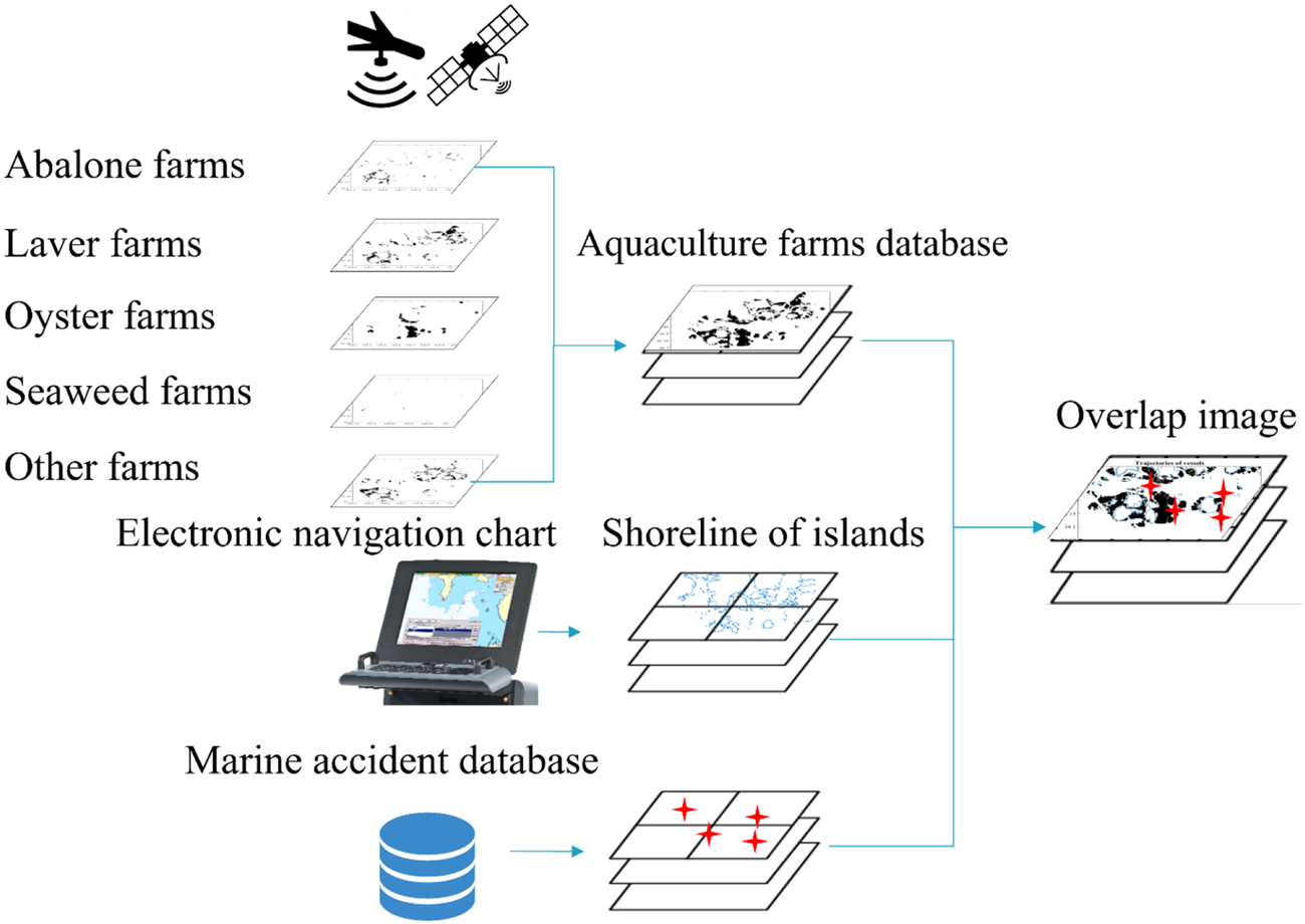
Figure 1 shows the process of overlaying the three databases. First, satellite and aerial photographs of the study area were processed to determine the locations of the aquaculture farms. In this procedure, we constructed an integrated aquaculture farm database after collecting data for abalone, laver, oyster, seaweed, etc. (Yoo and Jung, Reference Yoo and Jung2017). Second, the coastline of the research area was obtained from electronic navigational charts (ENC). Third, we analysed marine accidents between 1997 and 2016 on numerous islands in Wando County, South Korea (KMST, 2016).

Figure 1.

Procedure of overlaying three databases: aquacultures, shorelines of islands and marine accidents

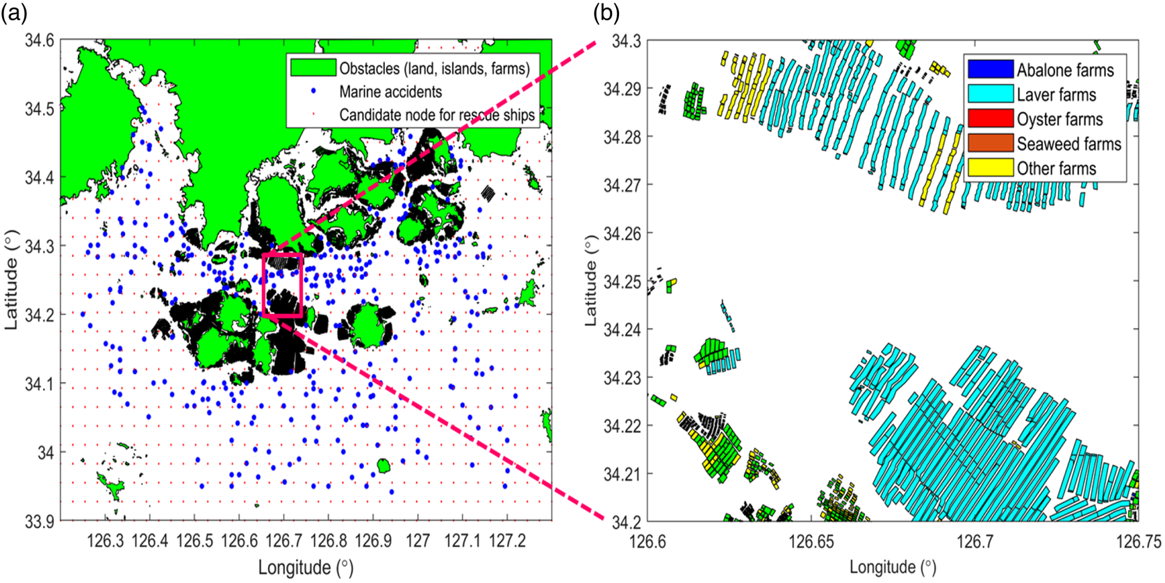
Three coast guard rescue ships were specifically stationed in this maritime area for search and rescue operations. The nearest of the three rescue ships was allocated to the rescue mission and dispatched immediately to the accident location. We spaced the grid node in the study area and marked it as a candidate node for the rescue ship in the absence of obstacles. We set the grid node interval to 1⋅65 nm in the direction of the longitude and latitude in the study area. Figure 2(a) shows a scatter plot of the candidate nodes for rescue ships on the grid (red dots) and marine accidents (blue dots) in the study area. Figure 2(b) shows the distribution plot of the integrated aquaculture farms, including abalone, laver, oyster, seaweed farms, etc.

Figure 2.

Study area: (a) scatter plot of the candidate nodes for rescue ships on the grid (red dots) and marine accidents (blue dots); (b) distribution plot of the integrated aquaculture farms

4.2 Future demand using kernel density estimation

The assumptions considered in this study are as follows.

1. (1) The average speed from the location of the rescue ship to the site of the marine accident was the same for all rescue ships.

2. (2) If only one rescue vessel is deployed in the waters under jurisdiction, the time required to arrive at the accident should be within 1⋅5 h. If two or more ships are deployed, the time required should be within 1 h.

3. (3) Marine weather, such as wind speed, wind direction, current speed, current direction and wave height, was not reflected.

4. (4) After the rescue ship received the marine accident report, the time to prepare for the travel movement was not considered.

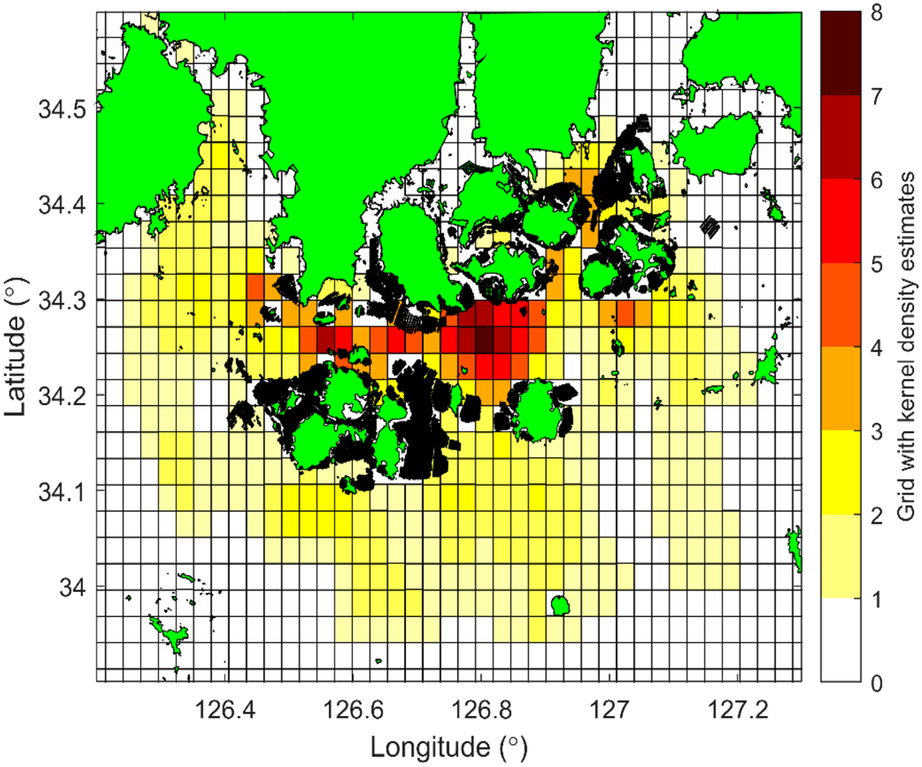
Kernel density estimates serve the demand for generating random marine accidents in future scenarios. Using past marine accidents to predict future demand, as most studies have done, implies that the future will behave identically to the past. In the study region, 439 marine accidents have occurred over the past two decades. The density estimates applied in this study were calculated based on collisions, grounding, fires, explosions, engine failures, steering gear damage and floating object accidents, and the weights for each factor were not considered. This is because, regardless of the severity of any marine accident, rescue ships guarding within their jurisdiction are obliged to go to the accident site when a report is received (Figure 3).

Figure 3.

Kernel estimates for marine accidents on a gridded map

For the kernel density calculations, the centre of each grid, which is the candidate node for stationing rescue ships, was used. A Gaussian kernel was used for the density estimation. The bandwidth b of a kernel function is applied as a grid cell size of 1⋅65 nm. Figure 4 shows each kernel density estimate at the centre of the grid cell. In total, 1,030 marine accidents were estimated to occur in the study area. The density estimate of marine accidents is shown to be high at 34⋅2° to 34⋅3° N, where ship traffic is frequent.

Figure 4.

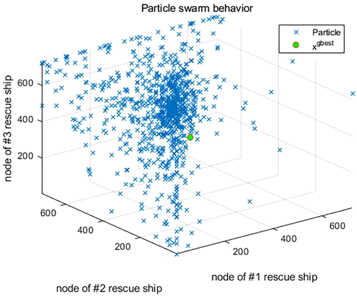
Scatter plot for the position of the particle swarm at the initial iteration for PMM; the initial position of each particle is indicated with a blue cross mark and the global position with a green circle

4.3 Performance evaluation

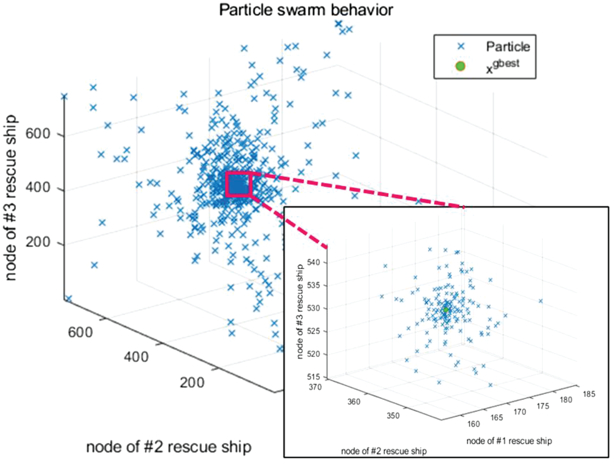
The program was executed on a PC with an Intel Xeon E5-2650 v3 processor (10 CPU cores, 16 × 8 GB DDR4 RAM, 2⋅3 GHz). We set the particle swarm size (q) parameter to 1,000 and the number of iterations to 100. Figure 4 shows a scatter plot of the initial position of the particle swarm at the initial iteration for the PMM when the three rescue ships were deployed. Figure 5 shows a scatter plot of the last position of the particle swarm and the global best at the last iteration under the same conditions. As the number of iterations increased, the diverged particles converged around the global best solution. The global best solution for the PMM was ${\textbf{x}^{gbest}}$ = (177, 365, 526).

Figure 5.

Scatter plot for the position of the particle swarm at the last iteration for PMM; the last position of each particle is indicated with a blue cross mark and the global best position with a green circle

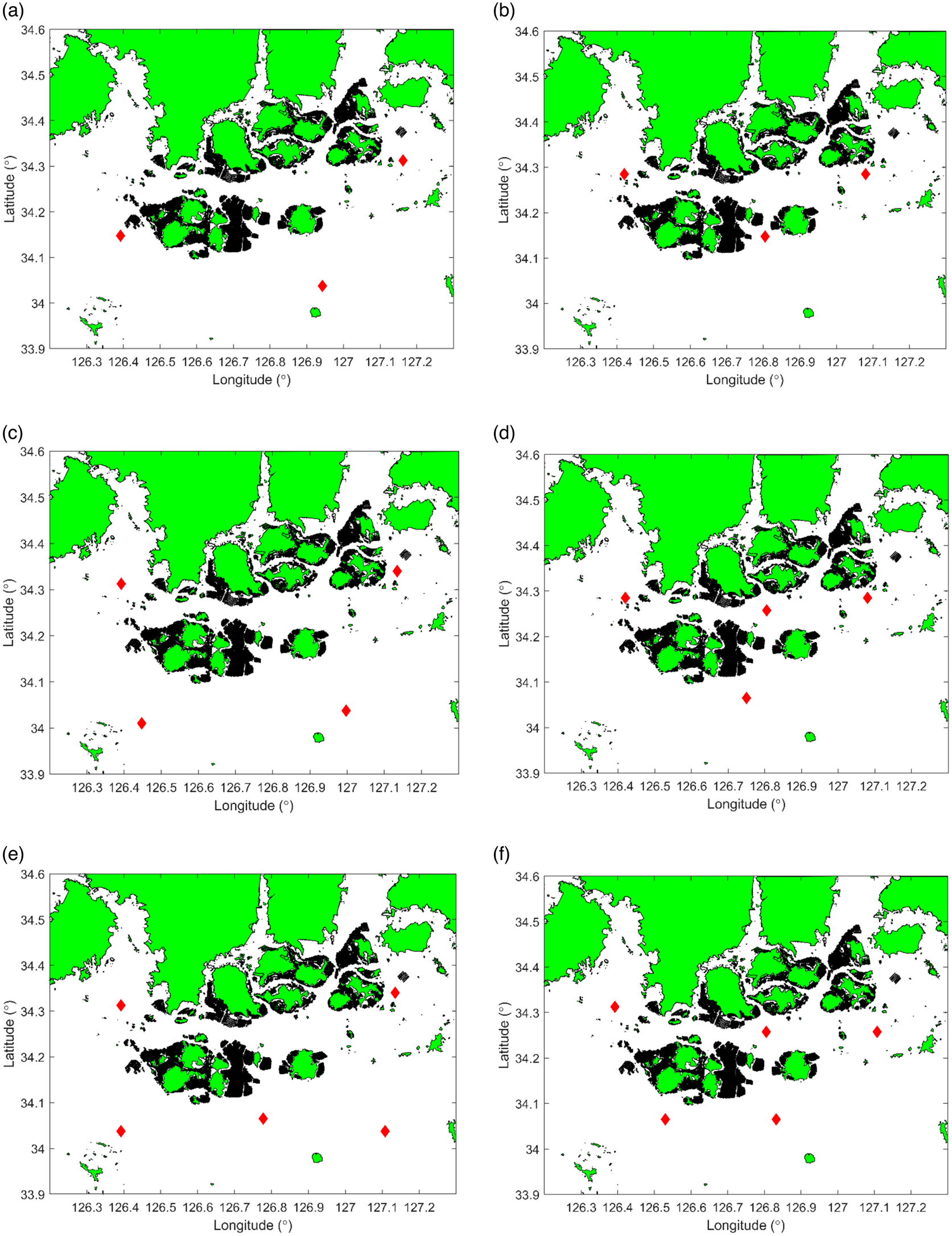
Table 1 lists the average access time to the location of future marine accidents based on the number of rescue ships. When only one or two rescue ships were deployed, the optimal locations based on SCLM and PMM were the same, resulting in the same average access time. However, when more than three rescue ships were deployed, the average access time differed by more than 3 min.

Table 1.

Comparative experiments with an average access time (m) for SCLM and PMM

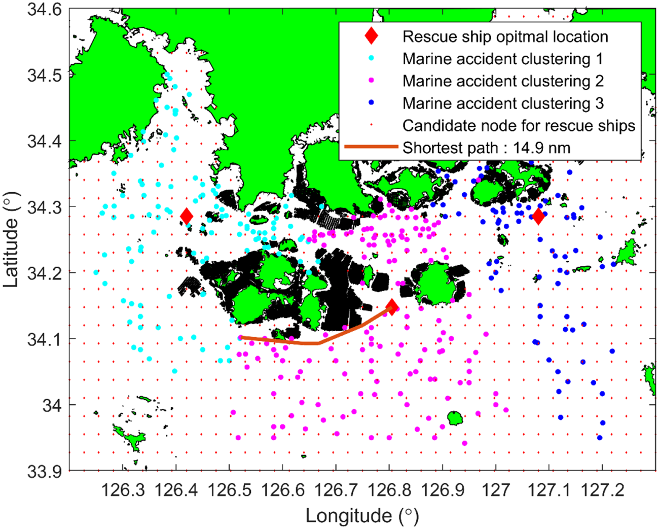
Figure 6 shows the candidate nodes for deploying rescue ships (red dots) and the optimal locations for rescue ships based on PMM (red diamonds) in the study area. Marine accidents were naturally allocated and clustered to rescue ships in cyan, magenta and blue. This suggests that the jurisdiction of each rescue ship could be divided. The brown line indicates the shortest path that detours around obstacles from a rescue ship to a marine accident. The sample in Figure 6 shows the distance of 14⋅9 nm from a rescue ship to a marine accident. It can be confirmed that the closest rescue ship reached the marine accident at the shortest distance by navigating around obstacles such as islands and fish farms.

Figure 6.

Optimal locations for rescue ships (red diamonds) based on PMM, candidate node for deploying a rescue ship (red dot), actual marine accident location clusters (cyan, magenta, blue) and shortest path from a rescue ship to a marine accident (brown line)

Figure 7 shows the optimal location based on SCLM and PMM. According to Figure 3, there is a high demand for marine accidents at 34⋅2° to 34⋅3° N. Therefore, the optimal location of the PMM-based two or three rescue ships is arranged at 34⋅2° to 34⋅3° N in Figures 7(b), 7(d) and 7(f). Conversely, the location of the SCLM-based rescue ship is arranged such that it can arrive within a limited time of 1 h. Therefore, a sufficient distance is maintained between the rescue ships such that at least one rescue ship is assigned to any location of a possible marine accident.

Figure 7.

(a), (c) and (e) Optimal locations (red diamonds) of the SCLM-based on the number of rescue ships. (b), (d) and (f) Optimal locations (red diamonds) of the PMM-based model by the number of rescue ships