




1. Introduction and main results
The main motivation for this work came from the author’s conversations with K. A. Landman concerning certain mathematical tissue growth models she was developing with her co-authors some time ago [Reference Binder, Landman and Simpson5, Reference Binder and Landman6]. One of the purposes of the models was to better understand the neural crest invasion process, which occurs during embryogenesis and leads to the formation of the enteric nervous system in the intestine of vertebrates. A major contributing factor to that process is gut growth; of interest is understanding the position and speed of the wavefront with time, and tracking individual cells or small groups of cells at different positions in the wave. Idealizing the developing three-dimensional gut tissue as a series of cylindrical shells, the authors of [Reference Binder, Landman and Simpson5] assumed further that ‘the thickening of the cross-sectional area is small compared to the elongation and radial expansion, so that the overall growth can be approximated by the increase in the area of the outer cylindrical surface. Each cylindrical shell is cut lengthwise, so becoming a flat rectangular plate with a fixed thickness’. The basic model only considers uniaxial growth, the width of the rectangular plate remaining constant.
The key element of the basic approach discussed in [Reference Binder, Landman and Simpson5, Reference Binder and Landman6] is the following continuous-time one-dimensional cellular agent model. Suppose we start with  $L(0)=N$ agents located at the integer points
 $1,2,\ldots, L(0)$ on the real line. Assume that
 $d\ge 1$ of the initial N agents are marked, and we are interested in tracking the movement of these marked agents as the tissue grows. The agents are allowed to proliferate, by mitotic division. At the end of an agent’s life it splits into two (modelling mitotic division of cells), the daughter agents being inserted in the ‘linear tissue’ instead of the mother. If the latter was at location i at its division time
 $t>0$, then its daughters will be placed at locations i and
 $i+1$, while all the agents that prior to that division event were at locations
 $i+1,i+2, \ldots, L(t{-})$ will be pushed one step to the right, to the respective locations
 $i+2,i+3, \ldots, L(t)=L(t{-})+1$. For the sake of definiteness, if the mother agent was marked, the mark is inherited by the ‘right daughter’ (the one at location
 $i+1$) only, so that at all times there will still be exactly d marked agents.
The lifetimes of the agents are assumed to be independent exponential random variables with a common rate  $\lambda >0$, so that the dynamics of L(t) is that of a pure birth process with the birth rate
 $\lambda k$ given
 $L(t)=k$. This is the well-known Yule process. The dynamics of the process are well understood: it is basically exponential growth; see, e.g., [Reference de La Fortelle12] and references therein.
It is easy to see that the dynamics of the locations of the d marked cells can be reduced to that of a  $(d+1)$-color Pólya urn process. Denote the locations of the d marked agents immediately after the nth division event by
 $ M_1(n) <M_2 (n) <\cdots <M_d (n) $, their initial values being
 $M_j(0)=N_j$,
 $j=1,\ldots , d$, where
 $0\,=\!:\,N_0 <N_1<N_2 <\cdots <N_d <N\,=\!:\,N_{d+1}$, and set for notational convenience
 $M_0(n)\,\,:\!=\,\,0$,
 $M_{d+1}(n)\,\,:\!=\,\, N+n$. As the rates of all the agents’ exponential lifetimes are the same, all the currently existing agents are equally likely to become the next cell to divide. Interpreting the
 $\xi_j(n)\,\,:\!=\,\,M_j(n)-M_{j-1}(n)$,
 $j=1,\ldots, d+1$, agents located at the integer points within the half-open interval
 $(M_{j-1}(n),M_j(n)]$ as ‘balls of color j’ after n steps in an urn model, we see that the dynamics of
 \begin{align}\{\boldsymbol{\xi}(n)\,:\!=\, (\xi_1(n),\ldots, \xi_{d+1} (n))\,:\, n\ge 0\}\end{align}
are those of a simple  $(d+1)$-color Pólya urn, where at each step a ball is extracted at random from the urn and then returned with one more ball of the same color. This reduction was noted in [Reference Binder, Landman and Simpson5] in the case of
 $d=1$. In fact, the reverse ‘embedding’ of discrete-time urn schemes into Markovian continuous-time models had already been used, about fifty years ago, in [Reference Athreya and Ney1] (see also Section 4 in [Reference Athreya and Ney2] and the general discussion in [Reference Blom and Holst8]), and more recently was successfully revisited and further developed in [Reference Janson18, Reference Janson19].
To analyze the cellular agents model, the authors of [Reference Binder and Landman6] ran simulations, starting with  $N=24$ initial agents. The results showed emergence of bell-shaped distribution curves (quite Gaussian in their shape) for the marked agents’ locations after a few tens of divisions. Then, using the conditional (given the current urn composition) first and second moments of the one-step increments of the number of balls of a given color in a two-color (i.e. when
 $d=1$) continuous-time Pólya urn model, the authors wrote down the Fokker–Planck equation with the same infinitesimal drift and diffusion coefficients. The plots of the univariate densities of the corresponding diffusion process proved to be in excellent agreement with the simulation results, suggesting that the heuristic approach used indicated a valid mathematical approximation result.
In the present paper, we establish Gaussian process approximations to the trajectories of the locations of  $d\ge 1$ marked agents in the uniaxial growth cellular agent model, under the most relevant to the above motivation scenario where the initial number of cells N is large ([Reference Binder and Landman6] mentions that in quail, the cell number in the small plus large intestine is around 800 000 at an embryonic age of four days, and increases approximately five-fold in the next three days). We measure time in terms of the number of cell divisions
 $n\to\infty$ rather than using the ‘physical time’ t (to which the transition is quite straightforward). In other words, we provide approximations to the dynamics of
 $(d+1)$-color Pólya urn models, as both the initial number of balls N and the number n of draws tend to infinity. These results are based in the strong approximation established in Theorem 1 and are stated in Corollary 1. To be more precise, the approximations established there are uniform for the whole family of Pólya urn processes with
 $N\to\infty$ initial balls and all possible values of d and initial urn compositions. Furthermore, in Theorem 2 we establish a uniform bound for the rate of convergence of the distribution of the time n locations of the d marked agents (or, equivalently, for the urn composition after n draws) to the respective normal distribution on
 $\mathbb{R}^d$.
There is a vast literature devoted to studying the behavior of what are nowadays called ‘Pólya urn models’ and their generalizations. In its basic form, the model was introduced in 1906 in Section 4 of the very first paper on chain dependence by A. A. Markov [Reference Markov24]. It was used there as an example of a sequence of dependent random variables for which the weak law of large numbers did not hold. The standard reference being [Reference Eggenberger and Pólya14], the reader is further referred to [Reference Johnson and Kotz20, Reference Kotz and Balakrishnan22, Reference Mahmoud23] for surveys of results concerning urn models. We already mentioned [Reference Janson18], which, using the Athreya–Karlin embedding idea from [Reference Athreya and Ney1], establishes several limit theorems for the numbers of balls in generalized two-color Pólya urn schemes and provides references to earlier work in that direction. Until very recently, no limit theorems were available in the case of large numbers of initial balls, which is important for us. After this paper appeared in the arXiv preprint repository, the author was notified of [Reference Cheliotis and Kouloumpou9] where the behavior of two-color Pólya urns was considered under the assumption that the initial total number of balls goes to infinity. In particular, Theorem 1.4 in [Reference Cheliotis and Kouloumpou9] presents a weak convergence result as  $n\to\infty$ for a centred and scaled version of the processes
 $\boldsymbol{\xi} (\lfloor nt\rfloor)$ under the assumption that
 $d=1$,
 $\xi_1 (0) = \lfloor an + \theta_1 n^{1/2}\rfloor $,
 $\xi_2 (0) = \lfloor bn + \theta_2 n^{1/2}\rfloor $ for some constants a, b,
 $\theta_1 $, and
 $ \theta_2$. This result is related to our Corollary 1(ii).
Now we will turn to formulating our main results. We start by recalling that one of the key classical results for the basic two-color Pólya urns is the almost sure (a.s.) convergence (as the number of draws n goes to infinity) of the proportion of the balls of a given color to a beta-distributed random variable (and we note that it was shown in [Reference Goldstein and Reinert15] that the rate of the distributional convergence in the Wasserstein metric is  $O(n^{-1})$, with a constant depending on the initial composition of the urn). A similar convergence result holds for multicolor urn models as well. For
 ${\alpha} \,:\!=\, (\alpha_1 ,\ldots, \alpha_{d+1} )\in \mathbb{N}^{d+1}_{>0}$, denote by
 $\boldsymbol{\xi}^{\boldsymbol{\alpha}} (n)$ the value of the
 $(d+1)$-color Pólya urn process (1) after n draws, given that it started at the initial vector
 $\boldsymbol{\xi}^{\boldsymbol{\alpha}} (0) =\boldsymbol{\alpha}$ (note that the dimensionality of the superscript gives the number of colors in the model and so completely specifies the latter; for brevity, the superscript
 $\boldsymbol{\alpha}$ will mostly be omitted in what follows). Then, for the vector of the proportions of balls of different colors after n draws, we have
 \begin{equation}\boldsymbol{\xi}^{\boldsymbol{\alpha}} (n)/(N+n)\stackrel{\footnotesize\mbox{a.s.}}{\longrightarrow} {\textbf{\textit{V}}}^{\boldsymbol{\alpha}} \qquad \mbox{as } n\to\infty,\end{equation}
where  $N =\sum_{j=1}^{d+1} \alpha_j$ and the limiting random vector
 ${\textbf{\textit{V}}}^{\boldsymbol{\alpha}} $ (for which we will also often omit the superscript
 $\boldsymbol{\alpha}$, writing just
 ${\textbf{\textit{V}}}=(V_1,\ldots,V_{d+1})$) follows the Dirichlet distribution
 $\mbox{Dir}_{d+1}(\boldsymbol{\alpha})$ with parameters
 $(\alpha_1, \ldots,\alpha_{d+1})$ (see [Reference Blackwell and MacQueen7]; note that the a.s. convergence here is a chrestomathic consequence of the martingale convergence theorem). Introducing the notations
 ${\textbf{\textit{x}}}^{\#}\,:\!=\, (x_1, \ldots, x_{d})\in \mathbb{R}^{d}$ for
 ${\textbf{\textit{x}}}=(x_1, \ldots, x_d, x_{d+1} )\in \mathbb{R}^{d+1}$ and
 $B^{\#}\,:\!=\, \{{\textbf{\textit{x}}}^{\#}\,:\, {\textbf{\textit{x}}}\in B\}$ for
 $B\in \mathbb{R}^{d+1}$, recall that
 $\mbox{Dir}_{d+1}(\boldsymbol{\alpha})$ is concentrated on the standard simplex
 $\Delta^d\,:\!=\,\bigl\{{\textbf{\textit{x}}}=(x_1, \ldots, x_{d+1})\in \mathbb{R}^{d+1}_{>0}\,:\, \sum_{j=1}^{d+1}x_j=1 \bigr\}$ and is such that the truncated vector
 ${\textbf{\textit{V}}}^{\#}$ has density
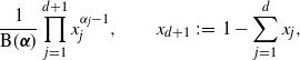 \begin{equation*}\frac1{\textrm{B}(\boldsymbol{\alpha})}\prod_{j=1}^{d+1}x_j^{\alpha_j-1},\qquad x_{d+1 }\,:\!=\, 1- \sum_{j=1}^{d}x_j,\end{equation*}
on the ‘corner’  $\Delta^{d\#} =\bigl\{{\textbf{\textit{x}}}=(x_1, \ldots, x_{d})\in \mathbb{R}^{d}_{>0}\,:\, \sum_{j=1}^{d}x_j < 1\bigr\}$. Here,
 \begin{equation*}\textrm{B}({\textbf{\textit{z}}}) \,\,:\!=\,\,\frac{\prod_{j=1}^{d+1} \Gamma (z_j)}{ \Gamma (\sum_{j=1}^{d+1}z_j)}, \qquad {\textbf{\textit{z}}}=(z_1,\ldots,z_{d+1})\in\mathbb{R}^{d+1}_{>0},\end{equation*}
is the multivariate beta function.
Keeping in mind the motivation for this work (and also for simplicity’s sake), we state our main results in a form admitting direct interpretation in terms of the dynamics of the markers in the growing tissue. We introduce the following notation for vectors of partial sums: for  ${\textbf{\textit{x}}}=(x_1,\ldots,x_k)\in \mathbb{R}^k$ we set
 $\widehat{{\textbf{\textit{x}}}}\,:\!=\,(\widehat x_1,\ldots,\widehat x_k)$, where
 $\widehat x_j=\sum_{i=1}^j x_i$,
 $j=1,\ldots, k$, and let
 $\widehat{x}_0\,:\!=\,0$. For
 $k,m\in \mathbb{N}_{>0}$ such that
 $2\le k\le m$, we set
 \begin{equation*}\Lambda_m^k \,:\!=\, \{{\textbf{\textit{x}}}\in \mathbb{N}^k_{>0}\,:\, \widehat{x}_k=m\},\qquad\Lambda_m\,:\!=\,\bigcup_{2\le k \le m}\Lambda_m^k,\qquad\Lambda \,:\!=\,\bigcup_{m \ge 2}\Lambda_m.\end{equation*}
Now recall that, in terms of the urn process (1), the locations of the d markers after  $n\ge 0$ cell divisions are
 \begin{align}M_j (n)= \widehat{\xi}_j (n),\qquad j=1,\ldots , d,\end{align}
with  $M_j (0)= N_j = \widehat{\alpha}_j$ being the initial locations of the markers given that the initial numbers of balls of different colors in the urn are specified by the vector
 $\boldsymbol{\alpha} \in \Lambda^{d+1}_N$. We set
 ${\textbf{\textit{M}}}(n)\,:\!=\, (M_1 (n), \ldots, M_{d } (n))\in\mathbb{N}^{d }_{>0}$ (recalling that we let
 $M_{d+1}(n)\,:\!=\,\widehat \xi_{d+1}(n)= N+n$,
 $n\ge 0$) and
 ${\textbf{\textit{N}}} \,:\!=\, (N_1 , \ldots, N_{d } )$.
Our first assertion is based on the Blackwell–MacQueen theorem [Reference Blackwell and MacQueen7] (closely related to the Hewitt–Savage theorem on exchangeable random variables [Reference Hewitt and Savage16]) and the strong approximation results for empirical and quantile processes. We will need some further notation. We denote by  $\{W^0(y): y\in [0,1]\}$ the standard Brownian bridge process, i.e. a continuous zero-mean Gaussian process with covariance function
 ${\mathbb E} W^0(y_1)W^0(y_2)=y_1\wedge y_2 -y_1 y_2$,
 $y_1, y_2\in [0,1]$, and by
 $\{K(y,t)\,:\, y\in [0,1], t\ge 0\}$ the (two-parameter) Kiefer process, which is a continuous zero-mean Gaussian field with covariance function
 \begin{align}{\mathbb E} K(y_1,t_1) K(y_1,t_1) = (y_1 \wedge y_2 - y_1 y_2)(t_1\wedge t_2),\qquad y_1, y_2\in [0,1], \quad t_1, t_2\ge 0.\end{align}
To help ‘visualize’ the Kiefer process, note that, for any fixed  $y\in [0,1]$, we have the equality in distribution
 $\{K(y,t)\,:\, t\ge 0 \}\stackrel{\textrm{d}}{=} \{( y(1-y))^{1/2}W(t)\,:\, t\ge 0\}$, where W is the standard Wiener process, whereas for any fixed
 $t>0$ we have
 $\{K(y,t)\,:\, y\in [0,1] \}\stackrel{\textrm{d}}{=} \{t^{1/2}W^0(y)\,:\, y\in [0,1] \}$.
Theorem 1. We can construct all the processes from the family  $\{\boldsymbol{\xi}^{\boldsymbol{\alpha}}\,:\, \boldsymbol{\alpha}\in \Lambda\} $ on a common probability space together with a sequence of Brownian bridges
 $\{ W^{0,N}\,:\, N\ge 1\}$ and a Kiefer process K independent of that sequence such that, for
 $N>d\ge 1$ and
 $n\ge 2$, for the partial sums (3) of the components of the processes
 $\boldsymbol{\xi}=\boldsymbol{\xi}^{\boldsymbol{\alpha}}$,
 $\boldsymbol{\alpha}\in \Lambda_N^{d+1}$ we have
 \begin{align} M_j (n) &= ( N + n)\widehat{\mu}_j +\frac{n}{N^{1/2}} W^{0,N} (\widehat{\mu}_j ) +\frac{n \ln N}{N } R_j\nonumber\\ &\quad + K\biggl(\widehat{\mu}_j + \frac{1}{N^{1/2}} W^{0,N} ( \widehat{\mu}_j ) +\frac{ \ln N}{N } R_j , n\biggr)+ R_j^* \ln^2 n ,\qquad j=1,\ldots, d, \end{align}
where  $ \boldsymbol{\mu} = \boldsymbol{\mu}^{ \boldsymbol{\alpha}}\,:\!=\, \boldsymbol{\alpha} / \widehat{\alpha}_{d+1}=\boldsymbol{\alpha} /N \in\Delta^d , $ and the remainder terms
 $R_j=R_j (\boldsymbol{\alpha} )$ and
 $R_j^*=R_j^* (\boldsymbol{\alpha},n)$ satisfy
 \begin{align}\limsup_{N\to\infty} \max_{1\le d
< N} \max_{\boldsymbol{\alpha}\in \Lambda^{d+1}_N} \max_{1\le j\le d} |R_j | \le C , \end{align}
 \begin{align} \limsup_{n\to \infty}\sup_{N\ge 2} \max_{1\le d
< N} \max_{\boldsymbol{\alpha}\in {\Lambda}^{d+1}_N} \max_{1\le j\le d} |R_j^* | \le C \end{align}
a.s. for some absolute constant  $C<\infty$.
The first term on the right-hand side of (5) represents the mean growth of the tissue along its longitudinal axis (which is linear in the ‘cell-division counter time’ n, but exponential in ‘real time’). The random part of the approximation on the right-hand side of (5) has different dominating terms depending on the relationship between the initial tissue length N and the number n of cell divisions. Corollary 1 presents our findings concerning the functional limit theorems for the urn processes and covers the whole spectrum of possible limiting behaviors. To state it, for  $\boldsymbol{\alpha}\in \Lambda_N^{d+1}$ we introduce the
 $(d\times d)$ matrix
 $\Sigma^{\boldsymbol{\alpha}} \,:\!=\, \bigl(\widehat{\mu}_i \wedge \widehat{\mu}_j - \widehat{\mu}_i\widehat{\mu}_j\,:\, 1\le i,j\le d\bigr)$, where
 $\boldsymbol{\mu} = \boldsymbol{\mu}^{ \boldsymbol{\alpha}}$.
Corollary 1. We can construct all the processes from the family  $\{\boldsymbol{\xi}^{\boldsymbol\alpha}\,:\, \boldsymbol{\alpha}\in \Lambda\} $ on a common probability space together with a family of multivariate Brownian motion processes
 $\{{\textbf{\textit{W}}}^{\boldsymbol{\alpha}} \,:\break \boldsymbol{\alpha}\in \Lambda \} $ with zero drift and respective covariance matrices
 $\Sigma^{\boldsymbol{\alpha}}$, and a family of Gaussian random vectors
 $\{ {\textbf{\textit{Z}}}^{\boldsymbol{\alpha}} \,:\, \boldsymbol{\alpha}\in \Lambda \} $ that are independent of these Brownian motion processes and have zero mean and the same respective covariance matrices
 $\Sigma^{\boldsymbol{\alpha}}$, such that, for the partial sums (3) for the processes
 $\boldsymbol{\xi}=\boldsymbol{\xi}^{\boldsymbol{\alpha}}$,
 $\boldsymbol{\alpha}\in \Lambda_N^{d+1}$, we have the following approximations as
 $n,N\to\infty$:
(i) if
 $n=o(N)$ then $n^{-1/2} ({\textbf{\textit{M}}} \bigl( \lfloor nt\rfloor) - (N + n t ) \widehat{\boldsymbol{\mu}}^{\#} \bigr) = {\textbf{\textit{W}}}^{\boldsymbol{\alpha}} (t) +o_P(1)$, where the error term is uniform in $t\in [0,1]$ and $\boldsymbol{\alpha}\in \Lambda_{N} $;
(ii) if
$n/N\to \nu\in \mathbb{R}_{>0}$ then $n^{-1/2} \bigl({\textbf{\textit{M}}}(\lfloor nt\rfloor) -(N + n t)\widehat{\boldsymbol{\mu}}^{\#} \bigr) = \nu^{1/2} t{\textbf{\textit{Z}}}^{\boldsymbol{\alpha}}+ {\textbf{\textit{W}}}^{\boldsymbol{\alpha}} (t) +o_P(1)$, where, for any fixed $0<a<b<\infty$, the error term is uniform in $t\in [0,1]$, $\boldsymbol{\alpha}\in \Lambda_{N} $, and $\nu\in (a,b)$;(iii) if
$N=o(n)$ then $N^{1/2}n^{-1} \bigl({\textbf{\textit{M}}} ( \lfloor nt\rfloor) -(N + n t ) \widehat{\boldsymbol{\mu}}^{\#} \bigr) = t{\textbf{\textit{Z}}}^{\boldsymbol{\alpha}} + o_P(1)$, where the error term is uniform in $t\in [0,1] $ and $\boldsymbol{\alpha}\in \Lambda_{N} $.











Restating the above results in terms of the Pólya urn processes  $\boldsymbol{\xi}(n)$ is a straightforward task.
We will now comment on the above assertions. The uniformity of the  $o_P(1)$ terms is understood in the following sense: if
 ${\textbf{\textit{R}}}(\boldsymbol{\alpha})\in\mathbb{R}^d$ is the remainder term in the respective representation for the partial sums of the process
 $\boldsymbol{\xi}^{\boldsymbol{\alpha}}$,
 $\boldsymbol{\alpha}\in \Lambda_N^{d+1}$, then, for any fixed
 $\varepsilon >0$,
 \begin{equation*}{\mathbb P} \Bigl(\max_{1\le d
< N}\max_{\boldsymbol{\alpha}\in \Lambda_N^{d+1}} \max_{1\le j\le d}|R_j(\boldsymbol{\alpha})|>\varepsilon \Bigr)\to 0\qquad\mbox{as } N\to\infty.\end{equation*}
We stress that the approximations from the corollary hold for the whole family of processes  $\boldsymbol{\xi}^{\boldsymbol{\alpha}}$ rather than for a fixed value of d.
Further, if  $n=o(N)$ (part (i)) then the dominating term on the right-hand side of (5) is the one with the Kiefer process. As the first arguments in K will be very close to the ratios
 $N_j/N=\widehat{\mu}_j$, for any initial urn composition vector
 $\boldsymbol{\alpha}\in \Lambda^{d+1}_N$ the trajectory
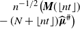 $n^{-1/2} \bigl({\textbf{\textit{M}}} (\lfloor nt\rfloor )\break - (N+ \lfloor nt\rfloor ) \widehat{\boldsymbol{\mu}}^{\#}\bigr)$,
 $t\in [0,1]$, is approximated by
 ${\textbf{\textit{W}}}^{\boldsymbol{\alpha}} (t)\,:\!=\,(K(\widehat{\mu}_1,t), \ldots, K(\widehat{\mu}_d,t))$, which is a d-dimensional Brownian motion with the specified covariance matrix
 $\Sigma^{\boldsymbol{\alpha}}.$ This is so because, at that time scale, the proportions
 $\xi_j (\lfloor nt\rfloor )/(N+\lfloor nt\rfloor)=(1+o(1)) \alpha_j /N$ of balls of different colors j in the urn vary very little when
 $t\in [0,1]$. Therefore, the dynamics of
 $\boldsymbol{\xi} (n)$ (and hence of
 ${\textbf{\textit{M}}} (n)$) is close to that of a multivariate random walk with independent and identically distributed (i.i.d.) jumps.
When n grows at the same rate as N (part (ii)), the second and fourth terms on the right-hand side of (5) are of the same magnitude. This is a transitional regime. When  $n\gg N$ (part (iii)) the Brownian bridge term is the main one. In this case, the (almost Gaussian) randomness of the limiting Dirichlet-distributed vector
 ${\textbf{\textit{V}}}$ (resulting in a random trend with an almost Gaussian coefficient for the dynamics of
 ${\textbf{\textit{M}}} (\lfloor nt\rfloor)$) dominates the random zero-mean ‘Brownian oscillations’ as the time values are very large.
Our second main result provides an upper bound for the convergence rate in the central limit theorem for the vector  ${\textbf{\textit{M}}}(n)$ of the marked agents’ location after n steps. For
 $k\ge 1$, denote by
 $\mathscr{C}^k $ the class of all Borel convex subsets of
 $\mathbb{R}^k$. For a non-negative definite symmetric matrix
 $\Sigma\in\mathbb{R}^{k\times k}$, we denote by
 $\Phi_\Sigma$ the zero-mean Gaussian distribution on
 $\mathbb{R}^k$ with covariance matrix
 $\Sigma$.
Theorem 2. Let  $d\in \mathbb{N}_{>0}$ and
 $\delta \in (0,1/(d+1))$ be fixed numbers. For any
 $N>d$,
 $n\ge 1$, and
 $\boldsymbol{\alpha}\in\Lambda_N^{d+1}$ such that
 $\alpha_j\ge \delta N$,
 $j=1,\ldots, d+1$,
 \begin{equation*} \sup_{A\in \mathscr{C}^{d}} \biggl|{\mathbb P} \biggl(\frac{{\textbf{\textit{M}}} (n) - (N+n)\widehat{\boldsymbol{\mu}}^{\#} }{((N+n) n/N)^{1/2} }\in A\biggr) -\Phi_{ \Sigma^{\boldsymbol{\alpha}}} (A)\biggr| \le c(n^{-1/2}+N^{-1/2} ). \end{equation*}
Here and in what follows, by the letter c (possibly with a subscript) we denote constants that may depend on  $\delta$ and d only and may be different even within the same formula.
Observe that the scaling used in the statement of Theorem 2 is universal: it works in all the cases (i)–(iii) in Corollary 1.
Remark 1. Note that one can also state the assertion of Theorem 2 in an equivalent form in terms of the Pólya urn composition vectors. For  $\boldsymbol{\xi} = \boldsymbol{\xi}^{\boldsymbol{\alpha}}$,
 $\boldsymbol{\mu} = \boldsymbol{\mu}^{\boldsymbol{\alpha}}$, set
 \begin{align} \boldsymbol{\Xi}(n)\,:\!=\, n^{-1/2}(\boldsymbol{\xi}^{\#}(n)- (N+ n)\boldsymbol{\mu}^{\#}), \qquad n\ge 1, \end{align}
and, for  ${\textbf{\textit{x}}}\in\mathbb{R}^k$, introduce matrices
 \begin{align} \Sigma_{\textbf{\textit{x}}}\,:\!=\,\mbox{diag} ({\textbf{\textit{x}}}) - {\textbf{\textit{x}}}^\top {\textbf{\textit{x}}}\in \mathbb{R}^{k\times k} , \end{align}
where  $\mbox{diag}\, ({\textbf{\textit{x}}})$ is the diagonal matrix with diagonal entries
 $x_j$,
 $j=1,\ldots, k$, and
 $^\top$ denotes transposition. Then, under the assumptions of Theorem 2, we equivalently have
 $\sup_{A\in \mathscr{C}^{d}}\bigl|{\mathbb P} (\boldsymbol{\Xi} (n)\in A) -\Phi_{(1+n/N)\Sigma_{\boldsymbol{\mu}^{\#}}} (A)\bigr| \le c(n^{-1/2}+N^{-1/2} )$. It will actually be more convenient for us to prove this latter bound.
2. Proofs
2.1. Proof of Theorem 1
Consider a Pólya urn process  $\boldsymbol{\xi}=\boldsymbol{\xi}^{\boldsymbol{\alpha}}$,
 $\boldsymbol{\alpha}\in \Lambda_N^{d+1}$,
 $N>d\ge 1$. It is well known that the indicator random vectors
 $\boldsymbol{\eta}(n)\,:\!=\, \boldsymbol{\xi}(n)- \boldsymbol{\xi}(n-1)$,
 $n \ge 1$, are exchangeable. By the main theorem in [Reference Blackwell and MacQueen7], given the random vector
 ${\textbf{\textit{V}}}={\textbf{\textit{V}}}^{\boldsymbol{\alpha}}$ from (2), the vectors
 $\boldsymbol{\eta}(n) $ are conditionally i.i.d.,
 \begin{align}{\mathbb P} (\boldsymbol{\eta}(1)= {\textbf{\textit{w}}}(j) \mid {\textbf{\textit{V}}})= V_j, \qquad j=1,\ldots, d+1,\end{align}
where  ${\textbf{\textit{w}}}(j)=(\delta_{j1}, \delta_{j2},\ldots, \delta_{j,d+1})$ are the respective unit coordinate vectors in
 $\mathbb{R}^{d+1}$ (here
 $\delta_{jk}$ is the Kronecker delta). Therefore, without loss of generality, one can assume that the sequence
 $\{\boldsymbol{\eta}(n)\,:\,n\ge 1\}$ is given as follows. For
 $\textbf{\textit{v}}\in \Delta^d$ and
 $u\in [0,1]$, introduce the vector-valued function
 ${\textbf{\textit{g}}} ({\textbf{\textit{v}}},u)= (g_1 (\textbf{\textit{v}},u), \ldots, g_{d+1} (\textbf{\textit{v}},u))$ as
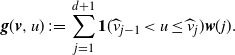 \begin{align}{\textbf{\textit{g}}} (\textbf{\textit{v}},u)\,:\!=\,\sum_{j=1}^{d+1}\textbf{1} (\widehat{v}_{j-1}
< u\le \widehat{v}_{j }){\textbf{\textit{w}}}(j).\end{align}
Assuming that  $\{U_n\,:\,n\ge 1\}$ is a sequence of i.i.d. (0,1)-uniform random variables, independent of a given random vector
 ${\textbf{\textit{V}}}\sim \textrm{Dir}_{d+1} (\boldsymbol{\alpha})$, we set
 $\boldsymbol{\eta}(n)\,:\!=\, {\textbf{\textit{g}}} ({\textbf{\textit{V}}}, U_n)$,
 $n\ge 1$. This sequence clearly satisfies (10) and is conditionally i.i.d. given the value of
 ${\textbf{\textit{V}}}$.
Now, recalling that  $\boldsymbol{\mu} = {\mathbb E} {\textbf{\textit{V}}}= \boldsymbol{\alpha}/N$, so that
 $\widehat \mu_j=N_j/N$, we have
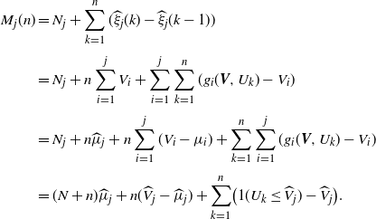 \begin{align}M_j (n) & = N_j + \sum_{k=1}^n (\widehat\xi_j (k) - \widehat{\xi}_j(k-1))\notag\\[3pt]&= N_j+ n \sum_{i=1}^j V_i + \sum_{i=1}^j \sum_{k=1}^n (g_i ({\textbf{\textit{V}}}, U_k) - V_i)\notag\\[3pt]&= N_j + n \widehat{\mu}_j + n \sum_{i=1}^j (V_i- \mu_i)+ \sum_{k=1}^n \sum_{i=1}^j (g_i ({\textbf{\textit{V}}}, U_k) - V_i)\notag\\[3pt]&= (N + n) \widehat{\mu}_j + n (\widehat{V}_j -\widehat{\mu}_j)+ \sum_{k=1}^n \bigl( {1} (U_k\le \widehat{V}_j) - \widehat{V}_j\bigr).\end{align}
The second term in the last line of (12) can be approximated using the following lemma.
Lemma 1. Let  $ \{{\textbf{\textit{X}}}^{\boldsymbol{\alpha}}\,:\, \boldsymbol{\alpha}\in \Lambda \}$ be a family of random vectors such that
 ${\textbf{\textit{X}}}^{\boldsymbol{\alpha}}\sim \textrm{Dir}_{k } (\boldsymbol{\alpha })$ for
 $\boldsymbol{\alpha}\in \Lambda_m^k$,
 $m\ge k\ge 2$. We can construct random vectors from that family on a common probability space together with a sequence of Brownian bridges
 $\{ W^{0,m}\,:\, m\ge 1\}$ such that
 \begin{align} \widehat{X}_j^{\boldsymbol{\alpha}}= \widehat{\alpha}_j /m + m^{-1/2} W^{0,m} (\widehat{\alpha}_j /m) + R ( m, \widehat{\alpha}_j ), \qquad j=1,\ldots, k, \quad \boldsymbol{\alpha}\in \Lambda_m^k, \end{align}
where
 \begin{align} \limsup_{m\to\infty} \frac{m }{\ln m} \max_{2\le k \le m}\max_{\boldsymbol{\alpha}\in \Lambda^k_m} \max_{1\le j\le k} |R (m, \widehat{\alpha}_j )|\le C\quad a.s. \end{align}
for some absolute constant  $C<\infty$.
Clearly, from (13) we also have the following representation for the original Dirichlet-distributed random vectors: for  $j=1,\ldots, k$,
 \begin{equation*}{X}_j^{\boldsymbol{\alpha}}= {\alpha}_j /m + m^{-1/2} ( W^{0,m} (\widehat{\alpha}_j /m)- W^{0,m} (\widehat{\alpha}_{j-1} /m)) + R _j ( m, \widehat{\alpha}_j )-R _j ( m, \widehat{\alpha}_{j-1} ).\end{equation*}
Proof of Lemma 1. Let  $\{U'_l\,:\, l\ge 1\}$ be a sequence of i.i.d. (0,1)-uniform random variables. Fix
 $m\ge k\ge 2$ for the moment and denote by
 $U'_{1\,:\,m-1}\le U'_{2\,:\,m-1}\le\cdots \le U'_{m-1\,:\,m-1}$ the order statistics for the sample
 $\{U'_l\,:\, 1\le l< m \}$. Set
 $U'_{0\,:\,m-1}\,:\!=\,0$,
 $U'_{m\,:\,m-1}\,:\!=\,1$. Due to the well-known fact that, for any
 ${\alpha}\in \Lambda^k_m$, we have (see, e.g., [Reference Balakrishnan and Rao3])
 \begin{equation} (U'_{ \widehat \alpha_1\,:\,m-1}-U'_{ \widehat \alpha_0 \,:\,m-1}, U'_{ \widehat \alpha_2\,:\,m-1}- U'_{\widehat \alpha_1\,:\,m-1 },\ldots, U'_{\widehat\alpha_k\,:\,m-1}- U'_{\widehat\alpha_{k-1}\,:\,m-1}) \sim \textrm{Dir}_{k } (\boldsymbol{\alpha }), \end{equation}
we can assume without loss of generality that  $\widehat{{\textbf{\textit{X}}}}{}^{\boldsymbol{\alpha}} = (U'_{\widehat\alpha_1\,:\,m-1},\ldots, U'_{\widehat\alpha_k\,:\,m-1}) $ for all
 $\boldsymbol{\alpha}\in \Lambda^k_m$ (recall also that
 $\widehat \alpha_k=m$ for such
 $\boldsymbol{\alpha}$).
Next, recall that the quantile process for our uniform sample  $\{U'_l\,:\, 1\le l< m \}$ is defined [Reference Csörgö and Révész10] as
 \begin{equation*} q_{m-1}(u)\,:\!=\, (m-1)^{1/2} \Biggl( \sum_{i=1}^{m-1} U'_{i\,:\,m-1} {1} \biggl( \frac{i-1}{m-1} <u\le\frac{i }{m-1} \biggr)-u\Biggr), \qquad u\in [0,1]. \end{equation*}
It is easily seen that
 \begin{align} m^{1/2}(\widehat{X}_j^{\boldsymbol{\alpha}}- \widehat{\alpha}_j /m) & = (1-m^{-1})^{-1/2} q_{m-1}(\widehat{\alpha}_j/ m) , \qquad j=1, \ldots, k-1 \end{align}
(note that for  $j=k$ the value of the quantity on the left-hand side of the above formula is 0). Now recall the strong approximation theorem for uniform quantile processes
 $q_{m-1}$ (see, e.g., Theorem B and Remark 1 in [Reference Csörgö and Révész10]) according to which we can construct our sequence
 $\{U'_l\,:\, l\ge 1\}$ and a sequence of Brownian bridges
 $\{ W^{0,m}\,:\, m\ge 1\}$ on a common probability space such that, for some constant
 $C<\infty$,
 \begin{align} \limsup_{m\to\infty} \frac{m^{1/2}}{\ln m} \sup_{0<u<1} |q_{m-1}(u) -W^{0,m}(u)| \le C \quad\mbox{a.s.} \end{align}
The desired assertion in (13) and (14) immediately follows from (16), (17), and the observation that the effect of the factor  $(1-m^{-1})^{-1}$ in (16) is negligible. The latter fact is a consequence of the standard exponential bound for the Brownian bridge process:
 \begin{align} {\mathbb P} \Bigl(\max_{y\in [0,1]}|W^{0}(y) |>x \Bigr) \le 2 e^{-2 x^2},\qquad x>0 \end{align}
(see, e.g., Section 9 in [Reference Billingsley4]). Indeed, combined with the Borel–Cantelli lemma, this bound implies that, for any sequence  $\{W^{0,m}\,:\, m\ge 1\}$ of Brownian bridges on a common probability space,
 \begin{align} \sum_{m=1}^\infty {1} \Bigl(\max_{y\in [0,1]}|W^{0,m}(y) |> \ln ^{1/2} m\Bigr) <\infty\qquad \textrm{a.s.} \end{align}
This, in turn, implies that the additional additive approximation error caused by the abovementioned factor in (16) is a.s.  $O(m^{-1}\ln ^{1/2} m)$. Lemma 1 is proved.
Remark 2. In the case of a fixed k and a sequence  $\boldsymbol{\alpha}(m)\in \Lambda^k_m$,
 $m\ge k$, satisfying the condition
 $\max_{1\le j\le k-1}m^{-1/2} |\widehat \alpha_j (m) - r_j m|\to 0$ for fixed
 $0<r_1< \cdots< r_{k-1}<1$, the asymptotic normality of
 $ \widehat{{\textbf{\textit{X}}}}{}^{\boldsymbol{\alpha}(m)}$ as
 $m\to \infty$ follows from Theorem 2 in [Reference Walker28]. The case of growing
 $k=k(m)\le m$ was considered under the condition that
 $k(m)/\min_{1\le j\le k(m)}\alpha_j(m)\to 0 $ as
 $m\to\infty$ in [Reference Ikeda and Matsunawa17]. It was proved in Theorem 3.1 of that paper that, for a sequence
 $\boldsymbol{\alpha}(m)\in \Lambda^{k(m)}_m$,
 $m\ge 2$, the total variation distance between the distribution of
 $\widehat{{\textbf{\textit{X}}}}{}^{\boldsymbol{\alpha}(m)}$ and the normal distribution in
 $\mathbb{R}^{k(m)}$ with the matching mean vector and covariance matrix tends to zero as
 $m\to\infty$. Upper bounds for the rate of this convergence were obtained in [Reference Matsunawa25]. The strong approximation result stated in our Lemma 1 shows that the asymptotic normality holds uniformly and without any additional assumptions on
 $\boldsymbol{\alpha}$.
Returning to the proof of Theorem 1, since  ${\textbf{\textit{V}}}\sim \mbox{Dir}_{d+1}(\boldsymbol{\alpha})$, by Lemma 1 (where we choose
 $m=N$,
 $k=d+1 $), for a suitably constructed family
 $\{{\textbf{\textit{V}}}= {\textbf{\textit{V}}}^{\boldsymbol{\alpha}}\,:\, \boldsymbol{\alpha}\in \boldsymbol{\Lambda}\}$ and sequence of Brownian bridges
 $\{W^{0,N}\,:\,N\ge 1\}$, as
 $N\to\infty$ we have
 \begin{align}\widehat{V}_j -\widehat{\mu}_j = N^{-1/2} W^{0,N} (\widehat{\mu}_j)+ O (N^{-1 }\ln N)\quad \textrm{a.s.},\end{align}
where the O-term is understood in the sense of (14).
Further, denoting by  $F_n^*(y)\,:\!=\, n^{-1}\sum_{l=1}^n \textbf{1} (U_l\le y) $ the empirical distribution function for the sample
 $\{U_l\,:\, 1\le l \le n\}$, we see that the last term on the right-hand side of (12) is equal to
 $ \phi_n (\widehat{V}_j)$, where
 $\phi_n (y) \,:\!=\,n ( F_n^* (y )- y)$,
 $y\in [0,1]$. By the Komlós–Major–Tusnády theorem [Reference Komlos, Major and Tusnady21] (see also Theorem A and Remark 1 in [Reference Csörgö and Révész10]), we can construct the sequence
 $\{ U_n\}$ on a common probability space with a Kiefer process K such that
 \begin{align}\phi_n (y) = K(y,n) + R^*(y,n), \qquad y\in [0,1], \quad n\ge 1,\end{align}
where for the remainder term  $R^*$ we have
 \begin{equation*}\limsup_{n\to \infty}\sup_{y\in [0,1]} \frac{|R^*(y,n)|}{\ln^2 n}
< C^* \quad \textrm{a.s.}\end{equation*}
for some absolute constant  $C^*<\infty$. Combining now (12), (20), and (21) (where we substitute the expression for
 $\widehat{V}_j $ from (20)) completes the proof of Theorem 1.
2.2. Proof of Corollary 1
It follows from (5) that, for  $k=1,\ldots, n$,
 \begin{align} n^{-1/2} (M_j (k) - (N+ k)\widehat{\mu}_j) = & \frac{k}{n}\biggl(\frac{n}N\biggr)^{1/2} W^{0,N} (\widehat\mu_j)+R_j kn^{-1/2}N^{-1}\ln N\nonumber\\[3pt]
& +n^{-1/2}K \bigl(\widehat{\mu}_j +\theta_{\widehat{\mu}_j,N} , k \bigr)+ R_j^* n^{-1/2}\ln^2 k,\end{align}
where, in view of (19) and (6), with probability 1,
 \begin{align}\max_{1\le d <N}\max_{\boldsymbol{\alpha}\in \Lambda_N^{d+1}}\max_{1\le j\le d}|\theta_{\widehat{\mu}_j,N}|\le 2 N^{-1/2}\ln^{1/2}N \quad \mbox{ for all sufficiently large \textit{N}.}\end{align}
(i) If
$n=o(N)$ then the first term on the right-hand side of (22) is clearly $ o_P(1)$ in view of (18). The second and fourth terms are vanishing a.s. in view of the bounds (6) and (7).For the third term on the right-hand side of (22), setting
$h_n\,:\!=\, n^{-1/3}$ and observing that $ N^{-1/2}\ln^{1/2}N =o(h_n)$, we see from (23) that, a.s. for all sufficiently large N, we have, for all $k\ge 1$,
(24)Set
\begin{align}|K(\widehat{\mu}_j + \theta_{\widehat{\mu}_j,N}, k)- K (\widehat{\mu}_j,k ) |\le\sup_{0\le u<v\le u+h_n \le 1}|K(u, k)- K (v,k ) |.\end{align}
$\beta_n\,:\!=\,(2n h_n |\ln h_n|)^{-1/2}= n^{-1/3}\bigl(\frac23 \ln n\bigr)^{-1/2}.$ Since clearly $|\ln h_n| \gg \ln\ln n$ as $n\to\infty,$ by Theorem 1.15.2 in [Reference Csörgö and Révész11] we have
Hence, the maximum of the right-hand side of (24) over
\begin{equation*}\lim_{n\to \infty} \beta_n\sup_{0\le u<v\le u+h_n \le 1}|K(u, n)- K (v,n ) |=1 \qquad \textrm{a.s.}\end{equation*}
$k=1,\ldots,n$ will be a.s. bounded by $n^{1/3}$ for all sufficiently large n. Therefore, replacing in (22) the term $ n^{-1/2}K (\widehat{\mu}_j +\theta_{\widehat{\mu}_j,N}, k )$ with $ n^{-1/2}K (\widehat{\mu}_j , k )$ will introduce an error that will uniformly be o(1) a.s.
It remains to notice that
(25)which is obvious from (4), and that
\begin{align}\{ n^{-1/2}K(y, n t)\,:\, y\in [0,1], t\ge 0\}\stackrel{\textrm{d}}{=} \{K(y, t)\,:\, y\in [0,1],t\ge 0\}, \qquad n\ge 1 ,\end{align}
$\{(K(\widehat\mu_1, t),\ldots , K(\widehat\mu_d, t))\,:\, t\ge 0\} \stackrel{\textrm{d}}{=} \{{\textbf{\textit{W}}}^{\boldsymbol{\alpha}} (t) \,:\, t\ge 0\}$ since both processes are continuous zero-mean Gaussian with a common covariance structure. That the claimed approximation holds for points t that are not multiples of $1/n$ and is uniform follows from the continuity of the approximating processes.
(ii) Here we assume that
$n/N\to \nu\in \mathbb{R}_{>0}$. The only difference in the proof from part (i) is what happens to the first term on the right-hand side of (22). For $k= \lfloor nt \rfloor$, it is now equal to $(1+o(1))t\nu^{1/2} W^{0,N} (\widehat\mu_j)$, where clearly $\bigl(W^{0,N} (\widehat\mu_1), \ldots, W^{0,N} (\widehat\mu_d)\bigr)\stackrel{\textrm{d}}{=} {\textbf{\textit{Z}}}^{\boldsymbol{\alpha}}$. Finally, we have to recall that the processes $W^{0,N}$ and K were independent of each other, which implies that ${\textbf{\textit{Z}}}^{\boldsymbol{\alpha}}$ and ${\textbf{\textit{W}}}^{\boldsymbol \alpha}$ in our approximation are also independent.(iii) Applying the scaling used in the case when
$N=o(n)$, (22) turns into
For
\begin{align*}N^{ 1/2}n^{-1 } (N_j (k) - (N+ k)\widehat{\mu}_j)& =\frac{k}n W^{0,N} (\widehat\mu_j)+R_j \frac{k}n N^{-1/2}\ln N\notag\\& \quad +\biggl(\frac{N}n\biggr)^{1/2}n^{-1/2}K \bigl(\widehat{\mu}_j +\theta_N , k \bigr)+ R_j^*\biggl(\frac{N}n\biggr)^{1/2} \frac{\ln^2 k}{n^{1/2}}.\end{align*}
$k=\lfloor nt\rfloor$, the first term on the right-hand side is $(1+o(1) )t W^{0,N} (\widehat\mu_j)$, yielding the approximating term $t{\textbf{\textit{Z}}}^{\boldsymbol{\alpha}}$. The second and fourth terms are vanishing a.s. due to the bounds (6) and (7). Finally, it follows from (25) and (18) that the third term on the right-hand side is $o_P(1)$. The corollary is proved.



























2.3. Proof of Theorem 2
Using the notation from (8), we will start by rewriting the representation in (12) as
 \begin{align}\boldsymbol{\Xi}(n) = n^{1/2} ({\textbf{\textit{V}}}^{\#} - \boldsymbol{\mu}^{\#}) +{\textbf{\textit{Y}}} ({\textbf{\textit{V}}},n),\end{align}
where, recalling the notation in (11), we set  ${\textbf{\textit{Y}}}({\textbf{\textit{v}}},n)\,:\!=\, n^{-1/2}\sum_{k=1}^n \boldsymbol{\gamma}({\textbf{\textit{v}}}, k)$ and
 $\boldsymbol{\gamma}({\textbf{\textit{v}}}, k) \,:\!=\, {\textbf{\textit{g}}}^{\#} ({\textbf{\textit{v}}}, U_k) - {\textbf{\textit{v}}}^{\#}$,
 ${\textbf{\textit{v}}}\in \Delta^{d}$,
 $k\ge 1$. As could be expected from Corollary 1, it will turn out that the two terms on the right-hand side of (26) are asymptotically independent and normal, with a common correlation matrix.
It follows from (26) that, for any  $A\in \mathscr{C}^d $,
 \begin{align}{\mathbb P} \bigl(\boldsymbol{\Xi}(n)\in A\bigr)= \int_{\Delta^d}{\mathbb P} \bigl( {\textbf{\textit{Y}}} ({\textbf{\textit{v}}},n) \in A- n^{1/2} ({\textbf{\textit{v}}}^{\#} - \boldsymbol{\mu}^{\#}) \bigr){\mathbb P} ({\textbf{\textit{V}}} \in \textrm{d}{\textbf{\textit{v}}} ).\end{align}
The rest of the proof will consist of the following steps. First, we will show that, up to a uniform additive error term  $O(n^{-1/2}+N^{-1/2})$, the integrand here equals
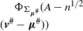 $\Phi_{\Sigma_{\boldsymbol{\mu}^{\#}}} ( A - n^{1/2}\break ({\textbf{\textit{v}}}^{\#} - \boldsymbol{\mu}^{\#}))$ (recall that
 $\Sigma_{\textbf{\textit{x}}} $ was defined in (9)). With the integrand replaced by this expression, the integral on the right-hand side of (27) is just the value on the set A of the convolution of
 $\Phi_{\Sigma_{\boldsymbol{\mu}^{\#}}}$ with the distribution of
 ${\textbf{\textit{V}}}^{\#}-\boldsymbol{\mu}^{\#}$. To complete the argument, we will apply a known result on the convergence rate in total variation of the joint distribution of sample quantiles (which coincides with the distribution of
 $\widehat{{\textbf{\textit{V}}}}^{\#}$) to the respective Gaussian law.
It is easily seen that, for any  ${\textbf{\textit{v}}}\in \Delta^d$, the random vectors
 $\boldsymbol{\gamma} ({\textbf{\textit{v}}} ,k)$,
 $k\ge 1$, are i.i.d.,
 ${\mathbb E} \boldsymbol{\gamma} ({\textbf{\textit{v}}} ,1)= {0}$,
 $\textrm{Cov}\, (\boldsymbol{\gamma} ({\textbf{\textit{v}}} ,1))=\Sigma_{{\textbf{\textit{v}}}^{\#}}$. Therefore, from a multivariate version of the Berry–Esseen bound (see, e.g., relation (1) in [Reference Sazonov27]) we conclude that, for some constant
 $c<\infty$ that depends on d only,
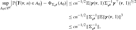 \begin{align}\sup_{A_0\in\mathscr{C}^{d} }\bigl|{\mathbb P} \bigl( {\textbf{\textit{Y}}} ({\textbf{\textit{v}}},n) \in A_0 \bigr) - \Phi_{\Sigma_{{\textbf{\textit{v}}}^{\#}}} (A_0 )\bigr|& \le c n^{-1/2}{\mathbb E}|\boldsymbol{\gamma} ({\textbf{\textit{v}}} ,1)\Sigma^{-1}_{{\textbf{\textit{v}}}^{\#}}\boldsymbol{\gamma}^\top ({\textbf{\textit{v}}} ,1)|^{3/2}\notag \\[3pt]& \le c n^{-1/2}\|\Sigma^{-1}_{{\textbf{\textit{v}}}^{\#}}\| {\mathbb E}\|\boldsymbol{\gamma} ({\textbf{\textit{v}}} ,1)\|^3 \notag \\[3pt] & \le c n^{-1/2}\|\Sigma^{-1}_{{\textbf{\textit{v}}}^{\#}}\| ,\end{align}
since clearly  $\|\boldsymbol{\gamma} ({\textbf{\textit{v}}} ,1)\| \le 2$. We can easily verify by direct computation that, setting
 ${\textbf{\textit{e}}}\,:\!=\,(1,\ldots, 1)\in \mathbb{R}^d$,
 \begin{align}\Sigma^{-1}_{{\textbf{\textit{u}}}} = \mbox{diag}({\textbf{\textit{u}}}^{-1}) +\frac{{\textbf{\textit{e}}}^\top {\textbf{\textit{e}}}}{1-\widehat{{\textbf{\textit{u}}}}_d},\qquad {\textbf{\textit{u}}}\in \Delta^{d\#}.\end{align}
So, for the matrix operator norm in (28) we get
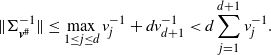 \begin{align}\|\Sigma^{-1}_{{\textbf{\textit{v}}}^{\#}}\|\le\max_{1\le j\le d } v_j^{-1} + dv_{d+1}^{-1}<d\sum_{j=1}^{d+1} v_j^{-1}.\end{align}
Now we will bound the difference between  $\Phi_{\Sigma_{{\textbf{\textit{v}}}^{\#}}} (A_0 )$ and
 $\Phi_{\Sigma_{\boldsymbol{\mu}^{\#}}} (A_0 )$. For random vectors
 ${\textbf{\textit{Y}}}'\sim P'$,
 ${\textbf{\textit{Y}}}''\sim P''$ taking values in
 $\mathbb{R}^k$,
 $k\ge 1$, denote by
 \begin{align}d_\textrm{TV}({\textbf{\textit{Y}}}',{\textbf{\textit{Y}}}'')= d_\textrm{TV}(P',P'')\,:\!=\,\sup_B |P'( B)-P''( B)|\equiv \sup_g |{\mathbb E} g ({\textbf{\textit{Y}}}' ) - {\mathbb E} g ({\textbf{\textit{Y}}}'')|\end{align}
the total variation distance between the distributions of these vectors (the first supremum is taken over all Borel  $B\subset \mathbb{R}^k$, the second one over all measurable functions
 $g\,:\,\mathbb{R}^k\to [0,1]$; see, e.g., Chapter 3 in [Reference Rachev, Klebanov, Stoyanov and Fabozzi26]). For a matrix
 $\mathcal{A}= (a_{ij}\,:\, 1\le i,j\le k)\in\mathbb{R}^{k\times k}$, denote by
 $\|\mathcal{A}\|_\textrm{F}\,:\!=\,\bigl( \sum_{i,j=1}^k a_{ij}^2\bigr)^{1/2}$ its Frobenius norm. By Theorem 1.1 in [Reference Devroye, Mehrabian and Reddad13],
 \begin{align}d_\textrm{TV} (\Phi_{\Sigma_{{\textbf{\textit{v}}}^{ \#}} }, \Phi_{\Sigma_{\boldsymbol{\mu}^{ \#}} } )\le2 \|\Sigma_{\boldsymbol{\mu}^{ \#}} ^{-1}\Sigma_{{\textbf{\textit{v}}}^{ \#}} -\mathcal{I}_d\|_\textrm{F}\le2 \|\Sigma_{\boldsymbol{\mu}^{ \#}} ^{-1}\|_\textrm{F}\cdot \|\Sigma_{{\textbf{\textit{v}}}^{ \#}} - \Sigma_{\boldsymbol{\mu}^{ \#}} \|_\textrm{F}\end{align}
as  $\|\cdot \|_\textrm{F}$ is sub-multiplicative. From (29), under the assumptions of Theorem 2 we clearly have
 \begin{equation*}\|\Sigma^{-1}_{\boldsymbol{\mu}^{ \#}} \|_\textrm{F}^2\le2 \sum_{j=1}^d \mu_j^{-2} + 2 d^2 \mu_{d+1}^{-2}<2d(d+1)\delta^{-2} .\end{equation*}
The last factor in (32) does not exceed  $\|\mbox{diag} ({\textbf{\textit{v}}}^{ \#})- \mbox{diag} (\boldsymbol{\mu}^{ \#}) \|_\textrm{F}+\| ({\textbf{\textit{v}}}^{ \#})^\top {\textbf{\textit{v}}}^{ \#}- (\boldsymbol{\mu}^{ \#})^\top \boldsymbol{\mu}^{ \#} \|_\textrm{F}$, where the square of the first term is
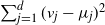 $\sum_{j=1}^d (v_j-\mu_j)^2 $, whereas that of the second one is
 \begin{align*}\sum_{i,j=1}^d (v_i v_j-\mu_i \mu_j)^2\le2\sum_{i,j=1}^d v_i^2( v_j- \mu_j)^2+ 2\sum_{i,j=1}^d \mu_j^2( v_i- \mu_i)^2\le 4 \sum_{j=1}^d (v_j-\mu_j)^2 .\end{align*}
Thus, we have from (32) the bound  $d_\textrm{TV} (\Phi_{\Sigma_{{\textbf{\textit{v}}}^{ \#}} }, \Phi_{\Sigma_{\boldsymbol{\mu}^{ \#}} } )\le c\|{\textbf{\textit{v}}}-\boldsymbol{\mu}\|$.
Combining this with (28) and (30) yields
 \begin{align}\sup_{A_0\in \mathscr{C}^{d} }\bigl|{\mathbb P} \bigl( {\textbf{\textit{Y}}} ({\textbf{\textit{v}}},n) \in A_0 \bigr) - \Phi_{\Sigma_{\boldsymbol{\mu}^{ \#}} }(A_0 )\bigr|\le c R_n ({\textbf{\textit{v}}},\boldsymbol{\mu}),\end{align}
where  $R_n ({\textbf{\textit{v}}},\boldsymbol{\mu})\,:\!=\,n^{-1/2} \sum_{j=1}^{d+1} v_j^{-1 } + \|{\textbf{\textit{v}}} -\boldsymbol{\mu} \|$. To use this bound in (27), we need to compute the expectation of
 $ R_n ({\textbf{\textit{V}}},\boldsymbol{\mu})$. First note that since
 ${\textbf{\textit{V}}}\sim \mbox{Dir}_{d+1}(\boldsymbol{\alpha})$, the components
 $V_j$ of this vector are beta-distributed with respective parameters
 $( \alpha_j, N - \alpha_j)$,
 $j=1,\ldots, d+1$. Hence,
 \begin{align*}{\mathbb E} V_j^{-1 }= \frac{\textrm{B}( \alpha_j-1, N - \alpha_j )}{\textrm{B}(\alpha_j, N - \alpha_j)}= \frac{\Gamma(\alpha_j-1)\Gamma(N )}{\Gamma(N -1)\Gamma(\alpha_j )}=\frac{N-1}{\alpha_j-1}
< \frac2{\delta}\end{align*}
as, in view of the assumption that  $\alpha_j\ge \delta N$, we can assume without loss of generality that
 $\alpha_j\ge 2$. As the variance of the beta distribution with parameters
 $a, b>0$ equals
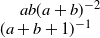 $ab (a+b)^{-2}\break (a+b+1)^{-1}$, we get
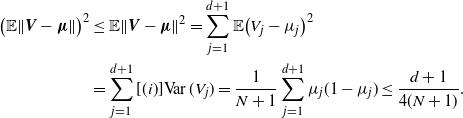 \begin{align*}\bigl({\mathbb E} \|{\textbf{\textit{V}}} -\boldsymbol{\mu} \|\bigr)^2& \le {\mathbb E} \|{\textbf{\textit{V}}} -\boldsymbol{\mu} \|^2=\sum_{j=1}^{d+1}{\mathbb E} \bigl( V_j -\mu_j \bigr)^2\notag\\&=\sum_{j=1}^{d+1}[(i)]\textrm{Var}\, ( V_j)=\frac1{N+1}\sum_{j=1}^{d+1}\mu_j (1-\mu_j)\le \frac{d+1}{4(N+1)}.\end{align*}
We conclude that
 \begin{align}{\mathbb E} R_n ({\textbf{\textit{V}}},\boldsymbol{\mu}) \le c(n^{-1/2}+ N^{-1/2}) .\end{align}
Now we obtain from (27), (33), and (34) that, for  $A\in\mathscr{C}^d $,
 \begin{align}\bigl|{\mathbb P} (\boldsymbol{\Xi}(n)\in A )-{\mathbb E}\Phi_{\Sigma_{\boldsymbol{\mu}^{ \#}} }(A- n^{1/2} ({\textbf{\textit{v}}}^{\#} - \boldsymbol{\mu}^{\#})) \bigr|\le c(n^{-1/2}+ N^{-1/2}).\end{align}
It follows from (15) (with  $k=d+1$,
 $m=N$) and Theorem 3.1 in [Reference Matsunawa25] that, under the assumptions of our Theorem 2, for a random vector
 $\boldsymbol{\zeta}\sim \Phi_{\Sigma_{\boldsymbol{\mu}^{ \#}}}$,
 $d_\textrm{TV} ({\textbf{\textit{V}}}^{\#}-\boldsymbol{\mu}^{\#}, N^{-1/2}\boldsymbol{\zeta}) \le c N^{-1/2}$. Now, from (35) and the last relation in (31) we see that
 \begin{align*}\bigl|{\mathbb P} (\boldsymbol{\Xi}(n)\in A )-{\mathbb E} \Phi_{\Sigma_{\boldsymbol{\mu}^{ \#}} }\bigl(A - n^{1/2} N^{-1/2} \boldsymbol{\zeta} \bigr) \bigr|\le c(n^{-1/2}+ N^{-1/2}).\end{align*}
Since, clearly,  ${\mathbb E} \Phi_{\Sigma_{\boldsymbol{\mu}^{ \#}} }\bigl(A - n^{1/2} N^{-1/2} \boldsymbol{\zeta} \bigr) = \Phi_{(1 +n/N)\Sigma_{\boldsymbol{\mu}^{ \#}}}(A), $ Theorem 2 is proved in view of Remark 1.
Acknowledgement
The author is grateful to the anonymous referees and associate editor for their useful comments that helped him improve the exposition of the paper.


