1. INTRODUCTION
The study of stimulated Brillouin scattering (SBS) instability in laser–plasma interaction has been object of continuous theoretical and experimental research interest for decades in the context of inertial confinement fusion (ICF) scheme (Kruer, Reference Kruer1988; Aleksandrov et al., Reference Aleksandrov, Brenner, Koval'skii, Loburev and Rubenchik1985; Berger et al., Reference Berger, Lasinski, Langdon, Kaiser, Afeyan, Cohen, Still and Williams1995; Afshar-rad et al., Reference Afshar-Rad, Gizzi, Desselberger and Willi1996; Giulietti et al., Reference Giulietti, Macchi, Schifano, Biancalana, Danson, Giulietti, Gizzi and Willi1999; Gao et al., Reference Gao, Lu, Wang, He and Hasi2010). This instability occurs during the propagation of an intense laser beam through plasma in the presence of ion density fluctuations, where the incident light wave decays into an ion-acoustic wave (IAW) and a scattered electromagnetic wave (Baldis et al., Reference Baldis, Campbell and Kruer1991). There is a net energy loss in the process of stimulated Brillouin backscattering (SBBS), which is measured by the backward SBS reflectivity (Riconda et al., Reference Riconda, Heron, Pesme, Huller, Tikhonchuk and Detering2005). SBS instability grows in the plasma corona (which surrounds the fuel pellet in laser fusion experiments) resulting in a large amount of backscattered laser radiation. This radiation reduces the coupling efficiency of laser light into the plasma and destroys the high degree of symmetry necessary for efficient compression of the capsule (Lindl, Reference Lindl1995). Therefore, it is necessary to improve the ability to predict and control the growth of SBS instability under conditions relevant to the ICF scheme.
Owing to crucial importance of the SBS process in the laser-driven ICF scheme, it receives a great deal of attention both theoretically (Sodha et al., Reference Sodha, Umesh and Sharma1979; Huller, Reference Huller1991; Baldis et al., Reference Baldis, Labuane, Moody, Jalinaud and Tikhonchuk1998; Divol et al., Reference Divol, Cohen, Williams, Langdon and Lasinski2003; Huller et al., Reference Huller, Masson-Laborde, Pesme, Labaune and Bandulet2008; Singh & Walia, Reference Singh and Walia2012; Sharma & Singh, Reference Sharma and Singh2013; Masson-Laborde et al., Reference Masson-Laborde, Huller, Pesme, Labuane, Depierreux, Loiseau and Bandulet2014) and experimentally (Afshar-rad et al., Reference Afshar-Rad, Gizzi, Desselberger and Willi1996; Labaune et al., Reference Labaune, Baldis and Tikhonchuk1997; Baton et al., Reference Baton, Amiranoff, Malka, Modena, Salvati and Coulaud1998; Chirokikh et al., Reference Chirokikh, Seka, Simon, Craxton and Tikhonchuk1998; Giulietti et al., Reference Giulietti, Macchi, Schifano, Biancalana, Danson, Giulietti, Gizzi and Willi1999). The filamentation of laser beam increases the local laser intensity (high-intensity filaments) and induces the stimulated Brillouin back scattering (B-SBS) in the plasma. Giulietti et al. (Reference Giulietti, Macchi, Schifano, Biancalana, Danson, Giulietti, Gizzi and Willi1999) have experimentally described the measurements of the B-SBS from underdense expanding plasmas in a regime of strong filamentation. In this case, the overall SBS reflectivity was extremely low (10−4). The filamentary structure of SBS sources was found in the experiments described in (Afshar-rad et al., Reference Afshar-Rad, Gizzi, Desselberger and Willi1996; Labaune et al., Reference Labaune, Baldis, Schifano, Bauer, Michard, Renard, Seka, Moody and Estabrook1996). Afshar-rad et al. (Reference Afshar-Rad, Gizzi, Desselberger and Willi1996) studied an experimental study of stimulated Brillouin backscatter (B-SBS) produced in a large homogeneous underdense plasma column by an intense laser pulse (over nearly two orders of magnitude in irradiances 1013–1015 W/cm2). This study indicates that the formation of laser filaments controls the onset of B-SBS emission and supports a correlation between the suppression of B-SBS and the effectiveness of induced spatial incoherence (ISI) in suppressing filamentation. The SBS reflectivity was of the order of 10−2 which is much higher than that observed in the experiment (Giulietti et al., Reference Giulietti, Macchi, Schifano, Biancalana, Danson, Giulietti, Gizzi and Willi1999). Experimental reflectivity due to SBS and ion-acoustic fluctuations has been successfully measured (over four orders of magnitude of SBS reflectivity) in the plasma by a randomized laser beam (Labaune et al., Reference Labaune, Baldis and Tikhonchuk1997). It has also been observed that the mode coupling of the ion waves in the primary and secondary SBBS processes leads to enhanced damping of the ion waves which reduces their amplitudes and the SBBS reflectivity (Cohen et al., Reference Cohen, Baldis, Berger, Williams and Labaune1998) as observed in the L’ Utilisation des Lasers Intenses (LULI) experiments (Baldis et al., Reference Baldis, Labuane, Schifano, Renard and Michard1996).
The growth of SBS process has been investigated experimentally in various conditions such as laser smoothing and focusing, varying laser intensities, and plasma densities (Fuchs et al., Reference Fuchs, Labuane, Depierreux, Tikhonchuk and Baldis2000; Reference Fuchs, Labuane, Depierreux, Baldis, Michard and James2001). It has been observed that the SBS process gets affected in the presence of self-focused pump laser beam and ion-acoustic beam. The effect of pump depletion and self-focusing on the SBS process has been studied (Mahmoud et al., Reference Mahmoud, Sharma, Kumar and Yadav1999) and it was found that the reflectivity of SBS decreases by several orders of magnitude. The particle-in-cell simulation also shows the filament formation and its effects on the SBS process (Matsuoka et al., Reference Matsuoka, Lei, Yabuuchi, Adumi, Zheng, Kodamal, Sawai, Suzuki, Kitagawa, Norimatsu, Nagai, Nagatomo, Izawa, Mima, Sentoku and Tanaka2008). Sharma and Singh (Reference Sharma and Singh2013) have recently investigated the excitation of IAW and SBBS of the filamented hollow Gaussian beams in a collisionless plasma due to the presence of a laser beam carrying null intensity at center, and found that self-focusing and back reflectivity reduce for higher order of hollow Gaussian beams. Recently, Gauniyal et al. (Reference Gauniyal, Chauhan, Rawat and Purohit2014) investigated the effect of rippled laser beam on the excitation of IAW in the presence of relativistic–ponderomotive non-linearity.
In most of the study of SBS during past two decades, there is a vast difference found between the experimental and theoretical results (Chirokikh et al., Reference Chirokikh, Seka, Simon, Craxton and Tikhonchuk1998; Giacone & Vu, Reference Giacone and Vu1998; Maximov et al., Reference Maximov, Oppitz, Rozmus and Tikhonchuk2000; Moody et al., Reference Moody, MacGowan, Rothenberg, Berger, Divol, Glenzer, Kirkwood, Williams and Young2001). One of the main reasons is taking idealized theoretical assumptions made in the theory and saturation effects of SBS-driven IAWs. The theoretical work has been focused on the propagation of uniform transverse intensity profile of the pump beams in plasmas but in the experiment, laser beams of finite transverse size have non-uniform intensity distribution along the wave front. Such beams may modify the background plasma density, suffer filamentation (self-focusing), and affects the reflectivity of scattering instabilities. In addition, smooth Gaussian intensity profile of the laser beam has been used in the earlier studies of filamentation and SBS; however, it is experimentally observed that smooth appearing laser beam is essentially non-smooth, but comprises superimposed intensity spikes, which may lead to distortion of self-focusing in non-linear media (Abbi & Mahr, Reference Abbi and Mahr1971). Similarly, much of the previous work on filamentation and SBBS, ponderomotive and relativistic non-linearities has been separately taken into account. However, in actual case when the high-power laser beam propagates in the plasma, both relativistic and ponderomotive non-linearities are simultaneously arise depending on the time scale of the laser pulse (Brandi et al., Reference Brandi, Manus and Mainfray1993a; Kumar et al., Reference Kumar, Gupta and Sharma2006). In this case, electrons are expelled from the high-intensity region by a ponderomotive force; the non-linearity in the dielectric constant of the plasma comes by electron mass variation due to laser intensities and due to changes in the electron density on account of the ponderomotive force. Therefore, the laser beam propagation is expected to be drastically affected in comparison with only relativistic or ponderomotive cases.
Keeping above points in mind, an attempt has been made toward the analytical and numerical study of SBBS of a ring-rippled laser beam in the plasma under paraxial approximation (Akhmanov et al., Reference Akhmanov, Sukhorukov and Khokhlov1968; Sodha et al., Reference Sodha, Ghatak and Tripathi1976). All the relevant parameters have been expanded in terms of the radial distance from the maximum of the ring ripple, which is away from the axis (r = 0). The plasma is electrically neutral everywhere and the pulse duration τ (with condition τpe < τ < τpi, where τ is the laser pulse duration, τ pi is the ion plasma period, and τ pe is the electron time period) has been chosen so that both the non-linearities viz. relativistic and ponderomotive are operative. In Section 2, we have given a brief summary of the self-focusing of the main and rippled laser beam, growth of ring ripple in the plasma, and intensity of the main and ring-rippled beam in the presence of relativistic and ponderomotive non-linearities. The effect of ring ripple growth on IAW excitation and the SRBS process is presented in Sections 3 and 4, respectively. Section 5 presents numerical results and discussions. The main conclusions are summarized in Section 6.
2. ANALYTICAL FORMULATION
2.1. Propagation of Intense Laser Beam in Plasma
Consider the propagation of an intense Gaussian laser beam along the z-axis with a small coaxial perturbation superimposed on the main beam (the ring ripple) having its electric vector along the y-axis in a homogeneous plasma. The effective electric field vector E of a Gaussian beam with a coaxial ring ripple can be expressed as (Sodha et al., Reference Sodha, Sharma, Prakash and Verma2004)
 $${\bf E} = \hat j \,(E_0 + E_1 )\exp \,(i{\rm \omega} _0 t),$$
where
 $$(E_0){_{z = 0}} = \hat j \;{\displaystyle{{E_{00}} \over {\,f_0}}} \exp (- r^2 /2r_0^2 f_0^2),$$
and
 $$(E_1){_{z = 0}} = \hat j \;{\displaystyle{{E_{10}} \over {\,f_1}}} \left( {\displaystyle{{r^2} \over {r_1^2 f_1^2}} - {\rm \delta}} \right)^{n/2} \exp \left( {\displaystyle{{- r^2} \over {2r_1^2 f_1^2}}} \right)\exp (i{\rm \phi}_{\rm p} ),$$
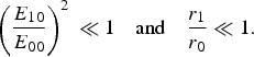
where E 00 and E 10 are the initial amplitude of the main Gaussian beam of width r 0 and the ring ripple of width r 1 with maximum  $r_{\max} = r_1 \sqrt {(n + {\rm \delta})} $ at z = 0, respectively. n and δ are positive numbers characterizing the position of the ring ripple on the wave front of the electromagnetic beam. ϕP is the initial phase difference between the electric field vector of the Gaussian beam and the ring ripple, z is the distance along the direction of propagation, r is the radial coordinate in a cylindrical coordinates system,
 $\hat j$ is a unit vector perpendicular to the z-axis, and f 0 and f 1 are the beam width parameters of the main beam and the ripple beam, respectively. The ring ripple is usually a small perturbation over the main beam and its parameters may be assumed to satisfy
 $$\left( {\displaystyle{{E_{10}} \over {E_{00}}}} \right)^2 \, \ll 1 \quad {\rm and} \quad \displaystyle{{r_1} \over {r_0}} \ll 1.$$
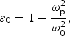
The dielectric constant of the plasma is given by
 $${\rm \varepsilon} _0 = 1 - \displaystyle{{{\rm \omega}_{\rm p}^2} \over {{\rm \omega}_0^2}},$$
where ωp is the plasma frequency given by 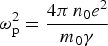 ${\rm \omega} _{\rm p}^2 = \displaystyle{{4{\rm \pi} \,n_0 e^2} \over {m_0 {\rm \gamma}}} $ (with e is the charge of an electron, m 0 its rest mass, and n 0 is the electron density of plasma electron in the absence of laser beam) and γ is the relativistic factor given by
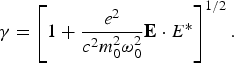 $${\rm \gamma} = \left[ {1 + \displaystyle{{e^2} \over {c^2 m_0^2 {\rm \omega}_0^2}} {\bf E} \cdot E^{\ast}} \right]^{1/2}. $$
The above expression is valid when there is no change in the plasma density. The relativistic–ponderomotive force on an electron in the presence of an intense laser beam may be represented as (Borisov et al., Reference Borisov, Borovisiky, Shiryaev, Korobkin, Prokhorov, Solem, Luk, Boyer and Rhodes1992; Brandi et al., Reference Brandi, Manus and Mainfray1993a; Reference Brandi, Manus, Mainfray, Lehner and Bonnaud1993b)
 $$F_{\rm P} = -m_0 c^2 \nabla ({\rm \gamma} - 1).$$
Using the electron continuity equation and the current density equation for the second-order correction in the electron density equation, the total density can be expressed as (Brandi et al., Reference Brandi, Manus and Mainfray1993a; Reference Brandi, Manus, Mainfray, Lehner and Bonnaud1993b)
 $$n_{\rm T} = n_0 + n_2 = n_0 + \displaystyle{{c^2 n_0} \over {{\rm \omega}_{\rm p}^2}} \left({\nabla ^2 {\rm \gamma} - \displaystyle{{(\nabla {\rm \gamma})^2} \over {\rm \gamma}}} \right),$$
where
 $$\displaystyle{{n_{\rm T}} \over {n_{0}}} = 1 + \displaystyle{{c^{2}} \over {{\rm \omega} _{\rm p}^{\rm 2} {\rm \gamma}}} \left[ { - \displaystyle{{2a} \over {r_{0}^{2}\, f_{0}^{4}}} - \displaystyle{{2r^{2} a^{2}} \over {{\rm \gamma} ^{2} r_{0}^{4}\, f_{0}^{8}}} e^{ - ({{r^{2}} / {r_{0}^{2}\, f_{0}^{2}}})} + \displaystyle{{2r^{2} a} \over {r_{0}^{4}\, f_{0}^{6}}}} \right]e^{ - ({{r^{2}} / {r_{0}^{2}\, f_{0}^{2}}})}. $$
Now the effective dielectric constant of the plasma at frequency ω0 is given by
 $${\rm \varepsilon} = {\rm \varepsilon} _0 + {\rm \phi} (E_0^{\ast} \cdot E_0^{\ast} ),$$
where
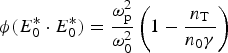 $${\rm \phi} (E_0^{\ast} \cdot E_0^{\ast}) = \displaystyle{{{\rm \omega}_{\rm p}^{\rm 2}} \over {{\rm \omega}_0^2}} \left( {1 - \displaystyle{{n_{\rm T}} \over {n_0 {\rm \gamma}}}} \right)$$
Following Akhmanov et al. (Reference Akhmanov, Sukhorukov and Khokhlov1968), the intensity and the dimensionless beam width parameter (f 0) of the main laser beam are given by the following equations (Rawat et al., Reference Rawat, Gauniyal and Purohit2014):
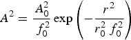 $$A^2 = {\displaystyle{{A_0^2} \over {\,f_0^2}}} \exp \left({ - \displaystyle{{r^2} \over {r_0^2\, f_0^2}}} \right)$$
and
 $$\displaystyle{{d^2}{\,f_0} \over {dz^2}} = \displaystyle{{{c^2}} \over {{{\rm \varepsilon }_{\rm f}}{\rm \omega }_0^2 r_0^4\, f_0^3 }} - \displaystyle{{{\rm \omega }_{\rm p}^{\rm 2} {\,f_0}} \over {{\rm \omega }_0^2 {{\rm \varepsilon }_{\rm f}}}}\left[ {\displaystyle{a \over {2{{\rm \gamma }^3}r_0^2\, f_0^4 }} - \displaystyle{{3a} \over {{{\rm \gamma }^2}k_{\rm p}^2 r_0^4\, f_0^6 }} - \displaystyle{{3{a^2}} \over {{{\rm \gamma }^4}k_{\rm p}^2 r_0^4\, f_0^8 }}} \right], $$
where a = αA 02 (A 02 = E 002) is square of the dimensionless vector potential and k p2 = ωp2/c 2, and rest of symbols have their usual meanings.
The intensity (A 10) and growth rate (g i) of ring ripple are given by (Rawat et al., Reference Rawat, Gauniyal and Purohit2014)
 $$A_{10}^2 = \displaystyle{{E_{10}^2} \over {\,f_1^2}} \left( {\displaystyle{{r^2} \over {r_1^2 \,f_1^2}} - {\rm \delta}} \right)^n \exp \left( { - \displaystyle{{r^2} \over {r_1^2 \,f_1^2}}} \right)\exp \left( { - 2\int_0^z {g_{\rm i} (z)}} \right),$$
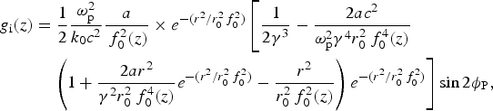 $$\eqalign{{g_{\rm i}}(z) & = \displaystyle{1 \over 2}\displaystyle{{{\rm \omega }_{\rm p}^{\rm 2} } \over {{k_0}{c^2}}}\displaystyle{a \over {\,f_0^2 (z)}} \times e^{ - ({{r^2} / {r_0^2\, f_0^2}} )} \left[\displaystyle{1 \over {2{\rm \gamma} ^3}} - \displaystyle{{2ac^2} \over {{\rm \omega} _{\rm p}^2 {\rm \gamma} ^4 r_0^2\, f_0^4 (z)}} \right. \cr & \left.\quad\left(1+ {\displaystyle{{2a{r^2}} \over {{{\rm \gamma }^{\rm 2}}r_0^2\, f_0^4 (z)}}} {{e^{ - ({{{r^2}} / {r_0^2\, f_0^2 }})}}} - {\displaystyle{{{r^2}} \over {r_0^2 \,f_0^2 (z)}}}\right){{e^{ - ({{{r^2}} / {r_0^2 \,f_0^2 }})}}}\right]\sin 2{{\rm \phi }_{\rm P}},}$$
where f 1 is the dimensionless beam width parameter of the ring ripple and is given by
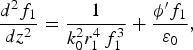 $$\displaystyle{{d^2 f_1} \over {dz^2}} = \displaystyle{1 \over {k_0^2 r_1^4 \,f_1^3}} + \displaystyle{{{\rm \phi}^{\prime} f_1} \over {{\rm \varepsilon} _0}}, $$
where
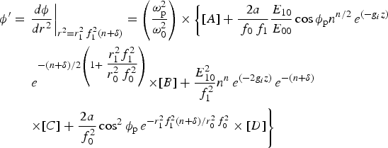 $$\eqalign{{{\rm \phi }^{\prime}} &= {\left. {\displaystyle{{d{\rm \phi }} \over {d{r^2}}}} \right\vert_{{r^2} = r_1^2 \,f_1^2 (n + {\rm \delta })}}=\left( {\displaystyle{{{\rm \omega }_{\rm p}^{\rm 2} } \over {{\rm \omega }_{\rm 0}^{\rm 2} }}} \right)\times \left\{[A] + \displaystyle{{2a} \over {{\,f_0}{\,f_1}}}\displaystyle{{{E_{10}}} \over {{E_{00}}}}\cos {{\rm \phi }_{\rm p}}{n^{n/2}}\,{e^{( - {g_i}z)}}\right.\cr &\quad\ \left. e^{{{ - (n + {\rm \delta })} / 2}\left( 1 + \displaystyle{{r_1^2 f_1^2 } \over {r_0^2 \,f_0^2 }} \right)}{ \times [B] + \displaystyle{{E_{10}^2 } \over {\,f_1^2 }}{n^n}\,e^{( - 2{g_i}z)}}\,e^{ - (n + {\rm \delta })}\right.\cr &\quad\ \left. \times [C] + \displaystyle{{2a} \over {\,f_0^2 }}\cos ^2{\rm \phi }_{\rm p}\,e^{ - r_1^2 f_1^2 (n + {\rm \delta }) / r_0^2\, f_0^2 } \times [D]\right\}} $$
with
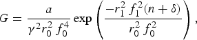 $$G = \displaystyle{a \over {{\rm \gamma}^2 r_0^2\, f_0^4}} \exp \left({\displaystyle{{ - r_1^2\, f_1^2 (n + {\rm \delta})} \over {r_0^2 \,f_0^2}}} \right),$$
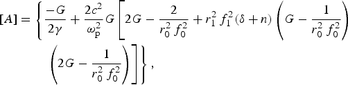 $$\eqalign{\left[A \right] &= \left\{{ \displaystyle{-G \over {2{\rm \gamma}}}} + {\displaystyle{{2c^2} \over {{\rm \omega} _{\rm p}^{\rm 2}}}} G \left[ {2G - {\displaystyle{2 \over {r_0^2 \,f_0^2}}}+ r_1^2 \,f_1^2 ({\rm \delta} + n)\left( {G -{ \displaystyle{1 \over {r_0^2\, f_0^2}}}} \right)} \right. \right. \cr & \quad \left. \left. \quad\left({2G - {\displaystyle{1 \over {r_0^2\, f_0^2}}}} \right) \right] \right\},}$$
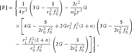 $$\hskip-25pt\eqalign{ \left[B \right] &= \left\{{ \displaystyle{1 \over {4{\rm \gamma} ^3}}} \left( {3G - {\displaystyle{1 \over {r_0^2 \,f_0^2}}}} \right) - {\displaystyle{{2c^2} \over {{\rm \omega} _{\rm p}^2 {\rm \gamma} ^2}}} G \right. \cr &\quad\ \left. \times \left[ {4G - {\displaystyle{5 \over {2r_0^2 \,f_0^2}}}+ 2Gr_1^2 \,f_1^2 ({\rm \delta} + n)\left( {3G -{ \displaystyle{5 \over {2r_0^2 \,f_0^2}}}} \right)} \right. \right. \cr & \quad\ - \left. \left.{ \displaystyle{{r_1^2\, f_1^2 ({\rm \delta} + n)} \over {r_0^2 \,f_0^2}}} \left({2G - {\displaystyle{3 \over {2r_0^2 \,f_0^2}}}} \right) \right] \right\},}$$
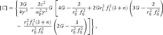 $$\hskip10pt\eqalign{\left[C \right] & = \left\{{ \displaystyle{3G \over {4{\rm \gamma} ^3}}} - {\displaystyle{{2c^2} \over {{\rm \omega} _{\rm p}^2 {\rm \gamma} ^2}}} G \right. \left. \left[ {4G - {\displaystyle{2 \over {r_0^2 \,\,f_0^2}}}+ 2Gr_1^2 \,f_1^2 ({\rm \delta} + n)\left( {3G -{ \displaystyle{2 \over {r_0^2 \,\,f_0^2}}}} \right)} \right. \right. \cr & \quad\ \ - \left. \left.{ \displaystyle{{r_1^2 f_1^2 ({\rm \delta} + n)} \over {r_0^2 \,f_0^2}}} \left({2G - {\displaystyle{1 \over {r_0^2 \,f_0^2}}}} \right) \right] \right\},}$$
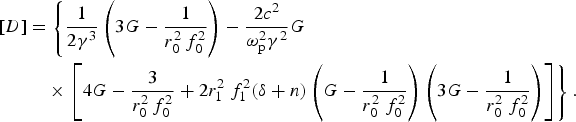 $$\hskip10pt\eqalign{\left[ D \right] &= \left\{ {\displaystyle{1 \over {2{\rm \gamma} ^3}} \left( {3G - \displaystyle{1 \over {r_0^2 \,f_0^2}}} \right) - \displaystyle{{2c^2} \over {{\rm \omega} _{\rm p}^2 {\rm \gamma} ^2}} G} \right. \cr &\quad \times \left. {\left[ {4G - \displaystyle{3 \over {r_0^2 \,f_0^2}} + 2 r_1^2\ f_1^2 ({\rm \delta} + n)\left( {G - \displaystyle{1 \over {r_0^2 \ f_0^2}}} \right)\left( {3G - \displaystyle{1 \over {r_0^2 \ f_0^2}}} \right)} \right]} \right\}.} $$
Equation (11) determines the focusing/defocusing of the ring ripple (superposed on the main Gaussian laser beam), where the first two terms on the right-hand side represent the diffraction phenomenon and the second term describes the non-linear refraction of the beam, which arises due to the relativistic–ponderomotive non-linearity.
3. EXCITATION OF ION ACOUSTIC WAVE
On account of the change in the background density due to the ponderomotive force and the relativistic effects as well as coupling between the ring-rippled laser beam and plasma, IAW is excited. To study the effects of the ring-rippled Gaussian laser beam in the presence of relativistic–ponderomotive non-linearity on the excitation of IAW in the collisionless plasma, the following set of fluid equations are used:
(1) Continuity equation
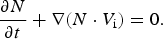
(12) $$\displaystyle{{\partial N} \over {\partial t}} + \nabla (N \cdot V_{\rm i} ) = 0.$$
(2) Momentum equation
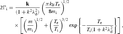
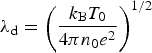
(13)where 2Γe is the Landau damping factor given by Krall and Trivelpicec (Reference Krall and Trivelpicec1973)$$\eqalign{m_{\rm i} \left[ {\displaystyle{{\partial V_{\rm i}} \over {\partial t}} + (V_{\rm i}. \nabla)} \right] = eE + \displaystyle{e \over c}(V_{\rm i} \times B) - 2\Gamma _{\rm i} m_{\rm i} V_{\rm i} - \displaystyle{{{\rm \gamma} _{\rm i} \nabla P} \over N}},$$where$$\eqalign{2\Gamma _{\rm i} & = \displaystyle{{\bf k} \over {(1 + k^2 {\rm \lambda} _{\rm d}^2 )}}\left( {\displaystyle{{\pi k_{\rm B} T_{\rm e}} \over {8m_{\rm i}}}} \right)^{\!\!1/2} \cr &\quad \times \left[ {\left( {\displaystyle{m \over {m_{\rm i}}}} \right)^{\!\!1/2} + \left( {\displaystyle{{T_{\rm e}} \over {T_{\rm i}}}} \right)^{\!\!3/2} \exp \left\{ { - \displaystyle{{T_{\rm e}} \over {T_{\rm i} (1 + k^2 {\rm \lambda} _{\rm d}^2}}} \right\}} \right],}$$${\rm \lambda} _{\rm d} = \left( {\displaystyle{{k_{\rm B} T_0} \over {4{\rm \pi} n_0 e^2}}} \right)^{1/2} $ is the Debye length and k is the wave vector of the acoustic wave. T e and T i are the electron and ion temperatures, and V i is the ion fluid density.(3) Poisson's equation
(14)$$\nabla \cdot E_{{\rm si}} = - 4{\rm \pi} e(n_{{\rm es}} - n_{{\rm is}} ),$$where n es and n is correspond to perturbations in the electron and ion densities, and are related to each other by the following equation:
(15)$$n_{{\rm es}} = \displaystyle{{n_{{\rm is}}} \over {\left[ {1 + ({{k^2 {\rm \lambda} _{\rm d}^2} / {(n_{\rm T} /n_0 {\rm \gamma} )}})} \right]}}.$$



Applying the perturbation approximation, N = n 0 + n is, V i = v is, and E = E H + E si, where n is ≪ N 0 and using Eqs. (12)–(15), one obtains the general equation governing the ion density variation
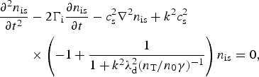 $$\eqalign{\displaystyle{{\partial ^2 n_{{\rm is}}} \over {\partial t^2}}& - 2\Gamma _{\rm i} \displaystyle{{\partial n_{{\rm is}}} \over {\partial t}} - c_{\rm s}^{\rm 2} \nabla ^2 n_{{\rm is}} + k^2 c_{\rm s}^2 \cr & \times \left( { - 1 + \displaystyle{1 \over {1 + k^2 {\rm \lambda} _{\rm d}^2 (n_{\rm T} /n_0 {\rm \gamma} )^{ - 1}}}} \right)n_{{\rm is}} = 0,}$$
where c s = (k BT e/M)1/2 is the speed of IAW for T e ≫ T i.
The solution of Eq. (16) can be written as
 $$n_{{\rm is}} = n_1 (r,z)\exp \{ i[{\rm \omega} t - k(z + S(r,z))]\}. $$
Here n 1 is the slowly varying real function of r and z, ω and k are the frequency and propagation constant, and S is the eikonal for IAW. The frequency and wave number of the IAW satisfy the following dispersion relation in the presence of laser beam
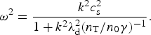 $${\rm \omega} ^2 = \displaystyle{{k^2 c_{\rm s}^{\rm 2}} \over {1 + k^2 {\rm \lambda}_{\rm d}^2 (n_{\rm T} /n_0 {\rm \gamma} )^{-1}}}. $$
Substituting Eq. (17) into (16) and separating the real and imaginary parts, one obtains the real part as
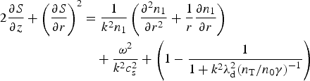 $$\eqalign{2{\displaystyle{{\partial S} \over {\partial z}}} + {\left( {\displaystyle{{\partial S} \over {\partial r}}} \right)^2} & = {\displaystyle{1 \over {{k^2}{n_1}}}}\left( {\displaystyle{{{\partial ^2}{n_1}} \over {\partial {r^2}}} + \displaystyle{1 \over r}\displaystyle{{\partial {n_1}} \over {\partial r}}} \right) \cr &\quad + \displaystyle{{{{\rm \omega }^2}} \over {{k^2}c_{\rm s}^2 }} + \left( {1 - \displaystyle{1 \over {1 + {k^2}{\rm \lambda }_{\rm d}^{\rm 2} {{({n_{\rm T}}/{n_0}{\rm \gamma })}^{ - 1}}}}} \right) }$$
and
 $${\displaystyle{{\partial n_1^2} \over {\partial z}}} + \left( {\displaystyle{1 \over r}\displaystyle{{\partial S} \over {\partial r}} + {\displaystyle{{{\partial ^2}S} \over {\partial {r^2}}}}} \right)n_1^2 + {\displaystyle{{\partial n_1^2 } \over {\partial r}}\displaystyle{{\partial S} \over {\partial r}}} + \displaystyle{{2{\Gamma _{\rm i}}{\rm \omega }} \over {kc_{\rm s}^2 }}n_1^2 = 0. $$
To solved the couple Eqs. (19a) and (19b), we assume the initial radial variation of IAW density perturbation to be Gaussian and the solution at finite z may be written as
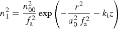 $$n_1^2 = \displaystyle{{n_{00}^2} \over {\,f_{\rm a}^2}} \exp \left( { - \displaystyle{{r^2} \over {a_0^2 \,f_{\rm a}^2}} - k_{\rm i} z} \right) $$
and
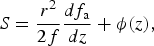 $$S = \displaystyle{{r^2} \over {2f}}\displaystyle{{df_{\rm a}} \over {dz}} + {\rm \phi} (z), $$
where k i = Γiω/kc s2, is the damping factor, f a is a dimensionless beam width parameter, and a 0 is the initial beam width of acoustic wave. We have used the following boundary conditions df a/dz = 0, f = 1 at z = 0. Using Eqs. (20a) and (20b) in Eq. (19a) and equating the coefficients of r 2 on both sides, we obtain the following equation governing:
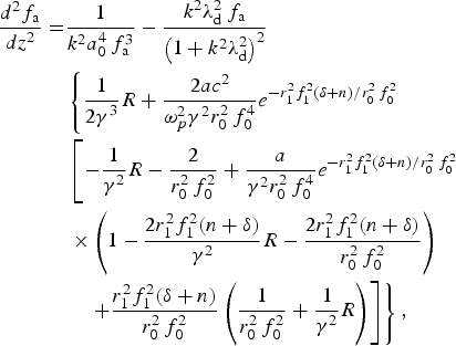 $$\eqalign{\displaystyle{{d^2 f_{\rm a}} \over {dz^2}} = & \displaystyle{1 \over {k^2 {a_0^4} \,f_{\rm a}^3}} -\displaystyle{{k^2 {\rm \lambda} _{\rm d}^{\rm 2} \,f_{\rm a}} \over {\left( {1 + k^2 {\rm \lambda} _{\rm d}^2} \right)^2}} \cr & \left\{ \displaystyle{{1} \over {2{\rm \gamma}}^3}R + \displaystyle{{2ac^2} \over {{\rm \omega}_p^2 {\rm \gamma}^2 r_0^2 \,f_0^4 }}e^{ - r_1^2 f_1^2 (\delta + n)/r_0^2 \,f_0^2} \right. \cr &\left. \left[\displaystyle{- {{1} \over {{\rm \gamma}}^2}R} - \displaystyle{2 \over {r_0^2 \,f_0^2}} + \displaystyle{a \over {{\rm \gamma} ^2 r_0^2 \,f_0^4}} e^{ - r_1^2 f_1^2 (\delta + n)/r_0^2 \,f_0^2} \right. \right. \cr & \left. \left. \times \left( {1 - \displaystyle{{{{2r_1^2}f_1^2 (n + {\rm \delta})} \over {\rm \gamma}^2}}R - \displaystyle{{2r_1^2}f_1^2 (n + {\rm \delta}) \over {r_0^2 \,f_0^2}}} \right)\right. \right. \cr &\quad \left.\left. + \displaystyle{{r_1^2 f_1^2 ({\rm \delta} + n)} \over {r_0^2 \,f_0^2}} \left( {\displaystyle{1 \over {r_0^2 \,f_0^2}} + \displaystyle{1 \over {{\rm \gamma} ^2}} R} \right) \right] \right\},} $$
where
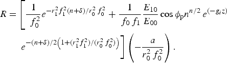 $$\eqalign{&{R} = \left[{\displaystyle{1 \over {\,\,f_0^2}} }e^{ - r_1^2 f_1^2 (n + {\rm \delta} )/r_0^2 \,f_0^2} + \displaystyle{1 \over {{\,f_0}{\,f_1}}}\displaystyle{{{E_{10}}} \over {{E_{00}}}}\cos {{\rm \phi }_{\rm p}}{n^{n/2}}\,{e^{( - {g_i}z)}}\right.\cr &\qquad \left. e^{{{ - (n + {\rm \delta })} / 2}\left( 1 + ({r_1^2 f_1^2}) / ({r_0^2 \,f_0^2}) \right)}\right]\left( - \displaystyle{a \over {r_0^2 \,f_0^2}}\right).}$$
The modified value of γ is
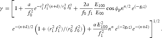 $$\eqalign{{\rm \gamma} &= \left[{\displaystyle{{1} + {a \over {\,\,f_0^2}}} }e^{ - r_1^2 f_1^2 (n + {\rm \delta} )/r_0^2 \,f_0^2} + \displaystyle{2a \over {{\,f_0}{\,f_1}}}\displaystyle{{{E_{100}}} \over {{E_{00}}}}\cos {{\rm \phi }_{\rm p}}{n^{n/2}}\,{e^{( - {g_i}z)}}\right.\cr &\quad\ \left. e^{{ - (n + {\rm \delta })} / 2}\left( 1 + ({r_1^2 f_1^2}) / ({r_0^2 \,f_0^2}) \right) + \displaystyle{{{\rm \alpha}E_{100}^2 } \over {\,f_1^2 }}{n^n}\,e^{( - 2{g_i}z)}e^{ - (n + {\rm \delta })}\right]^{1/2}.} $$
Equation (21) describes the beam width parameter (f a) of the excited IAW in the collisionless plasma with df a/dz = 0, and f a = 1 at z = 0.
4. STIMULATED BRILLOUIN SCATTERING
Consider a high-electric field ET which is the sum of the electric field of the pump laser beam with a coaxial ring ripple (E = E 0 + E 1) and the electric field of scattered wave E S
 $${\bf E}_{\rm T} = {\bf E}\exp \,(i{\rm \omega} _0 t) + E_{\rm S} (i{\rm \omega} _{\rm S} t),$$
where ω0 and ωS are the frequency of the incident laser beam and scattered beam. The vector ET satisfy the wave equation
 $$\nabla ^2 {\bf E}_{\rm T} - \nabla (\nabla \cdot {\bf E}_{\rm T} ) = \displaystyle{1 \over {c^2}} \displaystyle{{\partial ^2 {\bf E}_{\rm T}} \over {\partial t^2}} + \displaystyle{{4{\rm \pi}} \over {c^2}} \displaystyle{{\partial {\bf J}_{\rm T}} \over {\partial t}}, $$
where JT is the current density vector in the presence of high-frequency electric vector ET. Equating the terms at scattered frequency E S, one gets
 $$\nabla ^2 E_{\rm S} + \displaystyle{{{\rm \omega} _{\rm S}^{\rm 2}} \over {c^2}} \left[ {1 - \displaystyle{{n_{\rm T}} \over {n_0}} \displaystyle{{{\rm \omega} _{\rm p}^2} \over {{\rm \gamma \omega} _{\rm S}^{\rm 2}}}} \right]E_{\rm S} = \displaystyle{1 \over 2}\displaystyle{{{\rm \omega} _{\rm P}^2} \over {c^2}} \displaystyle{{{\rm \omega} _{\rm S}} \over {{\rm \omega} _{\rm 0}}} \displaystyle{{n^\ast} \over {n_0}} {\bf E}. $$
In solving Eq. (23b) the term ∇(∇·E S) may be neglected in comparison with the ∇2·E S term. Let the solution of (23b)
 $$E_{\rm S} = E_{{\rm S}0} (r,z)\exp \,(ik_{{\rm S}0} z) + E_{{\rm S}1} (r,z)\exp \,( - ik_{{\rm S}1} z),$$
where
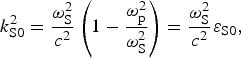 $$k_{{\rm S0}}^{\rm 2} = \displaystyle{{{\rm \omega} _{\rm S}^{\rm 2}} \over {c^2}} \left( {1 - \displaystyle{{{\rm \omega} _{\rm p}^2} \over {{\rm \omega} _{\rm S}^{\rm 2}}}} \right) = \displaystyle{{{\rm \omega} _{\rm S}^{\rm 2}} \over {c^2}} {\rm \varepsilon} _{{\rm S}0}, $$
k S1 and ωS satisfy the phase-matching conditions ωS = ω0 − ω and k S1 = k 0 − k. Here E S0 and E S1 are slowly varying real functions of r and z, and k S1 and k S0 are the propagation constants of the scattered wave. Using Eq. (24) in (23a) and (23b) and separating terms with different phases we obtain
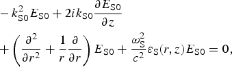 $$\eqalign{&-k_{{\rm S}0}^2 {E_{{\rm S}0}} + 2i{k_{{\rm S0}}}\displaystyle{{\partial {E_{{\rm S}0}}} \over {\partial z}} \cr & + \left( {\displaystyle{{{\partial ^2}} \over {\partial {r^2}}} + \displaystyle{1 \over r}\displaystyle{\partial \over {\partial r}}} \right){E_{{\rm S}0}} + \displaystyle{{{\rm \omega }_{\rm S}^{\rm 2} } \over {{c^2}}}{{\rm \varepsilon }_{\rm S}}(r,z){E_{{\rm S}0}} = 0,} $$
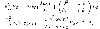 $$\eqalign{& - k_{{\rm S1}}^{\rm 2} {E_{{\rm S}1}} - 2i{k_{{\rm S}1}}\displaystyle{{\partial {E_{{\rm S}1}}} \over {\partial z}} + \left( {\displaystyle{{{\partial ^2}} \over {\partial {r^2}}} + \displaystyle{1 \over r}\displaystyle{\partial \over {\partial r}}} \right){E_{{\rm S}1}} \cr & + \displaystyle{{{\rm \omega }_{\rm S}^{\rm 2} } \over {{c^2}}}{{\rm \varepsilon }_{\rm S}}(r,z){E_{{\rm S1}}} = \displaystyle{1 \over 2}\displaystyle{{{\rm \omega }_{\rm p}^{\rm 2} } \over {{c^2}}}\displaystyle{{{{\rm \omega }_{\rm S}}} \over {{{\rm \omega }_0}}}\displaystyle{{n^\ast} \over {{n_0}}}{E_0}\,{e^{ - i{k_0}{S_0}}},} $$
where
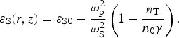 $${\rm \varepsilon} _{\rm S} (r,z) = {\rm \varepsilon} _{{\rm S0}} - \displaystyle{{{\rm \omega} _{\rm p}^{\rm 2}} \over {{\rm \omega} _{\rm S}^{\rm 2}}} \left( {1 - \displaystyle{{n_{\rm T}} \over {n_0 {\rm \gamma}}}} \right).$$
Now the solution for Eq. (27) may be written as
 $$E_{{\rm S}1} = E_{{\rm S}1}^{\prime} (r,z)\exp ( - ik_0 S_0 ).$$
Substituting Eq. (28) into (27) and neglecting terms containing space derivatives, one obtains the following equation:
 $$E_{{\rm S1}}^{\rm ^{\prime}} \cong - \displaystyle{1 \over 2}\displaystyle{{{\rm \omega} _{\rm p}^{\rm 2}} \over {c^2}} \displaystyle{{n^{\ast}} \over {n_0}} \displaystyle{{{\rm \omega} _{\rm S}} \over {{\rm \omega} _0}} \displaystyle{{\hat EE_0} \over {\left[ {k_{{\rm S1}}^{\rm 2} - k_{{\rm S}0}^2 - ({{{\rm \omega} _{\rm p}^{\rm 2}} / {c^2}} )\left( {1 - ({{n_{\rm T}} / {n_0 {\rm \gamma}}} )} \right)} \right]}}, $$
where  $\hat E$ is a unit vector along E.
By putting E S0 = E S00(r,z) exp (ik S0S c) in Eq. (26) and separating the real and imaginary parts, one can obtain
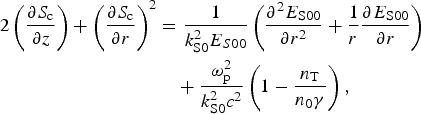 $$\eqalign{2\left( {\displaystyle{{\partial {S_{\rm c}}} \over {\partial z}}} \right) + {\left( {\displaystyle{{\partial {S_{\rm c}}} \over {\partial r}}} \right)^2} & = \displaystyle{1 \over {k_{{\rm S0}}^{\rm 2} {E_{S00}}}}\left( {\displaystyle{{{\partial ^2}{E_{{\rm S}00}}} \over {\partial {r^2}}} + \displaystyle{1 \over r}\displaystyle{{\partial {E_{{\rm S}00}}} \over {\partial r}}} \right) \cr &\quad + \displaystyle{{{\rm \omega }_{\rm p}^{\rm 2} } \over {k_{{\rm S}0}^2 {c^2}}}\left( {1 - \displaystyle{{{n_{\rm T}}} \over {{n_0}{\rm \gamma }}}} \right),} $$
 $$\displaystyle{{\partial E_{{\rm S00}}^{\rm 2}} \over {\partial z}} + \displaystyle{{\partial E_{{\rm S00}}^{\rm 2}} \over {\partial r^2}} \displaystyle{{\partial S_{\rm c}} \over {\partial r}} + \left( {\displaystyle{{\partial ^2 S_{\rm c}} \over {\partial r^2}} + \displaystyle{1 \over r}\displaystyle{{\partial S_{\rm c}} \over {\partial r}}} \right)E_{{\rm S}00}^2 = 0. $$
Here E S00 is the real function of r and z and S c is the eikonal for the scattered wave. Solution of Eqs. (30a) and (30b) can be written as
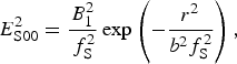 $$E_{{\rm S00}}^{\rm 2} = \displaystyle{{B_1^2} \over {\,f_{\rm S}^2}} \exp \left( { - \displaystyle{{r^2} \over {b^2 f_{\rm S}^2}}} \right),$$
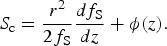 $$S_{\rm c} = \displaystyle{{r^2} \over {2f_{\rm S}}} \displaystyle{{df_{\rm S}} \over {dz}} + {\rm \phi} (z).$$
Here B 1 is the amplitude of the scattered beam, whose value is to be determined by boundary conditions. f s is the dimensionless beam width parameters of the scattered beam and satisfy the following differential equation:
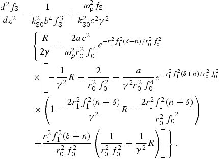 $$\eqalign{\displaystyle{{d^2 f_{\rm S}} \over {dz^2}} = & \displaystyle{1 \over {k_{{\rm S}0}^2 b^4 f_{\rm S}^3}} + \displaystyle{{{\rm \omega} _{\rm p}^{\rm 2} f_{\rm S}} \over {k_{{\rm S}0}^2 c^2 {\rm \gamma} ^2}} \cr & \left\{ \displaystyle{{R} \over {2{\rm \gamma}}} + \displaystyle{{2ac^2} \over {{\rm \omega}_p^2 r_0^2 \,f_0^4 }}e^{ - r_1^2 f_1^2 (\delta + n)/r_0^2 \,f_0^2} \right. \cr &\left. \times \left[\displaystyle{- {{1} \over {\rm \gamma}^2}R} - \displaystyle{2 \over {r_0^2 \,f_0^2}} + \displaystyle{a \over {{\rm \gamma} ^2 r_0^2 \,f_0^4}} e^{ - r_1^2 f_1^2 (\delta + n)/r_0^2 \,f_0^2} \right. \right. \cr & \left. \left. \times \left( {1 - \displaystyle{{{{2r_1^2}f_1^2 (n + {\rm \delta})} \over {\rm \gamma}^2}}R - \displaystyle{{2r_1^2}f_1^2 (n + {\rm \delta}) \over {r_0^2 \,f_0}^2}} \right)\right. \right. \cr &\left.\left. + \displaystyle{{r_1^2 f_1^2 ({\rm \delta} + n)} \over {r_0^2 \,f_0^2}} \left( {\displaystyle{1 \over {r_0^2 \,f_0^2}} + \displaystyle{1 \over {{\rm \gamma} ^2}} R} \right) \right] \right\}.} $$
5. BACK REFLECTIVITY
Now the value of B 1 may be obtained on applying appropriate boundary conditions at z = z c
 $$E_{\rm S} = E_{{\rm S}0} (r,z)\,e^{{\rm ik}_{{\rm S0}} z} + E_{{\rm S}1} (r,z)\,e^{ - ik_{S1} z} = 0,$$
where z c = L − z and L is the interaction length. Here z c is chosen sufficiently large, so that n 00 is nearly zero.
Therefore, at z = z c one gets
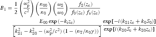 $$\eqalign{ {B_1} & = \displaystyle{1 \over 2}\left( {\displaystyle{{{\rm \omega }_{\rm p}^{\rm 2} } \over {{c^2}}}} \right)\left( {\displaystyle{{{n_{00}}} \over {{n_0}}}} \right)\left( {\displaystyle{{{{\rm \omega }_{\rm S}}} \over {{{\rm \omega }_0}}}} \right)\displaystyle{{{\,f_{\rm S}}({z_{\rm c}})} \over {{\,f_0}({z_{\rm c}}){\,f_{\rm a}}({z_{\rm c}})}} \cr & \quad \displaystyle{{{E_{00}}\exp \,( - {k_{\rm i}}{z_{\rm c}})} \over {\left[ {k_{{\rm S}1}^2 - k_{{\rm S0}}^{\rm 2} - ({{{\rm \omega }_{\rm p}^2 } / {{c^2}}})\left( {1 - ({{{n_{\rm T}}} / {{n_0}{\rm \gamma }}})} \right)} \right]}}\displaystyle{{\exp \,[ - i({k_{{\rm S}1}}{z_{\rm c}} + {k_0}{S_0})]} \over {\exp \,[i({k_{{\rm S}0}}{S_{\rm c}} + {k_{{\rm S}0}}{z_{\rm c}})]}}} $$
with condition
 $$\displaystyle{1 \over {b^2 f_{\rm S}^2}} = \displaystyle{1 \over {r_0^2 \,f_0^2}} + \displaystyle{1 \over {a_0^2 \,f_{\rm a}^{\rm 2}}}. $$
Here f S(z c) and f a(z c) are the values of dimensionless beam width parameter of scattered beam and electron plasma beam at z = z c.
Back reflectivity is defined as the ratio of backscattered power to the incident power and is given by
 $$\eqalign{R \cong & \displaystyle{1 \over 4}\left( {\displaystyle{{{\rm \omega} _{\rm p}^{\rm 2}} \over {c^2}}} \right)^2 \left( {\displaystyle{{n_{00}} \over {n_0}}} \right)^2 \left( {\displaystyle{{{\rm \omega} _{\rm S}} \over {{\rm \omega} _0}}} \right)^2\cr &\quad \displaystyle{1 \over {\left[ {k_{{\rm S}1}^2 - k_{{\rm S}0}^2 - ({{{\rm \omega} _{\rm p}^{\rm 2}} / {c^2}} )\left( {1 - ({{n_{\rm T}} / {n_0 {\rm \gamma}}} )} \right)} \right]^2}} \times \displaystyle{{E_{00}^2} \over {(E_{00}^2 + E_{10}^2 )}} \cr & \times \left\{ \displaystyle{{\,f_{\rm s}^2 (z_{\rm c} )} \over {\,\,f_0^2 (z_{\rm c} )\, f_{\rm a}^2 (z_{\rm c} )\, f_{\rm s}^2 (z)}} \exp \left( { - 2k_{\rm i} z_{\rm c} - \displaystyle{{r^2} \over {b^2 f_{\rm s}^2}}} \right)\right.\cr & \left. + \displaystyle{1 \over {\,\,f_0^2 (z)\, f_{\rm a}^2 (z)}}\exp \left( { - 2k_{\rm i} z - \displaystyle{{r^2} \over {r_0^2 \,f_0^2}} - \displaystyle{{r^2} \over {a_0^2 \,f_{\rm a}^2}}} \right)\right. \cr &\left. - \displaystyle{{2f_{\rm S} (z_{\rm c} )} \over {\,f_0 (z_{\rm c} ) f_{\rm a} (z_{\rm c} )\,f_0 (z)f_{\rm a} (z)\,f_{\rm S} (z)}}\right. \cr &\quad \left. \exp \left( { - k_{\rm i} z_{\rm c} - k_{\rm i} z - \displaystyle{{r^2} \over {2r_0^2 \,f_0^2}} - \displaystyle{{r^2} \over {2a_0^2 \,f_{\rm a}^{\rm 2}}} - \displaystyle{{r^2} \over {2b^2 f_{\rm s}^2}}} \right)\right.\cr &\quad \left. \cos \,(k_{{\rm s}0} + k_{{\rm s}1} )(z_{\rm c} - z) \right\}.} $$
6. RESULTS AND DISCUSSION
Numerical computations have been performed to obtain the appreciable results due to the propagation of ring ripple superimposed on the main laser beam in terms of the variations of the intensities of the main laser beam, ring rippled beam, IAW, and the back reflectivity of SBS with the propagation distance. To have a numerical evaluation of the relativistic–ponderomotive self-focusing and to evaluate the effect of the change of the parameters of the plasma and the laser beams in the paraxial region, we have performed the numerical computation of Eqs. (7), (9), (20a), and (36). These coupled equations have been solved and the numerical results obtained for the well-established typical plasma and laser beam parameters. The following set of the parameters has been used in the numerical calculation:
 $$\eqalign{&{{\rm \omega }_0} = 1.77 \times 10^{15}\;{\rm rad/s},\quad r{_0} = 20\,\mu {\rm m},\quad {r_1} = 0.8{r_0},\cr & {E_{10}} = 0.01{E_{00}},\quad {v_{{\rm th}}}^2 = 0.1c,\; \quad \; 2{\,\phi_{\rm p}} = {\rm \pi }/2,\,\;{\rm and}\;{\rm \delta } = n = 1,}$$
and the initial boundary conditions for both f 0 and f 1 are
 $$\displaystyle{{df_0} \over {dz}} = \displaystyle{{df_1} \over {dz}} = 0\quad {\rm and}\quad f_0 = f_1 = 0\quad {\rm at}\quad z = 0.$$
The intensity profiles of the main laser beam and ring ripple are expressed by Eqs. (7) and (9) respectively when relativistic and ponderomotive non-linearities are operative. Equations (8) and (11) describe the beam width of the main laser beam (f 0) and ring ripple beam (f 1), which determine the focusing/defocusing behavior of both beams respectively along the distance of propagation in the plasma. The intensity profile of both beams depends on the beam width parameter f 0 and f 1. In both equations [Eqs. (8) and (11)], the first term on the right-hand side represents the diffraction phenomena and the second term describes the non-linear refraction of the beam in the presence of both relativistic and ponderomotive non-linearities. The relative magnitude of these two terms determines the focusing and defocusing behavior of the beams.
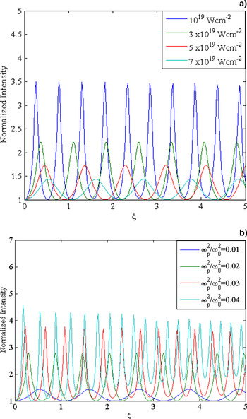
Figures 1a and 1b show the intensity profile of the main laser beam in the plasma with the normalized distance of propagation. The laser beam gets filamented due to the laser plasma coupling. When a laser beam propagates through the plasma, then the density of the plasma will vary through the channel due to ponderomotive force; however, intensity profile of the main laser beam modified significantly because the relativistic and ponderomotive non-linearities introduced in the plasma depend on the total intensity of the beam. Figure 1a clearly shows, as the initial laser beam intensity (αE 002) increases, the normalized laser beam intensity in the plasma with normalized distance of propagation decreases. It is obvious from Figure 1b that with the increase in the plasma density at constant αE 002, the normalized intensity of the laser beam starts increasing due to the complex dependency of beam width parameter (f 0) on plasma density.
(a) Variation in normalized intensity of main laser beam in plasma with normalized distance (ξ = zc/ω0r 02) for constant ω p2/ω02(=0.2) and for different laser beam intensities. (b) Variation in normalized intensity of the main laser beam in plasma with normalized distance (ξ = zc/ω0r 02) for constant laser intensity (a = 3 × 10¹⁹ W/cm2) and for different plasma frequencies, when both relativistic and ponderomotive non-linearities are operative.

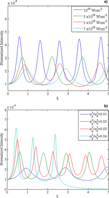
The intensity profile of ring ripple depends on the growth rate of ring ripple in the plasma and the beam width parameter (f 1) of the ring-rippled beam. Equations (9), (10), and (11) respectively expressed the axial intensity and growth rate of ring ripple in the plasma and beam width parameter (f 1) of the ring-rippled beam. It is apparent from Eqs. (8) and (11) due to coupling between the main beam and the ring ripple, the ring ripple can grow/decay in the plasma. The growth rate (g i) of the ring ripple depends on the effective intensity of the main beam in the plasma, electron density in the plasma, frequency of the laser beam, phase angle ϕp, and the parameters n and δ. It has been observed that the ripple grows only when sin ϕp is negative in Eq. (10). Figures 2a and 2b present the variation of the axial intensity of ring ripple in the plasma with the distance of propagation for different values of laser intensities and plasma frequencies, respectively. It is obvious that the patterns of the intensity profile of ring ripple are same as the main laser beam, but there is a vast difference of intensity, that is, the intensity of ring ripple gets suppressed by a factor of 10−4. This is due to the complex dependency of beam width parameters of the main and ring-rippled laser beam on ripple intensity. The intensity of ring-like spikes on the main laser beam significantly affected IAW generation and the SBBS process in the plasma. It is also important to mention here that the parameters ϕp, n, and δ also affected the profile of the axial intensity of ring ripple, beam width parameters of the ring-rippled beam (f 1), IAW (f a), and scattered beam (f s), respectively. The effect of these parameters (ϕp, n, and δ) on the above has been reported earlier (Sodha et al., Reference Sodha, Singh, Singh and Sharma1981; Reference Sodha, Mishra and Mishra2009; Purohit et al., Reference Purohit, Pandey, Mahmoud and Sharma2004) and, hence, not repeated in the present study. The prime focus of this study is to understand the dynamics of growth of ring ripple in the plasma in the presence of relativistic and ponderomotive non-linearities and its effects on the generation of IAW and B-SBS at high laser power flux.
(a) Variation in normalized intensity of ring ripple in plasma with normalized distance (ξ = zc/ω0r 02) at maximum irradiance r 2 = r 12f 12(n + δ) for constant ωp2/ω02(=0.2) and for different laser beam intensities. (b) Variation in normalized intensity of ring ripple in the plasma with normalized distance (ξ = zc/ω0r 02) at maximum irradiance r 2 = r 12f 12(n + δ) for constant laser intensity (a = 3 × 10¹⁹ W/cm2) and for different plasma frequencies, when both relativistic and ponderomotive non-linearities are operative.

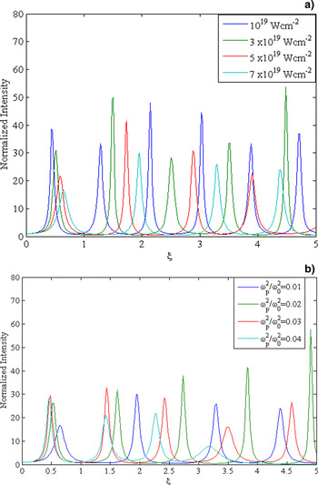
The IAW excited due to non-linear coupling between the ring-rippled laser beam and plasma in the presence of relativistic and ponderomotive non-linearities. This coupling arises on account of the change in the background density, that is, the motion of the charge carrier will be modified due to the relativistic–ponderomotive force in the plasma and will give rise to change in the non-linear current density. Thus, the amplitude of IAW, which depends upon the background density, gets strongly coupled to the laser beam. The magnitude of relativistic ponderomotive force is modified in the presence of the ring ripple because it depends on the intensity of the main beam and of the ring ripple. The presence of the ring ripple also leads to a change in modified ion density; consequently, the excitation of IAW is modified. To study the effect of ring-rippled laser beam in the presence of both relativistic and ponderomotive non-linearities on the excitation of IAW, we have numerically solved Eq. (20a) with the help of Eq. (21) to obtain the density profile of IAW at finite z. The intensity profile of the IAW depends on the beam width parameter (f a) of IAW, main beam (f 0), ring-rippled beam (f 1), and growth rate (g i) of ring ripple in the paraxial regime. The results are displayed in Figures 3a and 3b for the typical laser and plasma parameters as we have used in Figure 2. It is evident from the figures that the IAW gets excited due to non-linear coupling with intense laser beam. It is obvious from the figures that in the paraxial regime, the IAW becomes maximum at z = 0 and the intensity of the IAW decreases/increases with increase in laser intensity and plasma frequency respectively with normalized distance of propagation. This is due to the fact that the Landau damping term in Eq. (20a) and the growth rate are sensitive to the intensity of the IAW, which reduces the growth and intensity of the IAW.
(a) Variation in normalized intensity of IAW in the plasma with normalized distance (ξ = zc/ω0r 02) at maximum irradiance r 2 = r 12f 12(n + δ) for constant ωp2/ω02(=0.2) and for different laser beam intensities. (b) Variation in normalized intensity of IAW in the plasma with normalized distance (ξ = zc/ω0r 02) at maximum irradiance r 2 = r 12f 12(n + δ) for constant laser intensity (a = 3 × 10¹⁹ W/cm2) and for different plasma frequencies, when both relativistic and ponderomotive non-linearities are operative.

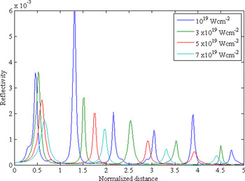
Equations (33) and (36), express the beam width parameter of the scattered wave and the back reflectivity of SBS, respectively, against the distance of propagation. The numerical results of Eq. (36) are presented in the form of Figure 4, which shows the variation of the SBS back reflectivity with normalized distance for different values of laser intensities around the maximum intensity of the ring ripple at r 2 = r 12f 12(n+δ). It has been observed that f 0, f 1, and f a jointly determine the focusing/defocusing of the scattered wave, and the SRS back reflectivity is strongly dependent upon the beam width parameter of the scattered wave, and intensity of the IAW. It is found that the back reflectivity of SBS is enhanced when both non-linearities are present and due to the contribution of ring ripple superimposed on the main beam in comparison with smooth Gaussian laser beam (Sodha et al., Reference Sodha, Umesh and Sharma1979; Mahmoud et al., Reference Mahmoud, Sharma, Kumar and Yadav1999; Sharma et al., Reference Sharma, Sharma, Rajput and Bhardwaj2009; Singh & Walia, Reference Singh and Walia2012; Sharma & Singh, Reference Sharma and Singh2013) where ponderomotive and relativistic non-linearities are separately taken into the account. Moreover, it is clearly evident from Figure 4 that the SBS reflectivity gets reduced with increase in laser intensity because the focusing of ring-rippled and main beams decreases with increasing the intensity of laser beam due to the combined effects of relativistic and ponderomotive non-linearities. The fluctuations in the reflectivity are on the account of minima in the dimensionless beam width parameters of main laser beam, ring-rippled beam, and IAW.
Variation in backscattered reflectivity (R) of SBS with normalized distance (ξ = zc/ω0r 02) for different values of laser intensities, when both relativistic and ponderomotive non-linearities are operative.

7. CONCLUSIONS
In conclusion, we develop a theoretical model for excitation of IAW and resulting SBBS in the collisionless plasma when relativistic–ponderomotive non-linearity is operative and ring-like spikes are superimposed on a high irradiance Gaussian laser beam. We have used the Wentzel–Kramers–Brillouin (WKB) and paraxial approximation in order to obtain analytical results concerning the physical conditions to achieve the self-focusing and intensity profiles of the main laser beam, ring ripple, IAW, and back reflectivity of SBS. The growth of ring ripple in the plasma significantly affected the intensity of IAW and the SBBS process. The intensity of IAW reduced at the higher value of laser intensity. The analytical expression for the ring ripple intensity [Eq. (9)] shows that the presence of ring ripple on the main laser beam enhanced the back reflectivity of the SBS process. The back reflectivity of SBS suppressed at higher intensity of the laser beam. The results of the present investigation may be useful for understanding the physics of the SBS process at high laser power flux in laser–plasma interaction where ring-like spikes are also present on the laser beam.
ACKNOWLEDGMENTS
We thank R.K. Singh, Centre for Energy Studies, Indian Institute of Technology Delhi (IITD), India for the important contributions to the numerical calculations. The authors are grateful to the Uttarakhand Council for Science & Technology (UCOST), Government of Uttarakhand, India for financial support.