


1. Introduction
The dynamics governing turbulent flows is associated with a large number of degrees of freedom required to describe the flow in a given domain. In the framework of Kolmogorov's famous  $K41$ theory for isotropic homogeneous turbulence (IHT) (Kolmogorov Reference Kolmogorov1941), we can obtain an estimate for the required number of the degrees of freedom from the ratio of the sizes between the largest and smallest length scales of the flow. This ratio is equal to the large-scale turbulent Reynolds number,
 $R=v \ell /\nu$, raised to a power of
 $9/4$ (
 $v$ is the large-scale velocity,
 $\ell$ the large-scale length scale and
 $\nu$ is the kinematic viscosity). Even though the degrees of freedom grow rapidly as
 $R$ increases, the accuracy of this number relies upon assumptions in
 $K41$ that are generally not satisfied in inhomogeneous settings, such as e.g. wall-bounded flows.
A dynamical-systems approach, on the other hand, associates the degrees of freedom with the dimension of the attractor underlying the turbulent state. Foias & Prodi (Reference Foias and Prodi1967) and Ladyzhenskaya (Reference Ladyzhenskaya1975) have shown that the dynamics of the Navier–Stokes equations asymptotically lie on finite-dimensional global attractors. The estimates of the dimension of the attractor, assuming the smoothness and global existence of the solutions of three-dimensional Navier–Stokes equations, obtained by this approach are in agreement with the estimate obtained from the K41 phenomenology (Doering & Gibbon Reference Doering and Gibbon1995; Foias et al. Reference Foias, Manley, Rosa and Temam2001; Robinson Reference Robinson2001).
The idea that not all degrees of freedom are equally important is certainly not a new concept. It is believed that turbulent flows are primarily driven by the large-scale coherent motions that are actively participating in the energy extraction from external energy inputs, whereas the small scales are responsible for dissipation of energy that is transferred to them from the larger scales through a series of nonlinear interactions. Additionally, the effect of the large-scale motions was shown to be imprinted on the small-scale statistics, as for example in turbulent wakes (Thiesset, Danaila & Antonia Reference Thiesset, Danaila and Antonia2014; Alves Portela, Papadakis & Vassilicos Reference Alves Portela, Papadakis and Vassilicos2020) and the formation of intense vorticity structures (‘worms’) within the dissipative scale of isotropic turbulence (Vela-Martín Reference Vela-Martín2021), raising questions about the universality of the Kolmogorov cascade.
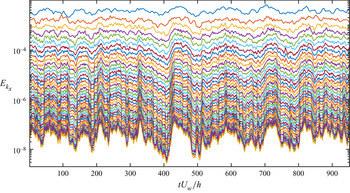
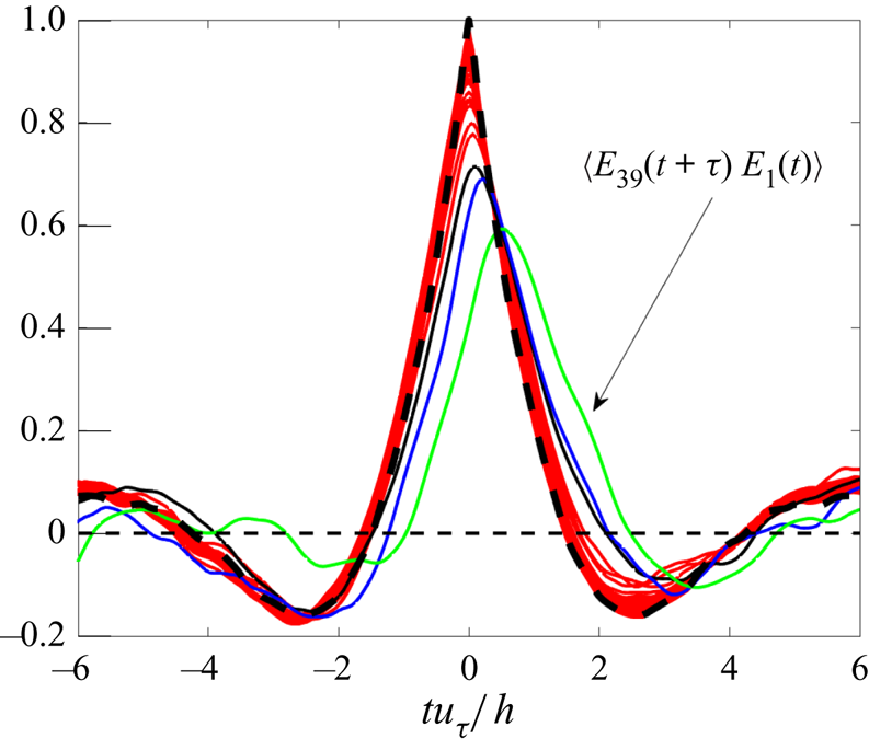
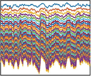
A striking example of influence of the large scales on the smaller scales investigated in this paper is exhibited in the time series of the energy density of the streamwise Fourier components of wall-bounded turbulence in streamwise periodic channels. Figure 1 shows an example from a simulation of plane Couette turbulence at  $R=1500$. It is evident that the higher-order streamwise components vary in unison. Figure 2 confirms that higher streamwise components vary in unison by plotting the normalized time-lag cross-correlation of the time series of the energy between the last streamwise component retained in the simulation with the other streamwise components. This synchronous behaviour suggests that the large scales (associated here with the gravest streamwise components) exert considerable influence on the structure and colour of the nonlinear interactions that transfer energy to the smaller scales. The above-mentioned results suggest also that the higher-order streamwise components may form a passive subspace of the dynamics that is synchronized by an active subspace spanned by the lower-order streamwise components of the turbulent flow.
Time series of the energy density of the 39 streamwise varying components in a simulation of Couette turbulence at  $R=1500$ (see table 1). Here
 $E_{k_x}$ indicates the energy density of the Fourier component with streamwise wavenumber
 $k_x= n \alpha$ where
 $\alpha =2{\rm \pi} / L_x$ is the smallest non-zero wavenumber allowed in the channel and
 $n=1,\ldots,39$;
 $E_{k_x}$ monotonically decreases with increasing wavenumber. Note how the higher harmonics (
 $n \geqslant 6$) vary in unison.

The normalized time-lag cross-correlation coefficient,  $\langle E_{39}(t+\tau ) E_{k_x}(t) \rangle$, of the energy,
 $E_{39}$, of the last streamwise Fourier component retained in the simulation of figure 1 (with streamwise wavenumber
 $39 \alpha$) with the energy of the
 $n$th streamwise component as a function of the time lag expressed in wall units (
 $u_\tau =0.0621 U_w$). The correlation with streamwise harmonics
 $n=1,2,3$ is indicated with a different colour. The lag autocorrelation
 $\langle E_{39}(t+\tau ) E_{39}(t) \rangle$ is indicated with the thick dash line. The energies of streamwise harmonics
 $E_{k_x}$ with
 $n \geqslant 4$ are strongly correlated with
 $E_{39}$.

Simulation parameters. The channel size in the streamwise, wall-normal and spanwise directions is  $[L_x,L_y,L_z]/h=[1.75{\rm \pi},2,1.2{\rm \pi} ]$, where
 $h$ is the half-width. Lengths in wall units are indicated by
 $[L_x^+,L_y^+,L_z^+]$. Here
 $N_x$,
 $N_z$ are the number of Fourier components after dealiasing and
 $N_y$ is the number of Chebyshev components. Here
 $R_{\tau } = h u_{\tau } / \nu$ is the Reynolds number of the simulation based on the friction velocity
 $u_{\tau }$ and
 $R = h U_w / \nu$ the bulk velocity Reynolds number according to the velocity at the wall
 $U_w$, the viscosity
 $\nu$ and the channel half-width
 $h$.
 $\Delta x^+$ and
 $\Delta z^+$ denote the time average streamwise and spanwise grid spacing in wall units.

Synchronization of chaotic systems (Pecora & Carroll Reference Pecora and Carroll1990) in general is commonly associated with collapsing subspaces that may exist in the dynamics, which have the property to attract all nearby trajectories onto a single solution lying on that subspace. The proof of the finiteness of the dimension of the attractor of the Navier–Stokes equations in periodic domains by Foias & Prodi (Reference Foias and Prodi1967) and Ladyzhenskaya (Reference Ladyzhenskaya1975) was based on the existence of such a globally synchronizable subspace. Specifically, Foias & Prodi (Reference Foias and Prodi1967) and Ladyzhenskaya (Reference Ladyzhenskaya1975) have shown that any solution of the Navier–Stokes equations can be recovered from its projection to a space of dimension  $n$ consisting of the
 $n$ gravest eigenmodes of the Stokes operator. The size of the subspace depends on the degree of dissipation and increases with the Reynolds number
 $R$ as predicted by the K41 phenomenology. The mechanism of synchronization described in the theory of Foias & Prodi (Reference Foias and Prodi1967) and Ladyzhenskaya (Reference Ladyzhenskaya1975) is essentially dissipative.
Turbulence synchronization of the small-scale motions by large-scale motions was investigated in two-dimensional and three-dimensional IHT by Yström & Kreiss (Reference Yström and Kreiss1998) and Henshaw, Kreiss & Yström (Reference Henshaw, Kreiss and Yström2003) who demonstrated that synchronization of the small scales can be achieved but the slaved subspace is larger than that predicted by the bounds of Foias & Prodi (Reference Foias and Prodi1967) and Ladyzhenskaya (Reference Ladyzhenskaya1975). More recent studies confirm and establish these results. Lalescu, Meneveau & Eyink (Reference Lalescu, Meneveau and Eyink2013) demonstrated that three-dimensional IHT flow fields with scales below approximately 20 Kolmogorov dissipation lengths can be slaved by the larger-scale motions. Similar estimates were obtained by Yoshida, Yamaguchi & Kaneda (Reference Yoshida, Yamaguchi and Kaneda2005) and Clark Di Leoni, Mazzino & Biferale (Reference Clark Di Leoni, Mazzino and Biferale2020) in their investigations of data assimilation of small scales from knowledge of the large scales in IHT. Henshaw et al. (Reference Henshaw, Kreiss and Yström2003) also conjectured that the disparity found in the size of the synchronizable subspaces should be attributed to the enhanced dissipation that occurs in the strong deformation regions forming in the flow, which is not captured in the analysis of Foias & Prodi (Reference Foias and Prodi1967) and Ladyzhenskaya (Reference Ladyzhenskaya1975).
Another mechanism of synchronization is revealed in the restricted nonlinear (RNL) or quasilinear (QL) approximations of the dynamics of wall-bounded turbulent flows in streamwise periodic channels. In this approximation, the flow is separated in its streamwise-mean component  ${\boldsymbol {u}}_0$ and streamwise-varying component
 $\tilde {{\boldsymbol {u}}}$, the streamwise mean evolves with the Navier–Stokes equations without any approximation while the dynamics of the streamwise-varying components is restricted to QL interaction with the streamwise mean and dissipation. In this approximation the nonlinear interactions among the streamwise-varying components are neglected in the dynamics of the streamwise-varying components but are included in the streamwise-mean equations. It has been shown that this approximation self-sustains a realistic state of turbulence in wall-bounded flows (Farrell & Ioannou Reference Farrell and Ioannou2012; Bretheim, Meneveau & Gayme Reference Bretheim, Meneveau and Gayme2015; Farrell et al. Reference Farrell, Ioannou, Jiménez, Constantinou, Lozano-Durán and Nikolaidis2016; Farrell, Gayme & Ioannou Reference Farrell, Gayme and Ioannou2017). The RNL turbulent state sustains a few streamwise Fourier components of the flow and has the property that all the streamwise-varying components, both those that are sustained at finite energy and those that decay to zero, can be synchronized by the time-varying streamwise-mean flow component
 ${\boldsymbol {u}}_0$ (Farrell & Ioannou Reference Farrell and Ioannou2017). The synchronization in this case occurs because of the interaction with the mean: the streamwise components that are sustained by the time-varying mean flow have been adjusted to neutral parametric stability, while the others parametrically decay. The components that are sustained by the parametric interaction with the mean are the neutral modes of the time-varying state (the neutral Lyapunov vectors) and we will be referring to them as ‘parametrically active’ or ‘RNL active’; the subspace that decays will be referred to as ‘parametrically passive’ or ‘RNL passive’. Of course in Navier–Stokes turbulence, energy transfers to the streamwise-varying components by nonlinear interactions among them are also present, and the question arises to what degree these can be dominated by transfers from the parametrically active scales thus rendering the parametrically passive subspace synchronizable. In this paper we investigate whether such synchronization occurs in parallel Couette turbulence in streamwise and spanwise periodic channels.
The paper is organized as follows. We first formulate the synchronization problem (§ 2) and determine the components of the flow that can be synchronized using linear theory (§ 3). We then show that the predictions of linear theory lead to global synchronization (§ 4.1) and we investigate the relation of the synchronization subspaces to the active and passive subspaces of the corresponding RNL turbulence (§ 4.2). Finally we discuss the energetics and determine that the scales that synchronize have streamwise length smaller than 130 wall units (§ 5).
2. Formulation
We consider incompressible parallel Couette flows in channels that are periodic in the streamwise  $x$ and spanwise
 $z$ directions, with the channel plane walls at
 $y=\pm h$. In order to examine whether the smaller streamwise scales can be slaved to the larger streamwise scales or, equivalently, whether the smaller streamwise scales can be synchronized by the larger ones, we split the flow field
 ${\boldsymbol {u}}$ into streamwise Fourier components containing the longer streamwise scales,
 \begin{equation} {\boldsymbol{u}}_<{=} \sum_{0\leqslant n \leqslant N-1} \hat{{\boldsymbol{u}}}_{n } (y,z,t) \textrm{e}^{\textrm{i} n \alpha x}, \end{equation}
where  $k_x= n \alpha$, with
 $\alpha = 2 {\rm \pi}/ L_x$, is the wavenumber of the
 $n$th streamwise harmonic in the periodic channel with streamwise length
 $L_x$, and the smaller scales,
 \begin{equation} {\boldsymbol{u}}_{>}= \sum_{n \geqslant N} \hat{{\boldsymbol{u}}}_{n } (y,z,t) \textrm{e}^{\textrm{i} n \alpha x}, \end{equation}
with  ${\boldsymbol {u}} = {\boldsymbol {u}}_< +{\boldsymbol {u}}_>$.
The equations governing these flow fields are obtained by projecting the incompressible Navier–Stokes equation on the corresponding Fourier subspaces (Frisch Reference Frisch1995). The large scales are governed by the Navier–Stokes,
 \begin{equation} \partial_t {\boldsymbol{u}}_<{=} -P_< \left ( ({\boldsymbol{u}}_<{+}{\boldsymbol{u}}_>) \boldsymbol{\cdot} \boldsymbol{\nabla} ({\boldsymbol{u}}_<{+}{\boldsymbol{u}}_>) - R^{{-}1} \Delta {\boldsymbol{u}}_< \right ), \end{equation}
where  $P_<$ is the Leray projection on the space spanned by streamwise harmonics
 $0,\ldots,N-1$, coupled to the Navier–Stokes for the smaller scales,
 \begin{equation} \partial_t {\boldsymbol{u}}_>{=} -P_> \left ( ({\boldsymbol{u}}_<{+}{\boldsymbol{u}}_>) \boldsymbol{\cdot} \boldsymbol{\nabla} ({\boldsymbol{u}}_<{+}{\boldsymbol{u}}_>) - R^{{-}1} \Delta {\boldsymbol{u}}_> \right), \end{equation}
with  $P_>$ the Leray projection on the space spanned by the
 $n \geqslant N$ streamwise harmonics. The above equations are non-dimensional with lengths non-dimensionalized by the half-channel width
 $h$, velocities by the streamwise velocity
 $U_w$ at the walls and time by
 $h/U_w$. The Reynolds number is defined as
 $R=U_w h/ \nu$, with
 $\nu$ the kinematic viscosity. The flow velocity satisfies the no-slip boundary condition
 ${\boldsymbol {u}} = \pm \hat {{\boldsymbol {x}}}$ at the channel walls
 $y=\pm 1$ (
 $\hat {{\boldsymbol {x}}}$ is the unit vector in the streamwise direction).
Synchronization of the smaller scales to the larger scales is achieved when an arbitrary smaller-scale flow field,  $\boldsymbol{v}_>$, governed by the Navier–Stokes equations
 \begin{equation} \partial_t \boldsymbol{v}_>{=} -P_> \left ( ({\boldsymbol{u}}_<{+}\boldsymbol{v}_>) \boldsymbol{\cdot} \boldsymbol{\nabla} ({\boldsymbol{u}}_<{+}\boldsymbol{v}_>) - R^{{-}1} \Delta \boldsymbol{v}_> \right ), \end{equation}
in the smaller Fourier scale subspace with prescribed large-scale field  ${\boldsymbol {u}}_<$ satisfying (2.3) and (2.4), converges to
 ${\boldsymbol {u}}_>$, i.e. synchronization with the direct numerical simulation (DNS) realization is achieved when
 $\lim _{t\to \infty } || \boldsymbol{v}_>(t)- {\boldsymbol {u}}_> (t)|| = 0$. We choose as metric
 $|| \cdot ||$, the square root of the kinetic energy density of the flow.
Synchronization in the linear limit is guaranteed when the top Lyapunov exponent of smaller-scale perturbations to (2.4) linearized about a solution  ${\boldsymbol {u}}_<$ and
 ${\boldsymbol {u}}_>$ of the NS (2.3) and (2.4) is negative. In that case, any flow
 $\boldsymbol{v}_>$ adequately close to
 ${\boldsymbol {u}}_>$ is guaranteed to synchronize. However, this criterion does not guarantee synchronization of states
 $\boldsymbol{v}_>$ that are not in the neighbourhood of
 ${\boldsymbol {u}}_>$.
The leading Lyapunov exponent is obtained by calculating the asymptotic exponential growth rate of the amplitude of the difference field  ${\boldsymbol {u}^\prime_>}=\boldsymbol{v}_>-{\boldsymbol {u}}_>$, governed by the linearized equation (2.5) about the DNS solution
 ${\boldsymbol {u}}_<+{\boldsymbol {u}}_>$:
 \begin{equation} \partial_t {\boldsymbol {u}^\prime_>} ={-}P_> \left ( ({\boldsymbol{u}}_<{+}{\boldsymbol{u}}_>) \boldsymbol{\cdot} \boldsymbol{\nabla} {\boldsymbol {u}^\prime_>} + {\boldsymbol {u}^\prime_>} \boldsymbol{\cdot} \boldsymbol{\nabla} ({\boldsymbol{u}}_<{+}{\boldsymbol{u}}_>) - R^{{-}1} \Delta {\boldsymbol {u}^\prime_>} \right ). \end{equation}
The linearized equations (2.6), which are referred to as the variational equations, determine the asymptotic stability of the time-dependent flow  ${\boldsymbol {u}}_<+{\boldsymbol {u}}_>$ of the DNS to perturbations
 ${\boldsymbol {u}^\prime_>}$ with streamwise wavenumbers
 $k_x \geqslant N \alpha$. The top Lyapunov exponent of (2.6),
 $\lambda _N$, for truncation at
 $N$ is defined as
 \begin{equation} \lambda_N = \overline{\lim_{t^{\prime} \to \infty}}\frac{1}{t^{\prime}} \log \left (\frac{||{\boldsymbol {u}^\prime_>}(t+t^{\prime})||}{||{\boldsymbol {u}^\prime_>}(t)||} \right ). \end{equation}
Previous studies presented results on the Lyapunov exponent(s) for  $N=0$, in our notation for the
 $\lambda _0$, cf. Keefe, Moin & Kim (Reference Keefe, Moin and Kim1992) and Nikitin (Reference Nikitin2008, Reference Nikitin2018). The
 $N=0$ Lyapunov exponent determines the sensitivity of the whole turbulent flow trajectory
 ${\boldsymbol {u}}$ to perturbations that have power in all the streamwise Fourier components.
A negative Lyapunov exponent,  $\lambda _N<0$, implies exponential decay of the perturbation field
 ${\boldsymbol {u}^\prime_>}$ in the linear approximation. However, in the channel flows considered, we find that all
 ${\boldsymbol {u}}^{\prime}$, of any amplitude, decay to zero, at the rate of the Lyapunov exponent
 $\lambda _N$ of the decomposition, indicating that the
 ${\boldsymbol {u}}_>$ flow is globally attracting. This should be probably anticipated from the related theorems of Foias & Prodi (Reference Foias and Prodi1967) and Ladyzhenskaya (Reference Ladyzhenskaya1975) that show, based on projections on the eigenfunctions of the Stokes operator, that the attractor of the Navier–Stokes equations (assuming regularity of the solutions in the case of three dimensions) is finite dimensional and that the small scales of the flow are eventually necessarily globally synchronizable (cf. also the recent studies of Foias et al. (Reference Foias, Manley, Rosa and Temam2001), Robinson (Reference Robinson2001) and Lalescu et al. (Reference Lalescu, Meneveau and Eyink2013)). Exponential approach to synchronization and variation of this exponential rate with the scale of the slaved subspace has been also found in IHT by Yström & Kreiss (Reference Yström and Kreiss1998), Hayashi, Ishihara & Kaneda (Reference Hayashi, Ishihara and Kaneda2003), Yoshida et al. (Reference Yoshida, Yamaguchi and Kaneda2005) and Lalescu et al. (Reference Lalescu, Meneveau and Eyink2013). We show here that synchronization can be achieved very efficiently if the projection is based on the streamwise Fourier components of the flow.
3. Lyapunov exponents of the turbulent flow to streamwise-restricted perturbations
We consider DNS solutions of turbulent Couette flow at the three Reynolds numbers: (i)  $R=600$ that sustains turbulence with
 $R_\tau = 45$; (ii)
 $R=1500$ with
 $R_\tau = 93$; and (iii)
 $R=2250$ with
 $R_{\tau }=134$ and calculate the top Lyapunov exponents
 $\lambda _N$ of (2.6) for various truncations
 $N$. The simulations are performed with an in-house developed DNS code with graphics processing unit acceleration written in MATLAB that solves the Navier–Stokes equations in wall-normal velocity/vorticity formulation (Kim, Moin & Moser Reference Kim, Moin and Moser1987). The code employs Chebyshev discretization on the wall-normal direction and a finite difference grid on the streamwise and spanwise directions which are treated pseudospectrally and are dealiased following the
 $2/3$ rule. Time stepping is accomplished with a Crank–Nicolson and a third-order Runge–Kutta scheme for the viscous and advective terms, respectively. Parameters of the simulations are summarized in table 1. The mean velocity profile,
 $U(y) = \int _0^T \int _0^{L_z} \hat {{\boldsymbol {x}}} \boldsymbol {\cdot } {{\boldsymbol {u}}}_0 \,\textrm {d}z \,\textrm {d}t / (T L_z)$ where
 ${\boldsymbol {u}}_0= \int _0^{L_x} {{\boldsymbol {u}}}\,{\textrm {d} x} /L_x$ is the streamwise-mean velocity; the r.m.s. profile of the fluctuations averaged over the streamwise and spanwise directions,
 $(u_{rms}^{\prime2},v_{rms}^{\prime2},w_{rms}^{\prime2})= \int _0^T \int _0^{L_z} \int _0^{L_x} (u^{\prime2},v^{\prime2},w^{\prime2})\,{\textrm {d} x} \,\textrm {d}z \,\textrm {d}t/(T L_z L_x )$, with
 $(u^{\prime},v^{\prime},w^{\prime})={\boldsymbol {u}}-U(y) \hat {{\boldsymbol {x}}}$; and the mean tangential Reynolds stress profile
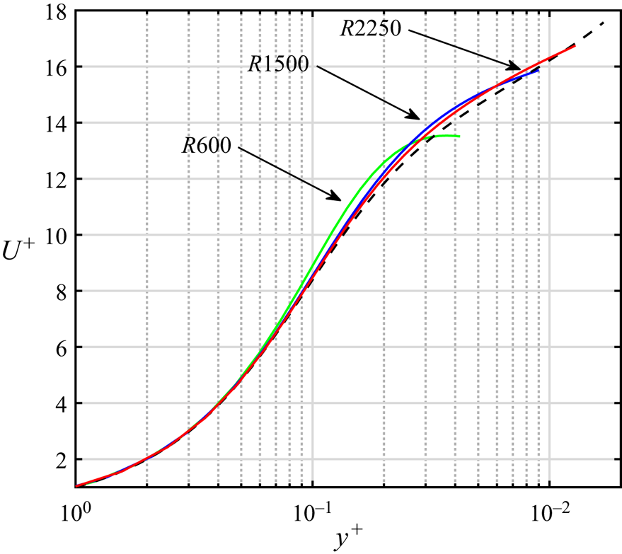
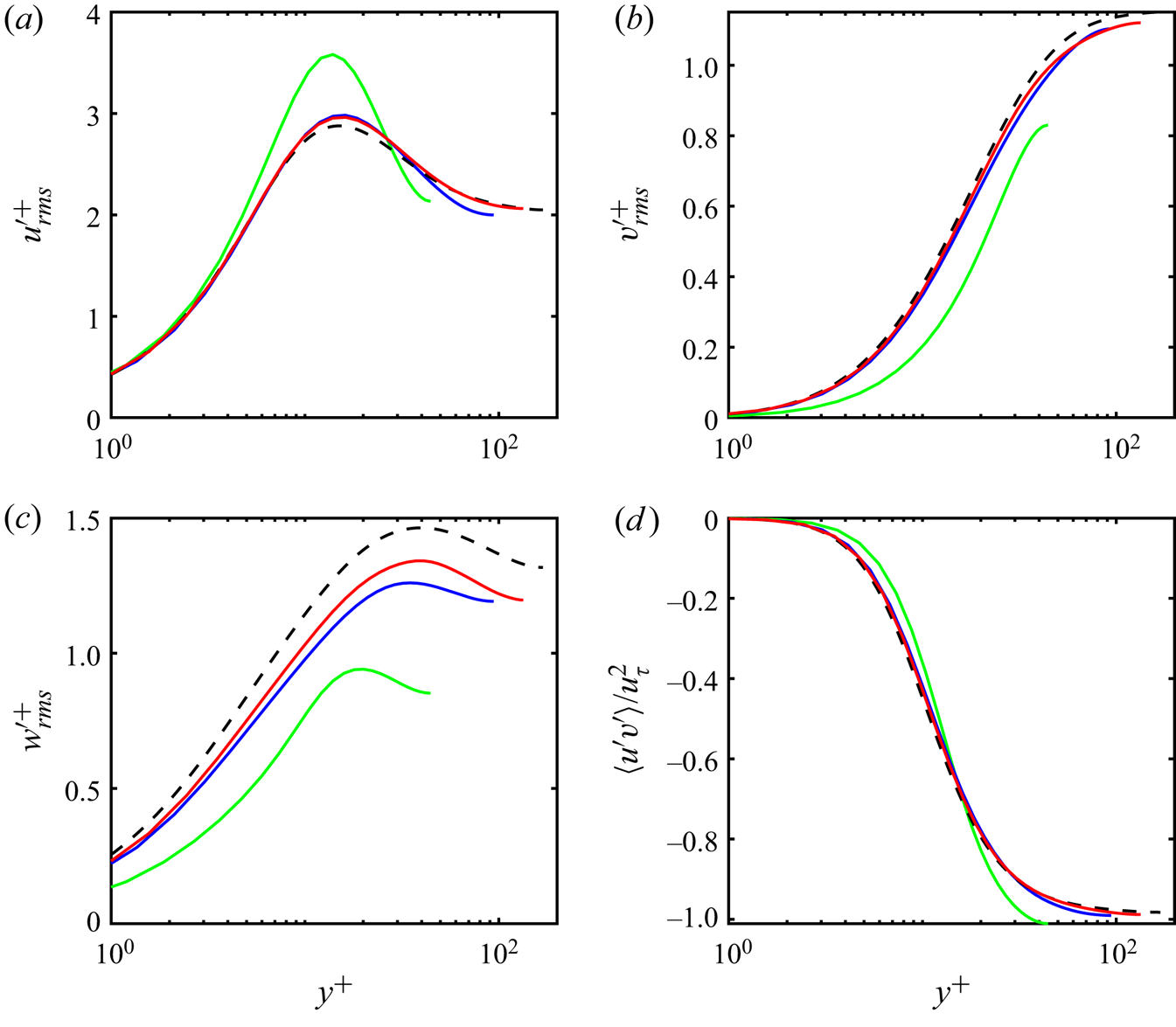
 $\langle u^{\prime} v^{\prime} \rangle = \int _0^T \int _0^{L_z} \int _0^{L_x} u^{\prime} v^{\prime} \,{\textrm {d} x} \,\textrm {d}z \,\textrm {d}t/(T L_z L_x )$ averaged over the streamwise and spanwise directions and their comparison with the literature are plotted in figures 3 and 4.
Streamwise, spanwise and time average of the streamwise velocity component  $U(y)$ in viscous wall units for simulations in table 1. The dashed line indicates the mean velocity profile obtained by Pirozzoli, Bernardini & Orlandi (Reference Pirozzoli, Bernardini and Orlandi2014) for a larger channel at
 $R_{\tau }=171$.

One-point statistics for the simulations R600 (green), R1500 (blue) and R2250 (red) in table 1. (a–c) Root mean square (r.m.s.) profiles for the velocity fluctuation components  $(u^{\prime},v^{\prime},w^{\prime})={\boldsymbol {u}}-U(y) \hat {{\boldsymbol {x}}}$ in viscous units. Here
 $U$ is the streamwise, spanwise and time average of the streamwise velocity component. (d) Streamwise, spanwise and time average profile of tangential Reynolds stress
 $\langle u^{\prime} v^{\prime} \rangle$ in viscous units. The dashed line in each graph indicates the same statistics obtained by Pirozzoli et al. (Reference Pirozzoli, Bernardini and Orlandi2014) at
 $R_{\tau }=171$.

The numerical integration of (2.6) for the determination of the top Lyapunov exponent is initialized from a randomly generated, divergence-free initial condition that lies on the specified subspace, which is kept infinitesimal by normalization at the end of each time step. The fields  ${\boldsymbol {u}}_<$ and
 ${\boldsymbol {u}}_>$ appearing in (2.6) are determined simultaneously by the DNS of (2.3) and (2.4). An instantaneous growth rate,
 $\lambda (t)$, is then calculated from the ratio of
 $||{\boldsymbol {u}^\prime_>}||$ at time
 $t$ and at the adjacent time step
 $t+\Delta t$ before normalization,
 \begin{equation} \lambda(t)= \frac{1}{\Delta t} \log \left (\frac{||{\boldsymbol {u}^\prime_>}(t+\Delta t)||}{ ||{\boldsymbol {u}^\prime_>}(t)||} \right ). \end{equation}
The  $\lambda (t)$ are highly variable in time, but in the long-term their average value converges to the Lyapunov exponent
 $\lambda _N$, for each choice of
 $N$. The flow states associated with the Lyapunov exponents have non-negligible spectral coefficients in all included streamwise wavenumbers (i.e.
 $k_x \geqslant N \alpha$).
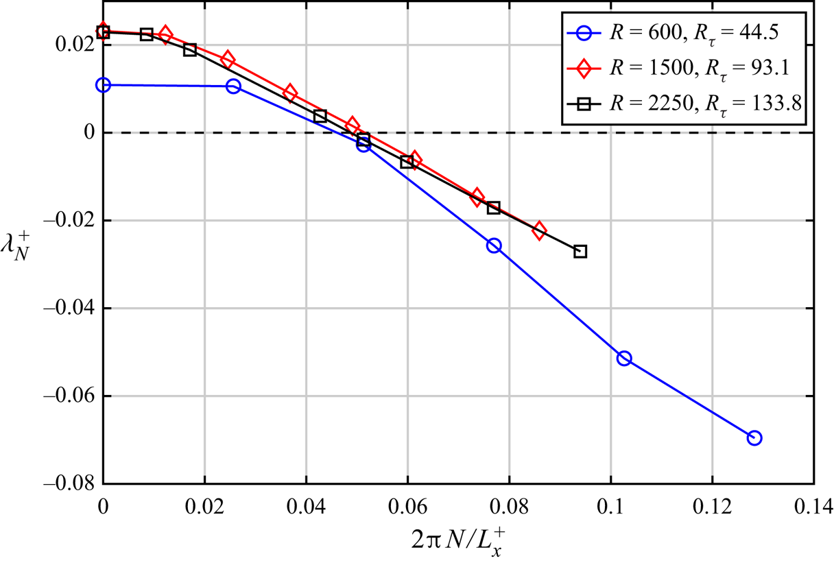
The resulting top Lyapunov exponents are plotted in figure 5 as a function of the order of truncation  $N$. The top Lyapunov exponents for
 $N=0$, associated with the sensitivity of the full turbulent trajectory, collapse to the value
 $\lambda ^+_0 \approx 0.023$ for
 $R=1500$ and
 $R=2250$ when scaled in wall units. This agrees with the constant Lyapunov exponent
 $\lambda ^+_0 = 0.021$ obtained by Nikitin (Reference Nikitin2008) in plane channel and pipe flows with
 $R_{\tau }$ in the range from
 $140$ to
 $320$. The smaller value
 $\lambda ^+_0=0.01$ obtained at
 $R=600$ is expected as the sensitivity of the flow is diminished as the size of the channel approaches the minimal channel dimensions (Inubushi, Takehiro & Yamada Reference Inubushi, Takehiro and Yamada2015; Nikitin Reference Nikitin2018). As
 $N$ increases the top Lyapunov exponent monotonically decreases and eventually becomes negative at
 $N_c$, indicating that subspaces with
 $N\geqslant N_c$ are synchronizable in the linear limit. The critical truncation
 $N_c$ is different for each Reynolds number. However, when we scale the wavelengths and growth rates with the corresponding friction velocities, the predicted threshold streamwise wavelength at which
 $\lambda _N$ becomes negative collapses to the value
 $\ell _x^+=130$. We observe that the
 $\lambda _N^+$ for
 $R=1500$ and
 $R=2250$ collapse to an asymptotic curve with increasing Reynolds number, showing that the wall-unit scaling remains valid across the top
 $N$ subspaces, indicating that the buffer-layer dynamics associated with the self-sustaining process is in control at these Reynolds numbers.
The top Lyapunov exponents,  $\lambda ^+_N$, of the perturbation equations (2.6) as a function of the wavenumber
 $2 {\rm \pi}N / L_x^+$ of the streamwise component
 $N$. Here
 $N$ is the gravest Fourier component of the perturbation
 ${\boldsymbol {u}^\prime_>}$. The Lyapunov exponent is expressed in wall units
 $u^2_{\tau }/\nu$. For
 $R=600$ we plot
 $\lambda ^+_N$ for
 $N=0,\ldots,5$ (blue circles), for
 $R=1500$ we plot
 $N=0,\ldots,7$ (red diamonds) and
 $N=0,1,2,5,6,7,9,11$ for
 $R=2250$ (black squares). This figure indicates that at
 $R=600$ the critical streamwise harmonic is
 $N_c=2$, i.e. the
 ${\boldsymbol {u}}_<$ with streamwise harmonics
 $n=0,1$ synchronizes
 ${\boldsymbol {u}}_>$ in the linear limit. It is verified in § 4.1 that nonlinear simulations synchronize at the rate predicted by the Lyapunov exponents of this figure. At
 $R=1500$ synchronization in the linear limit occurs for
 $N_c=5$ when the
 ${\boldsymbol {u}}_<$ field includes streamwise harmonics
 $n=0,1,2,3,4$. At
 $R=2250$,
 $N_c=6$ and the
 ${\boldsymbol {u}}_<$ field comprised of
 $n=0,1,2,3,4,5$ synchronizes the
 ${\boldsymbol {u}}_>$ flow.

4. Synchronization experiments
4.1. Determination of the active subspace in Couette turbulence
To perform the synchronization experiment, we couple two DNSs, one solving for the total velocity and a second one where the components of the  ${\boldsymbol {u}}_<$ subspace obtained from the first simulation are imposed to the second, while solving (2.5) for the
 $\boldsymbol{v}_>$ flow field which is now initialized from an arbitrary state and not necessarily close to
 ${\boldsymbol {u}}_>$. According to linear theory, any
 $\boldsymbol{v}_>$ field close to
 ${\boldsymbol {u}}_>$ will synchronize to
 ${\boldsymbol {u}}_>$ for truncations
 $N\geqslant N_c$ for which
 $\lambda _N<0$. However, we find that all
 $\boldsymbol{v}_>$ in all cases of table 1 will synchronize to
 ${\boldsymbol {u}}_>$ if
 $N\geqslant N_c$, irrespective of the initial magnitude of the deviation of the
 $\boldsymbol{v}_>$ from
 ${\boldsymbol {u}}_>$. We also verify that even
 $\boldsymbol{v}_>$ states that are initially zero synchronize at the rate predicted by
 $\lambda _N$. This property of exponential decay of the
 $\boldsymbol{v}_>$ field to
 ${\boldsymbol {u}}_>$ is referred to as the strong squeezing property which may indicate that the attractor basin of
 ${\boldsymbol {u}}_<$ covers the whole space and the subspace
 ${\boldsymbol {u}}_>$ is uniquely determined by the subspace
 ${\boldsymbol {u}}_<$, since it attracts any initial condition
 $\boldsymbol{v}_>$, forming an inertial manifold (Foias et al. Reference Foias, Manley, Rosa and Temam2001; Robinson Reference Robinson2001).
The critical truncation is predicted from the calculation of the Lyapunov exponents to be  $N_c=2$ for
 $R600$,
 $N_c=5$ for
 $R1500$ and
 $N_c=6$ for
 $R2250$. Examples of synchronization are shown in figure 6 for
 $R600$ and in figure 7(a) for
 $R2250$. The exponential convergence of
 $\boldsymbol{v}_>$ to
 ${\boldsymbol {u}}_>$ at the rate of the predicted
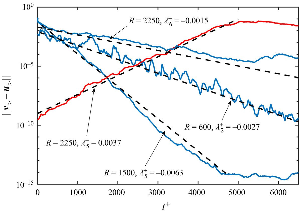
 $\lambda _N$ is verified in figure 8, which shows asymptotic exponential decay of the difference
 $|| \boldsymbol{v}_> - {\boldsymbol {u}}_>||$ to numerical precision. This asymptotic decay was confirmed in all the experiments we performed with large initial perturbations to the
 ${\boldsymbol {u}}_>$ state. Note that all streamwise components of
 $\boldsymbol{v}_>$ converge to
 ${\boldsymbol {u}}_>$ at the same rate, indicating that the Lyapunov vector corresponding to
 $\lambda _N$ has power at all retained streamwise wavenumbers. A case where synchronization is not possible is shown in figure 7(b) for
 $R2250$ and
 $N=5$. An initially infinitesimal difference
 $|| \boldsymbol{v}_> - {\boldsymbol {u}}_>||$ grows exponentially (the red line shown in figure 8) at the rate of
 $\lambda _5$ and the
 $\boldsymbol{v}_>$ subspace diverges from the
 ${\boldsymbol {u}}_>$ subspace.
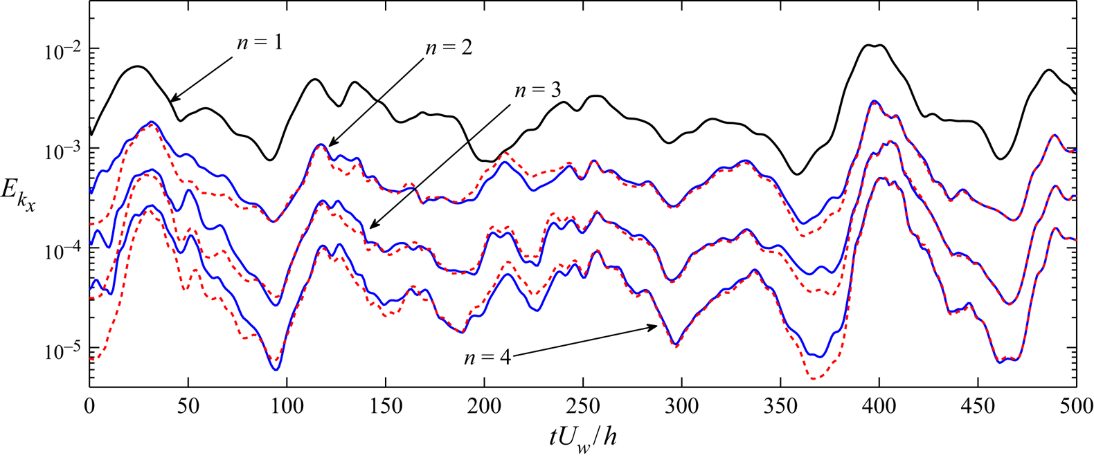
Time series of the energy density  $E_{k_x}$ of the first four streamwise-varying components in the
 $R=600$ simulation (solid lines). The critical truncation that achieves synchronization in this channel is
 $N_c=2$. In this experiment the
 ${\boldsymbol {u}}_<$ truncated with
 $N=2$ (shown with solid black line is the
 $n=1$ component) succeeds in synchronizing
 $\boldsymbol{v}_>$ (dotted red lines) to the
 ${\boldsymbol {u}}_>$ (solid blue lines) of the DNS (shown are components
 $n=2,3,4$). The exponential rate of convergence towards synchronization is λ = −0.01 U w/h (
 $\lambda^+=-0.0027$) consistent with the decay estimated from the Lyapunov exponent
 $\lambda _2$ of figure 5.

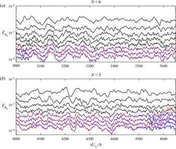
Time series of the energy density  $E_{k_x}$ of the first eight streamwise-varying components of the DNS of plane Couette turbulence at
 $R=2250$ (
 $R_\tau = 134$). The critical truncation that achieves synchronization in this channel is
 $N_c=6$. (a) Here
 ${\boldsymbol {u}}_<$ truncated with
 $N=6$ (shown with solid black lines are the
 $n=1,2,3,4,5$ components) succeeds in synchronizing
 $\boldsymbol{v}_>$ (dotted red lines) to the
 ${\boldsymbol {u}}_>$ (solid blue lines) of the DNS (shown are components
 $n=6,7,8$). The exponential rate of synchronization is
 $\lambda = -0.012 U_w/h$ (
 $\lambda^+ = - 0.0015$) in agreement with the Lyapunov exponent
 $\lambda _6$ of figure 5; (b)
 ${\boldsymbol {u}}_<$ truncated with
 $N=5$ (shown with solid black lines are the
 $n=1,2,3,4$ components) fails to synchronize
 $\boldsymbol{v}_>$ (dotted red lines) to the
 ${\boldsymbol {u}}_>$ (solid blue lines) of the DNS (shown are the
 $n=5,6,7,8$ components) and diverges at the rate of the Lyapunov exponent
 $\lambda _5=0.030 U_w/h$ (
 $\lambda_5^+ = 0.0037$, cf. figure 5). These experiments show that truncations with
 $N< N_c$ do not lead to synchronization while those with
 $N\geqslant N_c$ do.

The approach (blue lines) towards and the deviation (red line) from synchronization of the  $\boldsymbol{v}_>$ subspace, measured by the state error norm,
 $|| \boldsymbol{v}_> - {\boldsymbol {u}}_>||$, as a function of time expressed in wall units is shown to be asymptotically exponential at the rate of the Lyapunov exponent
 $\lambda _N^+$ (dashed), cf. figure 5. Shown are the synchronization of the
 $N=2$ subspace at
 $R=600$ (cf. figure 6), of the
 $N=5$ subspace at
 $R=1500$ and of the
 $N=6$ subspace at
 $R=2250$ (cf. figure 7a). In the last example the initial perturbation had
 $|| \boldsymbol{v}_>(0) - {\boldsymbol {u}}_>(0)||/||{\boldsymbol {u}}_>(0)||=1.6$. This example demonstrates that even large perturbations to the
 ${\boldsymbol {u}}_>$ state synchronize if the truncation is performed at the component
 $N_c$ predicted from linear theory. Conversely, small perturbations to the
 ${\boldsymbol {u}}_>$ state deviate at truncations with
 $N< N_c$ at the predicted rate of the Lyapunov exponent, as shown for the
 $N=5$ subspace at
 $R=2250$ (cf. figure 7b).

The minimal  ${\boldsymbol {u}}_<$ field that leads to synchronization is referred to as the active or determining subspace and the
 ${\boldsymbol {u}}_>$ as the passive or slave subspace. For the chosen channel the active subspace was determined to have
 $N_c=2$ components at
 $R=600$,
 $N_c=5$ at
 $R=1500$ and
 $N_c=6$ at
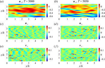
 $R=2250$. It is informative to see the structure of the active and passive components of the flow in an experiment of synchronization. Indicative active
 ${\boldsymbol {u}}_<$ and passive
 ${\boldsymbol {u}}_>$ velocity fields and the passive field
 $\boldsymbol{v}_>$ before and after synchronization for
 $R2250$ with
 $N=6$ are shown in figures 9 and 10 at the initial time
 $U_w T/h=5000$ when an arbitrary
 $\boldsymbol{v}_>$ is imposed and at
 $U_w T/h=5050$ when
 $\boldsymbol{v}_>$ has been synchronized to
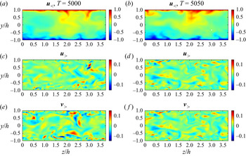
 ${\boldsymbol {u}}_>$. The cross-flow and spanwise (
 $y - z$) plane cross-section (figure 9) shows that the amplitude of the active
 ${\boldsymbol {u}}_>$ component is substantial, it reaches a velocity of
 $0.15U_w$ and is more prominent in the region surrounding the buffer-layer streaks. These plots also show the streaky large-scale inhomogeneous structure of the
 ${\boldsymbol {u}}_<$ active subspace. Note that the passive
 ${\boldsymbol {u}}_>$ subspace has substantial velocity amplitudes. The small-scale field
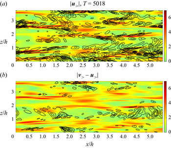
 ${\boldsymbol {u}}_>$ is located in the regions of large scale strain, shown in figure 11(a), and the error field at the intermediate time
 $U_w T/h=5018$ is predominantly in the regions of low strain as shown in figure 11(b) (cf. also supplementary movie 1 available at https://doi.org/10.1017/jfm.2021.1054). This is expected because deformation regions induce enhanced perturbation growth and also accelerate viscous decay (cf. Craik & Criminale Reference Craik and Criminale1986; Farrell & Ioannou Reference Farrell and Ioannou1993). The concentration of the
 ${\boldsymbol {u}}_>$ field in regions of high strain supports the conjecture of Henshaw et al. (Reference Henshaw, Kreiss and Yström2003) who proposed that the reason the initial estimates of the size of the synchronizable subspace were too conservative was because they did not account for the enhanced dissipation that occurs in the deformation regions. Also when
 $N \leqslant 5$ and synchronization fails the instabilities are seen to arise in the strain regions (cf. supplementary movie 2). This is consistent with the findings of Nikitin (Reference Nikitin2018) who noted that the
 $N=0$ Lyapunov vectors are located in the shear regions of the streak.
Contours in a  $y - z$ plane cross-section of two snapshots of the streamwise velocity component of the
 ${\boldsymbol {u}}_<$,
 ${\boldsymbol {u}}_>$ and
 $\boldsymbol{v}_>$ flow fields in DNS at
 $R=2250$ and
 $N=6$. The
 ${\boldsymbol {u}}_<$ includes streamwise harmonics
 $n=0,\ldots,5$. Panels (a,c,e) show the initial state of the synchronization experiment at
 $U_w T /h =5000$. Initially
 $|| \boldsymbol{v}_> - {\boldsymbol {u}}_>||=0.067$ while at
 $U_w T /h =5050$ the state has been almost synchronized with
 $|| \boldsymbol{v}_> - {\boldsymbol {u}}_>||=0.012$.

Contours in a  $x - z$ plane cross-section at
 $y/h=-0.77$ of the snapshots in figure 9 of the streamwise velocity component of the
 ${\boldsymbol {u}}_<$,
 ${\boldsymbol {u}}_>$ and
 $\boldsymbol{v}_>$ flow fields in DNS at
 $R=2250$. The
 ${\boldsymbol {u}}_<$ includes streamwise harmonics
 $n=0,\ldots, 5$.

Contours (in colour) of the maximum eigenvalue of the rate of strain tensor  $( \partial _i u_{j,<} + \partial _j u_{i,<})/2$ of the large-scale
 ${\boldsymbol {u}}_<$ flow on a
 $z - x$ plane at
 $y/h=-0.77$, at the intermediate time
 $U_w T/h=5018$ of the synchronization experiment shown in figure 7(a). Solid black lines indicate contours of the amplitude of: (a) the small-scale
 ${\boldsymbol {u}}_>$ flow and (b) of the error
 $\boldsymbol{v}_>-{\boldsymbol {u}}_>$, at levels between 0.22 and 1.1 of the maximum of
 $|{\boldsymbol {u}}_>|$ at this plane. This figure shows that the
 ${\boldsymbol {u}}_>$ field is concentrated in regions of high strain, whereas the error field
 $\boldsymbol{v}_>-{\boldsymbol {u}}_>$ in these regions decays rapidly and is predominantly located in regions of smaller large-scale strain.

4.2. Synchronization of single streamwise harmonics and their relation to the components sustained in RNL
In the RNL or QL approximation of the dynamics of wall-bounded flows, the streamwise-mean flow  ${\boldsymbol {u}}_0(y,z,t)=\int _0^{L_x} {\boldsymbol {u}} \,{\textrm {d} x} /L_x$ evolves under the full Navier–Stokes dynamics without any approximation, while the dynamics of the streamwise-varying flow,
 $\tilde {{\boldsymbol {u}}}(x,y,z,t)={\boldsymbol {u}}-{\boldsymbol {u}}_0$, is restricted to QL interaction with
 ${\boldsymbol {u}}_0$, neglecting altogether the nonlinear interactions between the
 $\tilde {{\boldsymbol {u}}}$. The equations governing the RNL dynamics are
 $$\begin{gather} \partial_t {\boldsymbol{u}}_{0} = P_0 \left ( - {\boldsymbol{u}}_{0} \boldsymbol{\cdot} \boldsymbol{\nabla} {\boldsymbol{u}}_{0} - \tilde{{\boldsymbol{u}}} \boldsymbol{\cdot} \boldsymbol{\nabla} \tilde{{\boldsymbol{u}}} + R^{{-}1} \Delta {\boldsymbol{u}}_{0}\right ), \end{gather}$$
 $$\begin{gather}\partial_t \tilde{{\boldsymbol{u}}} = (I-P_0) \left ( - {\boldsymbol{u}}_{0} \boldsymbol{\cdot} \boldsymbol{\nabla} \tilde{{\boldsymbol{u}}} - \tilde{{\boldsymbol{u}}}\boldsymbol{\cdot} \boldsymbol{\nabla} {\boldsymbol{u}}_{0} + R^{{-}1} \Delta \tilde{{\boldsymbol{u}}} \right ), \end{gather}$$
with  $P_0$ the Leray projection on the
 $n=0$ streamwise-mean Fourier component, and
 $I-P_0$ the Leray projection on the streamwise-varying Fourier components (Farrell et al. Reference Farrell, Gayme and Ioannou2017). These equations self-sustain a realistic state of turbulence in channel flows with the property that only very few streamwise harmonics are supported (Farrell & Ioannou Reference Farrell and Ioannou2012; Thomas et al. Reference Thomas, Lieu, Jovanović, Farrell, Ioannou and Gayme2014; Bretheim et al. Reference Bretheim, Meneveau and Gayme2015; Farrell et al. Reference Farrell, Ioannou, Jiménez, Constantinou, Lozano-Durán and Nikolaidis2016). More general QL models have been examined in which the ‘mean’ that evolves with full-dynamics includes also certain streamwise-varying components, while the dynamics of the remaining components is restricted to QL interaction with the assumed ‘mean’ – see Bakas & Ioannou (Reference Bakas and Ioannou2013), Constantinou, Farrell & Ioannou (Reference Constantinou, Farrell and Ioannou2016) and Marston, Chini & Tobias (Reference Marston, Chini and Tobias2016).
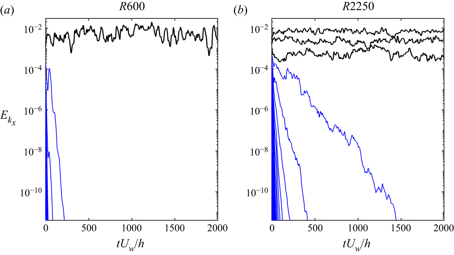
The supported space of RNL is determined by starting an RNL simulation from an initial DNS state that has energy in all the streamwise components. The  $N_a$ streamwise components that survive define the active RNL subspace, S, whereas the decaying components form the passive RNL subspace (cf. figure 12). Note that it is possible to also sustain RNL turbulence by constraining the RNL interactions to the streamwise-mean
 ${\boldsymbol {u}}_0$ with a selected single component of
 $\tilde {{\boldsymbol {u}}}$ that may or may not belong to
 $S$ (Bretheim et al. Reference Bretheim, Meneveau and Gayme2015). These simulations can even produce turbulence statistics that are closer to those of DNS from those obtained when no constraint is imposed on the RNL components, as shown in Bretheim et al. (Reference Bretheim, Meneveau and Gayme2015). However, when the constraint is removed and the other streamwise wavenumbers are allowed to freely evolve under the RNL dynamics, the supported space reverts to the active components
 $S$, defined above, and in that sense the active subspace of RNL is stable and unique.
Time evolution of the energy of the streamwise components in an RNL simulation initialized from a DNS state. This figure shows that the RNL turbulent state sustains only a few streamwise components. (a) The RNL simulation at  $R=600$ sustains only the
 $n=0$ (not shown) and the
 $n=1$ component (black). All other streamwise components decay exponentially to zero (blue). (b) The RNL simulation at
 $R=2250$ sustains only the
 $n=0$ (not shown) and the
 $n=1,2,3$ component (black), while all
 $n \geqslant 4$ streamwise components (blue) exponentially decay. The active RNL subspace includes
 $n=0,1$ at
 $R=600$ and the passive RNL subspace is all streamwise components
 $n\geqslant 2$, and
 $N_a=2$. The active RNL turbulence at
 $R=2250$ has
 $N_a=4$.

By performing simulations of the cases listed in table 1 we find that the RNL active subspace of  $R600$ has
 $N_a=2$ streamwise components, as RNL sustains only streamwise components
 $n=0,1$. The RNL active subspace of R1500 and R2250 has
 $N_a=4$, as only streamwise components
 $n=0,1,2,3$ are generically sustained in RNL. This is illustrated in figure 12 where we plot the time evolution of the energy of the streamwise components of
 $\tilde {{\boldsymbol {u}}}$ in an RNL simulation that has been initialized by a DNS state. The energy of all streamwise components with
 $n\geqslant 2$ at R600 and
 $n \geqslant 4$ at R2250 exponentially decay and the turbulent state sustains a streamwise varying flow
 $\tilde {{\boldsymbol {u}}}$ with streamwise component
 $n=1$ at R600 and
 $n=1,2,3$ at R2250.
Substantial overlap between the active subspaces of the DNS experiments and the corresponding active subspaces of RNL would suggest that the RNL dynamics govern the size of the active subspace and substantially controls the dynamics of synchronization. And indeed there is substantial overlap: the two active subspaces coincide at  $R=600$ as
 $N_a=2$ and
 $N_c=2$, while at
 $R=1500$ the active subspace of DNS has
 $N_c=5$ and that of RNL has
 $N_a=4$, and at
 $R=2250$ DNS has
 $N_c=6$ while RNL sustains
 $N_a=4$ streamwise Fourier components.
Interestingly though, those additional components of the active synchronization subspace of the DNS that are not sustained in RNL have the potential of synchronization, albeit within a stricter formulation of the synchronization problem. In this formulation we examine whether the selected  $n$th streamwise Fourier component of the flow
 $\boldsymbol{v}_n$ synchronizes to the
 $n$th streamwise Fourier component of the DNS
 ${\boldsymbol {u}}_n$, when coupled to all the other components of the DNS flow
 ${\boldsymbol {u}}_{n\prime} ={\boldsymbol {u}} -{\boldsymbol {u}}_n$. Here
 ${\boldsymbol {u}}$, as elsewhere, is the flow obtained in DNS, and
 $n\prime$ denotes cumulatively the indices of all the streamwise Fourier components included in the DNS except the index
 $n$. The dynamics of the component
 $\boldsymbol{v}_n$, which is starting from arbitrary initial conditions, is governed by the equation
 \begin{equation} \partial_t \boldsymbol{v}_n ={-}P_n \left ( ({\boldsymbol{u}}_{n\prime}+\boldsymbol{v}_n) \boldsymbol{\cdot} \boldsymbol{\nabla} ({\boldsymbol{u}}_{n\prime}+\boldsymbol{v}_n) - R^{{-}1} \Delta \boldsymbol{v}_n \right ), \end{equation}
with  $P_n$ the Leray projection to the
 $n$th streamwise Fourier component of the flow. The single streamwise-varying component
 $\boldsymbol{v}_n$ is then synchronizable if as time evolves it approaches the streamwise-varying component
 ${\boldsymbol {u}}_n$ of the DNS.
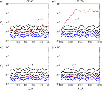
We performed experiments to examine the synchronizability of components  $n=3$ and
 $n=4$ at
 $R=1500$ and
 $R=2250$. The component
 $n=3$ is selected because it belongs to the active DNS subspaces at both Reynolds numbers and it is also the last member of the active RNL subspace at both Reynolds numbers. The component
 $n=4$ is selected because it is also a member of the active DNS subspace at both Reynolds numbers but it is not a member of the corresponding RNL active subspaces. It is in both cases the first member of their RNL passive subspace. We find that
 $\boldsymbol{v}_n$ with
 $n=3$ is not synchronizable at both Reynolds numbers (red dotted lines in figure 13a,b), while the
 $\boldsymbol{v}_n$ with
 $n=4$, which is passive in RNL but active in DNS, is synchronizable (red dotted line in figure 13c,d) under this new protocol. The significance of this result lies in the identification of the RNL active subspace as the source of chaotic dynamics, since only the trajectories of the active RNL components are inherently divergent. The association of this subspace with the energy extraction mechanism suggests that it is sustaining turbulence, and that it is exporting energy and pacing the other scales through nonlinear interactions.
Time series of the energy of the top streamwise harmonics in DNS (solid black lines denote the active RNL subspace and solid blue line denote the first passive streamwise components of the RNL subspace) at (a,c)  $R1500$ and at (b,d)
 $R2250$. In (a,b) it is shown that
 $\boldsymbol{v}_n$ (red dots) with
 $n=3$ does not synchronize to
 ${\boldsymbol {u}}_n$. In (c,d) it is shown that
 $\boldsymbol{v}_n$ (red dots) with
 $n=4$ does synchronize to
 ${\boldsymbol {u}}_n$. In these experiments the
 $\boldsymbol{v}_n$ component is initially set to zero. The
 $n=3$ component is selected because it is a part of the active subspace of the DNS and the last component in the active RNL subspace at both Reynolds numbers, while
 $n=4$ is in the active subspace of the DNS but is the first component of the passive RNL subspace.

5. Energy balances of the streamwise flow components
Energy transfers originating from the coherent large scales have been shown to influence the statistics of the turbulence that operates in the small scales of inhomogeneous flows (Thiesset et al. Reference Thiesset, Danaila and Antonia2014; Alves Portela et al. Reference Alves Portela, Papadakis and Vassilicos2020). This is amply demonstrated in wall-bounded turbulence in the RNL approximation, where the mean flow exercises control over the whole flow (Farrell & Ioannou Reference Farrell and Ioannou2017). Here, we use the streamwise mean decomposition of the flow  ${\boldsymbol {u}} = {\boldsymbol {u}}_0+\tilde {{\boldsymbol {u}}}$, used in RNL with
 ${\boldsymbol {u}}_0$ the instantaneous streamwise mean flow that has spanwise dependence, to study the energetics of the streamwise components of the active and passive subspaces of synchronization in the DNS examples. We examine the relative strength of the energy transfers to a given streamwise component from
 ${\boldsymbol {u}}_0$ (representing the transfer from this mean) and from other components of
 $\tilde {{\boldsymbol {u}}}$ (representing the transfer from nonlinear interactions).
To derive the energetics equation of the streamwise component,  ${\boldsymbol {u}}_n$, with wavelength
 $k_x=n \alpha$ and
 $n\geqslant 1$, we form the inner product of the equation governing
 $n$th streamwise component of
 $\tilde {{\boldsymbol {u}}}$, as follows:
 \begin{equation} \partial_t {\boldsymbol{u}}_n ={-}P_n \left ( {\boldsymbol{u}} \boldsymbol{\cdot} \boldsymbol{\nabla} {\boldsymbol{u}} - R^{{-}1} \Delta {\boldsymbol{u}} \right ), \end{equation}
with  ${\boldsymbol {u}}_n$ to obtain the equation for the energetics,
 \begin{equation} \partial_t E_{k_x} = \varPi_0 + \varPi_{k_x} - \epsilon_{k_x}. \end{equation}
Above,  $E_{k_x}= \langle {\boldsymbol {u}}_n, {\boldsymbol {u}}_n \rangle / 2$ is the energy density of the
 $n$th streamwise component of the flow, with angle brackets denoting the inner product integration over the flow domain;
 \begin{equation} \varPi_0={-} \langle {\boldsymbol{u}}_{n}, P_{n} \left ( {\boldsymbol{u}}_0 \boldsymbol{\cdot} \boldsymbol{\nabla} \tilde{{\boldsymbol{u}}} + \tilde{{\boldsymbol{u}}} \boldsymbol{\cdot} \boldsymbol{\nabla} {\boldsymbol{u}}_{0} \right )\rangle, \end{equation}
is the rate of energy transfer from  ${\boldsymbol {u}}_0$ to streamwise component
 $n$;
 \begin{equation} \varPi_{k_x} ={-} \langle {\boldsymbol{u}}_{n}, P_{n} \left ( \tilde{{\boldsymbol{u}}} \boldsymbol{\cdot} \boldsymbol{\nabla} \tilde{{\boldsymbol{u}}} \right )\rangle, \end{equation}
is the rate of energy transfer from the other scales to  $n$;
 \begin{equation} \epsilon_{k_x} ={-} \left\langle {\boldsymbol{u}}_{n},R^{{-}1} \Delta {\boldsymbol{u}}_{n} \right\rangle, \end{equation}
is the rate of dissipation.
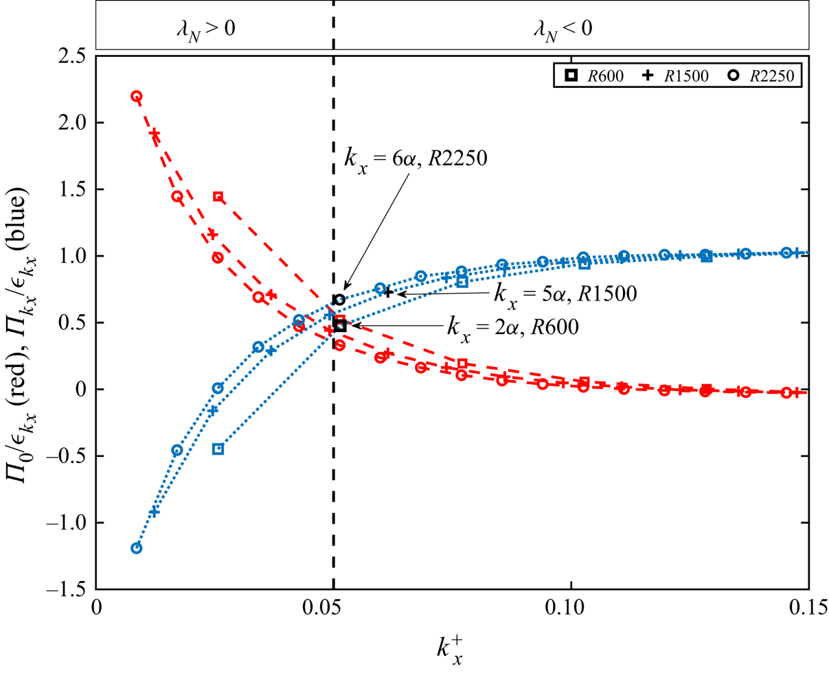
The terms of (5.2) are evaluated for every streamwise component, and the ratios of the time-averaged quantities,  $\varPi _0/ \epsilon _{k_x}$ and
 $\varPi _{k_x} / \epsilon _{k_x}$, are plotted as functions of the streamwise wavenumber scaled in viscous wall units,
 $k^+_x = n \alpha / R_{\tau }$, in figure 14. The scaling shows that the wavenumber
 $k_{xc}^+$ that demarcates the active and passive subspaces that can be synchronized (and is determined from the negative Lyapunov exponents in figure 5) collapses to a single wavenumber, corresponding to the critical wavelength
 $\ell _{xc}^+=130$. It is evident that the components that are sustained in RNL (with
 $k_x^+$ much smaller than
 $k_{xc}^+$) constitute the main sources of energy transfer from the mean flow. The gravest streamwise components of the passive subspace
 ${\boldsymbol {u}}_>$, which are
 $k_x=2\alpha$ for
 $R600$,
 $k_x=5\alpha$ for
 $R1500$ and
 $k_x=6\alpha$ for
 $R2250$, are located in a region of the spectrum where the linear production
 $\varPi _0$ has been reduced significantly and has been just overtaken by the
 $\varPi _{k_x}$ fluxes as the primary source of energy input. A similar switch between the nonlinear and viscous contributions to the energy flux that characterized the synchronizable scales was found by Clark Di Leoni et al. (Reference Clark Di Leoni, Mazzino and Biferale2020), which marked the passing from the inertial subrange to the dissipative scales.
Comparison of the ratio of the linear  $\varPi _0$ and nonlinear
 $\varPi _{k_x}$ transfer terms to dissipation,
 $\epsilon _{kx}$, as a function of the wavenumber
 $k_x^+=2 {\rm \pi}n / L_x^+$ of the
 $n$th streamwise Fourier component in wall units, for simulations at
 $R=600$,
 $R=1500$ and
 $R=2250$. All curves collapse to a single line with this scaling. The streamwise scale that renders
 ${\boldsymbol {u}}_>$ slave,
 $k_{xc}^+$, occurs on the vicinity of the negative Lyapunov exponent subspaces (the threshold between positive and negative values is denoted by the black dashed line at
 $k_x^+=0.05$) and is indicated with black markers (square for
 $R=600$, cross for
 $R=1500$ and circle for
 $R=2250$).

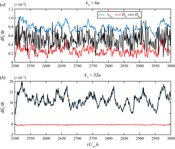
Time series of the three terms in (5.2) are plotted in figure 15 for  $n=6$ and
 $n=32$ for an
 $R=2250$ simulation. It is remarkable that scales as large as
 $130$ wall units that receive energy both from the mean flow and from nonlinear interaction, like the
 $n=6$ component shown in figure 15(a), are slave to the larger-scale flow. An increase in
 $k^+_x$ shifts the balance of the components in the passive subspace to an equilibrium between
 $\varPi _{k_x}$ and
 $\epsilon _{k_x}$ at every time instance (cf. the black and blue lines shown in figure 15b), indicating that dissipative dynamics eventually fully govern this part of the spectrum.
Time series of the energetic terms in (5.2) of an  $R2250$ simulation for (a)
 $k_x=6\alpha$ and (b)
 $k_x=32\alpha$. Shown are the energy transfer to
 $k_x$ from the mean flow
 $\varPi _0$ (red), the energy dissipation rate
 $-\epsilon _{kx}$ (blue) and the total energy transfer by the nonlinear interactions,
 $\varPi _{kx}$ (black).

The resulting negative Lyapunov exponents that indicate that the subspace  ${\boldsymbol {u}}_>$ is synchronizable, coincide with the increased nonlinear flux terms, which exert control from the energy extracting scales to the small scales, and the components with higher streamwise wavenumbers, which are more dissipative. This implies that the larger-scale flow organizes the nonlinear transfers to the smaller scales and that nonlinear interaction from the smaller to the larger scales within the passive subspace is not able to dictate the evolution.
6. Discussion
We have performed a series of synchronization experiments in wall-bounded turbulent Couette flows, where we employ a streamwise Fourier decomposition to split the flow into an active subspace  ${\boldsymbol {u}}_<$ and a passive subspace
 ${\boldsymbol {u}}_>$ according to a critical harmonic
 $N_c$. We can determine
 $N_c$ by calculating the Lyapunov exponent of perturbations
 ${\boldsymbol {u}}\prime_>$ to the time-dependent flow
 ${\boldsymbol {u}}_>+{\boldsymbol {u}}_<$ and by requiring that
 $N_c$ is the first component with
 $\lambda _{N_c} <0$. Our results show that the components
 ${\boldsymbol {u}}_<$ that lead to a complete reconstruction of the dynamical state of the flow are comprised of a small number of streamwise Fourier components. This finding confines the attractor on
 ${\boldsymbol {u}}_<$ and, therefore, defines the projection of the equations which are dynamically significant in each flow. Interestingly, the fundamentally chaotic behaviour of this attractor appears to be associated with the components that are maintained in the parametrically active RNL subspace, which is primarily driven by the energy extraction from the streamwise-mean component.
We chose the streamwise Fourier decomposition because in this decomposition the basis functions have dynamical significance. They reflect the dynamics of the self-sustaining process in the buffer layer. This is demonstrated with clarity in RNL (or QL) turbulence in which the interaction of the streamwise-mean with a few streamwise-varying Fourier components supports a realistic state of wall-bounded turbulence (Farrell & Ioannou Reference Farrell and Ioannou2012; Bretheim et al. Reference Bretheim, Meneveau and Gayme2015; Farrell & Ioannou Reference Farrell and Ioannou2017; Farrell et al. Reference Farrell, Gayme and Ioannou2017). A decomposition based on the eigenfunctions of the Stokes operator (cf. Ladyzhenskaya Reference Ladyzhenskaya1975) or on the three-dimensional Fourier basis (cf. Yoshida et al. Reference Yoshida, Yamaguchi and Kaneda2005; Lalescu et al. Reference Lalescu, Meneveau and Eyink2013; Clark Di Leoni et al. Reference Clark Di Leoni, Mazzino and Biferale2020) does not have such dynamical significance at the anisotropic energy bearing scales in wall-bounded flows.
Associated with the critical truncation at streamwise component  $N_c$ that leads to synchronization is the critical length scale which is approximately equal to
 $\ell _x^+=130$ wall units for the three different Reynolds numbers studied here. The scaling with wall units suggests that the active subspaces involve states that emerge near the wall. This conjecture implies that the wavelength cutoff of
 ${\boldsymbol {u}}_>$ could also characterize the medium
 $R_{\tau }$ experiments of Nikitin (Reference Nikitin2018), since the Lyapunov exponent of the total flow exhibits a form of universality as it collapses to a single value when scaled with wall units. The cutoff length scale coincides also with the peaks found by Nikitin (Reference Nikitin2018) in the spectra of the vertical velocity
 $v$ and spanwise velocity
 $w$ at
 $y^+=14$ for the Lyapunov vector of the total flow at
 $R_{\tau }=391$. Interestingly, once we restrict the streamwise length scale of the subspaces below this peak, the subspaces are stabilized.
A comparison of  $\ell _{xc}^+$ can be made with the length scales attributed to the Kolmogorov dissipation range. Translating
 $\ell _{xc}^+=130$ into Kolmogorov lengths, defined as
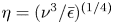 $\eta = (\nu ^3/ \bar {\epsilon } )^{(1/4)}$ (for
 $R2250$ the time-averaged dissipation per unit of mass,
 $\bar {\epsilon }$, equals
 $0.0035U_w^3/h$), we find that the critical
 $\ell _x^+ \approx 77\eta$ is above the assumed dissipation subrange cutoff of
 $\ell \approx 60 \eta$. This implies, if these estimates obtained from our low Reynolds number simulations are also relevant at higher Reynolds numbers, that a small portion of the motions that belong to the inertial subrange of the spectrum can be synchronized by the larger scales. The synchronization experiments in IHT (Yoshida et al. Reference Yoshida, Yamaguchi and Kaneda2005; Lalescu et al. Reference Lalescu, Meneveau and Eyink2013; Clark Di Leoni et al. Reference Clark Di Leoni, Mazzino and Biferale2020; Vela-Martín Reference Vela-Martín2021) have recovered a cutoff wavenumber for synchronization between
 $k \eta = 0.15 - 0.2$ (
 $\ell _c$ between
 $30 \eta$ and
 $40\eta$. These values correspond to the critical values quoted by Yoshida et al. (Reference Yoshida, Yamaguchi and Kaneda2005) and Lalescu et al. (Reference Lalescu, Meneveau and Eyink2013) as these authors define the critical wavenumber as
 $k={\rm \pi} / \ell _c$ instead of
 $k= 2 {\rm \pi}/\ell _c$. When we scale the growth rates and wavenumbers in the same units, we find that the length scale of the synchronization threshold in our channel flows occurs at
 $k_x \eta \approx 0.082$, at length scales that are twice as large. Comparisons between IHT and rotating three-dimensional turbulence have shown that the presence of large-scale structure in rotating turbulence reduces significantly the amount of necessary input to achieve synchronization (Clark Di Leoni et al. Reference Clark Di Leoni, Mazzino and Biferale2020). Such large-scale structures are also prevalent in the wall-bounded flows studied in this work, which we consider the main cause for the difference found on the length scale of the synchronizable scales.
The critical streamwise length scale for synchronization is also in broad agreement with the streamwise resolution estimates that Wang & Zaki (Reference Wang and Zaki2021) obtained in order to accurately reconstruct the flow state in plane Poiseuille turbulence from observations. This is to be expected, because successful assimilation of the full flow requires that the unobserved small scales be synchronizable. This work also suggests that the time scale of the assimilation is set by the Lyapunov exponent  $\lambda _N$, with the
 $N$ corresponding to the threshold scale. Apart from flow reconstruction applications, considerable effort has been devoted to developing modelling approaches that rely on machine learning techniques (Ling & Templeton Reference Ling and Templeton2015; Tracey, Duraisamy & Alonso Reference Tracey, Duraisamy and Alonso2015; Gamahara & Hattori Reference Gamahara and Hattori2017; Lozano-Durán & Bae Reference Lozano-Durán and Bae2020). Although data-driven turbulence modelling has succeeded in reproducing certain features of the turbulent dynamics (e.g. Yang et al. Reference Yang, Zafar, Wang and Xiao2019; Inubushi & Goto Reference Inubushi and Goto2020), challenges of building reliable data-driven models have proved significant and it is believed that physical knowledge of the flow dynamics, such as the dependence of the streamwise small scales from the large ones obtained in this work, could prove beneficial in the future development of machine learning modelling (cf. Duraisamy, Iaccarino & Xiao Reference Duraisamy, Iaccarino and Xiao2019).
Synchronization is not restricted to IHT and wall-bounded turbulence. In the works of Alves Portela et al. (Reference Alves Portela, Papadakis and Vassilicos2020) and Thiesset et al. (Reference Thiesset, Danaila and Antonia2014), the small-scale component that is hypothesized to describe the stochastic turbulence was found to be influenced by the time-dependent large-scale coherent structures of the flow. Alves Portela et al. (Reference Alves Portela, Papadakis and Vassilicos2020) also identified a range of length scales where the components of the energetics are maintained in an equilibrium between dissipation and the nonlinear fluxes. We can, therefore, assume that the passive subspace  ${\boldsymbol {u}}_>$ that we defined in this work is related to the stochastic component and the highly influenced statistics found in those studies are a consequence of the synchronization imposed to
 ${\boldsymbol {u}}_>$ from the coherent motions of the active subspace, identified here with
 ${\boldsymbol {u}}_<$.
7. Conclusions
Synchronization in wall-bounded turbulent Couette flows occurs when an active subspace  ${\boldsymbol {u}}_<$ of the solution is sufficient to reconstruct a passive subspace
 ${\boldsymbol {u}}_>$. Similar arguments are used in uniqueness theorems of solutions to define a finite-dimensional global attractor of the Navier–Stokes equations. As such, we argue that the equations governing
 ${\boldsymbol {u}}_<$ fully determine the dynamics on the turbulent attractor. Using a streamwise Fourier decomposition, we demonstrated that in plane Couette turbulence at low Reynolds numbers the synchronizable subspaces
 ${\boldsymbol {u}}_>$ are comprised by all the Fourier components with streamwise wavelengths shorter than
 $\ell _x^+=130$.
The existence of this threshold was verified in a series of experiments at low Reynolds numbers and its connection with the top Lyapunov vector implies that the critical wavelength scaling holds for flows where this vector is concentrated in the buffer layer region (which has been shown by Nikitin (Reference Nikitin2018) to apply for the top Lyapunov vector in flows up to  $R_{\tau }=586$), where the large-scale structure is comprised of rolls and streaks. Evidence pointing to synchronization phenomena has also been found in other inhomogeneous flow configurations, where the statistics and structure functions of the small-scale fluctuations are strongly influenced by the large-scale coherent component of the flow (Thiesset et al. Reference Thiesset, Danaila and Antonia2014; Alves Portela et al. Reference Alves Portela, Papadakis and Vassilicos2020). The state estimation results of Wang & Zaki (Reference Wang and Zaki2021) for plane Poiseuille turbulence can also be attributed to synchronization.
The active subspace  ${\boldsymbol {u}}_<$ spans only a fraction of the streamwise spectrum but the energy contained in these components is a significant portion of the total kinetic energy, as was shown to be the case in IHT (Henshaw et al. Reference Henshaw, Kreiss and Yström2003; Yoshida et al. Reference Yoshida, Yamaguchi and Kaneda2005; Clark Di Leoni et al. Reference Clark Di Leoni, Mazzino and Biferale2020). The components of
 ${\boldsymbol {u}}_<$ are mainly responsible for the energy extraction from the mean flow. We also show that stricter synchronization experiments detect the modes that comprise the active RNL subspace of the flow, suggesting that the active RNL subspace captures the source of chaotic dynamics in turbulent flows.
Although the passive subspace  ${\boldsymbol {u}}_>$ of the solution is unique, it cannot be neglected from numerical calculations, as truncating the streamwise harmonics to an
 $N_c$ wavenumber are severe and are known to reduce the accuracy of numerical solutions. Instead, since
 ${\boldsymbol {u}}_>$ is a function of
 ${\boldsymbol {u}}_<$, it is possible that aiming to implement this information into current modelling efforts could provide significantly accurate models for the small scales of the flow.
Supplementary movies
Supplementary movies are available at https://doi.org/10.1017/jfm.2021.1054.
Funding
M.-A.N. gratefully acknowledges the support of the Hellenic Foundation for Research and Innovation (HFRI) and the General Secretariat for Research and Technology (GSRT), under the HFRI PhD Fellowship grant 1718/14518. We gratefully acknowledge the comments of the three anonymous reviewers and discussions with B. Farrell and N. Constantinou.
Declaration of interests
The authors report no conflict of interest.