1. Introduction
In Hall magnetohydrodynamic (HMHD) turbulence, ion and electron motions become distinct at scales comparable to or smaller than the ion inertial length. This distinction is described by the Hall term in the generalised Ohm’s law (Galtier Reference Galtier2016). The HMHD model is thus essential for plasma phenomena such as collisionless magnetic reconnection in the magnetosphere and solar corona (Bhattacharjee Reference Bhattacharjee2004; Dorelli et al. Reference Dorelli, Glocer, Collinson and Tóth2015), kinetic-scale turbulence and energy cascades in the solar wind (Galtier Reference Galtier2006; Gary & Smith Reference Gary and Smith2009), the formation of sharp current sheets and whistler-wave activity (Galtier Reference Galtier2016) and the evolution of magnetised accretion disks and protostellar collapse (Marchand et al. Reference Marchand, Tomida, Commerçon and Chabrier2019; Wurster, Bate & Bonnell Reference Wurster, Bate and Bonnell2021).
In the solar corona, strongly helical magnetic fields undergo collisionless reconnection, contributing to transient eruptive phenomena such as coronal mass ejections, which in turn can enhance the solar wind flux (Faganello, Califano & Pegoraro Reference Faganello, Califano and Pegoraro2008; Servidio et al. Reference Servidio, Matthaeus, Shay, Cassak and Dmitruk2009; Ebrahimi & Raman Reference Ebrahimi and Raman2015; Wan et al. Reference Wan, Matthaeus, Roytershteyn, Karimabadi, Parashar, Wu and Shay2015; Sun et al. Reference Sun, Yang, Lu, Lu, Wan and Wang2022). The solar wind is a continuous flow of charged particles, mainly electrons and protons. Propagating at speeds from 200 to 800 km s−1, it carries a interplanetary magnetic field throughout the heliosphere (Marino & Sorriso-Valvo Reference Marino and Sorriso-Valvo2023). Politano & Pouquet (Reference Politano and Pouquet1998) extended the von Kármán–Howarth (vKH) relation (De Karman & Howarth Reference De Karman and Howarth1938; Kolmogorov Reference Kolmogorov1941) to magnetohydrodynamic (MHD) turbulence. This relation has since been applied to in situ measurements to characterise the turbulent properties of the solar wind (Sorriso-Valvo et al. Reference Sorriso-Valvo, Marino, Carbone, Noullez, Lepreti, Veltri, Bruno, Bavassano and Pietropaolo2007; Marino et al. Reference Marino, Sorriso-Valvo, Carbone, Veltri, Noullez and Bruno2011, Reference Marino, Sorriso-Valvo, D’Amicis, Carbone, Bruno and Veltri2012). In addition to these vKH-based analyses, solar wind turbulence has been studied in terms of intermittency and current sheets (Veltri & Mangeney Reference Veltri and Mangeney1999; Bruno et al. Reference Bruno, Carbone, Primavera, Malara, Sorriso-Valvo, Bavassano and Veltri2004, Reference Bruno, Carbone, Chapman, Hnat, Noullez and Sorriso-Valvo2007; Greco et al. Reference Greco, Matthaeus, Servidio, Chuychai and Dmitruk2009; Osman et al. Reference Osman, Matthaeus, Wan and Rappazzo2012; Sorriso-Valvo et al. Reference Sorriso-Valvo, Marino, Lijoi, Perri and Carbone2015), as well as directional alignments and cellular structuring (Osman et al. Reference Osman, Wan, Matthaeus, Breech and Oughton2011). The resulting magnetic energy spectrum follows a
 $k^{-5/3}$
Kolmogorov scaling against the wavenumber
 $k$
, whereas the kinetic energy spectrum exhibits a
 $k^{-3/2}$
Iroshnikov–Kraichnan scaling (Alexakis Reference Alexakis2013), in agreement with solar wind observations (Podesta, Roberts & Goldstein Reference Podesta, Roberts and Goldstein2007; Salem et al. Reference Salem, Mangeney, Bale and Veltri2009; Schekochihin Reference Schekochihin2022). Under a strong guiding field, the perpendicular magnetic spectrum transits from
 $k_\perp ^{-5/3}$
to
 $k_\perp ^{-3/2}$
(Goldreich & Sridhar Reference Goldreich and Sridhar1997; Boldyrev Reference Boldyrev2005, Reference Boldyrev2006; Chen et al. Reference Chen2020).
In solar wind turbulence, geometric features related to the alignment of the velocity, magnetic field and magnetic potential can be measured through several helicity functions (kinetic, magnetic and cross-helicity) (Galtier Reference Galtier2016). In MHD or HMHD turbulence, besides energy, magnetic helicity is also an inviscid invariant (Elsasser Reference Elsasser1956; Woltjer Reference Woltjer1958), which quantifies the linkage and twist of magnetic field lines (Galtier Reference Galtier2016). Due to the conservation of energy and its relation to magnetic helicity, magnetic helicity has been found to be inversely cascaded toward large scales (Frisch et al. Reference Frisch, Pouquet, Léorat and Mazure1975; Alexakis & Biferale Reference Alexakis and Biferale2018). If driven at small scales, the inverse-cascade results in the formation of large-scale magnetic structures, which have been linked to the
 $\alpha$
-dynamo action (Müller et al. Reference Müller, Malapaka and Busse2012; Richner et al. Reference Richner, Bodner, Bongard, Fonck, Nornberg and Reusch2022). Linkmann & Dallas (Reference Linkmann and Dallas2017) explored this inverse cascades using triad-interaction analysis in the Fourier helical decomposition framework, identifying key mechanisms such as the stretch–twist–fold dynamics and small-scale dynamo activity. Aluie & Eyink (Reference Aluie and Eyink2010) introduced the filtering approach to MHD turbulence and found that energy cascades are primarily governed by local interactions, whereas magnetic helicity cascades are dominated by non-local triads. Bian & Aluie (Reference Bian and Aluie2019) further found the decoupling between the magnetic and kinetic energy cascades. Besides magnetic helicity, cross-helicity also plays a significant role in the turbulent cascades (Galtier Reference Galtier2016). The cross-helicity is defined by the dot product of the velocity and magnetic fields (
 $\boldsymbol v \boldsymbol{\cdot }\boldsymbol b$
), while interscale cascades are associated with the cross-product (
 $\boldsymbol v \times \boldsymbol b$
). As the cross-helicity increases, the velocity and magnetic fields align with each other, leading to the suppression of turbulent cascades. Boldyrev (Reference Boldyrev2005, Reference Boldyrev2006) identified this dynamical alignment as energy transfers to smaller scales in the presence of a guiding magnetic field. This alignment results in a scale-dependent reduction of the nonlinear interaction strength, yielding the
 $k_\perp ^{-3/2}$
Iroshnikov–Kraichnan spectrum (Boldyrev Reference Boldyrev2006; Chandran, Schekochihin & Mallet Reference Chandran, Schekochihin and Mallet2015). This spectrum has been supported by both numerical simulations and solar wind observations (Mason, Cattaneo & Boldyrev Reference Mason, Cattaneo and Boldyrev2008; Perez et al. Reference Perez, Mason, Boldyrev and Cattaneo2012; Chen et al. Reference Chen2020). These spectral results provide indirect evidence of cascade suppression by cross-helicity. More directly, solar wind observations have showed that elevated cross-helicity is associated with the reduced forward energy cascade (Smith et al. Reference Smith, Stawarz, Vasquez, Forman and MacBride2009) and the suppressed turbulence intensity (Marino et al. Reference Marino, Sorriso-Valvo, D’Amicis, Carbone, Bruno and Veltri2012).
At scales approaching the ion inertial length, the ideal MHD framework becomes inadequate, and the HMHD model provides a more suitable description of the underlying dynamics. Galtier (Reference Galtier2008) first extended the vKH relation for energy cascades to the HMHD regime. Using numerical data, Ferrand et al. (Reference Ferrand, Galtier, Sahraoui, Meyrand, Andrés and Banerjee2019) then confirmed the equivalence of several expressions of the vKH relation for energy cascades (Banerjee & Galtier Reference Banerjee and Galtier2016a ; Hellinger et al. Reference Hellinger, Verdini, Landi, Franci and Matteini2018; Ferrand et al. Reference Ferrand, Galtier, Sahraoui, Meyrand, Andrés and Banerjee2019). Banerjee & Galtier (Reference Banerjee and Galtier2016b ) further derived exact relations for the magnetic helicity under the assumption of homogeneity. Wang & Chkhetiani (Reference Wang and Chkhetiani2023) established the local vKH relations for the magnetic helicity in both inviscid electron and HMHD turbulence, revealing a Four-thirds law analogous to that for the energy. In a two-dimensional HMHD simulation, Camporeale et al. (Reference Camporeale, Sorriso-Valvo, Califano and Retinò2018) quantified the relationship between scale-to-scale energy transfers and coherent structures, showing that 50 % of the energy transfer occurs in only 25 % of the spatial domain. Kuzzay, Alexandrova & Matteini (Reference Kuzzay, Alexandrova and Matteini2019) studied the local Kármán–Howarth–Moin relation and highlighted the quasi-one-dimensional or quasi-two-dimensional structures with high cascade rates. Manzini et al. (Reference Manzini, Sahraoui, Califano and Ferrand2022) employed the filtering approach to investigate how magnetic reconnection sites contribute to energy dissipation in HMHD turbulence. Additionally, in numerical simulations, Mininni, Gómez & Mahajan (Reference Mininni, Gomez and Mahajan2005) revealed the enhanced growth of large-scale magnetic fields attributed to Hall effects. However, due to the limitations of numerical configurations, the specific and quantitative impact of Hall effects on inverse cascades remains uncertain. Moreover, observational evidence and analysis of the coupling between inverse cascades and Hall effects in solar wind turbulence are still scarce.
In this study, through direct numerical simulations and near-Sun solar wind observations, we investigate the Hall effects on inverse cascades. Our findings reveal that small-scale Hall effects can significantly enhance the magnetic field at larger scales. This enhancement is attributed to the reduced cascade efficiency caused by non-conservative cross-helicity. The paper is organised as follows. We present the details of the simulations and numerical results in § 2. Next, in § 3, the numerical findings are verified using solar wind data from the Parker Solar Probe. Finally, conclusions are presented in § 4.
2. Numerical simulations
2.1. Numerical set-up
The governing equations for the velocity
 $\boldsymbol v$
and the magnetic field
 $\boldsymbol b$
are written respectively as follows (Müller et al. Reference Müller, Malapaka and Busse2012; Marino & Sorriso-Valvo Reference Marino and Sorriso-Valvo2023):
 \begin{equation} \begin{aligned} \partial _t {\boldsymbol v} & = -({\boldsymbol v} \boldsymbol \cdot {\boldsymbol{\nabla }} ){\boldsymbol v} -{ \boldsymbol{\nabla }} p+{\boldsymbol j}\times {\boldsymbol b} +\lambda \Delta ^{-1}{\boldsymbol v}-\nu (-\varDelta )^\alpha {\boldsymbol v}+{\boldsymbol f_{\!v}}, \nonumber\\ \partial _t {\boldsymbol b} & = \boldsymbol{\nabla }\times ({\boldsymbol U}\times {\boldsymbol b}) +\lambda _{b}\Delta ^{-1}{\boldsymbol b}-\eta (-\varDelta )^\alpha {\boldsymbol b} +{\boldsymbol f_{\!b}},\\ \end{aligned} \end{equation}
where
 $\boldsymbol{\nabla }\boldsymbol{\cdot }{\boldsymbol v}=0$
,
 $\boldsymbol{\nabla }\boldsymbol{\cdot }{\boldsymbol b}=0$
,
 $p$
is the fluid pressure,
 ${\boldsymbol U}={\boldsymbol v}-d_I{\boldsymbol j}$
,
 ${\boldsymbol j}=\boldsymbol{\nabla }\times {\boldsymbol b}$
is the current density,
 $d_I$
is the ion inertial length,
 $\boldsymbol f_{\!v}$
and
 $\boldsymbol f_{\!b}$
are the forcing terms,
 $\lambda$
and
 $\lambda _{b}$
are hypo-viscous coefficients for the velocity and magnetic fields, respectively,
 $\nu$
and
 $\eta$
are the kinematic viscosity and the magnetic diffusivity, respectively, and
 $\alpha$
is the hyper-viscous order.
The code used in this analysis solves the governing equations using the Fourier series in periodic boxes and is developed based on the code for hydrodynamic turbulence (Yan et al. Reference Yan, Li, Yu, Wang and Chen2020; Hu et al. Reference Hu, Li and Yu2022). Isotropic white noise forcing schemes (
 ${\boldsymbol f}_{\!v}$
and
 ${\boldsymbol f}_{\!b}$
) are applied to the simulation;
 ${\boldsymbol f}_{\!v}$
is non-helical, while
 ${\boldsymbol f}_{\!b}$
is fully helical
 \begin{equation} \frac {{\boldsymbol f}_{\!b} \boldsymbol{\cdot }(\boldsymbol{\nabla }\times {\boldsymbol f}_{\!b})}{|{\boldsymbol f}_{\!b} || (\boldsymbol{\nabla }\times {\boldsymbol f}_{\!b})|}=1 . \end{equation}
These forcing schemes only inject magnetic helicity artificially and do not inject any kinetic or cross-helicity. For HMHD cases, due to the short time scale of the Hall effects, we use the split time step for the velocity and magnetic fields to speed up the calculations (Beresnyak Reference Beresnyak2018).
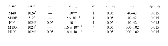
Five numerical cases are discussed in this paper. The computational parameters are listed in table 1. Cases M40, M40E and M100 are MHD simulations with different forcing wavenumbers
 $k_f$
, while H40 and H100 are HMHD simulations. All five cases (H40, M40, H100, M100 and M40E) are initially evolved on a
 $512^3$
grid until both the magnetic helicity and total energy reach statistically steady states. Except for M40E, the simulations are then interpolated onto a
 $1024^3$
grid and further evolved for at least
 $12.4\,T_0$
, where the eddy turnover time is defined as
 $T_0 = 2\pi / [k_f \sqrt { \langle v_i v_i+b_i b_i \rangle / 3}]$
. All statistical results reported in this study are averaged over a period of no less than
 $2.0 \,T_0$
.
Parameters of the computational configurations. Here,
 $d_I$
is the ion inertial length,
 $\nu$
and
 $\eta$
are the kinematic viscosity and the magnetic diffusivity, respectively,
 $\alpha$
is the hyper-viscous order,
 $\lambda$
and
 $\lambda _{b}$
are hypo-viscous coefficients for the velocity and magnetic fields, respectively,
 $k_f$
is the forcing wavenumber and
 $\varepsilon _{v}$
and
 $\varepsilon _{b}$
are injection rates of kinetic and magnetic energy, respectively.

2.2. Numerical results
The spectra of kinetic energy (
 $E_{v}(k)$
), magnetic energy (
 $E_{b}(k)$
) and magnetic helicity (
 $H_M(k)$
) are defined by
 \begin{equation} \begin{aligned} &E_{v}(k)=\sum _{|{\boldsymbol k}|=k}{\textrm{Re}} \{ \hat {\boldsymbol v}({\boldsymbol k})\boldsymbol{\cdot }\hat {\boldsymbol v}^\ast ({\boldsymbol k})\}/2,\\ &E_{b}(k)=\sum _{|{\boldsymbol k}|=k}{\textrm{Re}} \{ \hat {\boldsymbol b}({\boldsymbol k})\boldsymbol{\cdot }\hat {\boldsymbol b}^\ast ({\boldsymbol k})\}/2,\\ &H_M(k)=\sum _{|{\boldsymbol k}|=k}{\textrm{Re}} \{ \hat {\boldsymbol a}({\boldsymbol k})\boldsymbol{\cdot }\hat {\boldsymbol b}^\ast ({\boldsymbol k})\},\\ \end{aligned} \end{equation}
where
 $\hat {\boldsymbol \cdot}$
represents the values in spectral space, the superscript
 $\ast$
represents the conjugate value,
 $\hat {\boldsymbol a} ({\boldsymbol k})=[\textrm {i}\boldsymbol{k}\times \hat {\boldsymbol{b}}({\boldsymbol k})]/|\boldsymbol{k}|^2$
is the magnetic potential,
 $\textrm {i}$
denotes the imaginary unit,
 ${\textrm{Re}}$
and
 $\textrm{Im}$
represent the real and imaginary parts of a complex value.
Spectra. (a) Kinetic energy spectrum
 $E_{v}(k)$
. (b) Magnetic energy spectrum
 $E_{b}(k)$
. (c) Magnetic helicity spectrum
 $H_M(k)$
. Here,
 $L/d_I$
is the ion inertial scale
 $d_I$
normalised by the computational domain scale
 $L$
.

Evolution of
 $H_M(k)k^{10/3}$
for M40E. Time increases along the arrow, and the values are given in the legend after normalisation by the eddy turnover time
 $T_0$
.

The spectra
 $E_{v}(k)$
,
 $E_{b}(k)$
and
 $H_M(k)$
are given in figure 1. The kinetic energy spectra
 $E_{v}(k)\sim k^{-3/2}$
, the magnetic energy spectra
 $E_{b}(k)\sim k^{-5/3}$
and the magnetic helicity spectra
 $H_M(k)\sim k^{-8/3}\sim E_{b}(k)/k$
, implying that the magnetic field is fully helical. In comparison, only a slope around
 $k^{-10/3}$
has been reported based on unsteady numerical simulations with hyper-viscosity (Müller et al. Reference Müller, Malapaka and Busse2012; Linkmann & Dallas Reference Linkmann and Dallas2017). Therefore, an evolutionary case M40E with a relatively lower grid resolution of
 $512^3$
is given here for verification. The evolution of the magnetic helicity spectra
 $H_M(k)$
is given in figure 2. The time is normalised by the eddy turnover time
 $T_0$
. As time evolves,
 $H_M(k) \sim k^{-10/3}$
when
 $t/T_0\in [8.33,41.7]$
, but
 $H_M(k) \sim k^{-8/3}$
at
 $t/T_0=104.0$
. The comparison further verifies the validity of our data.
In figure 1, a comparison between the MHD and HMHD cases shows that Hall effects enhance large-scale magnetic energy and helicity by nearly an order of magnitude. This indicates that the ion-scale dynamics continues to influence the magnetic field at larger scales, which is the main finding of this study.
To understand the mechanism behind the magnetic field enhancement, the cascade rates should be measured. The filtering approach (Aluie & Eyink Reference Aluie and Eyink2010; Aluie Reference Aluie2017; Camporeale et al. Reference Camporeale, Sorriso-Valvo, Califano and Retinò2018; Manzini et al. Reference Manzini, Sahraoui, Califano and Ferrand2022) is employed to examine the scale-dependent features of the cascades. Different filter functions have been shown to yield qualitatively consistent results (Kuzzay et al. Reference Kuzzay, Alexandrova and Matteini2019; Yan et al. Reference Yan, Li, Yu, Wang and Chen2020). The fourth-order Butterworth filter (Camporeale et al. Reference Camporeale, Sorriso-Valvo, Califano and Retinò2018) is used in this study. The interscale flux for kinetic energy cascades can be written as
 \begin{equation} \begin{aligned} \widetilde \varPi _{\textit{Ev}}=-\epsilon _{\textit{ijk}}\left [\tilde v_i \tau _{jk}({\boldsymbol v},{\boldsymbol{\omega } }) +\tilde v_i \tau _{jk}({\boldsymbol j},{\boldsymbol{b} }) \right]\!, \end{aligned} \end{equation}
where the vorticity
 $\boldsymbol{\omega }=\boldsymbol{\nabla }\times \boldsymbol{v}$
,
 $\epsilon _{\textit{ijk}}$
is the Levi-Civita symbol,
 ${\boldsymbol \tau }_{\textit{ij}}({\boldsymbol p},{\boldsymbol q} )=\widetilde {{ p_i q_j}}-\widetilde {{p}_i }\widetilde {{q}_j }$
and the superscript
 $\widetilde {\boldsymbol{\cdot }}$
represents a filtered quantity. The interscale flux for the magnetic energy cascades can be written as
 \begin{equation} \begin{aligned} \widetilde \varPi _{Eb1}&=-\epsilon _{\textit{ijk}}\tilde j_i \tau _{jk}({\boldsymbol v},{\boldsymbol{b} }),\\ \widetilde \varPi _{Eb2}&=\epsilon _{\textit{ijk}}d_I\tilde j_i \tau _{jk}({\boldsymbol j},{\boldsymbol b}),\\ \widetilde \varPi _{Eb}&=\widetilde \varPi _{Eb1}+\widetilde \varPi _{Eb2}. \end{aligned} \end{equation}
The interscale flux for magnetic helicity cascades can be written as
 \begin{equation} \begin{aligned} \widetilde \varPi _{\textit{HM}1}&=-2\epsilon _{\textit{ijk}}\tilde b_i \tau _{jk}({\boldsymbol v},{\boldsymbol b}),\\ \widetilde \varPi _{\textit{HM}2}&=2\epsilon _{\textit{ijk}}d_I\tilde b_i \tau _{jk}({\boldsymbol j},{\boldsymbol b}),\\ \widetilde \varPi _{\textit{HM}}&=\widetilde \varPi _{\textit{HM}1}+\widetilde \varPi _{\textit{HM}2}. \end{aligned} \end{equation}
Here,
 $\widetilde \varPi _{Eb1}$
and
 $\widetilde \varPi _{\textit{HM}1}$
are the MHD terms, while
 $\widetilde \varPi _{Eb2}$
and
 $\widetilde \varPi _{\textit{HM}2}$
are the Hall terms.
Fluxes versus the filter width
 $\varDelta$
. Here,
 $\varDelta$
is normalised by the computational domain scale
 $L$
. (a,b) Kinetic energy fluxes for (a) H40 and M40, (b) H100 and M100. (c,d) Magnetic energy fluxes for (c) H40 and M40, (d) H100 and M100. (e,f) Magnetic helicity fluxes for (e) H40 and M40, (f) H100 and M100. Solid lines: HMHD cases; dashed lines: MHD cases.

Figures 3 (a) and 3(b) show the kinetic energy fluxes
 $\langle \widetilde \varPi _{\textit{Ev}} \rangle$
, where
 $\langle \boldsymbol{\cdot } \rangle$
represents the ensemble average. The inverse cascades of
 $\langle \widetilde \varPi _{\textit{Ev}} \rangle$
are negligible, and the Hall effects have minimal impact on the kinetic energy fluxes. The magnetic energy flux
 $\langle \widetilde \varPi _{Eb} \rangle$
and its decomposition are shown in figures 3 (c) and 3(d). As shown, most magnetic energy cascades forward toward small scales. Regardless of the forcing wavenumber, the Hall term
 $\langle \widetilde {\varPi }_{Eb2} \rangle$
dominates at small scales (
 $\varDelta /L \lessapprox 10^{-2}$
), which is attributed to its higher-order nature. Weak inverse cascades appear and are linked to the
 $\alpha$
-dynamo action (Müller et al. Reference Müller, Malapaka and Busse2012; Linkmann & Dallas Reference Linkmann and Dallas2017; Pouquet et al. Reference Pouquet, Rosenberg, Stawarz and Marino2019). Hall effects also have little influence on the inverse-cascade rates of magnetic energy. Figures 3 (e) and 3(f) show the mean magnetic helicity flux
 $\langle \widetilde {\varPi }_{\textit{HM}} \rangle$
and its decomposition. The component
 $\langle \widetilde {\varPi }_{\textit{HM}1} \rangle$
is dominant, with most magnetic helicity cascading inversely toward large scales.
Hall effects have a minimal impact on the inverse cascades shown in figure 3, but strongly enhance the large-scale velocity and magnetic fields shown in figure 1. This means that, to maintain the same cascade rates, magnetic fields must be much stronger, implying that cascades are less efficient in HMHD cases. Since large scales are dominated by inverse magnetic helicity cascades, the dominant term
 $\widetilde {\varPi }_{\textit{HM}1}$
will henceforth be the focus. According to the definitions (2.5) and (2.6), the local fluxes
 $\widetilde {\varPi }_{Eb1}$
and
 $\widetilde {\varPi }_{\textit{HM}1}$
are associated with the cross-product of the velocity and magnetic fields (
 $\boldsymbol v \times \boldsymbol b$
), while the cross-helicity is defined by
 $\boldsymbol v \boldsymbol{\cdot }\boldsymbol b$
. As the cross-helicity increases, the velocity and magnetic fields align with each other, which could suppress the efficiency of
 $\widetilde {\varPi }_{Eb1}$
and
 $\widetilde {\varPi }_{\textit{HM}1}$
. Figure 4 shows the cross-helicity spectra
 $H_C(k)$
, defined as follows:
 \begin{equation} H_C(k)=\sum _{|{\boldsymbol k}|=k}{\textrm{Re}} \{ \hat {\boldsymbol v}({\boldsymbol k})\boldsymbol{\cdot }\hat {\boldsymbol b}^\ast ({\boldsymbol k})\}. \end{equation}
Compensated spectrum of cross-helicity
 $H_C(k)k^{5/3}$
. Solid lines: HMHD cases; dashed lines: MHD cases.

Probability distribution functions of
 $|\widetilde {h_c}|$
for (a) H40 and M40, (b) H100 and M100. Solid lines: HMHD cases; dashed lines: MHD cases. The inset in (b) shows the local details.

As shown,
 $H_C(k)$
is approximately zero for the MHD cases but negative for the HMHD cases. In fact, for the MHD cases, the cross-helicity is conservative (Galtier Reference Galtier2016). No cross-helicity is injected, making it inherently zero. In contrast, for the HMHD cases, due to the generalised helicity, the weighted sum of kinetic and cross-helicity is conservative (Galtier Reference Galtier2016). The kinetic helicity is transformed to cross-helicity through the Hall effects. Physically, Hall effects arise from the ion cyclotron dynamics of the magnetic field induced by the Lorentz force. In the MHD cases, only the ion cyclotron effects on the velocity are considered. In the HMHD cases, the inclusion of ion cyclotron effects on the magnetic field, which couples the chiralities of the velocity and magnetic fields, leads to the generation of non-zero cross-helicity. Excluding the magnitude effects, the normalised cross-helicity can be defined by
 \begin{equation} |\widetilde {h_c}|=|\widetilde {\boldsymbol v} \boldsymbol{\cdot }\widetilde {\boldsymbol b}| / |\widetilde {\boldsymbol v}| |\widetilde {\boldsymbol b}|, \end{equation}
which directly measures the alignment between the velocity and magnetic fields. Figure 5 shows the probability distribution functions (PDF) of
 $|\widetilde {h_c}|$
with four typical filter widths. As the filter width increases or the Hall effects are introduced,
 $|\widetilde {h_c}|$
approaches 1.0, indicating enhanced alignments between
 $\widetilde {\boldsymbol v}$
and
 $\widetilde {\boldsymbol b}$
.
Joint PDF of the normalised magnetic helicity flux
 $\widetilde {\varPi }_{\textit{HM}1}/\varepsilon _{\textit{HM}1}$
and the normalised cross-helicity
 $|\widetilde {h_c}|$
with
 $\varDelta =0.038L$
for (a) H40 and M40, (b) H100 and M100. Here,
 $\varepsilon _{\textit{HM}1}$
is the magnetic helicity cascade rate.

The joint PDF of the magnetic helicity flux
 $\widetilde {\varPi }_{\textit{HM}1}$
and the normalised cross-helicity
 $|\widetilde {h_c}|$
are given in figure 6. For M40 and M100,
 $\widetilde {\varPi }_{\textit{HM}1}$
is almost independent of
 $|\widetilde {h_c}|$
. In contrast, when Hall effects are introduced (H40 and H100),
 $\widetilde {\varPi }_{\textit{HM}1}$
is primarily concentrated in the region with significant
 $|\widetilde {h_c}|$
, indicating a potential reduction in efficiency. For a quantitative estimation, a direct definition of the efficiency
 $\varGamma _{\textit{HM}1}$
for magnetic helicity cascades is introduced as
 \begin{equation} \begin{aligned} \varGamma _{\textit{HM}1}= \frac {|\widetilde {\varPi }_{\textit{HM}1}| }{2|\widetilde {\boldsymbol v}||\widetilde {\boldsymbol b}|^2 } = \underbrace { \frac {|\widetilde {\varPi }_{\textit{HM}1}| }{2|\widetilde {\boldsymbol b}| |\widetilde {\boldsymbol m}|}}_{\cos (\widetilde {\boldsymbol b},\widetilde {\boldsymbol m})} \underbrace {\frac {|\widetilde {\boldsymbol v}\times \widetilde {\boldsymbol b}|}{|\widetilde {\boldsymbol v}|\,|\widetilde {\boldsymbol b}|}}_{\sin (\widetilde {\boldsymbol b},\widetilde {\boldsymbol v})} \underbrace {\frac {|\widetilde {\boldsymbol m}|}{|\widetilde {\boldsymbol v}\times \widetilde {\boldsymbol b}|}}_{C_\varDelta }, \end{aligned} \end{equation}
where
 \begin{equation} \widetilde {\boldsymbol m}=\epsilon _{\textit{ijk}}\tau _{jk}({\boldsymbol v},{\boldsymbol b}){\boldsymbol e}_i, \end{equation}
and
 ${\boldsymbol e}_i$
is the unit vector on the
 $i$
th direction. The decomposition is based on the fact that
 $\widetilde {\varPi }_{\textit{HM}1}$
is the mixed product of the vector
 $\widetilde {\boldsymbol b}$
and the second-order tensor
 $\tau _{\textit{ij}}(\widetilde {\boldsymbol v},\widetilde {\boldsymbol b}){\boldsymbol e}_i {\boldsymbol e}_j$
. Therefore,
 $\cos (\widetilde {\boldsymbol b},\widetilde {\boldsymbol m})$
and
 $\sin (\widetilde {\boldsymbol b},\widetilde {\boldsymbol v})$
evaluate the efficiency loss induced by the angles between tensors in the mixed product. The parameter
 $C_\varDelta$
is a necessary correction factor induced by replacing
 $\widetilde {\boldsymbol m}$
with
 $\widetilde {\boldsymbol v}\times \widetilde {\boldsymbol b}$
in
 $\sin (\widetilde {\boldsymbol b},\widetilde {\boldsymbol v})$
. The replacement is performed for the specific definition of the geometric alignment between
 $\widetilde {\boldsymbol b}$
and
 $\widetilde {\boldsymbol v}$
. Figure 7 shows the conditional average of the cascade efficiency with respect to
 $|\widetilde {h_c}|$
. As shown,
 $\cos (\widetilde {\boldsymbol b},\widetilde {\boldsymbol m})$
is nearly independent of
 $|\widetilde {h_c}|$
but inversely proportional to the Hall effects and
 $\sin (\widetilde {\boldsymbol b},\widetilde {\boldsymbol v})$
is inversely proportional to
 $|\widetilde {h_c}|$
but independent of the Hall effects, consist with its definition. The value of
 $C_\varDelta$
is proportional to
 $|\widetilde {h_c}|$
and the Hall effects. In total, when
 $|\widetilde {h_c}|\sim 0$
, the Hall effects on
 $\cos (\widetilde {\boldsymbol b},\widetilde {\boldsymbol m})$
and
 $C_\varDelta$
compensate for each other, causing the cascade efficiency
 $\varGamma _{\textit{HM}1}$
to be independent of the Hall effects. However, when
 $|\widetilde {h_c}|\sim 1.0$
, the cascade efficiency
 $\varGamma _{\textit{HM}1}$
is strongly reduced by the Hall effects, which is mainly attributed to the alignment between
 $\widetilde {\boldsymbol v}$
and
 $\widetilde {\boldsymbol b}$
. Specifically, with
 $\varDelta =0.038L$
, for H40 and M40, Hall effects reduce the mean efficiency
 $\langle \varGamma _{\textit{HM}1} \rangle$
by 37.9 %.
Conditional average of cascade efficiency versus the normalised cross-helicity
 $|\widetilde {h_c}|$
with
 $\varDelta =0.038L$
. Panels show (a)
 $\cos ({\boldsymbol b},{\boldsymbol m})$
, (b)
 $\sin ({\boldsymbol b},{\boldsymbol v})$
, (c)
 $C_{\varDelta }$
, (d)
 $\varGamma _{\textit{HM}1}$
.

In comparison, both the kinetic helicity in the hydrodynamic turbulence (Chen, Chen & Eyink Reference Chen, Chen and Eyink2003; Yan et al. Reference Yan, Li, Yu, Wang and Chen2020) and the cross-helicity in the HMHD turbulence could affect the cascade efficiencies. It could be worthwhile to investigate the disparities between the effects induced by the two types of helicity. Generally, kinetic or cross-helicity has two sources: geometric and phase alignments (Milanese, Loureiro & Boldyrev Reference Milanese, Loureiro and Boldyrev2021). With the cross-helicity as an example, geometric alignment means a direct increase in
 $|\widetilde {h_c}|$
, while phase alignment is a transformation from negative
 $\widetilde {h_c}$
to positive
 $\widetilde {h_c}$
.
In hydrodynamic turbulence, the kinetic helicity cascades forward with dynamic phase alignments, while no geometric alignment is detected (Milanese et al. Reference Milanese, Loureiro and Boldyrev2021). In comparison, figure 5 reveals that geometric alignments are the key processes in HMHD turbulence. The two different alignments lead to different effects on the cascades. As shown in figure 7, the geometric alignment of the cross-helicity induced by Hall effects strongly reduces the cascade efficiency. In hydrodynamic flows, because of the lacking geometric alignments, such suppression of the cascade efficiency has not been observed in homogeneous isotropic turbulence (Alexakis Reference Alexakis2017; Alexakis & Biferale Reference Alexakis and Biferale2018). However, similar suppression may occur under conditions such as artificial restriction of nonlinear triads (Biferale et al. Reference Biferale, Musacchio and Toschi2012, Reference Biferale, Musacchio and Toschi2013; Sahoo & Biferale Reference Sahoo and Biferale2015), or in the presence of external factors like specialised forcing (Plunian et al. Reference Plunian, Teimurazov, Stepanov and Verma2020) or background rotation (Buzzicotti et al. Reference Buzzicotti, Aluie, Biferale and Linkmann2018; Hu et al. Reference Hu, Li and Yu2022).
Structures with
 $|{\boldsymbol j}|\gt 2.2 \,\textrm {mean}\{|{\boldsymbol j}|\}$
. The background slice shows the contour of
 $|{\boldsymbol j}|$
. Panels show (a) M40; (b) H40. Pink lines: magnetic lines; green lines: streamlines.

Intermittency of current density. (a) The PDF of filtered current density with
 $\varDelta =0.038L$
. (b) Flatness of current density versus the filter width
 $\varDelta$
.

Figure 8 presents the magnitude of the current density,
 $|{\boldsymbol j}|$
, with the magnetic field lines and streamlines shown in pink and green, respectively. In conventional MHD turbulence (M40), typical current sheets are sustained. However, when Hall effects are introduced (H40), these sheets are completely disrupted due to the alignment between the velocity and magnetic fields. The resulting current density distribution becomes irregular and coarse. The intermittency of the current density is quantified in figure 9 using the PDF and the flatness factor
 $F(\varDelta )$
, where
 $F(\varDelta )$
is defined as
 \begin{equation} F(\varDelta )=\left \langle \sum _{i=1}^3 \widetilde {j}_i^{\,4} \right \rangle /\left \langle \sum _{i=1}^3 \widetilde {j}_i^{\,2} \right \rangle ^2. \end{equation}
As shown in figure 9, with the inclusion of Hall effects, the intermittency is reduced. Especially, the current density in H100 with
 $\varDelta = 0.038L$
exhibits an almost Gaussian distribution. This suppression on intermittency is consistent with previous numerical findings (Martin et al. Reference Martin, De Vita, Sorriso-Valvo, Dmitruk, Nigro, Primavera and Carbone2013; Yadav, Miura & Pandit Reference Yadav, Miura and Pandit2022) and observations of the solar wind (Kiyani et al. Reference Kiyani, Chapman, Khotyaintsev, Dunlop and Sahraoui2009). It reflects the widening of the macroscale and the breakdown of intermittent sheets (Martin et al. Reference Martin, De Vita, Sorriso-Valvo, Dmitruk, Nigro, Primavera and Carbone2013). The disruption of current sheets can be attributed to filamentation, resulting from either the entrainment of sheets by vortex tubes or the excitation of whistler waves (Martin et al. Reference Martin, De Vita, Sorriso-Valvo, Dmitruk, Nigro, Primavera and Carbone2013; Miura & Araki Reference Miura and Araki2014; Miura Reference Miura2024).
3. Solar wind observations
3.1. Data processing
To verify our findings with solar wind data, we evaluate the one-second-resampled time series from the Parker Solar Probe (PSP) project (Bale et al. Reference Bale2016; Fox et al. Reference Fox2016; Case et al. Reference Case2020; Raouafi et al. Reference Raouafi2023). The data from 1 to 10 November 2018, ranging from 0.16 to 0.24 AU, are used for this analysis. We resample all variables to 1 Hz to create a uniform time series.
Figure 10 shows the time series of the basic data. As shown, the heliocentric distance ranges from 0.16 to 0.24 AU. The proton number density
 $n$
, components of the velocity field
 $\boldsymbol{v}$
and components of the magnetic field
 $\boldsymbol{B}$
are shown in figure 10 (b–d), respectively. The main averages are summarised as follows:
 $ \langle n \rangle _t=260.6 \,\textrm {cm}^{-3}$
,
 $V_R= \langle v_R \rangle _t=341.5\, {\textrm{km s}}^{-1}$
and
 $\langle |\boldsymbol B| \rangle _t=68.8 \,\textrm {nT}$
, where
 $\langle \boldsymbol{\cdot }\rangle _t$
represents the time average, and
 $V_R$
is the mean radial velocity.
Basic data for 1–10 November 2018 from the PSP. (a) Heliocentric distance. (b) Proton number density
 $n$
. (c) Velocity field. The subscripts
 $R$
,
 $ T$
and
 $ N$
represent the radial, tangential and normal components, respectively. (d) Magnetic field.
 $|\boldsymbol b|$
denotes the magnetic field magnitude.

Using the Taylor hypothesis (Taylor Reference Taylor1938), the newly derived vKH relation for the magnetic helicity cascades in the HMHD turbulence can be written as
 \begin{equation} \begin{aligned} V_{\textit{HM}}(\tau )&= \left \langle -V_R \tau \delta (v_Nb_T-v_Tb_N)\delta b_R/2- d_I\delta (b_Rb_i) b_i^\ast \right \rangle _t\\ &=\varepsilon _{\textit{HM}}V_R\tau /3, \end{aligned} \end{equation}
where
 $V_R$
is the mean radial velocity,
 $\tau$
is the time lag,
 $\delta q$
represents two-point increments for any variable
 $q$
, subscripts
 $R$
,
 $ T$
and
 $ N$
represent the radial, tangential and normal components, respectively, and
 $\varepsilon _{\textit{HM}}$
is the estimated magnetic cascade rates. The magnetic field
 $\boldsymbol b$
is normalised as
 \begin{equation} {\boldsymbol b}= {\boldsymbol B} /(\mu _0 m_0 n)^{-1/2}, \end{equation}
where
 $\mu _0$
is the magnetic permeability of vacuum,
 $m_0$
is the proton mass and
 $n$
is the proton number density. The vKH relation (3.1) is derived in the strictly incompressible case, and
 $n$
is assumed to be constant. See Appendix A for the theoretical derivation. To avoid overestimating the effects of Alfvén speed gradients, the density is averaged over several correlation times (1250 s) to suppress local fluctuations (Bandyopadhyay et al. Reference Bandyopadhyay2020). In addition, we remove some spurious spikes from the dataset, which are remnants of poor-quality fits. These spikes are excluded using a Hampel filter with a sliding window of 10 points and a threshold of three times the local standard deviation (Bandyopadhyay et al. Reference Bandyopadhyay2018, Reference Bandyopadhyay2020; Brodiano, Dmitruk & Andrés Reference Brodiano, Dmitruk and Andrés2023). After this preprocessing, turbulence analysis is performed on the PSP dataset. The data have a cadence of 1 s and are analysed over
 $8.6 \times 10^5$
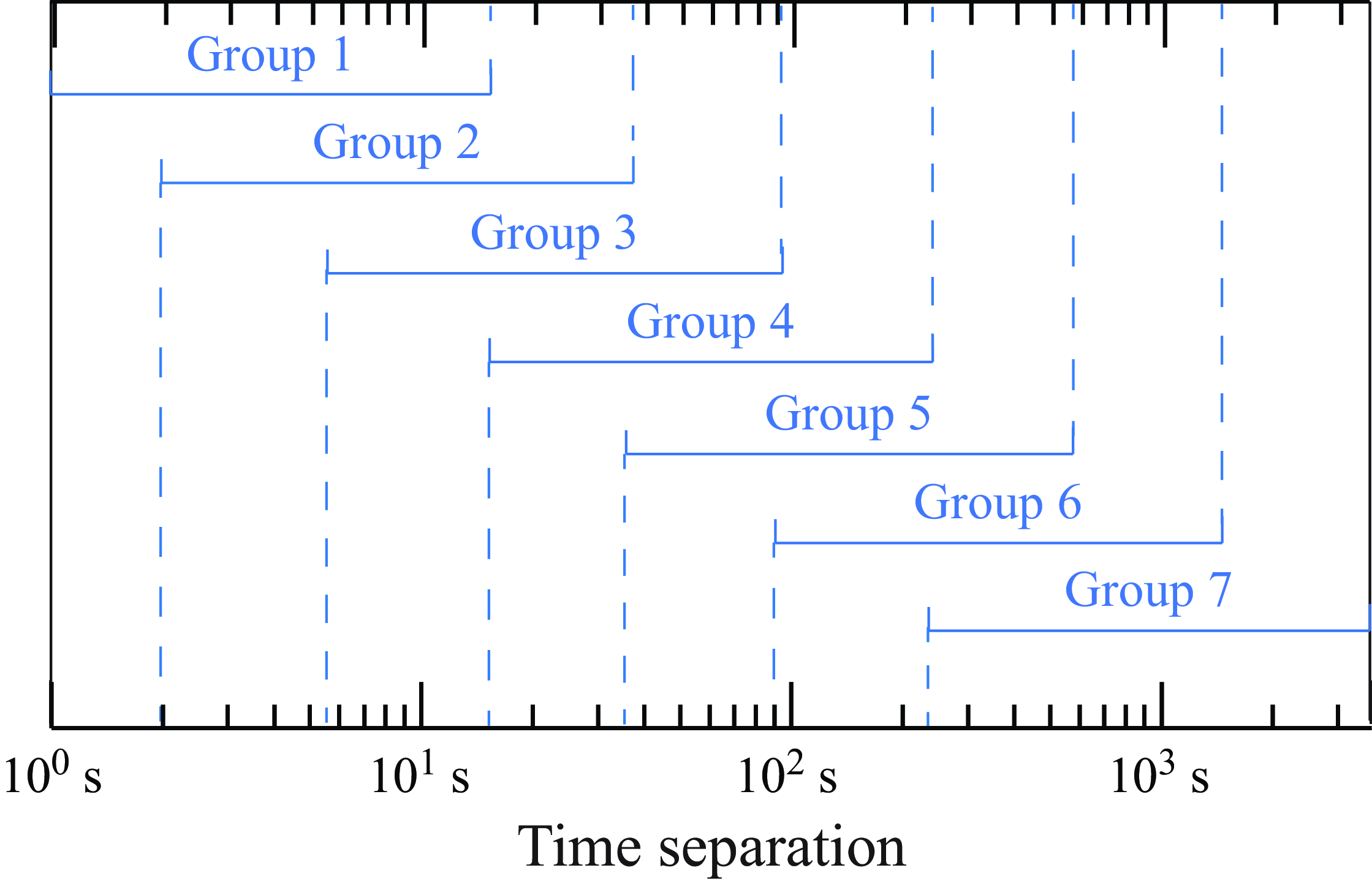
overlapping windows, each 1 h in duration. Time separations from 1 s to 1 h are considered in the analysis. In practice, it is challenging to identify a clear linear scaling over the entire range of time separations. To address this problem, as shown in figure 11, the whole time separations are divided into seven overlapping groups, each spanning over one decade. This ensures sufficient range for identifying potential linear scaling and facilitates the determination of the specific scales over which the magnetic helicity cascade becomes evident.
Time separation groups used to identify the linear scaling of the vKH relation.

Additionally, to recognise the cascade direction of the magnetic helicity, the magnetic helicity should be calculated. In the PSP data, only single-point measurement is available. When calculating the magnetic helicity, the difficulty is in evaluating the magnetic potential field
 $\boldsymbol a$
. Under the assumption of isotropy, Matthaeus & Goldstein (Reference Matthaeus and Goldstein1982) obtained the magnetic helicity (
 $H_M$
) spectrally. The same approach is adopted here to measure magnetic helicity. To examine its relationship with cross-helicity, we also evaluate the cross-helicity using this method. Accordingly, for each time series, the magnetic and cross-helicities are evaluated, respectively, as
 \begin{equation} \begin{aligned} &H_M= \left \langle \sum _{k}4\textrm{Im} \{\hat b_2 \hat b_3 \}/k \right \rangle _t ,\\ &H_C= \left \langle \sum _{k}{\textrm{Re}} \{\hat { \boldsymbol v}\boldsymbol{\cdot }\hat { \boldsymbol b}^\ast \} \right \rangle _t, \end{aligned} \end{equation}
where
 $\hat {\boldsymbol \cdot}$
represents the quantities in spectral space,
 $\textrm{Im}$
and
 ${\textrm{Re}}$
represent the imaginary and real parts of a complex value, respectively.
Two examples of magnetic helicity cascades on (a) 4 November 2018, 6:50–7:50 and (b) 8 November 2018, 21:11–22:11. Here,
 $\varepsilon _{\textit{HM}}$
denotes the estimated magnetic cascade rate.

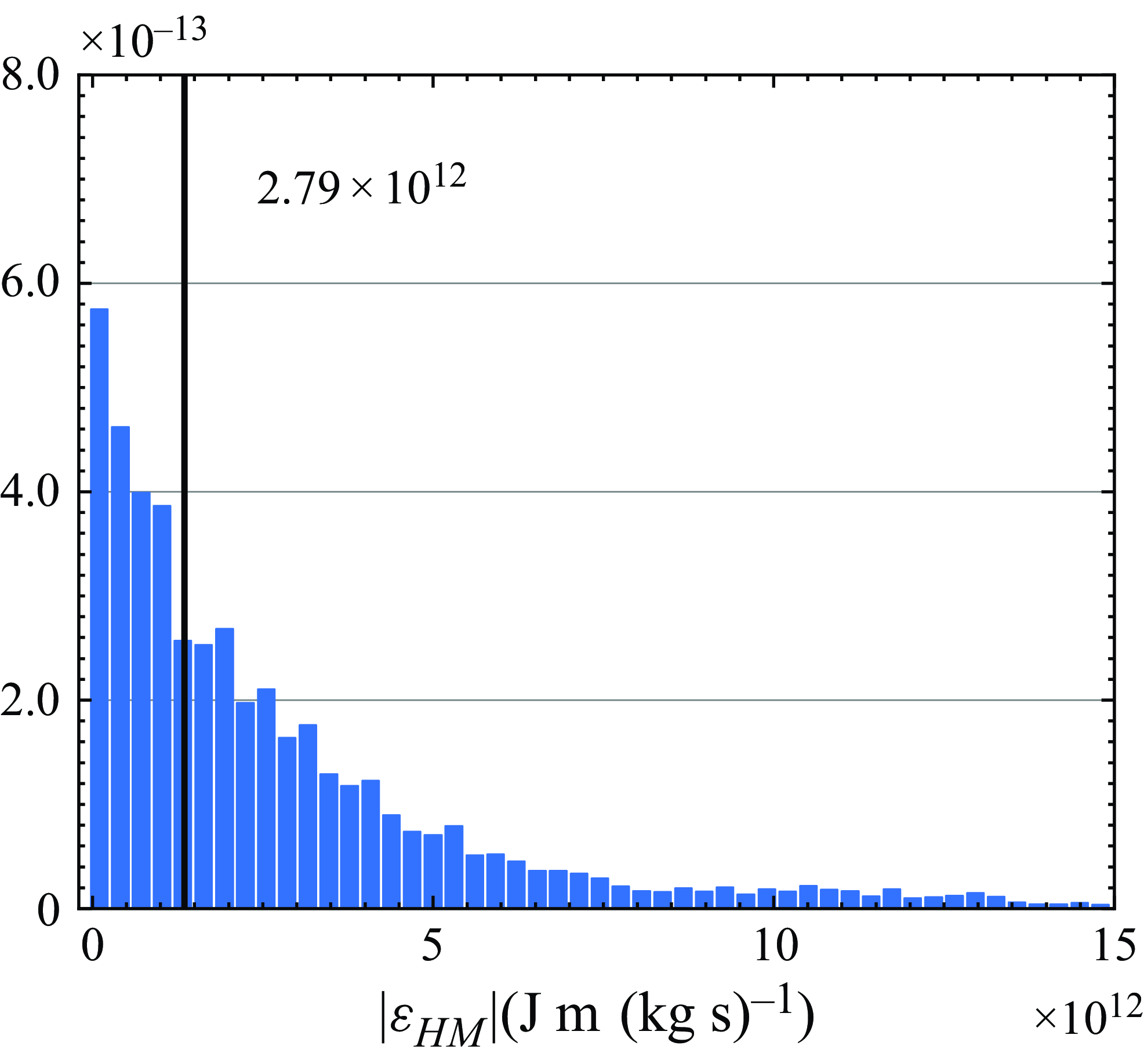
Probability distribution functions of the magnetic cascade rates. The black solid line shows the mean magnetic helicity cascade rate.

3.2. Data evaluation
With the newly derived vKH relation (3.1), the magnetic helicity cascade rates can be estimated as
 \begin{equation} \varepsilon _{\textit{HM}}={V_R\,\tau }/{[3V_{\textit{HM}}(\tau )]}. \end{equation}
Figure 12 presents two typical examples exhibiting the standard magnetic helicity cascades. As shown in figure 12 (b), on 8 November 2018, from 21:11 to 22:11,
 $V_{\textit{HM}}(\tau )$
is linear for nearly two decades with
 $\varepsilon _{\textit{HM}}=1.23\times 10^{13}\,{\textrm{J m (kg s)}}^{-1}$
. Figure 13 shows the PDF of
 $|\varepsilon _{\textit{HM}}|$
, with a mean value of
 $2.79\times 10^{12}\,{\textrm{J m (kg s)}}^{-1}$
.
Notably, the cross-helicity observed in the solar wind may also originate from mechanisms other than the Hall effect. Therefore, the numerical findings are assessed here in two aspects: the generation of cross-helicity and the suppression of cascade efficiency associated with it. Conditioned by the cascade direction, the relation between the cross-helicity (
 $H_C$
) and the magnetic helicity (
 $H_M$
) is shown in figure 14 (a). Regardless of the type of the cascade, strong cross-helicity is observed alongside a magnetic helicity cascade. Figure 14 (b) shows the cascade efficiency
 $\varGamma _{HMt}=|\varepsilon _{\textit{HM}}|/[|\delta {\boldsymbol v}||\delta {\boldsymbol b}|^2]$
versus the normalised cross-helicity
 $|h_{ct}|=|\delta {\boldsymbol v}\boldsymbol{\cdot }\delta {\boldsymbol b}|/|\delta {\boldsymbol v}||\delta {\boldsymbol b}|$
. Here,
 $|\delta {\boldsymbol v}\boldsymbol{\cdot }\delta {\boldsymbol b}|$
,
 $|\delta {\boldsymbol v}|$
and
 $|\delta {\boldsymbol b}|$
are averaged over the time separation group corresponding to magnetic helicity cascades (figure 11). As shown, the normalised cascade rate
 $\varGamma _{HMt}$
is suppressed by
 $|h_{ct}|$
, consistent with the numerical findings of this study.
Results from the solar wind data. (a) Relation between the cross-helicity
 $H_C$
and the magnetic helicity
 $H_M$
. Here,
 $\sigma$
represents the variance. (b) Cascade efficiency
 $\varGamma _{HMt}$
versus the normalised cross-helicity
 $|h_{ct}|$
.

4. Conclusions
In this paper, we use numerical simulations and solar wind data to investigate Hall effects on inverse cascades. We find that Hall effects could induce strong cross-helicity through geometric alignments between the velocity and magnetic fields. The cross-helicity then significantly reduces the inverse-cascade efficiencies and leads to the accumulation of magnetic energy and helicity at large scales. The process is associated with the disruption of current sheets due to the entrainment of sheets by vortex tubes or the excitation of whistler waves. Then, the numerical findings about the cross-helicity generation and the cascade efficiency suppression are separately confirmed by the solar wind observations from the PSP. In hydrodynamic turbulence, the turbulent strength on the inertial scale is solely determined by the cascade rates, and the Kolmogorov coefficient is universal for turbulent flows (Pope Reference Pope2000). However, the present results suggest that such universality may not hold in HMHD turbulence exhibiting inverse cascades. The turbulent intensity within the inverse-cascade range may be amplified by the presence of cross-helicity and Hall effects.
In the heliosphere, some extreme solar wind events originate from dynamic processes in the solar corona, where magnetic helicity and Hall effects play important roles. It is generally accepted that Hall effects can be assumed to be negligible at large scales in the solar wind (Marino & Sorriso-Valvo Reference Marino and Sorriso-Valvo2023), which justifies the use of MHD models at these scales. However, this study proposes a new mechanism in solar wind turbulence whereby Hall effects can significantly influence the large-scale magnetic field through cross-helicity. This mechanism may help explain how solar wind turbulence at larger scales can be strongly affected by processes occurring at the ion inertial scale, especially during extreme solar wind events with strongly helical magnetic fields.
Funding
This work was supported by the National Natural Science Foundation of China (Grants No. 12472229, No. 12072349, No. 12232018, No. 91852203, No. 12202457, No. 92052102 and No. 12272006) and the National Key Research and Development Program of China (Grant No. 2020YFA0711800).
Declaration of interests
The authors report no conflict of interest.
Appendix A. Derivation of two vKH relations for magnetic helicity
A.1. First vKH relation for the magnetic helicity
The governing equation for the magnetic potential
 $\boldsymbol a$
is
 \begin{equation} \begin{aligned} \partial _t {\boldsymbol a} & ={\boldsymbol U}\times {\boldsymbol b}+2\boldsymbol{\nabla }\psi +\lambda_b\Delta^{-1}\boldsymbol{b}-\eta (-\varDelta )^\alpha {\boldsymbol a}+{\boldsymbol f_{\!a}} , \\ \end{aligned} \end{equation}
where
 $2\boldsymbol{\nabla }\psi$
corresponds to an arbitrary choice of gauge, and
 $\boldsymbol{\nabla }\times \boldsymbol f_{\!a}=f_{b}$
.
For three arbitrary vectors
 $\boldsymbol p$
,
 $\boldsymbol q$
and
 $\boldsymbol o$
, the isotropic second- and third-order isotropic tensors without reflection symmetry (
 $R_{\textit{ij}}^{pq}= \langle p_i ({\boldsymbol x}) q_j({\boldsymbol x}') \rangle$
and
 $\varPhi _{ijl}^{opq}= \langle o_i({\boldsymbol x}) p_j ({\boldsymbol x}) q_l({\boldsymbol x})' \rangle$
) can be written as (Politano, Gomez & Pouquet Reference Politano, Gomez and Pouquet2003)
 \begin{equation} \begin{aligned} R_{\textit{ij}}^{pq}({\boldsymbol r})&=A^{pq}(r)r_i r_j+B^{pq}(r)\delta _{\textit{ij}}+\bar {C}^{pq}(r) \epsilon _{ijl}r_l,\\ \varPhi _{ijl}^{opq}({\boldsymbol r})&=a_{11}(r)r_l\delta _{\textit{ij}}+a_{12}(r)r_j\delta _{il}+a_{13}(r) r_i\delta _{jl}\\ &\quad +a_3(r)r_ir_jr_l +\bar b_{23}(r)r_i \epsilon _{jlm}r_m +\bar b_{22} (r)r_j\epsilon _{lim}r_m\\ &\quad +\bar b_{21}(r)r_l\epsilon _{ijm}r_m,\\ \end{aligned} \end{equation}
where
 $\boldsymbol r= \boldsymbol x'- \boldsymbol x$
is the displacement between two positions
 $\boldsymbol x$
and
 $\boldsymbol x'$
with a distance
 $r=|{\boldsymbol r}|$
,
 $\delta _{\textit{ij}}$
represents the Kronecker delta,
 $\epsilon _{ijl}$
is the Levi-Civita symbol,
 $A^{pq}(r), \,B^{pq}(r), \,\bar C^{pq}(r),\,a^{opq}_{11}(r), \,a^{opq}_{12}(r), \,a^{opq}_{12}(r), \,a^{opq}_{3}(r)$
,
 $\bar b^{opq}_{23}(r)$
,
 $\bar b^{opq}_{22}(r)$
and
 $ \,\bar b^{opq}_{21}(r)$
are functions of
 $r$
and
 $\,\bar {\boldsymbol \cdot}$
represents pseudoscalar.
According to (2.1) and (A1), the equation for the correlation function of magnetic helicity
 $R^{H_M}({\boldsymbol r})=R^{ab}_{ii}({\boldsymbol r})= \langle a_i ({\boldsymbol x}) b_i({\boldsymbol x}') \rangle$
can be written as
 \begin{equation} \partial _t R^{H_M}(r) = \langle {\boldsymbol b}'\boldsymbol{\cdot }{ \mathcal{ E}} \rangle +\left \langle {\boldsymbol a}\boldsymbol{\cdot }{\boldsymbol f_{\!b}}' \right \rangle -\eta\langle \boldsymbol{a} \boldsymbol{\cdot}(-\varDelta)^\alpha \boldsymbol{b}'\rangle +\lambda _{b}\big \langle {\boldsymbol a}\boldsymbol{\cdot }\varDelta ^{-1} {\boldsymbol b} '\big \rangle , \end{equation}
where
 ${ \mathcal{ E}}={\boldsymbol U} \times {\boldsymbol b}$
, and the superscript
 $'$
represents the quantities at
 $\boldsymbol x'$
. This equation is related to the homogeneous results given by Banerjee & Galtier (Reference Banerjee and Galtier2016b
). In the statistically steady state,
 $\partial _t R^{H_M}(r)=0$
. With the assumption of isotropy, the nonlinear terms can be written as
 \begin{equation} \begin{aligned} \langle {\boldsymbol b}'\boldsymbol{\cdot }\mathcal{E} \rangle &=R^{\mathcal{E}b}_{ii} =\frac {1}{r^2}\partial _r \big[r^3 R_{LL}^{\mathcal{E}b}\big]\\ &=\frac {1}{r^2}\partial _r \big[r^3 \big(\varPhi _{23L}^{Ubb}-\varPhi _{32L}^{Ubb}\big)\big],\\ \end{aligned} \end{equation}
where the subscript
 $L$
refers to the longitudinal direction (along
 $\boldsymbol r$
), and the subscripts 2 and 3 refer to the two remaining transverse directions. If the forcing and the dissipation terms are also isotropic, according to the results of Xie & Bühler (Reference Xie and Bühler2019), it can be further derived that
 \begin{equation} \frac {1}{r^2}\partial _r \big[r^3 \big(\varPhi _{23L}^{Ubb}-\varPhi _{32L}^{Ubb}\big)\big]= \int _0^\infty {\textrm{d}} K \frac {{\textrm{d}} F}{{\textrm{d}} K} \frac {\sin Kr}{Kr}, \end{equation}
where
 $F=-\varepsilon _{\textit{HMI}}+\sum _{k'\in \{k_f\}}{\varepsilon _M(k')} H(K-k')$
,
 $\varepsilon _{\textit{HMI}}$
is the inverse magnetic helicity flux,
 $\varepsilon_{M}(k')$
is the magnetic helicity injection at the forcing wavenumber and
 $H(K-k')$
is the Heaviside function. The integral of (A5) leads to
 \begin{equation} r\big(\varPhi _{23L}^{Ubb}({\boldsymbol r})-\varPhi _{32L}^{Ubb}({\boldsymbol r})\big) = \frac {1}{3}\varepsilon _{\textit{HMI}}\,r -\sum _{K=k_f}{\varepsilon _M}(K) \frac {\sin Kr-Kr\cos Kr}{K^3 r^2}. \end{equation}
The equation can also be written in structure function form as
 \begin{equation} \begin{aligned} V_{\textit{HM}1}&=\frac {r}{2}\langle \delta (U_3b_2-U_2b_3)\delta b_L\rangle \\ &=\frac {1}{3}\varepsilon _{\textit{HMI}}r-\sum _{K=k_f}{\varepsilon _M}(K) \frac {\sin Kr-Kr\cos Kr}{K^3 r^2},\\ \end{aligned} \end{equation}
where
 $\delta q_i=q_i({\boldsymbol x}')-q_i({\boldsymbol x})$
is the two-point increment for an arbitrary vector
 $\boldsymbol q$
.
A.2. Alternative formulation of the vKH relation for magnetic helicity
For a homogeneous quantity
 $ p ({\boldsymbol x})$
, there is a relation between
 $\partial _{\boldsymbol x}$
,
 $\partial _{\boldsymbol x'}$
and
 $\partial _{\boldsymbol r}$
 \begin{equation} -\partial _{x_i'} \left \langle p \right \rangle =\partial _{r_i} \left \langle p \right \rangle =\partial _{x_i}\left \langle p \right \rangle . \end{equation}
Utilising this relation (A8),
 $\varPhi _{lmj}^{vbb}({\boldsymbol r})$
can be written as
 \begin{equation} \begin{aligned} \varPhi _{lmj}^{vbb}({\boldsymbol r})= \epsilon _{jkn}\partial _{r_k}\varPhi _{lmn}^{vba}({\boldsymbol r}). \end{aligned} \end{equation}
The isotropic third-order structure function
 $\varPhi _{lmn}^{vba}({\boldsymbol r})= \langle v_l b_m a_n' \rangle$
is a pseudo-vector, and can be written as
 \begin{equation} \begin{aligned} \varPhi _{lmn}^{vba}({\boldsymbol r})&=\bar a_{11}^{vba}(r)r_n\delta _{lm}+\bar a_{12}^{vba}(r)r_m\delta _{ln}+\bar a_{13}^{vba}(r)r_l\delta _{mn}\\[4pt] &\quad +\bar a_3^{vba}(r)r_lr_mr_n + b_{23}^{vba}(r)r_l \varepsilon _{mnp}r_p + b_{22}^{vba} r_m\epsilon _{nlp}r_p\\[4pt] &\quad + b_{21}^{vba}(r)r_n\epsilon _{lmp}r_p.\\ \end{aligned} \end{equation}
According to the relation
 $\partial _{r_k}=({r_k}/{r})\partial _{r}$
, for the first three terms, the partial derivatives can be written as
 \begin{equation} \begin{aligned} \epsilon _{jkn}\partial _{r_k}&\big [\bar a_{11}^{vba}(r)r_n\delta _{lm}+\bar a_{12}^{vba}(r)r_m\delta _{ln}+\bar a_{13}^{vba}(r)r_l\delta _{mn}\big ]\\[3pt]=&\epsilon _{jkn}\left [ \big(\partial _r \bar a_{11}^{vba}\big) \frac {r_kr_n}{r} \delta _{lm} + \bar a_{11}^{vba} \delta _{kn} \delta _{lm}\right . \\[3pt]&\qquad +\left(\partial _r \bar a_{12}^{vba}\right) \frac {r_kr_m}{r}\delta _{ln} +\bar a_{12}^{vba} \delta _{km}\delta _{ln}\\[3pt]&\qquad \left . +\big(\partial _r \bar a_{13}^{vba}\big) \frac {r_kr_l}{r}\delta _{mn} +\bar a_{13}^{vba} \delta _{kl}\delta _{mn} \right ]\\[3pt]=&\epsilon _{jkl} \big(\partial _r \bar a_{12}^{vba}\big) \frac {r_kr_m}{r} +\epsilon _{jml} \bar a_{12}^{vba}\\[3pt]&\qquad +\epsilon _{jkm} \big(\partial _r \bar a_{13}^{vba}\big) \frac {r_kr_l}{r} +\epsilon _{jlm} \bar a_{13}^{vba}. \end{aligned} \end{equation}
If
 $\{l,m,j\}=\{2,3,L\}$
, then
 $r_l=r_m=0$
. In addition, there are two relations
 \begin{equation} \begin{aligned} \bar a_{13}^{vba}(r)r=\varPhi _{L22}^{vba}({\boldsymbol r})=\varPhi _{L33}^{vba}({\boldsymbol r}),\\ \bar a_{12}^{vba}(r)r=\varPhi _{2L2}^{vba}({\boldsymbol r})=\varPhi _{3L3}^{vba}({\boldsymbol r}).\\ \end{aligned} \end{equation}
Therefore, (A11) can be further simplified as
 \begin{equation} \begin{aligned} \epsilon _{jkn}\partial _{r_k}& \big [\bar a_{11}^{vba}(r)r_n\delta _{lm}+\bar a_{12}^{vba}(r)r_m\delta _{ln} +\bar a_{13}^{vba}(r)r_l\delta _{mn}\big ] \big |_{\{l,m,j\}=\{2,3,L\}}\\[3pt] &=\bar a_{13}^{vba}(r)-\bar a_{12}^{vba}(r) =\varPhi _{L22}^{vba}({\boldsymbol r})-\varPhi _{2L2}^{vba}({\boldsymbol r}). \end{aligned} \end{equation}
By similar derivation, the curls of the other four terms in (A10) are zero
 \begin{equation} \begin{aligned} \epsilon _{jkn}\partial _{r_k}& \big[\bar a_3^{vba}(r)r_lr_mr_n + b_{23}^{vba}(r)r_l \varepsilon _{mnp}r_p + b_{22}^{vba} r_m\epsilon _{nlp}r_p \\[3pt] & + b_{21}^{vba}(r)r_n\epsilon _{lmp}r_p \big]\big|_{\{l,m,j\}=\{2,3,L\}}=0. \end{aligned} \end{equation}
Therefore, it can be obtained from (A9), (A10), (A13) and (A14) that
 \begin{equation} \varPhi _{23L}^{vbb}({\boldsymbol r}) = \big(\varPhi _{L22}^{vba}({\boldsymbol r})-\varPhi _{2L2}^{vba}({\boldsymbol r})\big)/r. \end{equation}
It can be derived from (A2) that
 \begin{equation} \varPhi _{23L}^{vbb}({\boldsymbol r})=-\varPhi _{32L}^{vbb}({\boldsymbol r})=r^2 \bar b_{21}(r). \end{equation}
Therefore, (A15) can be rewritten as
 \begin{equation} r\big(\varPhi _{23L}^{vbb}({\boldsymbol r})-\varPhi _{32L}^{vbb}({\boldsymbol r})\big)=2\big(\varPhi _{L22}^{vba}({\boldsymbol r})-\varPhi _{2L2}^{vba}({\boldsymbol r})\big). \end{equation}
Now, we concentrate on the alternative form of the Hall effects:
 $-d_Ir(\varPhi _{23L}^{jbb}({\boldsymbol r})-\varPhi _{32L}^{jbb}({\boldsymbol r}))$
.
Using
 $\boldsymbol (\boldsymbol{\nabla }\times \boldsymbol{b}) \times \boldsymbol{b}= (\boldsymbol{b} \boldsymbol{\cdot }\boldsymbol{\nabla }) \boldsymbol{b} -\boldsymbol{\nabla }|\boldsymbol{b}|^{\textrm{2}}/\textrm{2}$
and (A8), there are following relations:
 \begin{equation} \begin{aligned} \varPhi _{23L}^{jbb}({\boldsymbol r})-\varPhi _{32L}^{jbb}({\boldsymbol r}) =-\partial _{r_i}\varPhi ^{bbb}_{LiL}({\boldsymbol r})+\frac {1}{2}\partial _{r_L}\varPhi ^{bbb}_{iiL}({\boldsymbol r}). \end{aligned} \end{equation}
According to (A2),
 $\varPhi _{LiL}^{bbb}({\boldsymbol r})$
can be written as
 \begin{equation} \varPhi _{LiL}^{bbb}({\boldsymbol r}) = {\bar a}_{11}^{bbb}(r)r_L\delta _{Li}+ {\bar a}_{12}^{bbb}(r)r_i+ {\bar a}_{13}^{bbb}(r)r_L\delta _{iL} + {\bar a}_3(r)^{bbb}r^2r_i. \end{equation}
Then,
 $\partial _{r_i}\varPhi ^{bbb}_{LiL}({\boldsymbol r})$
in (A18) can be written as
 \begin{equation} \begin{aligned} \partial _{r_i}\varPhi ^{bbb}_{LiL}({\boldsymbol r})&= r\partial _r {\bar a}_{11}^{bbb}(r)+ {\bar a}_{11}^{bbb}(r) +r\partial _r {\bar a}_{12}^{bbb}(r)\\[3pt] &\quad + 3{\bar a}_{12}^{bbb}(r) +r\partial _r {\bar a}_{13}^{bbb}(r)+ {\bar a}_{13}^{bbb}(r)\\[3pt] &\quad +r^3\partial _r {\bar a}_{3}^{bbb}(r)+ 5r^2{\bar a}_{3}^{bbb}(r). \end{aligned} \end{equation}
For incompressible flow, there are the following relations for isotropic third-order structure functions (Politano et al. Reference Politano, Gomez and Pouquet2003):
 \begin{equation} \left \{ \begin{aligned} &r\partial _r{\bar a}_{11}^{bbb}(r)+3{\bar a}_{11}^{bbb}(r)+{\bar a}_{12}^{bbb}(r)+{\bar a}_{13}^{bbb}(r)=0, \\[3pt]&\frac {1}{r}\big(\partial _r{\bar a}_{12}^{bbb}(r)+\partial _r{\bar a}_{13}^{bbb}(r)\big)+r\partial _r{\bar a}_{3}^{bbb}(r)+5{\bar a}_{3}^{bbb}(r)=0,\\[3pt]&3{\bar a}_{11}^{bbb}(r)+{\bar a}_{12}^{bbb}(r)+{\bar a}_{13}^{bbb}(r)+r^2{\bar a}_{3}^{bbb}(r)=0.\\ \end{aligned} \right . \end{equation}
Using these relations, (A20) can be simplified as
 \begin{equation} \begin{aligned} \partial _{r_i}\varPhi ^{bbb}_{LiL}({\boldsymbol r})&= \frac {1}{r}\varPhi _{Lii}^{bbb}({\boldsymbol r}). \end{aligned} \end{equation}
According to the incompressible relation (A21),
 $\partial _{r_L}\varPhi _{iiL}^{bbb}({\boldsymbol r})$
in (A18) can be derived as
 \begin{equation} \partial _{r_L}\varPhi _{iiL}^{bbb}({\boldsymbol r}) = \partial _{r_L}\big \{\big[3{\bar a}_{11}^{bbb}(r)+ {\bar a}_{12}^{bbb}(r)+ {\bar a}_{13}^{bbb}(r) + {\bar a}_3^{bbb}(r)r^2 \big]r_L \big \}=0. \end{equation}
Then, according to (A18), (A22), and (A23), the Hall effects can be rewritten as
 \begin{equation} \begin{aligned} -d_Ir\big(\varPhi _{23L}^{jbb}({\boldsymbol r})-\varPhi _{32L}^{jbb}({\boldsymbol r})\big) =d_I\varPhi _{Lii}^{bbb}({\boldsymbol r}). \end{aligned} \end{equation}
According to (A17) and (A24), the alternative formulation for vKH relations can be written as
 \begin{equation} {r}\big(\varPhi _{23L}^{Ubb}({\boldsymbol r}) -\varPhi _{32L}^{Ubb}({\boldsymbol r})\big) =2\big[\varPhi _{L22}^{vba}({\boldsymbol r})-\varPhi _{2L2}^{vba}({\boldsymbol r})\big]+{d_I}\varPhi ^{bbb}_{Lii}({\boldsymbol r}). \end{equation}
The above vKH relations can be written in two-point increments and averages. For example,
 $\varPhi _{L22}^{vba}({\boldsymbol r})$
can be replaced by
 $- \langle \delta (v_Lb_2) a_2^\ast \rangle$
 \begin{equation} \begin{aligned} \left \langle \delta (v_Lb_2) a_2^\ast \right \rangle &=\left \langle v_L({\boldsymbol x}')b_2({\boldsymbol x}')a_2({\boldsymbol x})-v_L({\boldsymbol x})b_2({\boldsymbol x})a_2({\boldsymbol x}') \right \rangle /2\\[3pt] &=\left \langle v_L({\boldsymbol x})b_2({\boldsymbol x})a_2({\boldsymbol x-\boldsymbol{r}})- v_L({\boldsymbol x})b_2({\boldsymbol x})a_2({\boldsymbol x}') \right \rangle /2\\[3pt] &=\big[\varPhi _{L22}^{vba}(-{\boldsymbol r})-\varPhi _{L22}^{vba}({\boldsymbol r})\big]/2 =-r{\bar a}_{13}^{vba}(r)\\[3pt] &=-\varPhi _{L22}^{vba}({\boldsymbol r}), \end{aligned} \end{equation}
where
 $q_i^\ast ({\boldsymbol r})=[q_i({\boldsymbol x})+q_i({\boldsymbol x}')]/2$
for an arbitrary vector
 $\boldsymbol q$
. Using two-point increments and averages, the right-hand side of (A25) can be written as
 \begin{equation} \begin{aligned} V_{\textit{HM}2}=2\left \langle \delta (v_2b_L-v_Lb_2) a_2^\ast \right \rangle -{d_I}\left \langle \delta (b_Lb_i) b_i^\ast \right \rangle\! . \end{aligned} \end{equation}
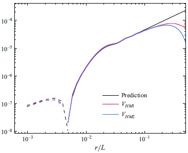
Numerical verifications of
 $V_{\textit{HM}1}$
and
 $V_{\textit{HM}2}$
using H40. Solid lines: positive values; dashed lines: negative values.

In conclusion, (A7) and (A27) give two estimations for magnetic helicity cascade rates. Figure 15 verifies the two vKH relations using the results of H40, where black curves are predictions in (A7), with
 $\varepsilon _{\textit{HMI}}=4.4\times 10^{-4}$
and
 $\varepsilon_{M}=5.4\times 10^{-4}/3$
.
Considering that the potential
 $\boldsymbol a$
and current density
 $\boldsymbol j$
are hard to be obtained in solar wind observation,
 $V_{\textit{HM}1}$
and
 $V_{\textit{HM}2}$
can be combined as
 \begin{equation} V_{\textit{HM}} =\frac {r}{2}\left \langle \delta (v_3b_2-v_2b_3)\delta b_L \right \rangle -{d_I}\left \langle \delta (b_Lb_i) b_i^\ast \right \rangle\! , \end{equation}
where
 $\delta q_i=q_i({\boldsymbol x}')-q_i({\boldsymbol x})$
is the two-point increment for an arbitrary vector
 $\boldsymbol q$
.