2.1 Model equations

Calling on Sammarco et al. (Reference Sammarco, Cecioni, Bellotti and Abdolali2013), consider the motion of a slightly compressible fluid of density $\unicode[STIX]{x1D70C}=\unicode[STIX]{x1D70C}_{0}+\unicode[STIX]{x1D70C}^{\prime }$ , where $\unicode[STIX]{x1D70C}_{0}$ is the constant ambient density and $\unicode[STIX]{x1D70C}^{\prime }\ll \unicode[STIX]{x1D70C}_{0}$ is a small perturbation due to compressibility. Let $(\boldsymbol{x},z)=(x,y,z)$ describe the coordinate of a point in a 3-D fluid domain ${\mathcal{D}}$ , with the $z$ axis orthogonal to the horizontal $(x,y)$ plane and pointing upwards from the unperturbed water level $z=0$ . The bottom of the ocean is at $z=-h(\boldsymbol{x})+H(\boldsymbol{x},t)$ , where $h(\boldsymbol{x})$ is a fixed impermeable surface and $H(\boldsymbol{x},t)$ a prescribed time-dependent seafloor motion; $t$ denotes time. The boundary-value problem for a weakly compressible, inviscid fluid and irrotational motion is:

(2.1) $$\begin{eqnarray}\displaystyle & \displaystyle \unicode[STIX]{x1D6F7}_{tt}=c^{2}(\unicode[STIX]{x1D6FB}^{2}\unicode[STIX]{x1D6F7}+\unicode[STIX]{x1D6F7}_{zz}),\quad (\boldsymbol{x},z)\in {\mathcal{D}}, & \displaystyle\end{eqnarray}$$

(2.2) $$\begin{eqnarray}\displaystyle & \displaystyle \unicode[STIX]{x1D6F7}_{tt}+g\unicode[STIX]{x1D6F7}_{z}=0,\quad z=0, & \displaystyle\end{eqnarray}$$

(2.3) $$\begin{eqnarray}\displaystyle & \displaystyle \unicode[STIX]{x1D6F7}_{z}+\unicode[STIX]{x1D735}h\boldsymbol{\cdot }\unicode[STIX]{x1D735}\unicode[STIX]{x1D6F7}=-H_{t},\quad z=-h(\boldsymbol{x}). & \displaystyle\end{eqnarray}$$

In the latter system of equations, $\unicode[STIX]{x1D6F7}(\boldsymbol{x},z,t)$ is the 3-D velocity potential, $g$ is the acceleration due to gravity and $c=1480~\text{m}~\text{s}^{-1}$ is the speed of sound in water, assumed constant. Also, $\unicode[STIX]{x1D735}f(\boldsymbol{x})=(f_{x},f_{y})$ is the 2-D gradient and subscripts denote differentiation with respect to the relevant variable. The system (2.1)–(2.3) describes acoustic–gravity waves generated by the bottom disturbance $H$ and is the same as that considered by Sammarco et al. (Reference Sammarco, Cecioni, Bellotti and Abdolali2013). In this paper we shall develop a mathematical method to solve the system of governing equations (2.1)–(2.3) analytically. First, we shall adopt a Galerkin approach (Massel Reference Massel2013) to derive the governing partial differential equation (PDE) in the horizontal plane. Then we shall solve it by combining a multiple-scale perturbation approach with asymptotic analysis. We formulate the mathematical problem for a generic single frequency $f$ of the forcing spectrum, assuming the decompositions:

(2.4a,b ) $$\begin{eqnarray}H(\boldsymbol{x},t)=\text{Re}\,\{\bar{H}(\boldsymbol{x})\,\text{e}^{-\text{i}\unicode[STIX]{x1D714}t}\},\quad \unicode[STIX]{x1D6F7}(\boldsymbol{x},z,t)=\text{Re}\,\{\bar{\unicode[STIX]{x1D6F7}}(\boldsymbol{x},z)\text{e}^{-\text{i}\unicode[STIX]{x1D714}t}\},\end{eqnarray}$$

where $\text{i}$ is the imaginary unit and $\unicode[STIX]{x1D714}=2\unicode[STIX]{x03C0}f$ is the angular frequency. $\text{Re}\,\{\cdot \}$ denotes the real part and will be omitted in the following for the sake of brevity. Results for generic time-dependent disturbances can be found by Fourier superposition of the harmonic solution $\unicode[STIX]{x1D6F7}$ (Mei, Stiassnie & Yue Reference Mei, Stiassnie and Yue2005; Sammarco et al. Reference Sammarco, Cecioni, Bellotti and Abdolali2013). Using (2.4), the system (2.1)–(2.3) becomes

(2.5) $$\begin{eqnarray}\displaystyle & \displaystyle \left(\unicode[STIX]{x1D6FB}^{2}+\frac{\unicode[STIX]{x1D714}^{2}}{c^{2}}\right)\bar{\unicode[STIX]{x1D6F7}}+\bar{\unicode[STIX]{x1D6F7}}_{zz}=0,\quad (\boldsymbol{x},z)\in {\mathcal{D}}, & \displaystyle\end{eqnarray}$$

(2.6) $$\begin{eqnarray}\displaystyle & \displaystyle \bar{\unicode[STIX]{x1D6F7}}_{z}-\frac{\unicode[STIX]{x1D714}^{2}}{g}\bar{\unicode[STIX]{x1D6F7}}=0,\quad z=0, & \displaystyle\end{eqnarray}$$

(2.7) $$\begin{eqnarray}\displaystyle & \displaystyle \bar{\unicode[STIX]{x1D6F7}}_{z}+\unicode[STIX]{x1D735}h\boldsymbol{\cdot }\unicode[STIX]{x1D735}\bar{\unicode[STIX]{x1D6F7}}=\text{i}\unicode[STIX]{x1D714}\bar{H},\quad z=-h(\boldsymbol{x}), & \displaystyle\end{eqnarray}$$

where the complex potential $\bar{\unicode[STIX]{x1D6F7}}(\boldsymbol{x},z)$ must be bounded in the fluid domain ${\mathcal{D}}$ . Now expand the spatial potential into a Galerkin series (Massel Reference Massel2013)

(2.8) $$\begin{eqnarray}\bar{\unicode[STIX]{x1D6F7}}(\boldsymbol{x},z)=\mathop{\sum }_{n=0}^{\infty }\bar{\unicode[STIX]{x1D6F7}}_{n}(\boldsymbol{x},z)=\mathop{\sum }_{n=0}^{\infty }\unicode[STIX]{x1D719}_{n}(\boldsymbol{x})Z_{n}(\boldsymbol{x},z),\end{eqnarray}$$

where

(2.9) $$\begin{eqnarray}Z_{n}(\boldsymbol{x},z)=\frac{\sqrt{2}\cosh [\unicode[STIX]{x1D6FD}_{n}(z+h)]}{\left[h+\displaystyle \frac{g}{\unicode[STIX]{x1D714}^{2}}\sinh ^{2}(\unicode[STIX]{x1D6FD}_{n}h)\right]^{1/2}}.\end{eqnarray}$$

In (2.9) the $\unicode[STIX]{x1D6FD}_{n}=\unicode[STIX]{x1D6FD}_{n}[h(\boldsymbol{x})]$ are the solutions of the dispersion relation:

(2.10) $$\begin{eqnarray}\displaystyle \unicode[STIX]{x1D714}^{2}=g\unicode[STIX]{x1D6FD}_{0}\tanh \,(\unicode[STIX]{x1D6FD}_{0}h),\quad n=0, & & \displaystyle\end{eqnarray}$$

(2.11a,b ) $$\begin{eqnarray}\displaystyle \unicode[STIX]{x1D6FD}_{n}=\text{i}\tilde{\unicode[STIX]{x1D6FD}}_{n},\quad \unicode[STIX]{x1D714}^{2}=-g\tilde{\unicode[STIX]{x1D6FD}}_{n}\tan (\tilde{\unicode[STIX]{x1D6FD}}_{n}h),\quad n>0. & & \displaystyle\end{eqnarray}$$

The 0th mode represents the surface gravity wave, which is hardly influenced by compressibility (Yamamoto Reference Yamamoto1982; Stiassnie Reference Stiassnie2010; Renzi & Dias Reference Renzi and Dias2014a ). The higher modes $n>0$ represent the associated HA waves, which for given frequency $\unicode[STIX]{x1D714}$ can be either evanescent or propagating at large $|\boldsymbol{x}|$ , depending on the system parameters (see § 3). Now introduce the inner product

(2.12) $$\begin{eqnarray}\langle f(z),g(z)\rangle =\int _{-h(\boldsymbol{x})}^{0}f(z)g(z)\,\text{d}z,\end{eqnarray}$$

which together with (2.10)–(2.11a,b ) yields $\langle Z_{n},Z_{m}\rangle =\unicode[STIX]{x1D6FF}_{nm}$ . Hence the $Z_{n}$ are a set of orthonormal eigenfunctions in $(-h(\boldsymbol{x}),0)$ . The eigenfunctions (2.9) are a normalised form of those used in the solution of Sammarco et al. (Reference Sammarco, Cecioni, Bellotti and Abdolali2013), namely $f_{n}=\cosh \,[\unicode[STIX]{x1D6FD}_{n}(z+h)]/\cosh \,(\unicode[STIX]{x1D6FD}_{n}h)$ . Note that the latter expression becomes singular for $z<0$ in the limit $\unicode[STIX]{x1D6FD}_{n}\rightarrow \text{i}(2n-1)\unicode[STIX]{x03C0}/(2h)$ , which describes the HA modes of the system (Yamamoto Reference Yamamoto1982; Stiassnie Reference Stiassnie2010). Such a singularity would prevent us from obtaining an analytical representation of the HA field quantities (though a numerical solution is still possible, see Sammarco et al. Reference Sammarco, Cecioni, Bellotti and Abdolali2013). Conversely, the normalised eigenfunctions (2.9) allow us to solve the problem analytically. Now, let us expand $\bar{H}$ into a Galerkin series too

(2.13) $$\begin{eqnarray}\displaystyle \bar{H}(\boldsymbol{x})=\mathop{\sum }_{n=0}^{\infty }\bar{H}_{n}(\boldsymbol{x})=\mathop{\sum }_{n=0}^{\infty }H_{n}(\boldsymbol{x})Z_{n}(\boldsymbol{x},z), & & \displaystyle\end{eqnarray}$$

where the expansion terms

(2.14) $$\begin{eqnarray}\displaystyle H_{n}(\boldsymbol{x})=\bar{H}(\boldsymbol{x})\,\frac{2\sinh (\unicode[STIX]{x1D6FD}_{n}h)}{[2\unicode[STIX]{x1D6FD}_{n}^{2}h+\unicode[STIX]{x1D6FD}_{n}\sinh (2\unicode[STIX]{x1D6FD}_{n}h)]^{1/2}} & & \displaystyle\end{eqnarray}$$

follow from the orthogonality of the $Z_{n}$  (2.9). We are now in a position to derive a depth-averaged form for the boundary-value problem (2.5)–(2.7). By following the depth-averaged approach of Sammarco et al. (Reference Sammarco, Cecioni, Bellotti and Abdolali2013), but using the orthonormal eigenfunctions (2.9), we get a normalised version of the mild-slope equation for weakly compressible fluids (MSEWC):

(2.15) $$\begin{eqnarray}\unicode[STIX]{x1D6FB}^{2}\unicode[STIX]{x1D719}_{n}+\left(\frac{\unicode[STIX]{x1D714}^{2}}{c^{2}}+\unicode[STIX]{x1D6FD}_{n}^{2}\right)\unicode[STIX]{x1D719}_{n}=\text{i}\unicode[STIX]{x1D714}\unicode[STIX]{x1D6FE}_{n}H_{n},\quad n=0,1,\ldots ,\end{eqnarray}$$

where

(2.16) $$\begin{eqnarray}\unicode[STIX]{x1D6FE}_{n}(\boldsymbol{x})=\frac{4\unicode[STIX]{x1D6FD}_{n}}{2\unicode[STIX]{x1D6FD}_{n}h+\sinh (2\unicode[STIX]{x1D6FD}_{n}h)}\end{eqnarray}$$

has the dimension of a wavenumber. The 0th mode of (2.15) represents a progressive acoustic–gravity wave (Sammarco et al. Reference Sammarco, Cecioni, Bellotti and Abdolali2013). Due to the large difference between gravity and HA wave propagation speed in water, the gravity mode $n=0$ is hardly influenced by compressibility (Stiassnie Reference Stiassnie2010). Numerous analytical and numerical models for the gravity mode propagation over a slowly varying bottom are already available in the literature (e.g. Mei et al. Reference Mei, Stiassnie and Yue2005; Massel Reference Massel2013) and will not be discussed further. Here we shall focus on the HA modes $n\geqslant 1$ of (2.15).

2.2 The mild-slope equation (MSE) for HA waves

As anticipated in § 2.1, a good approximation for the HA wavenumbers $\unicode[STIX]{x1D6FD}_{n}=\text{i}\tilde{\unicode[STIX]{x1D6FD}}_{n}$ is

(2.17) $$\begin{eqnarray}\tilde{\unicode[STIX]{x1D6FD}}_{n}[h(\boldsymbol{x})]=\frac{(2n-1)\unicode[STIX]{x03C0}}{2h(\boldsymbol{x})},\end{eqnarray}$$

see for example Yamamoto (Reference Yamamoto1982), Stiassnie (Reference Stiassnie2010) and Renzi & Dias (Reference Renzi and Dias2014a ). As a consequence, the eigenmodes (2.9) become

(2.18) $$\begin{eqnarray}Z_{n}(\boldsymbol{x},z)=\sqrt{\frac{2}{h(\boldsymbol{x})}}\cos \left[(2n-1)\frac{\unicode[STIX]{x03C0}}{2}\left(1+\frac{z}{h(\boldsymbol{x})}\right)\right],\end{eqnarray}$$

the forcing terms (2.14) become

(2.19) $$\begin{eqnarray}H_{n}(\boldsymbol{x})=\frac{(-1)^{n+1}}{(n-\frac{1}{2})\unicode[STIX]{x03C0}}\sqrt{2h(\boldsymbol{x})}\,\bar{H}(\boldsymbol{x})\end{eqnarray}$$

and (2.16) simplifies to $\unicode[STIX]{x1D6FE}_{n}(\boldsymbol{x})=2/h(\boldsymbol{x})$ . Substituting the latter expressions into (2.15), one obtains the sought equation for the HA modes:

(2.20) $$\begin{eqnarray}\unicode[STIX]{x1D6FB}^{2}\unicode[STIX]{x1D719}_{n}+k_{n}^{2}(\boldsymbol{x})\,\unicode[STIX]{x1D719}_{n}=-\frac{4}{\unicode[STIX]{x03C0}}\frac{(-1)^{n}}{2n-1}\text{i}\unicode[STIX]{x1D714}\bar{H}(\boldsymbol{x})\sqrt{\frac{2}{h(\boldsymbol{x})}},\quad n=1,2,\ldots ,\end{eqnarray}$$

where

(2.21) $$\begin{eqnarray}k_{n}(\boldsymbol{x})=\sqrt{\frac{\unicode[STIX]{x1D714}^{2}}{c^{2}}-\frac{(2n-1)^{2}\unicode[STIX]{x03C0}^{2}}{4h^{2}(\boldsymbol{x})}}\end{eqnarray}$$

is the horizontal index of refraction of the $n$ th HA mode. Expression (2.20) is a specific form of the normalised MSEWC. We name (2.20) the MSE for HA waves (MSEHA).

3.1 General solution

In this section we study the homogeneous form of the MSEHA (2.20), which describes free incoming and outgoing HA waves, in the absence of tsunamigenic forcing. From now on we consider a generic HA mode, say $n\in \mathbb{N}$ , on a slowly varying topography in the two horizontal dimensions (2HD), $h=h(\unicode[STIX]{x1D716}\boldsymbol{x})$ , $\unicode[STIX]{x1D716}\ll 1$ . We shall now derive a multiple-scale approximation of the spatial HA potential $\unicode[STIX]{x1D719}_{n}(\boldsymbol{x})$ . Introduction of the slow variables

(3.1a,b ) $$\begin{eqnarray}\unicode[STIX]{x1D709}=\unicode[STIX]{x1D716}x,\quad \unicode[STIX]{x1D702}=\unicode[STIX]{x1D716}y,\end{eqnarray}$$

transforms the homogeneous version of (2.20) into

(3.2) $$\begin{eqnarray}\unicode[STIX]{x1D716}^{2}\tilde{\unicode[STIX]{x1D6FB}}^{2}\unicode[STIX]{x1D719}_{n}+k_{n}^{2}(\unicode[STIX]{x1D709},\unicode[STIX]{x1D702})\unicode[STIX]{x1D719}_{n}=0,\end{eqnarray}$$

where $\tilde{\unicode[STIX]{x1D735}}=(\unicode[STIX]{x2202}/\unicode[STIX]{x2202}\unicode[STIX]{x1D709},\unicode[STIX]{x2202}/\unicode[STIX]{x2202}\unicode[STIX]{x1D702})$ is the nabla operator in the slow coordinates. We will first consider the case of real $k_{n}$ and deal with complex wavenumbers later on. Note that, in the much simpler 1-D case over a flat bottom, where $k_{n}=\text{const.}$ , the spatial potential would be a combination of $\unicode[STIX]{x1D719}_{n}(\unicode[STIX]{x1D709})=\exp (\pm \text{i}k_{n}\unicode[STIX]{x1D709}/\unicode[STIX]{x1D716})$ , see e.g. Jensen et al. (Reference Jensen, Kuperman, Porter and Schmidt2011). For a 2HD varying bathymetry, by similarity we look for solutions of the form

(3.3) $$\begin{eqnarray}\unicode[STIX]{x1D719}_{n}(\unicode[STIX]{x1D709},\unicode[STIX]{x1D702})=A_{n}(\unicode[STIX]{x1D709},\unicode[STIX]{x1D702})\exp \left[\frac{\text{i}}{\unicode[STIX]{x1D716}}S_{n}(\unicode[STIX]{x1D709},\unicode[STIX]{x1D702})\right],\end{eqnarray}$$

where $A_{n}(\unicode[STIX]{x1D709},\unicode[STIX]{x1D702})$ and $S_{n}(\unicode[STIX]{x1D709},\unicode[STIX]{x1D702})$ are unknown real amplitude and phase functions, respectively. Equation (3.3) is a multiple-scale Wentzel–Kramers–Brillouin (WKB) expression, in which the wave amplitude varies with the slow coordinates $\unicode[STIX]{x1D709}$ and $\unicode[STIX]{x1D702}$ , while the phase varies with the fast coordinates $(\unicode[STIX]{x1D709},\unicode[STIX]{x1D702})\unicode[STIX]{x1D716}^{-1}$ , see Bender & Orszag (Reference Bender and Orszag1999). Substituting (3.3) into (3.2) and taking the real and imaginary parts of (3.2) separately zero, we get a system of two nonlinear PDEs:

(3.4) $$\begin{eqnarray}\unicode[STIX]{x1D716}^{2}\tilde{\unicode[STIX]{x1D6FB}}^{2}A_{n}-|\tilde{\unicode[STIX]{x1D735}}S_{n}|^{2}A_{n}+k_{n}^{2}A_{n}=0,\end{eqnarray}$$

(3.5) $$\begin{eqnarray}2\tilde{\unicode[STIX]{x1D735}}A_{n}\boldsymbol{\cdot }\tilde{\unicode[STIX]{x1D735}}S_{n}+A_{n}\tilde{\unicode[STIX]{x1D6FB}}^{2}S_{n}=0.\end{eqnarray}$$

Note that the original equation (3.2) and the system (3.4) and (3.5) are absolutely equivalent, for only the substitution (3.3) has been made so far. Let us now expand the amplitude and phase functions, respectively

(3.6) $$\begin{eqnarray}A_{n}(\unicode[STIX]{x1D709},\unicode[STIX]{x1D702})=A_{n}^{(0)}(\unicode[STIX]{x1D709},\unicode[STIX]{x1D702})+\unicode[STIX]{x1D716}A_{n}^{(1)}(\unicode[STIX]{x1D709},\unicode[STIX]{x1D702})+O(\unicode[STIX]{x1D716}^{2})\end{eqnarray}$$

and

(3.7) $$\begin{eqnarray}S_{n}(\unicode[STIX]{x1D709},\unicode[STIX]{x1D702})=S_{n}^{(0)}(\unicode[STIX]{x1D709},\unicode[STIX]{x1D702})+\unicode[STIX]{x1D716}S_{n}^{(1)}(\unicode[STIX]{x1D709},\unicode[STIX]{x1D702})+O(\unicode[STIX]{x1D716}^{2}),\end{eqnarray}$$

where $\unicode[STIX]{x1D716}\ll 1$ . Substitution of (3.6) and (3.7) into the system (3.4) and (3.5) yields, respectively, an eikonal equation

(3.8) $$\begin{eqnarray}|\tilde{\unicode[STIX]{x1D735}}S_{n}^{(0)}(\unicode[STIX]{x1D709},\unicode[STIX]{x1D702})|^{2}=k_{n}^{2}(\unicode[STIX]{x1D709},\unicode[STIX]{x1D702}),\end{eqnarray}$$

and a transport equation

(3.9) $$\begin{eqnarray}\tilde{\unicode[STIX]{x1D735}}\boldsymbol{\cdot }\{[A_{n}^{(0)}(\unicode[STIX]{x1D709},\unicode[STIX]{x1D702})]^{2}\tilde{\unicode[STIX]{x1D735}}S_{n}^{(0)}(\unicode[STIX]{x1D709},\unicode[STIX]{x1D702})\}=0,\end{eqnarray}$$

of the order $O(1)$ . The eikonal equation (3.8) can be solved numerically to obtain $S_{n}^{(0)}$ for given $h(\unicode[STIX]{x1D716}\boldsymbol{x})$ , see Dingemans (Reference Dingemans1997), Mei et al. (Reference Mei, Stiassnie and Yue2005). Once the phase function is known, then the amplitude $A_{n}^{(0)}$ can be found by solving the transport equation (3.9), so that the spatial potential $\unicode[STIX]{x1D719}_{n}$  (3.3) is determined with an error $O(\unicode[STIX]{x1D716})$ , for $\unicode[STIX]{x1D716}\ll 1$ . This numerical strategy can be applied to higher orders of $\unicode[STIX]{x1D716}$ , for any slowly varying bottom profile.

In the following, based on the decomposition (3.3), the eikonal equation (3.8) and the transport equation (3.9), we shall first prove that the MSEHA (2.20) conserves the energy flux over a slowly varying depth. Based on this result, we shall derive a uniform analytical solution for the case of parallel isobaths in § 3.2.

3.1.1 Conservation of energy

The energy flux across a vertical cross-section of unit width orthogonal to the direction of propagation of the $n$ th HA mode is given in physical variables by

(3.10) $$\begin{eqnarray}\boldsymbol{{\mathcal{F}}}_{n}(\boldsymbol{x})=\frac{\unicode[STIX]{x1D70C}\unicode[STIX]{x1D714}}{2}\text{Im}\,\{\unicode[STIX]{x1D719}_{n}^{\ast }\unicode[STIX]{x1D735}\unicode[STIX]{x1D719}_{n}\},\end{eqnarray}$$

where $\text{Im}\,\{\cdot \}$ denotes the imaginary part and $\unicode[STIX]{x1D719}_{n}^{\ast }$ is the complex conjugate of $\unicode[STIX]{x1D719}_{n}$ , see appendix A. Consider a slowly varying bottom in 2HD, $h=h(\unicode[STIX]{x1D716}\boldsymbol{x})$ , with $\unicode[STIX]{x1D716}\ll 1$ . Substitution of the slow variables (3.1) and use of the expansions (3.3) and (3.6)–(3.7) transforms (3.10) into

(3.11) $$\begin{eqnarray}\boldsymbol{{\mathcal{F}}}_{n}(\unicode[STIX]{x1D709},\unicode[STIX]{x1D702})=\frac{\unicode[STIX]{x1D70C}\unicode[STIX]{x1D714}}{2}[A_{n}^{(0)}(\unicode[STIX]{x1D709},\unicode[STIX]{x1D702})]^{2}\tilde{\unicode[STIX]{x1D735}}S_{n}^{(0)}(\unicode[STIX]{x1D709},\unicode[STIX]{x1D702}).\end{eqnarray}$$

Multiplying the latter expression by $2/(\unicode[STIX]{x1D70C}\unicode[STIX]{x1D714})$ and taking the divergence, we obtain precisely the transport equation (3.9), which then yields

(3.12) $$\begin{eqnarray}\tilde{\unicode[STIX]{x1D735}}\boldsymbol{\cdot }\boldsymbol{{\mathcal{F}}}_{n}=0,\end{eqnarray}$$

i.e. a conservation equation (Mei et al. Reference Mei, Stiassnie and Yue2005). Expression (3.12) proves that the MSEHA (2.20) conserves the energy flux over a 2HD slowly varying bottom. Note that we do not need to apply auxiliary conditions on wave energy conservation to solve the MSEHA, as its solutions already satisfy the conservation law (3.12).

3.2 Solution for cylindrical topography

We shall now consider the case of straight and parallel isobaths, $h=h(\unicode[STIX]{x1D716}x)$ , which is amenable to analytical investigation. The depth contours are now parallel to the $y$ axis, while the $x$ axis points offshore. Using the slow variables $(\unicode[STIX]{x1D709},\unicode[STIX]{x1D702})$ , see (3.1), the free-wave solutions of the MSEHA (2.20) have the form (3.3), where the amplitude function $A_{n}$ and the phase function $S_{n}$ must satisfy the system of PDEs (3.8)–(3.9) for $\unicode[STIX]{x1D716}\ll 1$ ; the superscripts are dropped for simplicity. In the case of straight and parallel isobaths, the horizontal index of refraction $k_{n}$ (2.21) is a function of the offshore coordinate only, and the eikonal equation (3.8) yields the nonlinear first-order PDE

(3.13) $$\begin{eqnarray}S_{n_{\unicode[STIX]{x1D709}}}^{2}+S_{n_{\unicode[STIX]{x1D702}}}^{2}=k_{n}^{2}(\unicode[STIX]{x1D709}),\end{eqnarray}$$

while the transport equation (3.9) becomes

(3.14) $$\begin{eqnarray}2\tilde{\unicode[STIX]{x1D735}}A_{n}\boldsymbol{\cdot }\tilde{\unicode[STIX]{x1D735}}S_{n}+A_{n}\tilde{\unicode[STIX]{x1D6FB}}^{2}S_{n}=0.\end{eqnarray}$$

Let us first consider the eikonal equation (3.13). Define the wavenumber vector $\boldsymbol{k}_{n}(\unicode[STIX]{x1D709})=k_{n}(\unicode[STIX]{x1D709})\,\{\cos \unicode[STIX]{x1D703}_{n},\sin \unicode[STIX]{x1D703}_{n}\}$ , where $\unicode[STIX]{x1D703}_{n}=\unicode[STIX]{x1D703}_{n}(\unicode[STIX]{x1D709})$ is the angle between the $\boldsymbol{k}_{n}$ vector and the $\unicode[STIX]{x1D709}$ axis, still unknown. Then (3.13) is equivalent to the vector identity

(3.15) $$\begin{eqnarray}\tilde{\unicode[STIX]{x1D735}}S_{n}=\boldsymbol{k}_{n},\end{eqnarray}$$

which shows that the wavenumber vector $\boldsymbol{k}_{n}$ is orthogonal to the lines of constant phase $S_{n}$ , i.e. the HA wave crests. Now, the curl of (3.15) gives $0=\tilde{\unicode[STIX]{x1D735}}\times \tilde{\unicode[STIX]{x1D735}}S_{n}=(k_{n}\sin \unicode[STIX]{x1D703}_{n})_{\unicode[STIX]{x1D709}}$ , which upon integration yields

(3.16) $$\begin{eqnarray}k_{n}(\unicode[STIX]{x1D709})\sin [\unicode[STIX]{x1D703}_{n}(\unicode[STIX]{x1D709})]=\unicode[STIX]{x1D6FC}_{n},\end{eqnarray}$$

where $\unicode[STIX]{x1D6FC}_{n}$ is a real constant. Expression (3.16) shows that the longshore component of $\boldsymbol{k}_{n}$ keeps constant over straight and parallel isobaths. That is an extension to HA waves of Snell’s law for gravity waves (Mei et al. Reference Mei, Stiassnie and Yue2005). Substitution of (3.16) into the eikonal equation (3.13) and further integration finally yield the phase function

(3.17) $$\begin{eqnarray}S_{n}(\unicode[STIX]{x1D709},\unicode[STIX]{x1D702})=\pm \int _{\unicode[STIX]{x1D709}_{0}}^{\unicode[STIX]{x1D709}}\unicode[STIX]{x1D707}_{n}(\unicode[STIX]{x1D70E})\,\text{d}\unicode[STIX]{x1D70E}+\unicode[STIX]{x1D6FC}_{n}\unicode[STIX]{x1D702},\end{eqnarray}$$

where $\unicode[STIX]{x1D709}_{0}$ is an arbitrary point in the horizontal domain and

(3.18) $$\begin{eqnarray}\unicode[STIX]{x1D707}_{n}(\unicode[STIX]{x1D709})=\unicode[STIX]{x1D707}_{n}[h(\unicode[STIX]{x1D709})]=\sqrt{\frac{\unicode[STIX]{x1D714}^{2}}{c^{2}}-\frac{(2n-1)^{2}\unicode[STIX]{x03C0}^{2}}{4h^{2}(\unicode[STIX]{x1D709})}-\unicode[STIX]{x1D6FC}_{n}^{2}}\end{eqnarray}$$

is the offshore component of the wavenumber. In fact, substituting (3.17) back into (3.15), the wavenumber vector becomes

(3.19) $$\begin{eqnarray}\boldsymbol{k}_{n}=\boldsymbol{k}_{n}^{\pm }(\unicode[STIX]{x1D709})=\{\pm \unicode[STIX]{x1D707}_{n}(\unicode[STIX]{x1D709}),\unicode[STIX]{x1D6FC}_{n}\},\end{eqnarray}$$

where the top sign ( $+$ ) refers to outgoing HA waves and the bottom sign ( $-$ ) refers to incoming HA waves. As a consequence of (3.19), the orientation of the wavenumber vector with respect to the offshore direction is given by

(3.20a,b ) $$\begin{eqnarray}\unicode[STIX]{x1D703}_{n}^{+}=\arctan \left(\frac{\unicode[STIX]{x1D6FC}_{n}}{\unicode[STIX]{x1D707}_{n}}\right),\quad \unicode[STIX]{x1D703}_{n}^{-}=\unicode[STIX]{x03C0}-\arctan \left(\frac{\unicode[STIX]{x1D6FC}_{n}}{\unicode[STIX]{x1D707}_{n}}\right),\end{eqnarray}$$

for the outgoing and incoming waves, respectively. We are now in a position to solve the transport equation (3.14) for the amplitude function $A_{n}$ . Substituting (3.17) into (3.14), we get two first-order PDEs:

(3.21) $$\begin{eqnarray}\pm 2\unicode[STIX]{x1D707}_{n}A_{n_{\unicode[STIX]{x1D709}}}+2\unicode[STIX]{x1D6FC}_{n}A_{n_{\unicode[STIX]{x1D702}}}=\mp A_{n}\unicode[STIX]{x1D707}_{n_{\unicode[STIX]{x1D709}}},\end{eqnarray}$$

one for each sign of $S_{n}$ in (3.17). Expression (3.21) can be solved with the method of characteristics (Hildebrand Reference Hildebrand1976). The general solution of (3.21) is of the form $v=f(u)$ . In the latter, $u(\unicode[STIX]{x1D709},\unicode[STIX]{x1D702},A_{n})=c_{1}$ and $v(\unicode[STIX]{x1D709},\unicode[STIX]{x1D702},A_{n})=c_{2}$ are the general solutions of

(3.22) $$\begin{eqnarray}\pm \frac{\text{d}\unicode[STIX]{x1D709}}{2\unicode[STIX]{x1D707}_{n}(\unicode[STIX]{x1D709})}=\frac{\text{d}\unicode[STIX]{x1D702}}{2\unicode[STIX]{x1D6FC}_{n}}\end{eqnarray}$$

and

(3.23) $$\begin{eqnarray}\frac{\text{d}\unicode[STIX]{x1D709}}{2\unicode[STIX]{x1D707}_{n}(\unicode[STIX]{x1D709})}=-\frac{\text{d}A_{n}}{A_{n}\,\unicode[STIX]{x1D707}_{n_{\unicode[STIX]{x1D709}}}(\unicode[STIX]{x1D709})},\end{eqnarray}$$

respectively; $c_{1}$ and $c_{2}$ are arbitrary integration constants. Solving (3.22) by parts gives

(3.24) $$\begin{eqnarray}u(\unicode[STIX]{x1D709},\unicode[STIX]{x1D702})=-\unicode[STIX]{x1D702}\pm \unicode[STIX]{x1D6FC}_{n}\int \frac{\text{d}\unicode[STIX]{x1D709}}{\unicode[STIX]{x1D707}_{n}(\unicode[STIX]{x1D709})}=c_{1},\end{eqnarray}$$

while the solution of (3.23) is

(3.25) $$\begin{eqnarray}v(\unicode[STIX]{x1D709},\unicode[STIX]{x1D702},A_{n})=A_{n}(\unicode[STIX]{x1D709},\unicode[STIX]{x1D702})\,\unicode[STIX]{x1D707}_{n}^{1/2}=c_{2}.\end{eqnarray}$$

Hence $v=f(u)$ yields

(3.26) $$\begin{eqnarray}A_{n}=A_{n}^{\pm }(\unicode[STIX]{x1D709},\unicode[STIX]{x1D702})=\unicode[STIX]{x1D707}_{n}^{-1/2}(\unicode[STIX]{x1D709})\;f\left(\pm \int \frac{\unicode[STIX]{x1D6FC}_{n}}{\unicode[STIX]{x1D707}_{n}(\unicode[STIX]{x1D709})}\text{d}\unicode[STIX]{x1D709}-\unicode[STIX]{x1D702}\right),\end{eqnarray}$$

where $f$ is an arbitrary function and again the $+$ sign denotes outgoing waves, while the $-$ sign denotes incoming waves. On a cylindrical topography, the amplitude function must satisfy $A_{n_{\unicode[STIX]{x1D702}}}=0$ , see Mei et al. (Reference Mei, Stiassnie and Yue2005). This implies that the arbitrary function $f$ in (3.26) must satisfy

(3.27) $$\begin{eqnarray}f\left(-\int \frac{\unicode[STIX]{x1D6FC}_{n}}{\unicode[STIX]{x1D707}_{n}(\unicode[STIX]{x1D709})}\text{d}\unicode[STIX]{x1D709}-\unicode[STIX]{x1D702}\right)=a_{n},\end{eqnarray}$$

for the incoming wave and

(3.28) $$\begin{eqnarray}f\left(\int \frac{\unicode[STIX]{x1D6FC}_{n}}{\unicode[STIX]{x1D707}_{n}(\unicode[STIX]{x1D709})}\text{d}\unicode[STIX]{x1D709}-\unicode[STIX]{x1D702}\right)=b_{n},\end{eqnarray}$$

for the outgoing wave. In (3.27) and (3.28), $a_{n}$ and $b_{n}$ are two arbitrary integration constants, depending on the boundary conditions of the problem at $\unicode[STIX]{x1D709}=\unicode[STIX]{x1D709}_{0}$ . Now recall that in this section we are considering free waves, as we have eliminated the localised forcing term in (2.20). In the absence of localised forcing, no radiation condition can be applied (Mei et al. Reference Mei, Stiassnie and Yue2005). Hence, we must retain both incoming and outgoing waves in the free-wave solution. Now substitute the phase function (3.17) and the amplitude function (3.26), together with (3.27) and (3.28), into expression (3.3) for the spatial potential $\unicode[STIX]{x1D719}_{n}$ . Then sum both incoming and outgoing waves, and revert to the physical variables (3.1) to obtain the spatial HA potential

(3.29) $$\begin{eqnarray}\displaystyle \unicode[STIX]{x1D719}_{n}(x,y) & = & \displaystyle \frac{1}{\sqrt{\unicode[STIX]{x1D707}_{n}(\unicode[STIX]{x1D716}x)}}\left\{a_{n}\exp \left[-\text{i}\left(\int _{x_{0}}^{x}\unicode[STIX]{x1D707}_{n}(\unicode[STIX]{x1D716}s)\,\text{d}s-\unicode[STIX]{x1D6FC}_{n}y\right)\right]\right.\nonumber\\ \displaystyle & & \displaystyle \left.+\,b_{n}\exp \left[\text{i}\left(\int _{x_{0}}^{x}\unicode[STIX]{x1D707}_{n}(\unicode[STIX]{x1D716}s)\,\text{d}s+\unicode[STIX]{x1D6FC}_{n}y\right)\right]\right\}.\end{eqnarray}$$

The latter is a multiple-scale approximation of the solution (Bender & Orszag Reference Bender and Orszag1999). Along the longshore direction $y$ , (3.29) oscillates with a constant wavenumber $\unicode[STIX]{x1D6FC}_{n}$ . Along the offshore direction $x$ , (3.29) describes waves of slowly varying amplitude and fast varying phase. Now note that, upon certain combinations of $\unicode[STIX]{x1D714}$ and $\unicode[STIX]{x1D6FC}_{n}$ , the offshore wavenumber $\unicode[STIX]{x1D707}_{n}$  (3.18) can become purely imaginary, i.e. $\unicode[STIX]{x1D707}_{n}^{2}<0$ . In such a case, the HA perturbation (3.29) ceases to propagate along $x$ . This means that the physical behaviour of each HA mode $\unicode[STIX]{x1D719}_{n}$ is governed by the sign of $\unicode[STIX]{x1D707}_{n}^{2}(\unicode[STIX]{x1D716}x)$ . For any $\unicode[STIX]{x1D714}>0$ we distinguish the following cases.

(i): $|\unicode[STIX]{x1D6FC}_{n}|\geqslant \unicode[STIX]{x1D714}/c$ . Then $\unicode[STIX]{x1D707}_{n}^{2}<0$ for all $h$ and the potential $\unicode[STIX]{x1D719}_{n}$  (3.29) is a decaying exponential along $x$ :

(3.30) $$\begin{eqnarray}\unicode[STIX]{x1D719}_{n}(x,y)=\left\{\begin{array}{@{}ll@{}}\displaystyle \frac{a_{n}}{\sqrt{\tilde{\unicode[STIX]{x1D707}}_{n}(\unicode[STIX]{x1D716}x)}}\exp \left(\int _{x_{0}}^{x}\tilde{\unicode[STIX]{x1D707}}_{n}(\unicode[STIX]{x1D716}s)\,\text{d}s\right)\exp (\text{i}\unicode[STIX]{x1D6FC}_{n}y), & x<x_{0},\\ \displaystyle \frac{b_{n}}{\sqrt{\tilde{\unicode[STIX]{x1D707}}_{n}(\unicode[STIX]{x1D716}x)}}\exp \left(-\int _{x_{0}}^{x}\tilde{\unicode[STIX]{x1D707}}_{n}(\unicode[STIX]{x1D716}s)\,\text{d}s\right)\exp (\text{i}\unicode[STIX]{x1D6FC}_{n}y), & x>x_{0},\end{array}\right.\end{eqnarray}$$

where

(3.31) $$\begin{eqnarray}\tilde{\unicode[STIX]{x1D707}}_{n}(\unicode[STIX]{x1D716}x)=\sqrt{\frac{(2n-1)^{2}\unicode[STIX]{x03C0}^{2}}{4h^{2}(\unicode[STIX]{x1D716}x)}+\unicode[STIX]{x1D6FC}_{n}^{2}-\frac{\unicode[STIX]{x1D714}^{2}}{c^{2}}}.\end{eqnarray}$$

The wave field (3.30) still propagates along $y$ , i.e. parallel to bathymetry, but decays along $x$ regardless of the water depth! This is different from the known dynamics in two dimensions, where each $n$ th HA mode decays only in regions where the water depth is less than the cutoff value $(2n-1)\unicode[STIX]{x03C0}c/(2\unicode[STIX]{x1D714})$ , see Yamamoto (Reference Yamamoto1982), Stiassnie (Reference Stiassnie2010), Kadri & Stiassnie (Reference Kadri and Stiassnie2013), Kadri (Reference Kadri2015). The analytical structure of (3.30) reveals that no simple harmonic HA waves can exist when $|\unicode[STIX]{x1D6FC}_{n}|\geqslant \unicode[STIX]{x1D714}/c$ , i.e. all HA waves are trapped. Similar to trapped gravity waves over topography (see Mei et al. Reference Mei, Stiassnie and Yue2005), trapped HA waves cannot be excited by a simple harmonic incident HA wave with a linearised mechanism. However, external excitation of the trapped modes (3.30) is still possible by a localised source, such as a submarine failure. This case will be further analysed in § 4.

(ii): $|\unicode[STIX]{x1D6FC}_{n}|<\unicode[STIX]{x1D714}/c$ . In this case, the physical behaviour of $\unicode[STIX]{x1D719}_{n}$ depends on the water depth $h$ . Let us first define the critical depth

(3.32) $$\begin{eqnarray}d_{n}=\frac{(2n-1)\unicode[STIX]{x03C0}}{2\sqrt{{\displaystyle \frac{\unicode[STIX]{x1D714}^{2}}{c^{2}}}-\unicode[STIX]{x1D6FC}_{n}^{2}}},\end{eqnarray}$$

as the depth at which the offshore wavenumber $\unicode[STIX]{x1D707}_{n}=0$ . Then (3.18) rewrites

(3.33) $$\begin{eqnarray}\unicode[STIX]{x1D707}_{n}(\unicode[STIX]{x1D716}x)=\sqrt{\left(\frac{\unicode[STIX]{x1D714}^{2}}{c^{2}}-\unicode[STIX]{x1D6FC}_{n}^{2}\right)\left(1-\frac{d_{n}^{2}}{h^{2}(\unicode[STIX]{x1D716}x)}\right)},\end{eqnarray}$$

so that $\unicode[STIX]{x1D707}_{n}^{2}(\unicode[STIX]{x1D716}x)\gtreqless 0$ when $h(\unicode[STIX]{x1D716}x)\gtreqless d_{n}$ . Mathematically, the points $x=x_{n}$ such that $h(\unicode[STIX]{x1D716}x_{n})=d_{n}$ and, consequently, $\unicode[STIX]{x1D707}_{n}(\unicode[STIX]{x1D716}x_{n})=0$ are turning points, through which the HA potential $\unicode[STIX]{x1D719}_{n}$  (3.29) turns from exponential ( $\unicode[STIX]{x1D707}_{n}^{2}<0$ ) to oscillatory ( $\unicode[STIX]{x1D707}_{n}^{2}>0$ ). For definiteness, let us consider a monotonically increasing bottom depth, $h_{x}>0$ . Then there exists at the most one turning point $x_{n}$ , solution of $h(\unicode[STIX]{x1D716}x_{n})=d_{n}$ , such that $\unicode[STIX]{x1D707}_{n}^{2}\gtreqless 0$ if $x\gtreqless x_{n}$ . Note that (3.29) ceases to be valid in the limit $x\rightarrow x_{n}$ (i.e. $\unicode[STIX]{x1D707}_{n}\rightarrow 0$ ). We shall now determine a uniform asymptotic expansion of (3.29) through the turning point at $x=x_{n}$ (Bender & Orszag Reference Bender and Orszag1999). The physical optics approximation (3.29) suggests that a uniform asymptotic solution of (2.20) must be of the form

(3.34) $$\begin{eqnarray}\unicode[STIX]{x1D719}_{n}(x,y)=X_{n}(x)\,\exp (\text{i}\unicode[STIX]{x1D6FC}_{n}y).\end{eqnarray}$$

In the latter, $\unicode[STIX]{x1D6FC}_{n}$ is still the constant longshore wavenumber following from Snell’s law (3.16), and $X_{n}$ is the unknown offshore component of the HA potential. Substitution of (3.34) into the homogeneous form of (2.20) and use of the slow variables (3.1) yields

(3.35) $$\begin{eqnarray}\unicode[STIX]{x1D716}^{2}X_{n}^{\prime \prime }+\unicode[STIX]{x1D707}_{n}^{2}(\unicode[STIX]{x1D709})X_{n}=0,\end{eqnarray}$$

where the primes denote differentiation with respect to the slow variable $\unicode[STIX]{x1D709}$ . Expression (3.35) has the form of a time-independent Schrödinger equation of one spatial dimension (Cheng Reference Cheng2007). Using the method of asymptotic matching at the turning point (Bender & Orszag Reference Bender and Orszag1999), the details of which we omit for the sake of brevity, and then reverting to the physical variable $x=\unicode[STIX]{x1D709}/\unicode[STIX]{x1D716}$ , the solution $X_{n}$ of (3.35) can be shown to admit the following uniform asymptotic expansion:

(3.36) $$\begin{eqnarray}X_{n}(x)=\frac{2\sqrt{\unicode[STIX]{x03C0}}\,a_{n}}{\sqrt{\unicode[STIX]{x1D707}_{n}(\unicode[STIX]{x1D716}x)}}\,[F_{n}(x)]^{1/6}\text{Ai}\,[-F_{n}^{2/3}(x)].\end{eqnarray}$$

In the latter, $a_{n}$ is the HA wave amplitude, $\text{Ai}\,$ is the Airy function and

(3.37) $$\begin{eqnarray}F_{n}(x)=\frac{3}{2}\int _{x_{n}}^{x}\unicode[STIX]{x1D707}_{n}(\unicode[STIX]{x1D716}s)\,\text{d}s.\end{eqnarray}$$

Since $F_{n}(x)$ becomes purely imaginary if $x<x_{n}$ , (3.36) requires the introduction of a branch cut along the positive real axis to avoid multi-valuedness. The uniform asymptotic expansion for the HA potential $\unicode[STIX]{x1D719}_{n}$ is then found by substituting (3.36) into (3.34).

3.2.1 Numerical example

Let us now study the propagation of free travelling HA waves, incoming from the far field at $x\rightarrow \infty$ , over a slowly varying bottom. A possible physical mechanism for the generation of an incoming HA wave of frequency $f$ is the far-field interaction of two gravity waves of frequency close to $f/2$ (Longuet-Higgins Reference Longuet-Higgins1950; Kadri & Stiassnie Reference Kadri and Stiassnie2013). The multiple-scale solution of § 3.2 allows us to gain a deep physical insight on the system dynamics. As an example, consider the slowly varying bottom profile $h(x)=3000+1000\tanh \,(2\times 10^{-5}x)$ , in metres, and a train of incident HA waves with frequency $f=0.2~\text{Hz}$ . This value lies within the characteristic interval of HA frequencies in the deep ocean, see Kadri & Stiassnie (Reference Kadri and Stiassnie2013). The water depth in the far field is $h_{\infty }=\lim _{x\rightarrow \infty }h(x)=4000~\text{m}$ , to which corresponds a horizontal index of refraction $k_{n}(h_{\infty })=7.528\times 10^{-4}~\text{m}^{-1}$ for the first mode $n=1$ (see again (2.21)). Hence the wavelength along the direction of propagation in the far field is $\unicode[STIX]{x1D706}_{n}(h_{\infty })=2\unicode[STIX]{x03C0}/k_{n}(h_{\infty })=8346~\text{m}$ , which is a typical value for HA waves propagating in the deep ocean (Kadri & Stiassnie Reference Kadri and Stiassnie2013). We choose the constant longshore wavenumber $\unicode[STIX]{x1D6FC}_{n}=5\times 10^{-4}~\text{m}^{-1}$ . Note that this choice affects only the direction of propagation of the HA wave and the location of the critical depth. With the chosen $\unicode[STIX]{x1D6FC}_{n}$ , we get $\unicode[STIX]{x1D707}_{n}(h_{\infty })=5.628\times 10^{-4}~\text{m}^{-1}$ for the offshore wavenumber (3.18) and $\unicode[STIX]{x1D703}_{n}^{-}(h_{\infty })\sim 132^{\circ }$ for the angle of propagation (3.20) of the HA wave incoming from the far field. The critical depth is $d_{n}=2289~\text{m}$ and occurs at the turning point $x_{n}=-44.5~\text{km}$ , where $\unicode[STIX]{x1D707}_{n}(x_{n})=0$ .

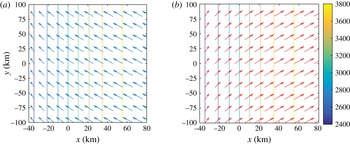
Let us first analyse the behaviour of the incoming HA wave away from the turning point. Figure 1( $a$ ) shows the contour plot of the bottom depth profile together with the vector plot of the wavenumber vector $\boldsymbol{k}_{n}^{-}(x)=\{-\unicode[STIX]{x1D707}_{n}(x),\unicode[STIX]{x1D6FC}_{n}\}$ for the incoming HA wave, for the first mode $n=1$ . Offshore of the turning point ( $x>x_{n}$ ), the water depth is greater than the critical depth ( $h>d_{n}$ ) and $\unicode[STIX]{x1D707}_{n}^{2}(x)>0$ , see (3.33). The wave field is oscillatory, the wavenumber vector $\boldsymbol{k}_{n}^{-}$ is oriented at approximately $138^{\circ }$ with respect to the $x$ axis (see right side of figure 1 $a$ ), with the incoming HA crests normal to $\boldsymbol{k}_{n}^{-}$ . Moving to shallower water towards the turning point ( $x\rightarrow x_{n}$ ), the water depth tends to the critical depth ( $h\rightarrow d_{n}$ ) and the offshore wavenumber of the incoming wave $\unicode[STIX]{x1D707}_{n}\rightarrow 0$ , see (3.33). However, the longshore wavenumber $\unicode[STIX]{x1D6FC}_{n}$ keeps constant following Snell’s law (3.16). As a result, $\boldsymbol{k}_{n}^{-}\rightarrow \{0,\unicode[STIX]{x1D6FC}_{n}\}$ as $h\rightarrow d_{n}$ , i.e. $\boldsymbol{k}_{n}^{-}$ decreases in magnitude and becomes increasingly parallel to the contours as the water depth decreases (see left side of figure 1 $a$ ). Because of (3.15), the crests become increasingly orthogonal to the depth contours. Note that this refraction dynamics is opposite to the refraction of gravity waves, where crests become increasingly parallel to the contours as $h$ decreases, see Mei et al. (Reference Mei, Stiassnie and Yue2005). At the turning point ( $x=x_{n}$ ) the incoming HA wave is refracted back to deeper water. The refracted wave is outgoing towards the far field and follows the pattern shown in figure 1(b) for $\boldsymbol{k}_{n}^{+}$ , exiting the domain at an angle $\unicode[STIX]{x1D703}_{n}^{+}\sim 42^{\circ }$ with respect to the $x$ axis. Clearly, the total HA wave field in the fluid domain is made up by the sum of incoming and refracted wave components.

Figure 1.

Contour plots of the bottom depth $h=3000+1000\tanh \,(2\times 10^{-5}x)$ , in metres, and vector plots of the wavenumber vector (3.19). ( $a$ ) Incoming wave: $\boldsymbol{k}_{n}^{-}(x)$ , (b) refracted wave: $\boldsymbol{k}_{n}^{+}(x)$ . The parameters are $n=1$ , $f=0.2~\text{Hz}$ and $\unicode[STIX]{x1D6FC}_{n}=5\times 10^{-4}~\text{m}^{-1}$ , which correspond to an angle of incidence of $138^{\circ }$ .

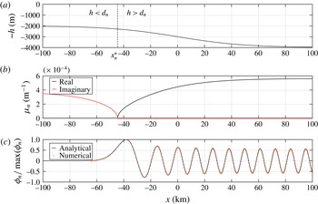
Close to the turning point $x_{n}=-44.5~\text{km}$ , (3.19) ceases to be valid. The behaviour of the HA waves must be analysed with the uniform asymptotic solution (3.36). Figure 2 shows a section of the sample bottom depth profile (figure 2 $a$ ), together with the behaviour of the slowly varying wavenumber $\unicode[STIX]{x1D707}_{n}$ (figure 2 $b$ ) and the uniform asymptotic solution $\unicode[STIX]{x1D719}_{n}(x,0)=X_{n}(x)$ (figure 2 $c$ ), for $n=1$ , over a long range along the offshore axis $x$ . Physically, the $\unicode[STIX]{x1D719}_{n}$ are exponentially decaying HA disturbances when the water depth is less than the critical depth ( $h<d_{n}$ for $x<x_{n}$ ), and the sum of incoming and refracted waves when the water depth is greater than the critical depth ( $h>d_{n}$ for $x>x_{n}$ ), as already shown in figure 1. Finally, we compared the asymptotic solution (3.36) to a fifth-order Runge–Kutta numerical solution of the governing equation (3.2), see figure 2(c). The agreement between the analytical approximation and the numerical results is excellent.

Figure 2.

(a) Bottom profile (solid line) and critical depth (vertical dashed line). (b) Real and imaginary part of the slowly varying wavenumber $\unicode[STIX]{x1D707}_{n}$ , expression (3.33). (c) Normalised mode $\unicode[STIX]{x1D719}_{n}/\max (\unicode[STIX]{x1D719}_{n})$ for $y=0$ , see (3.36). Parameters are $n=1$ , $f=0.2~\text{Hz}$ and $\unicode[STIX]{x1D6FC}_{n}=0.0005~\text{m}^{-1}$ .

Depth-dependent evanescent/propagating dynamics was also observed in two dimensions by Kadri & Stiassnie (Reference Kadri and Stiassnie2013) and Kadri (Reference Kadri2015). However, the results obtained in this paper are new for two main reasons. Mathematically, unlike the non-uniform result of Kadri & Stiassnie (Reference Kadri and Stiassnie2013), the uniform approximation (3.36) seamlessly connects the near and far fields, without the existence of a transition zone where the solution is not unique (see figure 2 of Kadri & Stiassnie Reference Kadri and Stiassnie2013). Physically, the 3-D propagation dynamics is significantly richer than that in two dimensions. In two dimensions, the topography of the seafloor controls the shoaling effects, by which the HA waves change height and group velocity as they propagate towards the shallows. Because of such effects, the $n$ th group velocity becomes null at the critical depth

(3.38) $$\begin{eqnarray}d_{n}^{(2D)}=\frac{(2n-1)\unicode[STIX]{x03C0}c}{2\unicode[STIX]{x1D714}},\end{eqnarray}$$

causing complete reflection of the relevant HA mode (Kadri & Stiassnie Reference Kadri and Stiassnie2013). Indeed, the same result is obtained from (3.32) in the 2-D limit $\unicode[STIX]{x1D6FC}_{n}=0$ . In three dimensions, on the other hand, the topography of the seafloor controls both shoaling and refraction effects. As a consequence, the HA waves change both height and direction as they propagate towards shallow water (see again figures 1 and 2). Hence, in three dimensions, each HA mode is not simply reflected back; instead, it gradually turns away as it approaches the shoreline (see figure 1 $a$ ), until the wavenumber component normal to the shoreline vanishes at the relevant critical depth $d_{n}$ , see (3.32). The latter defines the location where the $n$ th mode is refracted down the shelf. Unlike the 2-D limit (3.38), the critical depth in three dimensions (3.32) depends not only on the angular frequency $\unicode[STIX]{x1D714}$ of the incoming HA wave, but also on its longshore wavenumber $\unicode[STIX]{x1D6FC}_{n}$ . Expression (3.32) shows that the critical depth $d_{n}$ is minimum when $\unicode[STIX]{x1D6FC}_{n}=0$ (normal incidence, 2-D limit) and increases with increasing $\unicode[STIX]{x1D6FC}_{n}$ (oblique incidence). Physically, the larger the longshore component of the incoming HA wave, the less it penetrates towards the shore.

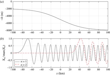
Concerning the higher-order HA modes, note that the critical depth (3.32) increases linearly with the modal order $n$ . Hence, higher-order modes are associated with greater critical depths and so propagate less onshore, as shown in figure 3. The latter shows the plot of the sample bottom depth $h(x)=5000+3000\,\tanh \,(2\times 10^{-5}x)$ (figure 3 $a$ ) together with the uniform asymptotic solutions $\unicode[STIX]{x1D719}_{n}(x,0)=X_{n}(x)$ for the first 2 HA modes (figure 3 $b$ ). The higher the modal order, the earlier the incoming HA mode is refracted down to deep water and the less it penetrates into shallower water.

Figure 3.

(a) Bottom profile for $h(x)=5000+3000\,\tanh \,(2\times 10^{-5}x)$ , in metres. (b) Normalised HA modes for $y=0$ , see (3.36). Parameters are $f=0.2~\text{Hz}$ and $\unicode[STIX]{x1D6FC}_{n}=0.0005~\text{m}^{-1}$ .

The refraction dynamics modelled by the MSEHA is in agreement with recent field measurements and numerical modelling of propagating HA waves in complex marine environments. As an example, Ballard (Reference Ballard2012) has investigated the horizontal refraction of low-frequency sound off the southeast coast of Florida. Ballard (Reference Ballard2012) has shown that, despite the sediment properties and the water-column sound-speed field exhibit significant range dependence over the shelf, the dynamics is almost exclusively controlled by the topography of the seafloor. Indeed, the results of Ballard (Reference Ballard2012) confirm that lower modes propagate further up the shelf and the location where they are refracted down to deep water is controlled by their critical depth (see again figure 3).

4.1 Analytical solution on a plane beach

Building on the free-wave results, let us now study how single HA frequencies, forced by a tsunamigenic disturbance at the bottom of the ocean, propagate over range-dependent environments. For the sake of example, consider the case of a plane beach of depth $h=\unicode[STIX]{x1D716}x$ , with $\unicode[STIX]{x1D716}\ll 1$ . Water is in the region $x>0$ , the shoreline is at $x=0$ . The plane beach geometry has important practical applications in tsunami models (Mei et al. Reference Mei, Stiassnie and Yue2005; Sammarco & Renzi Reference Sammarco and Renzi2008). It is also particularly interesting as it allows one to obtain an exact analytical solution in terms of integrals of Bessel functions. Following Mei et al. (Reference Mei, Stiassnie and Yue2005), consider a tsunamigenic bottom deformation, localised at $x=x_{0}$ :

(4.1) $$\begin{eqnarray}\bar{H}(\boldsymbol{x})=H_{0}\,\unicode[STIX]{x1D6FF}\left(\frac{x-x_{0}}{a}\right)\,\unicode[STIX]{x1D6FF}\left(\frac{y-0}{b}\right).\end{eqnarray}$$

In the latter, $\unicode[STIX]{x1D6FF}$ is the delta function, $x_{0}>0$ is the position of the centre of the perturbation along the $x$ axis, $H_{0}$ is the magnitude of the deformation, $a$ and $b$ are non-dimensionalising parameters. Results for generic disturbances can be found via the Green theorem (Mei et al. Reference Mei, Stiassnie and Yue2005). Symmetry of the perturbation (4.1) with respect to the $x$ axis allows us to use the cosine Fourier transform pair along the shoreline

(4.2a,b ) $$\begin{eqnarray}\hat{\unicode[STIX]{x1D719}}_{n}(x;\unicode[STIX]{x1D6FC})=\int _{0}^{\infty }\unicode[STIX]{x1D719}_{n}(x,y)\cos (\unicode[STIX]{x1D6FC}y)\,\text{d}y;\quad \unicode[STIX]{x1D719}_{n}(x,y)=\frac{2}{\unicode[STIX]{x03C0}}\int _{0}^{\infty }\hat{\unicode[STIX]{x1D719}}_{n}(x;\unicode[STIX]{x1D6FC})\cos (\unicode[STIX]{x1D6FC}y)\,\text{d}\unicode[STIX]{x1D6FC},\end{eqnarray}$$

so that the MSEHA (2.20) becomes

(4.3) $$\begin{eqnarray}\hat{\unicode[STIX]{x1D719}}_{n_{xx}}+\left[\frac{\unicode[STIX]{x1D714}^{2}}{c^{2}}-\unicode[STIX]{x1D6FC}^{2}-\frac{(2n-1)^{2}\unicode[STIX]{x03C0}^{2}}{4\unicode[STIX]{x1D716}^{2}x^{2}}\right]\hat{\unicode[STIX]{x1D719}}_{n}=-\frac{4}{\unicode[STIX]{x03C0}}\frac{(-1)^{n}}{2n-1}\text{i}\unicode[STIX]{x1D714}H_{0}b\,\unicode[STIX]{x1D6FF}\left(\frac{x-x_{0}}{a}\right)\sqrt{\frac{2}{\unicode[STIX]{x1D716}x}}.\end{eqnarray}$$

We shall now solve (4.3) with the method of patched matching (Bender & Orszag Reference Bender and Orszag1999). First, request that the solution be continuous at $x=x_{0}$ :

(4.4) $$\begin{eqnarray}\hat{\unicode[STIX]{x1D719}}_{n}(x_{0}+0;\unicode[STIX]{x1D6FC})=\hat{\unicode[STIX]{x1D719}}_{n}(x_{0}-0;\unicode[STIX]{x1D6FC}).\end{eqnarray}$$

Then, integrate (4.3) with respect to $x$ across the singularity at $x=x_{0}$ , to get

(4.5) $$\begin{eqnarray}\hat{\unicode[STIX]{x1D719}}_{n_{x}}(x_{0}+0;\unicode[STIX]{x1D6FC})-\hat{\unicode[STIX]{x1D719}}_{n_{x}}(x_{0}-0;\unicode[STIX]{x1D6FC})=-\frac{4}{\unicode[STIX]{x03C0}}\frac{(-1)^{n}}{2n-1}\text{i}\unicode[STIX]{x1D714}H_{0}\,a\,b\sqrt{\frac{2}{\unicode[STIX]{x1D716}x_{0}}}.\end{eqnarray}$$

The governing equation (4.3) is of the Bessel kind (Mei Reference Mei1997). The solution of (4.3) that satisfies the matching conditions (4.4) and (4.5) depends on the sign of $\unicode[STIX]{x1D6FC}-\unicode[STIX]{x1D714}/c$ . Again, we have two cases.

(i) $\unicode[STIX]{x1D6FC}>\unicode[STIX]{x1D714}/c$ . The solution is

(4.6) $$\begin{eqnarray}\hat{\unicode[STIX]{x1D719}}_{n}(x;\unicode[STIX]{x1D6FC})=\frac{4\sqrt{2}}{\unicode[STIX]{x03C0}}\frac{(-1)^{n}}{2n-1}\text{i}\unicode[STIX]{x1D714}H_{0}\frac{a\,b}{\unicode[STIX]{x1D716}}\,\sqrt{\unicode[STIX]{x1D716}x}~\text{K}_{\unicode[STIX]{x1D708}_{n}}\left(\sqrt{\unicode[STIX]{x1D6FC}^{2}-\frac{\unicode[STIX]{x1D714}^{2}}{c^{2}}}x_{0}\right)~\text{I}_{\unicode[STIX]{x1D708}_{n}}\left(\sqrt{\unicode[STIX]{x1D6FC}^{2}-\frac{\unicode[STIX]{x1D714}^{2}}{c^{2}}}x\right),\quad x<x_{0},\end{eqnarray}$$

for all points landward of the bottom disturbance, and

(4.7) $$\begin{eqnarray}\hat{\unicode[STIX]{x1D719}}_{n}(x;\unicode[STIX]{x1D6FC})=\frac{4\sqrt{2}}{\unicode[STIX]{x03C0}}\frac{(-1)^{n}}{2n-1}\text{i}\unicode[STIX]{x1D714}H_{0}\frac{a\,b}{\unicode[STIX]{x1D716}}\,\sqrt{\unicode[STIX]{x1D716}x}~\text{I}_{\unicode[STIX]{x1D708}_{n}}\left(\sqrt{\unicode[STIX]{x1D6FC}^{2}-\frac{\unicode[STIX]{x1D714}^{2}}{c^{2}}}x_{0}\right)~\text{K}_{\unicode[STIX]{x1D708}_{n}}\left(\sqrt{\unicode[STIX]{x1D6FC}^{2}-\frac{\unicode[STIX]{x1D714}^{2}}{c^{2}}}x\right),\quad x>x_{0},\end{eqnarray}$$

for all points offshore of the disturbance. In (4.6) and (4.7), $\text{I}_{\unicode[STIX]{x1D708}_{n}}$ and $\text{K}_{\unicode[STIX]{x1D708}_{n}}$ are, respectively, the modified Bessel functions of first and second kind and order $\unicode[STIX]{x1D708}_{n}$ , where

(4.8) $$\begin{eqnarray}\unicode[STIX]{x1D708}_{n}=\sqrt{\frac{1}{4}+\frac{(2n-1)^{2}\unicode[STIX]{x03C0}^{2}}{4\unicode[STIX]{x1D716}^{2}}}\sim \frac{(2n-1)\unicode[STIX]{x03C0}}{2\unicode[STIX]{x1D716}},\end{eqnarray}$$

for $\unicode[STIX]{x1D716}\ll 1$ . Recall that $\text{I}_{\unicode[STIX]{x1D708}_{n}}(z)\sim (0.5z)^{\unicode[STIX]{x1D708}_{n}}/\unicode[STIX]{x1D6E4}(\unicode[STIX]{x1D708}_{n}+1)$ as $z\rightarrow 0$ and $\text{K}_{\unicode[STIX]{x1D708}_{n}}(z)\sim \sqrt{\unicode[STIX]{x03C0}/(2z)}\exp (-z)$ as $z\rightarrow \infty$ , see Olver et al. (Reference Olver, Lozier, Boisvert and Clark2010). As a consequence, (4.6) yields $\hat{\unicode[STIX]{x1D719}}_{n}\rightarrow 0$ for $x\rightarrow 0$ and (4.7) gives $\hat{\unicode[STIX]{x1D719}}_{n}\rightarrow 0$ for $x\rightarrow \infty$ . Expressions (4.6)–(4.7) represent trapped HA waves that are important only in a strip near the bottom deformation.

(ii) $\unicode[STIX]{x1D6FC}<\unicode[STIX]{x1D714}/c$ . The solution is

(4.9) $$\begin{eqnarray}\hat{\unicode[STIX]{x1D719}}_{n}(x;\unicode[STIX]{x1D6FC})=-2\sqrt{2}\frac{(-1)^{n}}{2n-1}\unicode[STIX]{x1D714}H_{0}\frac{a\,b}{\unicode[STIX]{x1D716}}\sqrt{\unicode[STIX]{x1D716}x}~\text{H}_{\unicode[STIX]{x1D708}_{n}}\left(\sqrt{\frac{\unicode[STIX]{x1D714}^{2}}{c^{2}}-\unicode[STIX]{x1D6FC}^{2}}x_{0}\right)\text{J}_{\unicode[STIX]{x1D708}_{n}}\left(\sqrt{\frac{\unicode[STIX]{x1D714}^{2}}{c^{2}}-\unicode[STIX]{x1D6FC}^{2}}x\right),\quad x<x_{0},\end{eqnarray}$$

for all points landward of the bottom disturbance, and

(4.10) $$\begin{eqnarray}\hat{\unicode[STIX]{x1D719}}_{n}(x;\unicode[STIX]{x1D6FC})=-2\sqrt{2}\frac{(-1)^{n}}{2n-1}\unicode[STIX]{x1D714}H_{0}\frac{a\,b}{\unicode[STIX]{x1D716}}\sqrt{\unicode[STIX]{x1D716}x}~\text{J}_{\unicode[STIX]{x1D708}_{n}}\left(\sqrt{\frac{\unicode[STIX]{x1D714}^{2}}{c^{2}}-\unicode[STIX]{x1D6FC}^{2}}x_{0}\right)\text{H}_{\unicode[STIX]{x1D708}_{n}}\left(\sqrt{\frac{\unicode[STIX]{x1D714}^{2}}{c^{2}}-\unicode[STIX]{x1D6FC}^{2}}x\right),\quad x>x_{0},\end{eqnarray}$$

for all points offshore of the disturbance. In (4.9) and (4.10), $\text{J}_{\unicode[STIX]{x1D708}_{n}}$ and $\text{H}_{\unicode[STIX]{x1D708}_{n}}$ are, respectively, the Bessel and the Hankel functions of the first kind. Recall that $\text{J}_{\unicode[STIX]{x1D708}_{n}}(z)\sim (0.5z)^{\unicode[STIX]{x1D708}_{n}}/\unicode[STIX]{x1D6E4}(\unicode[STIX]{x1D708}_{n}+1)$ as $z\rightarrow 0$ , see Olver et al. (Reference Olver, Lozier, Boisvert and Clark2010). As a consequence, (4.9) yields $\hat{\unicode[STIX]{x1D719}}_{n}\rightarrow 0$ for $x\rightarrow 0$ , i.e. $\hat{\unicode[STIX]{x1D719}}_{n}$ decays towards the shoreline. On the other hand, the function $\text{H}_{\unicode[STIX]{x1D708}_{n}}$ in (4.10) is outgoing as $x\rightarrow \infty$ . Therefore, (4.9)–(4.10) describe HA waves that decay near the shoreline and propagate towards the far field. Finally, substitution of (4.6)–(4.10) inside the inverse cosine Fourier transform (4.2), together with the decomposition (2.8), yields the $n$ th spatial HA potential

(4.11) $$\begin{eqnarray}\bar{\unicode[STIX]{x1D6F7}}_{n}(\boldsymbol{x},z)=\bar{\unicode[STIX]{x1D6F7}}_{n}^{t}(\boldsymbol{x},z)+\bar{\unicode[STIX]{x1D6F7}}_{n}^{p}(\boldsymbol{x},z).\end{eqnarray}$$

In the latter,

(4.12) $$\begin{eqnarray}\displaystyle \bar{\unicode[STIX]{x1D6F7}}_{n}^{t}(\boldsymbol{x},z) & = & \displaystyle \frac{16}{\unicode[STIX]{x03C0}^{2}}\frac{(-1)^{n}}{2n-1}\text{i}\unicode[STIX]{x1D714}H_{0}\frac{a\,b}{\unicode[STIX]{x1D716}}\cos \left[(2n-1)\frac{\unicode[STIX]{x03C0}}{2}\left(1+\frac{z}{\unicode[STIX]{x1D716}x}\right)\right]\nonumber\\ \displaystyle & & \displaystyle \times \,\int _{\unicode[STIX]{x1D714}/c}^{\infty }\left[\text{K}_{\unicode[STIX]{x1D708}_{n}}\left(\sqrt{\unicode[STIX]{x1D6FC}^{2}-\frac{\unicode[STIX]{x1D714}^{2}}{c^{2}}}x_{0}\right)\text{I}_{\unicode[STIX]{x1D708}_{n}}\left(\sqrt{\unicode[STIX]{x1D6FC}^{2}-\frac{\unicode[STIX]{x1D714}^{2}}{c^{2}}}x\right)H_{e}(x_{0}-x)\right.\,\nonumber\\ \displaystyle & & \displaystyle +\,\left.\text{I}_{\unicode[STIX]{x1D708}_{n}}\left(\sqrt{\unicode[STIX]{x1D6FC}^{2}-\frac{\unicode[STIX]{x1D714}^{2}}{c^{2}}}x_{0}\right)\text{K}_{\unicode[STIX]{x1D708}_{n}}\left(\sqrt{\unicode[STIX]{x1D6FC}^{2}-\frac{\unicode[STIX]{x1D714}^{2}}{c^{2}}}x\right)H_{e}(x-x_{0})\right]\cos (\unicode[STIX]{x1D6FC}y)\,\text{d}\unicode[STIX]{x1D6FC}\nonumber\\ \displaystyle & & \displaystyle\end{eqnarray}$$

is the trapped component, where $H_{e}$ is the Heaviside step function, while

(4.13) $$\begin{eqnarray}\displaystyle \bar{\unicode[STIX]{x1D6F7}}_{n}^{p}(\boldsymbol{x},z) & = & \displaystyle -\frac{8}{\unicode[STIX]{x03C0}}\frac{(-1)^{n}}{2n-1}\unicode[STIX]{x1D714}H_{0}\frac{a\,b}{\unicode[STIX]{x1D716}}\cos \left[(2n-1)\frac{\unicode[STIX]{x03C0}}{2}\left(1+\frac{z}{\unicode[STIX]{x1D716}x}\right)\right]\nonumber\\ \displaystyle & & \displaystyle \times \int _{0}^{\unicode[STIX]{x1D714}/c}\left[\text{H}_{\unicode[STIX]{x1D708}_{n}}\left(\sqrt{\frac{\unicode[STIX]{x1D714}^{2}}{c^{2}}-\unicode[STIX]{x1D6FC}^{2}}x_{0}\right)\text{J}_{\unicode[STIX]{x1D708}_{n}}\left(\sqrt{\frac{\unicode[STIX]{x1D714}^{2}}{c^{2}}-\unicode[STIX]{x1D6FC}^{2}}x\right)H_{e}(x_{0}-x)\right.\,\nonumber\\ \displaystyle & & \displaystyle +\left.\text{J}_{\unicode[STIX]{x1D708}_{n}}\left(\sqrt{\frac{\unicode[STIX]{x1D714}^{2}}{c^{2}}-\unicode[STIX]{x1D6FC}^{2}}x_{0}\right)\text{H}_{\unicode[STIX]{x1D708}_{n}}\left(\sqrt{\frac{\unicode[STIX]{x1D714}^{2}}{c^{2}}-\unicode[STIX]{x1D6FC}^{2}}x\right)H_{e}(x-x_{0})\right]\cos (\unicode[STIX]{x1D6FC}y)\,\text{d}\unicode[STIX]{x1D6FC}\nonumber\\ \displaystyle & & \displaystyle\end{eqnarray}$$

is the propagating component. Hence the tsunamigenic bottom disturbance (4.1) generates a twofold HA wave field, made by trapped components (4.12) and progressive components which propagate offshore, but decay towards the shoreline (4.13). This happens precisely because the HA frequencies turn away as they approach the shore (see again § 3). The dynamic pressure can be determined from the HA potential with the expression $p_{n}(\boldsymbol{x},z,t)=-\unicode[STIX]{x1D70C}_{0}\unicode[STIX]{x1D6F7}_{n_{t}}$ (see Renzi & Dias Reference Renzi and Dias2014a ), which yields $p_{n}(\boldsymbol{x},z,t)=p_{n}^{t}(\boldsymbol{x},z,t)+p_{n}^{p}(\boldsymbol{x},z,t)$ . In the latter,

(4.14) $$\begin{eqnarray}p_{n}^{(t,p)}(\boldsymbol{x},z,t)=\text{Re}\,\left\{\text{i}\unicode[STIX]{x1D70C}_{0}\unicode[STIX]{x1D714}\,\bar{\unicode[STIX]{x1D6F7}}_{n}^{(t,p)}(\boldsymbol{x},z)\,\text{e}^{-\text{i}\unicode[STIX]{x1D714}t}\right\}\end{eqnarray}$$

is the dynamic pressure of the $n$ th trapped (propagating) HA component. Finally, we define the transmission loss as

(4.15) $$\begin{eqnarray}\text{TL}=-20\log _{10}\left|\frac{\bar{p}(\boldsymbol{x},z)}{p_{0}(r=1~\text{m})}\right|,\end{eqnarray}$$

where $\bar{p}(\boldsymbol{x},z)=\text{i}\unicode[STIX]{x1D70C}_{0}\unicode[STIX]{x1D714}\,\bar{\unicode[STIX]{x1D6F7}}(\boldsymbol{x},z)$ is the spatial component of the total pressure generated by the bottom disturbance and

(4.16) $$\begin{eqnarray}p_{0}(r)=\unicode[STIX]{x1D70C}_{0}\unicode[STIX]{x1D714}^{2}H_{0}ab\,\frac{\exp (\text{i}\unicode[STIX]{x1D714}r/c)}{4\unicode[STIX]{x03C0}r}\end{eqnarray}$$

is the pressure produced at a distance $r$ by a source of the same intensity as the bottom disturbance, but in an infinite, homogeneous medium with the ambient density $\unicode[STIX]{x1D70C}_{0}$ (Jensen et al. Reference Jensen, Kuperman, Porter and Schmidt2011).

4.2 Numerical example

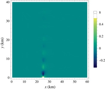
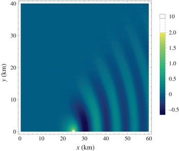
Let us now analyse the propagation of HA waves generated by a tsunamigenic disturbance at the bottom of a plane beach. For simplicity, we shall consider a unit volume displacement, i.e. $a=b=H_{0}=1~\text{m}$ , so that the results will be per unit $\text{m}^{3}$ of displaced volume. The bottom slope is $\unicode[STIX]{x1D716}=0.08$ . Figure 4 shows the density plot of the pressure $p_{n}^{t}$ of the trapped HA component (4.14) of frequency $f=0.2~\text{Hz}$ and modal order $n=1$ at the bottom of the ocean, $z=-\unicode[STIX]{x1D716}x$ , generated by the bottom disturbance at $x_{0}=25~\text{km}$ from the shoreline, at a depth $h_{0}=2~\text{km}$ . This choice of parameters is consistent with the 1693 East Mediterranean earthquake scenario studied by Cecioni et al. (Reference Cecioni, Abdolali, Bellotti and Sammarco2015), in which the signal generated at a depth $h=2~\text{km}$ has a carrier frequency of $f\sim 0.2~\text{Hz}$ . Figure 4 shows that the trapped component decays either onshore and offshore along the $x$ axis, but propagates parallel to the shoreline. Note that the trapped component is not refracted, because it has not a progressive wave structure along $x$ . The plot of the full dynamic pressure $p_{n}=p_{n}^{t}+p_{n}^{p}$ is shown in figure 5. The signal mostly propagates from the generation point towards deeper water in the form of outgoing progressive waves. This means that the dynamics away from the source is dominated by the propagating component $p_{n}^{p}$ , which is stronger than the trapped longshore component $p_{n}^{t}$ of figure 4. Figure 5 also reveals that shorter HA waves travel faster, followed by a tail of longer waves (see also Yamamoto Reference Yamamoto1982; Renzi & Dias Reference Renzi and Dias2014b ). This is opposite to the dispersive behaviour of gravity waves (Mei et al. Reference Mei, Stiassnie and Yue2005). Finally, note that the refraction effects discussed in § 3 limit the transmission of the signal towards the shore.

Figure 4.

Pressure $p_{n}^{t}$ of the trapped HA component at the bottom of a plane beach, $z=-\unicode[STIX]{x1D716}x$ , generated by a bottom disturbance located at $x_{0}=25~\text{km}$ from the shoreline; $x$ and $y$ denote the offshore and longshore directions, respectively. The parameters are $n=1$ , $f=0.2~\text{Hz}$ , $\unicode[STIX]{x1D716}=0.08$ , $a=b=H_{0}=1~\text{m}$ . Pressure values are in $\text{Pa}~\text{m}^{-3}$ of displaced volume. Values are clipped near the source for easiness of reading.

Figure 5.

Dynamic pressure $p_{n}=p_{n}^{t}+p_{n}^{p}$ at the bottom of a plane beach, generated by a bottom disturbance at $x_{0}=25~\text{km}$ . The parameters are the same as in figure 4. Pressure values are in $\text{Pa}~\text{m}^{-3}$ of displaced volume. Values are clipped near the source for easiness of reading.

We have also analysed the behaviour of higher modes. Already for $n=2$ , the dynamic pressure $p_{n}$ is noticeable only in a very small region near the source and then vanishes quickly away from it. This agrees with the results of Stiassnie (Reference Stiassnie2010), who found that the first mode carries most of the energy transferred by the bottom motion to the HA waves. Equally, Eyov et al. (Reference Eyov, Klar, Kadri and Stiassnie2013), Hendin & Stiassnie (Reference Hendin and Stiassnie2013), Cecioni et al. (Reference Cecioni, Abdolali, Bellotti and Sammarco2015) and Kadri (Reference Kadri2015) showed that the first HA mode has the largest amplitude and contains most of the energy. As a consequence, the higher modes $n>1$ do not influence the transmission loss (4.15) away from the source.

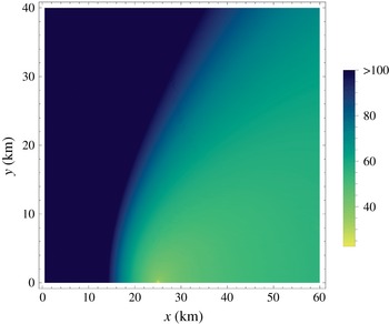
Figure 6 shows the transmission loss (TL) at the bottom of the fluid domain, $z=-\unicode[STIX]{x1D716}x$ . The plot highlights the existence of a shadow zone where TL is maximum and the signal is strongly attenuated. This result explains the interesting observations of Cecioni et al. (Reference Cecioni, Abdolali, Bellotti and Sammarco2015) on the numerical simulation of the AD 365 Eastern Mediterranean earthquake. Cecioni et al. (Reference Cecioni, Abdolali, Bellotti and Sammarco2015) noted that the HA perturbation generated by the earthquake off western Crete could not reach the shallower water areas south-west of Sicily, even after long time from the earthquake, despite the associated tsunami did hit Sicily. Cecioni et al. (Reference Cecioni, Abdolali, Bellotti and Sammarco2015) hypothesised a filtering effect of the water depth as the cause of the phenomenon. The analytical solution of the MSEHA further clarifies the reason of this dynamics: refraction turns the propagating HA wave frequencies down to deep water, preventing them from reaching the shallows, where indeed the transmission loss is maximum (see again figure 6).

Figure 6.

Transmission loss $\text{TL}$  (4.15) at the bottom of a plane beach generated by a bottom disturbance at $x_{0}=25~\text{km}$ . The parameters are the same as in figure 4. Transmission loss values are in $\text{dB}$ re 1 m.