2. Dynamic excess kurtosis

Drawing on Janssen (Reference Janssen2003) the dynamic excess kurtosis of weakly nonlinear sea states, initially homogeneous and Gaussian, is given by

(2.1) $$\begin{eqnarray}C_{4}^{d}=\frac{4g}{{\it\sigma}^{2}}\text{Re}\int T_{12}^{34}{\it\delta}_{12}^{34}\sqrt{\frac{{\it\omega}_{4}}{{\it\omega}_{1}{\it\omega}_{2}{\it\omega}_{3}}}G(t)E_{1}E_{2}E_{3}\,\text{d}{\it\omega}_{1,2,3}\,\text{d}{\it\theta}_{1,2,3},\end{eqnarray}$$

where the resonant function

(2.2) $$\begin{eqnarray}G(t)=\frac{1-\exp (-\text{i}{\it\omega}_{12}^{34}t)}{{\it\omega}_{12}^{34}},\end{eqnarray}$$

$T_{12}^{34}$ is the Zakharov kernel (Zakharov Reference Zakharov1968, Reference Zakharov1999; Krasitskii Reference Krasitskii1994) as a function of the wavenumber vectors $\boldsymbol{k}_{j}=(k_{j}\cos ({\it\theta}_{j}),k_{j}\sin ({\it\theta}_{j}))$ and $\text{Re}(x)$ denotes the real part of  $x$ . The sixfold integral in (2.1) is defined over the manifold

(2.3) $$\begin{eqnarray}\boldsymbol{k}_{1}+\boldsymbol{k}_{2}-\boldsymbol{k}_{3}-\boldsymbol{k}_{4}=\mathbf{0}\end{eqnarray}$$

or equivalently ${\it\delta}_{12}^{34}={\it\delta}(\boldsymbol{k}_{1}+\boldsymbol{k}_{2}-\boldsymbol{k}_{3}-\boldsymbol{k}_{4})$ , where ${\it\delta}(\boldsymbol{k})$ is the Dirac delta. The frequency mismatch is given by ${\it\omega}_{12}^{34}={\it\omega}_{1}+{\it\omega}_{2}-{\it\omega}_{3}-{\it\omega}_{4}$ , $E({\it\omega},{\it\theta})$ is the surface spectrum and ${\it\sigma}^{2}$ is the variance of surface elevations. The deep-water angular frequency ${\it\omega}(k)=\sqrt{gk}$ , the wavenumber magnitude $k=|\boldsymbol{k}|$ , and

(2.4) $$\begin{eqnarray}\displaystyle {\it\omega}_{4}=\sqrt{gk_{4}}=\sqrt{g|\boldsymbol{k}_{1}+\boldsymbol{ k}_{2}-\boldsymbol{ k}_{3}|} & & \displaystyle\end{eqnarray}$$

follows from (2.3), with $g$ denoting gravity acceleration. Since homogeneous Gaussian initial conditions with random phases and amplitudes are imposed, it follows that

(2.5) $$\begin{eqnarray}\displaystyle C_{4}^{d}(t=0)=0. & & \displaystyle\end{eqnarray}$$

Equation (2.1) can be simplified by resorting to a narrowband approximation (Mori & Janssen Reference Mori and Janssen2006; Janssen & Bidlot Reference Janssen and Bidlot2009). So, we assume the spectrum $E$ to peak at ${\it\omega}={\it\omega}_{0}$ and ${\it\theta}={\it\theta}_{0}$ , where ${\it\omega}_{0}$ and ${\it\theta}_{0}$ denote the dominant angular frequency and wave direction, respectively, and the associated wavenumber $k_{0}={\it\omega}_{0}^{2}/g$ , wave period $T_{0}=2{\rm\pi}/{\it\omega}_{0}$ and phase speed $c_{0}={\it\omega}_{0}/k_{0}$ . Next, define

(2.6a,b ) $$\begin{eqnarray}\displaystyle {\it\omega}_{j}={\it\omega}_{0}(1+{\it\nu}v_{j}),\quad {\it\theta}_{j}={\it\theta}_{0}+{\it\sigma}_{{\it\theta}}{\it\phi}_{j}, & & \displaystyle\end{eqnarray}$$

where ${\it\nu}$ and ${\it\sigma}_{{\it\theta}}$ denote spectral and angular widths respectively. Under the narrowband condition ${\it\nu},{\it\sigma}_{{\it\theta}}\ll 1$ , $T_{12}^{34}\sim k_{0}^{3}$ to leading order and the frequency mismatch, correct to $O({\it\nu}^{2},{\it\sigma}_{{\it\theta}}^{2})$ , is given by

(2.7) $$\begin{eqnarray}{\it\omega}_{12}^{34}\sim {\it\nu}^{2}{\it\omega}_{0}{\it\Delta},\end{eqnarray}$$

with

(2.8) $$\begin{eqnarray}\displaystyle {\it\Delta}=\{(v_{1}-v_{3})(v_{2}-v_{3})-R({\it\phi}_{1}-{\it\phi}_{3})({\it\phi}_{2}-{\it\phi}_{3})\}={\it\Delta}_{v}-R{\it\Delta}_{{\it\phi}}, & & \displaystyle\end{eqnarray}$$

where ${\it\Delta}_{z}=(z_{1}-z_{3})(z_{2}-z_{3})$ for a generic $z=(z_{1},z_{2},z_{3})$ triplet, and the parameter

(2.9) $$\begin{eqnarray}R=\frac{1}{2}\frac{{\it\sigma}_{{\it\theta}}^{2}}{{\it\nu}^{2}}\end{eqnarray}$$

is a measure of short-crestedness of dominant waves (Janssen & Bidlot Reference Janssen and Bidlot2009). Expanding (2.1) around ${\it\nu}=0$ and ${\it\sigma}_{{\it\theta}}=0$ , to leading order

(2.10) $$\begin{eqnarray}C_{4}^{d}({\it\tau})=\text{BFI}^{2}J({\it\tau};R),\end{eqnarray}$$

where

(2.11) $$\begin{eqnarray}J({\it\tau};R)=2\,\text{Re}\int \frac{1-\exp (\text{i}{\it\Delta}{\it\tau})}{{\it\Delta}}\widetilde{E}_{1}\widetilde{E}_{2}\widetilde{E}_{3}\,\text{d}v_{1,2,3}\,\text{d}{\it\phi}_{1,2,3}.\end{eqnarray}$$

Here, ${\it\tau}={\it\nu}^{2}{\it\omega}_{0}t$ is a dimensionless time and $\widetilde{E}_{j}(v_{j},{\it\phi}_{j})=E_{j}/{\it\sigma}$ .

For a Gaussian-shaped spectrum, the rate of change of $C_{4}^{d}$ is explicitly given by

(2.12) $$\begin{eqnarray}\frac{\text{d}C_{4}^{d}}{\text{d}{\it\tau}}=\text{BFI}^{2}\frac{\text{d}J}{\text{d}{\it\tau}},\end{eqnarray}$$

and

(2.13) $$\begin{eqnarray}\frac{\text{d}J}{\text{d}{\it\tau}}=\frac{\text{d}J_{0}({\it\tau};1,R)}{\text{d}{\it\tau}}=2\,\text{Im}\left(\frac{1}{\sqrt{1-2\text{i}{\it\tau}+3{\it\tau}^{2}}\sqrt{1+2\text{i}R{\it\tau}+3R^{2}{\it\tau}^{2}}}\right),\end{eqnarray}$$

where the function $J_{0}({\it\tau};P,Q)$ is defined in appendix A and $\text{Im}(x)$ denotes the imaginary part of $x$ . On this basis, the factor $J$ in (2.10) follows by quadrature as

(2.14) $$\begin{eqnarray}J({\it\tau};R)=2\,\text{Im}\int _{0}^{{\it\tau}}\frac{1}{\sqrt{1-2\text{i}{\it\alpha}+3{\it\alpha}^{2}}\sqrt{1+2\text{i}R{\it\alpha}+3R^{2}{\it\alpha}^{2}}}\,\text{d}{\it\alpha}.\end{eqnarray}$$

For small times ${\it\tau}\ll 1$ ,

(2.15) $$\begin{eqnarray}\displaystyle J({\it\tau};R)=\int _{0}^{{\it\tau}}((1-R){\it\alpha}+O({\it\alpha}^{2}))\,\text{d}{\it\alpha}=\frac{1}{2}(1-R){\it\tau}^{2} & & \displaystyle\end{eqnarray}$$

and (2.10) yields

(2.16) $$\begin{eqnarray}C_{4}^{d}\sim \text{BFI}^{2}(1-R){\it\tau}^{2},\quad {\it\tau}\ll 1,\end{eqnarray}$$

in agreement with Janssen & Bidlot (Reference Janssen and Bidlot2009).

Note that the dynamic excess kurtosis in (2.10) is consistent with the evolution of weakly nonlinear narrowband wavetrains of the two-dimensional (2-D) NLS equation.

3. Intrinsic nonlinear time scale

The growth rate (2.12) of the dynamic $C_{4}^{d}$ vanishes at the dimensionless time

(3.1) $$\begin{eqnarray}{\it\tau}_{c}=\frac{1}{\sqrt{3R}},\end{eqnarray}$$

or in physical units

(3.2) $$\begin{eqnarray}\frac{t_{c}}{T_{0}}=\frac{1}{2{\rm\pi}}\sqrt{\frac{2}{3}}\frac{1}{{\it\sigma}_{{\it\theta}}{\it\nu}}\sim \frac{0.13}{{\it\sigma}_{{\it\theta}}{\it\nu}},\end{eqnarray}$$

where $T_{0}=2{\rm\pi}/{\it\omega}_{0}$ is the dominant wave period. Further, the second derivative of $C_{4}^{d}$ at ${\it\tau}_{c}$ is given by

(3.3) $$\begin{eqnarray}\displaystyle \left.\frac{\text{d}^{2}C_{4}^{d}}{\text{d}{\it\tau}^{2}}\right|_{{\it\tau}={\it\tau}_{c}}=-6\sqrt{3}R(1-R). & & \displaystyle\end{eqnarray}$$

Thus, $C_{4}^{d}$ attains a positive maximum (negative minimum) at ${\it\tau}={\it\tau}_{c}$ for $0<R<1$ ( $R>1$ ). It is straightforward to show that for multidirectional or short-crested seas ( $R>0$ )

(3.4) $$\begin{eqnarray}\displaystyle \mathop{\text{lim}}_{{\it\tau}\rightarrow \infty }C_{4}^{d}=0. & & \displaystyle\end{eqnarray}$$

Indeed, it is sufficient to study the rate of change of $C_{4}^{d}$ for large times ${\it\tau}\gg 1$ . To do so, consider the change of variable ${\it\tau}=1/r$ and expanding (2.12) around $r=0$ yields

(3.5) $$\begin{eqnarray}\frac{\text{d}C_{4}^{d}}{\text{d}{\it\tau}}\sim \frac{(-1+R)r^{3}}{9R^{2}}=\frac{(-1+R)}{9R^{2}{\it\tau}^{3}}.\end{eqnarray}$$

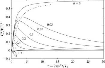
Note that in (2.13) the real part of the term within parentheses, which has no physical meaning, decays as ${\it\tau}^{-2}$ . For $0<R<1$ , $C_{4}^{d}$ first attains a positive peak at ${\it\tau}={\it\tau}_{c}$ and then decays monotonically to zero since $\text{d}C_{4}^{d}/\text{d}{\it\tau}<0$ for large ${\it\tau}$ . This is clearly seen in figure 1, showing the evolution of $C_{4}^{d}$ for different values of $R$ . For $R>1$ , $C_{4}^{d}$ initially decreases, reaching a negative peak at ${\it\tau}={\it\tau}_{c}$ , and then tends monotonically to zero, because $\text{d}C_{4}^{d}/\text{d}{\it\tau}>0$ for large ${\it\tau}$ as shown in figure 1. At the critical value $R=1$ , the excess kurtosis is null at any time, as can easily be verified from (2.12).

In summary, depending on the value of $R$ there will be nonlinear focusing ( $C_{4}^{d}>0$ ) or nonlinear defocusing ( $C_{4}^{d}<0$ ) in agreement with Janssen & Bidlot (Reference Janssen and Bidlot2009). Note that for unidirectional or long-crested seas ( $R=0$ ) the rate of change $\text{d}C_{4}^{d}/\text{d}{\it\tau}>0$ for any time ${\it\tau}$ . In this case, the dynamic excess kurtosis monotonically increases with time to the asymptotic value of (1.4) (Mori & Janssen Reference Mori and Janssen2006; Shemer & Sergeeva Reference Shemer and Sergeeva2009; Fedele et al. Reference Fedele, Cherneva, Tayfun and Soares2010; Shemer et al. Reference Shemer, Sergeeva and Liberzon2010a ,Reference Shemer, Sergeeva and Slunyaev b ).

Figure 1.

Dynamic excess kurtosis: solid lines, $C_{4}^{d}/\text{BFI}^{2}$ as a function of dimensionless time ${\it\tau}={\it\nu}^{2}{\it\omega}_{0}t=2{\rm\pi}{\it\nu}^{2}t/T_{0}$ for different values of $R$ ; dashed line, locus of transient peaks ( $T_{0}$ denotes the dominant wave period and ${\it\nu}$ is the spectral bandwidth).

4. Dynamic excess kurtosis maximum

From (2.10) and (3.1), the peak value of $C_{4}^{d}$ at ${\it\tau}={\it\tau}_{c}$ is given by

(4.1) $$\begin{eqnarray}C_{4}^{d}(R)=\text{BFI}^{2}J_{p}(R),\end{eqnarray}$$

where

(4.2) $$\begin{eqnarray}\displaystyle J_{p}(R)=J\left(\frac{1}{\sqrt{3R}};R\right)=\text{Im}\int _{0}^{1/\sqrt{3R}}\frac{2}{\sqrt{1-2\text{i}{\it\alpha}+3{\it\alpha}^{2}}\sqrt{1+2\text{i}R{\it\alpha}+3R^{2}{\it\alpha}^{2}}}\,\text{d}{\it\alpha}. & & \displaystyle\end{eqnarray}$$

The following relation holds:

(4.3) $$\begin{eqnarray}\displaystyle J_{p}\left(\frac{1}{R}\right)=-RJ_{p}(R), & & \displaystyle\end{eqnarray}$$

in agreement with Janssen & Bidlot (Reference Janssen and Bidlot2009). This relation allows us to compute the minimum kurtosis for $R>1$ from the maximum value for $R<1$ . Indeed,

(4.4) $$\begin{eqnarray}C_{4,min}^{d}\left(\frac{1}{R}\right)=-RC_{4,max}^{d}(R),\quad 0\leqslant R\leqslant 1,\end{eqnarray}$$

where $C_{4,max}^{d}=\text{BFI}^{2}J_{p}(R)$ . Clearly, this vanishes at $R=1$ signalling the change from a nonlinear focusing to a defocusing regime where the dynamic excess kurtosis is negative.

Drawing on Janssen & Bidlot (Reference Janssen and Bidlot2009), the limit

(4.5) $$\begin{eqnarray}J_{p}(R)\sim -\frac{{\rm\pi}}{3\sqrt{3}R},\quad R\gg 1,\end{eqnarray}$$

and that for small times in (2.16), suggest the least-squares fit for the maximum

(4.6) $$\begin{eqnarray}\frac{C_{4,max}^{d}(R)}{\text{BFI}^{2}}=J_{peak}(R)\approx \frac{b}{(2{\rm\pi})^{2}}\frac{1-R}{R+bR_{0}},\quad 0\leqslant R\leqslant 1,\end{eqnarray}$$

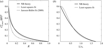
where $R_{0}=(3\sqrt{3})/{\rm\pi}$ and $b=2.48$ . In figure 2(a), the preceding approximation is compared to the theoretical $C_{4,max}^{d}$ obtained from solving (4.1) by numerical integration. Evidently, the latter is slightly larger than the maximum excess kurtosis derived by Janssen & Bidlot (Reference Janssen and Bidlot2009), who have also used (4.6) but with $b=1$ . Their maximum follows by first taking the limit of the resonant function $G(t)$ in (2.2) at $t=\infty$ and then solving the sixfold integral in (2.1). Clearly, for $R>0$ the dynamic excess kurtosis should vanish at large times as discussed above. Janssen (personal communication, Reference Janssen2014a ) confirmed that (4.1) holds and provided an alternative proof that $C_{4}^{d}$ tends to zero as $t\rightarrow \infty$ using complex analysis and numerical integration.

Further, from (3.1)

(4.7) $$\begin{eqnarray}\frac{C_{4,max}^{d}({\it\tau}_{c})}{\text{BFI}^{2}}\approx \frac{b}{(2{\rm\pi})^{2}}\frac{-1+3{\it\tau}_{c}^{2}}{1+3bR_{0}{\it\tau}_{c}^{2}},\quad 0\leqslant {\it\tau}_{c}\leqslant \frac{1}{\sqrt{3}}.\end{eqnarray}$$

Clearly, the transient maximum kurtosis becomes larger for longer time scales ${\it\tau}_{c}$ , as illustrated in figure 2(b). Note that the dynamic excess kurtosis is negative for ${\it\tau}_{c}>1/\sqrt{3}$ as the wave regime is of defocusing type ( $R>1$ ) and the minimum value $C_{4,min}^{d}$ can be computed from (4.4).

Figure 2.

Maximum dynamic excess kurtosis $C_{4,max}^{d}$ as a function of (a) $R$ and (b) $1/{\it\tau}_{c}$ : bold line, present theoretical prediction; thin line, least-squares fit from (4.6) ( $b=2.48$ ); dashed line, Janssen & Bidlot (Reference Janssen and Bidlot2009) fit ( $b=1$ ).

5. Comparisons to simulations and experiments

We now compare the theoretical narrowband (NB) predictions for the total kurtosis $C_{4}$ (see (1.2), (2.10) and (1.3)) to experimental results (Onorato et al. Reference Onorato, Cavaleri, Fouques, Gramstad, Janssen, Monbaliu, Osborne, Pakozdi, Serio, Stansberg, Toffoli and Trulsen2009) and the comprehensive numerical simulations of JONSWAP directional wave fields carried out by Toffoli et al. (Reference Toffoli, Gramstad, Trulsen, Monbaliu, Bitner-Gregersen and Onorato2010) and Xiao et al. (Reference Xiao, Liu, Wu and Yue2013). They considered the broadband modified nonlinear Schrödinger equations (BMNLS) (Dysthe Reference Dysthe1979) and a high-order spectral (HOS) solver (Dommermuth & Yue Reference Dommermuth and Yue1987). In particular, we consider the comprehensive numerical results reported in figures 10(a,b) in Xiao et al. (Reference Xiao, Liu, Wu and Yue2013) for the two cases of narrow and broad directional spreading, i.e. ${\it\sigma}_{{\it\theta}}=0.04$ and 0.07 respectively. 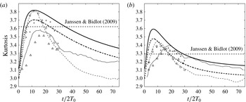The simulated sea states have standard deviation ${\it\sigma}=0.02\;\text{m}$ , dominant wave period $T_{0}=1\;\text{s}$ , significant wave height $H_{s}=4{\it\sigma}=0.08\;\text{m}$ , $\text{BFI}=0.78$ , wave steepness ${\it\mu}=0.08$ and spectral bandwidth ${\it\nu}=0.15$ (see appendix B for the estimation of wave parameters). As shown in figure 3, the numerical studies by Xiao et al. (Reference Xiao, Liu, Wu and Yue2013) indicate an initial overshoot of the kurtosis followed by a decay towards quasi-Gaussian conditions.

In particular, figure 3(a) shows that for a narrow directional spreading ( ${\it\sigma}_{{\it\theta}}\sim 0.04$ ) the present theoretical NB model (thick line) explains the peak kurtosis and the initial transient behaviour of BMNLS simulations (thin dashed line) as NB is consistent with the dynamics of the 2-D NLS equation. BMNLS and NB yield faster initial growth and overestimate both HOS (thin solid line) and experiments (triangle symbols). However, soon after the transient stage, the spectrum has already broadened in frequency and spread angularly, approaching a quasi-equilibrium state. At this stage, the NB approximation provides just a qualitative trend of the large-time behaviour since it does not account for spectral changes. In particular, NB shows a slower decaying trend to zero than BMNLS. This indicates that numerical models capture the directional energy spreading and quasi-resonant interactions attenuate much faster than NB after the transient peak.

For a broad directional spreading ( ${\it\sigma}_{{\it\theta}}\sim 0.07$ ) figure 3(b) shows that NB overestimates the maximum kurtosis and qualitatively explains the initial transient overshoot of BMNLS simulations, which are now beyond their range of validity as the spectrum is already too broad initially. Instead, HOS simulations are in agreement with experiments and yield a smaller value of the maximum kurtosis and a slower transient than BMNLS. This suggests that higher order-nonlinearities and broader spectral bandwidth effects should be accounted for to obtain more accurate theoretical models for kurtosis evolution. Indeed, for the compact form of the 1-D Zakharov equation (cDZ, Dyachenko & Zakharov Reference Dyachenko and Zakharov2011), Fedele (Reference Fedele2014) showed that, correct to $O({\it\nu}^{2})$ in spectral bandwidth, the associated dynamic kurtosis maximum

(5.1) $$\begin{eqnarray}C_{4,cDZ}^{d}=C_{4,NLS}^{d}\left(1-\frac{4\sqrt{3}+{\rm\pi}}{8{\rm\pi}}{\it\nu}^{2}\right)\approx C_{4,NLS}^{d}(1-0.40{\it\nu}^{2})\end{eqnarray}$$

is smaller than the NLS counterpart $C_{4,NLS}^{d}$ in (1.4), especially as the spectrum widens. The present study can be extended to derive an analytical solution of the kurtosis evolution from initial Gaussian and homogeneous wave conditions in accord with the 2-D Zakharov equation (Dyachenko & Zakharov Reference Dyachenko and Zakharov2011; Gramstad Reference Gramstad2014).

Finally, we note that in both the above-mentioned cases the NB model qualitatively describes the initial transient and kurtosis peak. For time scales $t\gg t_{c}$ , NB indicates the correct asymptotic behaviour of the total kurtosis of surface elevations as dominated by nonlinear bound harmonics (see also Annenkov & Shrira Reference Annenkov and Shrira2013 and Annenkov & Shrira Reference Annenkov and Shrira2014).

Figure 3.

Kurtosis ${\it\mu}_{4}=\langle {\it\eta}^{4}\rangle /\langle {\it\eta}^{2}\rangle ^{2}=3(C_{4}+1)$ as a function of time $t/2T_{0}$ for JONSWAP directional wave fields initially homogeneous and Gaussian ( $\text{BFI}=0.78$ , ${\it\mu}=0.08$ , ${\it\nu}=0.15$ ): theoretical narrowband predictions compared to simulations and experiments (▵) from Onorato et al. (Reference Onorato, Cavaleri, Fouques, Gramstad, Janssen, Monbaliu, Osborne, Pakozdi, Serio, Stansberg, Toffoli and Trulsen2009) (data digitized from figure 10a,b in Xiao et al. Reference Xiao, Liu, Wu and Yue2013). (a) Narrow directional spreading with ${\it\sigma}_{{\it\theta}}=0.04$ , $R=0.03$ (see (2.9)) and (b) broad directional spreading with ${\it\sigma}_{{\it\theta}}=0.07$ , $R=0.1$ . Narrowband theory: dynamic kurtosis ${\it\mu}_{4}^{d}=3(C_{4}^{d}+1)$ from (2.10) (thick dashed line) and total kurtosis ${\it\mu}_{4}={\it\mu}_{4}^{d}+{\it\mu}_{4}^{b}$ (thick solid line), with ${\it\mu}_{4}^{b}=3(C_{4}^{b}+1)$ from (1.3). Dashed horizontal lines denote Janssen & Bidlot (Reference Janssen and Bidlot2009) dynamic kurtosis maximum from (4.6) with $b=1$ . Simulation results from Xiao et al. (Reference Xiao, Liu, Wu and Yue2013): HOS (thin solid line), BMNLS (thin dashed line). The numerical results from Toffoli et al. (Reference Toffoli, Gramstad, Trulsen, Monbaliu, Bitner-Gregersen and Onorato2010) are also shown: BMNLS (○) and HOS ( $+$ ).

6. Concluding remarks

Our refinement of Janssen’s (Reference Janssen2003) theory implies that in typical multidirectional or short-crested oceanic fields third-order quasi-resonant interactions do not appear to play a significant role in the wave growth. In particular, we have shown that the large excess dynamic kurtosis transient observed during the initial stage of wave evolution is a result of the unrealistic assumption that the initial wave field is homogeneous Gaussian. A random wave field forgets its initial conditions and adjusts to a non-Gaussian state dominated by bound nonlinearities in agreement with experiments (Onorato et al. Reference Onorato, Cavaleri, Fouques, Gramstad, Janssen, Monbaliu, Osborne, Pakozdi, Serio, Stansberg, Toffoli and Trulsen2009; Waseda et al. Reference Waseda, Kinoshita and Tamura2009) and simulations (Annenkov & Shrira Reference Annenkov and Shrira2013, Reference Annenkov and Shrira2014). In this regime, statistical predictions of rogue waves can be based on the Tayfun (Reference Tayfun1980) and Janssen (Reference Janssen2009) models to account for both second-order skewness and third-order bound kurtosis nonlinearities (Fedele Reference Fedele2015).