1 Introduction
Jet control finds important applications in thrust augmenting ejectors, thrust vector control, noise reduction, metal deposition, gas dynamic lasers, pollutant disposal, sprays, etc. Like other shear layers, the key to controlling either actively or passively entrainment and mixing processes in a jet is to manipulate the large-scale coherent structures. These structures play an important role in the dynamics of free shear flows (Brown & Roshko Reference Brown and Roshko1974) and, formed near the nozzle boundaries in the case of a jet, dictate the initial growth of the jet (Roshko Reference Roshko1976; Namer & Otugen Reference Namer and Otugen1988). They are sensitive to initial conditions (e.g. the boundary layer thickness, turbulence level, geometric modifications) and external periodic disturbances (Vlasov & Ginevskiy Reference Vlasov and Ginevskiy1974), thus opening up possibilities for efficient jet control.
Previous research and development have led to numerous technologies for jet mixing control. Jet control can be active or passive. Passive control relies on the modification of geometry and does not require any additional power source. Passive techniques such as tabs (e.g. Bradbury & Khadem Reference Bradbury and Khadem1975), non-circular nozzles (e.g. Husain & Hussain Reference Husain and Hussain1983) and chevron nozzles (e.g. Alkislar, Krothapalli & Butler Reference Alkislar, Krothapalli and Butler2007; Zaman, Bridges & Huff Reference Zaman, Bridges and Huff2011) are highly effective, although carrying with them certain penalties, for example, thrust loss, drag, practical constraints (e.g. Gutmark & Grinstein Reference Gutmark and Grinstein1999). On the other hand, active methods require the input of external power, e.g. acoustic excitation (e.g. Zaman & Hussain Reference Zaman and Hussain1981), vibrating ribbons (e.g. Zaman & Hussain Reference Zaman and Hussain1981), piezo-electric actuators (e.g. Wiltse & Glezer Reference Wiltse and Glezer1993; Parekh et al. Reference Parekh, Kibens, Glezer, Wiltse and Smith1996), plasma actuators (e.g. Samimy et al. Reference Samimy, Kim, Kastner, Adamovich and Utkin2007), synthetic jet (e.g. Tamburello & Amitay Reference Tamburello and Amitay2007) and flip-flop jets (Raman, Hailye & Rice Reference Raman, Hailye and Rice1993). However, the additional power requirement and weight to achieve the required effect have so far precluded any significant interest in active control (Knowles and Saddington Reference Knowles and Saddington2006).
Recently, one active technique has attracted considerable attention in the literature, which uses a minijet, also referred to as the secondary jet, fluidic means or air-tab, as the actuator. This technique can be easily adapted to the flow conditions and will not cause thrust loss (e.g. Yu et al. Reference Yu, Lim, Chao and Goh2008); additionally, the penalty in increased weight, cost and mechanical complexity is also reduced, compared with many other techniques such as non-circular nozzles, acoustic excitations. In fact, the minijet can be turned on and off depending on practical needs and this has encouraged many researchers to explore this option for jet mixing and noise control. The concept to use fluidic injection for enhancing jet mixing was first proposed by Davis (Reference Davis1982) on a Mach 0.8 jet. The steady minijets have been used to manipulate the subsonic (e.g. Wan & Yu Reference Wan and Yu2013), sonic (e.g. Kumar, Verma & Rathakrishnan Reference Kumar, Verma and Rathakrishnan2015) and supersonic jets (e.g. Chauvet, Deck & Jacquin Reference Chauvet, Deck and Jacquin2007). This technique may reproduce the same benefits of the solid tabs (e.g. Behrouzi, Feng & McGuirk Reference Behrouzi, Feng and McGuirk2008; Yu et al. Reference Yu, Lim, Chao and Goh2008).
The minijet injection can be significantly more efficient if made pulsed (e.g. Freund & Moin Reference Freund and Moin2000; Ibrahim, Kunimura & Nakamura Reference Ibrahim, Kunimura and Nakamura2002). The primary reason why the unsteady injection is more effective than the steady is twofold. First, given the same mass flow rate, the unsteady injection is associated with a higher momentum than the steady (Bons, Sondergaard & Rivir Reference Bons, Sondergaard and Rivir2001; Cattafesta & Sheplak Reference Cattafesta and Sheplak2011), thus penetrating deeper into the primary jet than the steady counterpart (Lardeau, Lamballais & Bonnet Reference Lardeau, Lamballais and Bonnet2002) and producing a more profound influence on the large-scale structures (New & Tay Reference New and Tay2004). Second, the periodic excitation may capitalize on the inherent instabilities of the main flow (Seifert, Darabi & Wyganski Reference Seifert, Darabi and Wyganski1996). Previous investigations on jet control using unsteady fluidic means are mostly focused on the mass flow rate and frequency ratios, i.e.
 $C_{m}$
and
 $f_{e}/f_{0}$
, of the minijet to main jet (e.g. Parekh et al.
Reference Parekh, Kibens, Glezer, Wiltse and Smith1996; Ibrahim et al.
Reference Ibrahim, Kunimura and Nakamura2002; Behrouzi et al.
Reference Behrouzi, Feng and McGuirk2008 and Yang et al.
Reference Yang, Zhou, So and Liu2016), where
 $f_{e}$
and
 $f_{0}$
are the excitation frequency of the unsteady minijet and the preferred-mode frequency of the main jet, respectively. Raman & Cornelius (Reference Raman and Cornelius1995) and Raman (Reference Raman1997) manipulated a rectangular jet at a Reynolds number of
 $10^{5}$
using two unsteady fluidic actuators. Their subharmonic excitation (
 $f_{e}/f_{0}=0.5$
) at
 $C_{m}=2.4\,\%$
produced a 35 % reduction in the potential core length and a 60 % increase at
 $x^{\ast }=3.0$
in the normalized mass flux, compared with the unforced jet. In this paper, an asterisk denotes normalization by the nozzle exit diameter
 $D$
and/or time-averaged exit velocity
 $\bar{U}_{j}$
of the main jet. Kamran & McGuirk (Reference Kamran and McGuirk2011) noted that the unsteady injection made the jet cross-section highly asymmetric, like an elliptic jet, enhancing near-field mixing. Yang & Zhou (Reference Yang and Zhou2016) and Yang et al. (Reference Yang, Zhou, So and Liu2016) conducted detailed investigations on the effect of
 $C_{m}$
and
 $f_{e}/f_{0}$
on a turbulent round jet (
 $Re=8000$
) manipulated by two symmetrically or asymmetrically arranged unsteady minijets, respectively. Three types of coherent structures were identified under the symmetric excitation, i.e. the contorted ring vortices, two pairs of streamwise vortices and mushroom-like counter-rotating structures which were sequentially ‘tossed’ out radially in the non-injection plane and produced a larger spread than in the injection plane. On the other hand, the asymmetric excitation produced a flapping jet column along the injection plane, resulting in a 30 % higher decay rate in the jet centreline mean velocity than the symmetric counterpart.
Previous studies have improved tremendously our understanding of jet control based on unsteady minijets. Nevertheless, a systematic parametric study in this area is missing in the literature. For instance, there is another parameter, namely the duty cycle
 $\unicode[STIX]{x1D6FC}$
, associated with unsteady minijets, that is available for optimizing the control performance (e.g. Johari, Pacheco-Tougas & Hermanson Reference Johari, Pacheco-Tougas and Hermanson1999; Bons et al.
Reference Bons, Sondergaard and Rivir2001). There has been so far no study on its influence on the jet control performance (Kamran & McGuirk Reference Kamran and McGuirk2011). Furthermore, the effect of the diameter ratio
 $d/D$
, where
 $d$
is the minijet exit diameter, has not been thoroughly understood either although Davis (Reference Davis1982) pointed out a decrease in
 $d/D$
may improve the control efficiency. Naturally, a number of questions arise. How do
 $\unicode[STIX]{x1D6FC}$
and
 $d/D$
influence jet control based on unsteady minijet? Is there any interesting flow physics behind possible effective and efficient control? Realizing jet entrainment or mixing may depend on
 $C_{m}$
,
 $f_{e}/f_{0},\unicode[STIX]{x1D6FC}$
and
 $d/D$
, viz. the decay rate of the jet centreline mean velocity
 $K=g$
(
 $C_{m},f_{e}/f_{0},\unicode[STIX]{x1D6FC}$
,
 $d/D$
), we are faced yet another important issue, that is, could we obtain from
 $C_{m},f_{e}/f_{0},\unicode[STIX]{x1D6FC}$
and
 $d/D$
the similarity variables that reflect the physical essence of the jet control and can be used to design minijet in full-scale practical applications? Could we find a scaling factor
 $\unicode[STIX]{x1D709}$
so that
 $K=g_{1}$
(
 $C_{m},f_{e}/f_{0},\unicode[STIX]{x1D6FC}$
,
 $d/D$
) may be reduced to
 $K=g_{2}$
(
 $\unicode[STIX]{x1D709}$
), where
 $g_{1}$
and
 $g_{2}$
are different functions? This may have a profound impact upon possible practical applications since the flow structure and the similarity parameters obtained from a laboratory-scale model are the same as those of a full-scale model (e.g. Wickersham Reference Wickersham2007).
This study sets out to address the above issues raised. A turbulent axisymmetric jet is experimentally manipulated using a single unsteady minijet. Extensive measurements are conducted using hot-wire, smoke flow visualization and particle image velocimetry (PIV) in three orthogonal planes of the manipulated jet. The paper is organized as following. Experimental set-up and measurement details are given in § 2. Section 3 deals with the general characteristics of the unperturbed jet and the minijet-produced flow. The dependence of
 $K$
on
 $d/D$
,
 $C_{m},f_{e}/f_{0}$
and
 $\unicode[STIX]{x1D6FC}$
is discussed in § 4. Section 5 introduces the empirical scaling analysis based on experimental data. This work is concluded in § 6.
2 Experimental details
2.1 Test facilities
The experimental rig is deployed in a spacious air-conditioned laboratory whose room temperature is maintained to be constant with a maximum variation of
 $\pm 0.5\,^{\circ }\text{C}$
. The rig is centrally placed in an area of around 4.5 m in width and 4.0 m in height. The nearest wall from the nozzle exit is 7.0 m away from the nozzle exit, well above
 $70D$
required for neglecting the wall effects (Malmstrom et al.
Reference Malmstrom, Kirkpatrick, Christensen and Knappmiller1997). Careful measures are taken to ensure no external disturbance to the flow by any means during experiments since the jet is highly sensitive to the background noise (Hussain Reference Hussain1986).
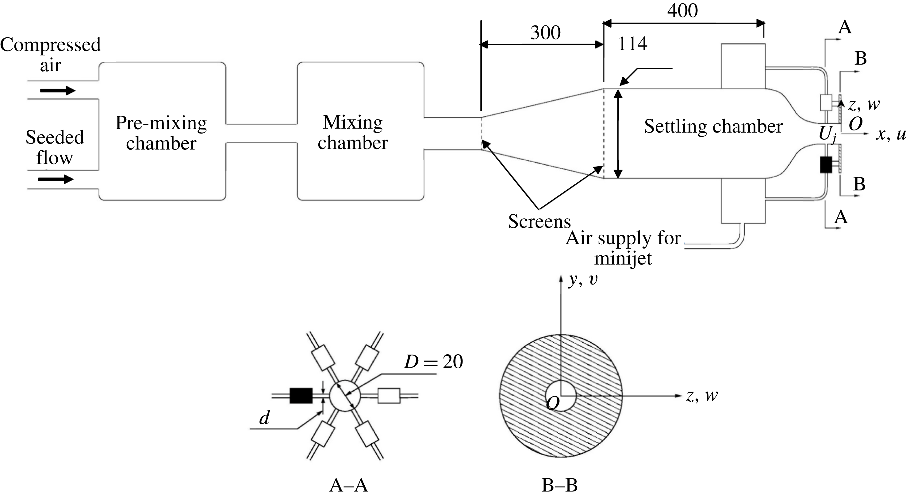
The rig consists of a main jet and a minijet assembly (figure 1). The compressed air for the main or primary jet and minijet comes from three air tanks connected in series, with a total storage capacity of
 $8~\text{m}^{3}$
and a pressure of 12 MPa, which is sufficient for 3 h in running time. The air supply to the main jet and the minijet is controlled by separate valves. The compressed air is mixed with seeding particles in the pre-mixing and mixing chamber in the case of PIV or flow visualization measurements and then enters a plenum chamber, consisting of a 300 mm long diffuser of
 $15^{\circ }$
in half-angle and a 400 mm long cylindrical settling chamber with an inner diameter of 114 mm. The flow goes through two wire-mesh screens before entering into the smooth contraction nozzle. The profile of the nozzle contraction is identical to that used in Yang & Zhou (Reference Yang and Zhou2016). The contraction is extended with a 47 mm long smooth tube, whose inner diameter is the same as the nozzle exit diameter
 $D$
(
 $=20$
mm).
Schematic of experimental rig, minijet assembly and the definition of the coordinate system.

The main jet nozzle is drilled with six holes of diameter
 $d$
, separated azimuthally by
 $60^{\circ }$
and located 17 mm upstream of the main jet exit. Three nozzles,
 $d=0.5$
, 0.8 and 1.0 mm, respectively, are made and exchangeable. Each hole is connected via a short plastic hose to an electromagnetic valve (Koganei K2-100SF-09-LL) with its maximum frequency of 1 kHz, which is used to generate unsteady minijet. The 6 electromagnetic valves are controlled independently. In this study, only one single minijet is used, which is shaded in figure 1. The valve is driven by a square-wave voltage signal of 0–5 V from the output board of a NI system and its
 $\unicode[STIX]{x1D6FC}$
may vary from 0.1 to 1.0. The square wave excitation is more effective than sinusoidal forcing (M’Closkey et al.
Reference M’Closkey, King, Cortelezzi and Karagozian2002). The
 $f_{e}$
and
 $\unicode[STIX]{x1D6FC}$
of the minijet can be adjusted by changing the frequency and duty cycle of the square-wave signal. The frequency range that can be achieved is 0–1 kHz. Mass flow rates of both main jet and minijet are adjustable independently via two separate mass flow meters, whose measurement uncertainty is no more than
 $\pm 1\,\%$
.
The coordinate system (
 $x$
,
 $y$
,
 $z$
) and its origin
 $O$
are defined in figure 1. Measurements were conducted in the minijet injection (
 $x$
–
 $z$
) plane, the orthogonal or non-injection (
 $x$
–
 $y$
) plane and at a number of cross-sectional planes (
 $y$
–
 $z$
) of the main jet. The instantaneous velocities are denoted by
 $U$
,
 $V$
and
 $W$
along
 $x$
,
 $y$
and
 $z$
, respectively, and their fluctuating components are given by
 $u$
,
 $v$
and
 $w$
, respectively.
2.2 Flow measurements and data processing
 $U$
is measured using a single tungsten wire of
 $5~\unicode[STIX]{x03BC}\text{m}$
in diameter, operated on a constant temperature circuit (Dantec Streamline) at an over-heat ratio of 1.8. The signal from the wire is offset, filtered at a cutoff frequency of 3 kHz, amplified and then digitized using a 12-bit A/D board at a sampling frequency of 6 kHz. The record duration is 80 s, which ensures that
 $u_{rms}$
is converged to within 1 % uncertainty, where subscript rms denotes the root mean square value. The hot-wire probe is mounted on a computer-controlled three-dimensional traversing mechanism, whose streamwise and transverse resolutions are 0.01 mm. The hot-wire signal is calibrated based on the streamwise mean velocity measured using a standard Pitot static tube with an outer diameter 2.2 mm, connected to an electronic micro manometer (Furness FCO510) and placed, side by side with the hot-wire, parallel to the flow near the centre of the nozzle exit. The Pitot static probe may read a lower value in an open jet of limited diameter as compared to an infinite stream, due to flow acceleration. The present blockage ratio, i.e. the ratio of the probe tip area to the nozzle exit area, is 1.2 %, smaller than the threshold of 5 %, exceeding which the blockage may incur a considerable effect on pressure and hence flow velocity measurements (Chue Reference Chue1975).
Flow visualization and particle imaging velocimetry (PIV) measurements are performed using a time-resolved Dantec standard PIV2100 in the injection and non-injection planes and also at various cross-sectional planes of the main jet. A TSI oil droplet generator (TSI 9307-6) is used to generate fog for seeding the flow. The seeding particles have a diameter of approximately
 $1~\unicode[STIX]{x03BC}\text{m}$
and are thus adequate for tracking turbulent or high-speed gas flows (Melling Reference Melling1997). The seeding particles, injected into the upstream mixing chamber, are homogeneously distributed in the main jet. Flow illumination is provided by a laser sheet of 1 mm thick generated from two standard pulsed laser sources (Beam Tech 500-10) with 532 nm wavelength and a maximum energy output of 30 mJ per pulse. The flow images are captured at a framing rate of 540 images per second using one HiSense MkII CCD camera (double frames,
 $2048\times 2048$
pixels). The Dynamic Studio v3.41 is used to synchronize flow illumination and image capturing during measurements.
In flow visualization and velocity measurements in the
 $x$
–
 $z$
and
 $x$
–
 $y$
planes, the captured image covers an area of
 $x^{\ast }=0$
–10 and
 $y^{\ast }$
or
 $z^{\ast }=-5\sim +5$
. The longitudinal and lateral image magnifications are identical,
 $0.09~\text{mm}~\text{pixel}^{-1}$
. The time interval between two consecutive laser pulses is chosen as
 $75\,\unicode[STIX]{x03BC}\text{s}$
, during which a particle could travel only 0.05 mm (4 pixels or
 $0.003D$
). In post-processing, a built-in adaptive correlation function of the Flow Map Processor (PIV 2001 type) is used with an interrogation window of
 $32\times 32$
pixels and a 75 % overlap along both directions, thus producing
 $253\times 253$
velocity vectors. The total number of images captured is 1500 pairs. It has been confirmed that the centreline mean velocity distribution calculated from snapshots of the flow field collapses already very well with the hot-wire data.
In the measurements of the flow in the
 $y$
–
 $z$
plane, the laser sheet thickness is set at approximately 3 mm, following Huang, Zhou & Zhou (Reference Huang, Zhou and Zhou2006). Similarly to Yang & Zhou (Reference Yang and Zhou2016), the camera is placed at
 $50D$
downstream from the light sheet so that the interference of the camera on the measurement is negligibly small. The image magnification is
 $0.09~\text{mm}~\text{pixel}^{-1}$
so that not only the flow field of interest is adequately covered but also the image resolution is maximized. As the axial velocity component is much larger than the two transverse components, the seeding particles could cross the 3 mm thick light sheet if the time interval between two consecutive images is large, thus causing poor correlation (Huang, Dabiri & Gharib Reference Huang, Dabiri and Gharib1997; Pattenden, Turnock & Zhang Reference Pattenden, Turnock and Zhang2005). Thus, the time interval for the present case is chosen to be
 $25~\unicode[STIX]{x03BC}\text{s}$
, which is found to yield satisfactory results. The number of velocity vectors is the same as that in the (
 $x$
–
 $y$
) and (
 $x$
–
 $z$
) planes. The total number of flow images captured is again 1500 pairs for each set of PIV data.
Experiments were conducted for a jet Reynolds number
 $Re\equiv \bar{U}_{j}D/\unicode[STIX]{x1D708}$
of 8000, where
 $\unicode[STIX]{x1D708}$
is the kinematic viscosity of air. Following Zhou et al. (Reference Zhou, Du, Mi and Wang2012) and Yang & Zhou (Reference Yang and Zhou2016),
 $K=(\bar{U}_{j}-\bar{U}_{5D})/\bar{U}_{j}$
is used to evaluate the jet entrainment rate, where
 $\bar{U}_{5D}$
denotes the jet centreline mean velocity at
 $x^{\ast }=5$
. The choice of
 $K$
is based on the following considerations. Firstly, it has been demonstrated in Zhou et al. (Reference Zhou, Du, Mi and Wang2012) that thus defined
 $K$
is correlated approximately linearly with an equivalent jet half-width
 $R_{eq}=[R_{H}R_{V}]^{1/2}$
, where
 $R_{H}$
and
 $R_{V}$
are the jet half-widths in two orthogonal planes, that is,
 $K$
is directly connected to the entrainment rate of the manipulated jet. Secondly, as documented by Fan et al. (Reference Fan, Wu, Yang, Li and Zhou2017), the difference
 $\unicode[STIX]{x0394}K$
between the
 $K$
values with and without control reaches a maximum at
 $x^{\ast }\approx 5$
(their figure 7), that is, the
 $K$
estimated based on the streamwise velocity measured at
 $x^{\ast }=5$
is most sensitive to the change in the control parameters. Thirdly, the variation in
 $K$
is almost linear from
 $x^{\ast }=0$
to
 $x^{\ast }\approx 7$
under control (figure 7, Fan et al.
Reference Fan, Wu, Yang, Li and Zhou2017), that is, a single value of
 $K$
may be used to describe reasonably well the jet decay rate in the near field under control. This is as Breidenthal et al. (Reference Breidenthal, Tong, Wong, Hamerquist and Landry1985) did, who used an aspirating probe to measure the concentration fluctuation
 $c$
of two mixing streams (a rectangular duct flow and a transverse jet) and reported that the decay rate of the root mean square value
 $c_{rms}$
of the concentration fluctuation was approximately linearly connected to the momentum ratio (
 $J$
) of the transverse jet to the rectangular duct flow. This linear relationship persisted over
 $1<x^{\ast }<10$
(see their figure 5). Therefore, they used a single decay rate of
 $c_{rms}$
, measured at
 $x^{\ast }=8.9$
, to characterize the mixing of the two streams and suggested that this decay rate provided a measure for the mixing efficacy of turbulence. So does
 $K$
in the context of the present work.
3 Initial conditions of flow under minijet injection
In the absence of any perturbation,
 $\overline{U}^{\ast }$
measured at
 $x^{\ast }=0.05$
exhibits a ‘top-hat’ profile (not shown) and the corresponding
 $u_{rms}^{\ast }=u_{rms}/\bar{U}_{j}$
is 0.3 %. The power spectral density functions
 $E_{u}$
of
 $u$
measured on the centreline over
 $x^{\ast }=2$
–6 exhibit a pronounced peak at
 $f_{0}=135$
Hz, suggesting the occurrence of preferred-mode structures. The figure that shows the preferred mode was presented in Yang & Zhou (Reference Yang and Zhou2016), and is thus not included in this article. The corresponding Strouhal number
 $St$
(
 $\equiv f_{0}D/\bar{U}_{j}$
) is 0.45, falling in the expected range of 0.24–0.64 for a natural jet (e.g. Crow & Champagne Reference Crow and Champagne1971; Gutmark & Ho Reference Gutmark and Ho1983).
It is important to document how the unsteady minijet changes the initial conditions of the main jet, which is crucial for understanding the flow physics behind jet control results. Following Zhou et al. (Reference Zhou, Du, Mi and Wang2012), we placed a single hot-wire upstream of the main jet exit at
 $x^{\ast }=-0.85$
(
 $y^{\ast }=0$
and
 $z^{\ast }=-0.35$
), where the minijet is excited at
 $\unicode[STIX]{x1D6FC}=0.1$
, 0.4 and 0.7 (
 $C_{m}=0.5\,\%$
,
 $f_{e}/f_{0}=0.5$
). The hot-wire is oriented normally to both minijet and main jet axes, thus capturing the
 $W$
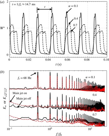
signal (figure 2
a) in the absence of the main jet or both
 $U$
and
 $W$
in the presence of the main jet (
 $\bar{U}_{j}=6~\text{m}~\text{s}^{-1}$
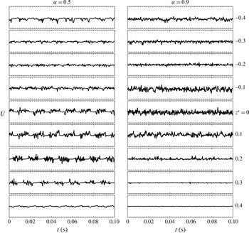
). In the absence of the main jet, the
 $W^{\ast }$
signal (figure 2
a) exhibits very distinct behaviours as
 $\unicode[STIX]{x1D6FC}$
varies, where
 $W^{\ast }=0$
and significantly above 0 correspond to the off- and on-states of the minijet, respectively. Given
 $C_{m}=0.5\,\%$
and
 $f_{e}/f_{0}=0.5$
,
 $W^{\ast }$
displays sharp peaks in the on-state, which are periodic and clearly separated for
 $\unicode[STIX]{x1D6FC}=0.1$
. However, the peaks appear less pronounced at
 $\unicode[STIX]{x1D6FC}=0.4$
and 0.7; furthermore, the on-states are not so neatly separated at
 $\unicode[STIX]{x1D6FC}=0.7$
. It seems that for
 $\unicode[STIX]{x1D6FC}\geqslant 0.7$
the off-state is temporally very limited in duration, compared to the on-state, and the excitation may actually behave closely like a quasi-steady control jet. The more pronounced peak in
 $W^{\ast }$
for
 $\unicode[STIX]{x1D6FC}=0.1$
than for
 $\unicode[STIX]{x1D6FC}=0.4$
or 0.9 implies a higher penetration depth at smaller
 $\unicode[STIX]{x1D6FC}$
, as reported by Johari et al. (Reference Johari, Pacheco-Tougas and Hermanson1999) for the pulsed jet in cross-flow. It is worth commenting that the actual duty cycle experienced in excitation may be slightly larger than the input duty cycle, as specified by an NI board, due to the fact that, even after closing the valve, there may be some fluid flowing through the tube that connects the valve and nozzle (Sailor, Rohli & Fu Reference Sailor, Rohli and Fu1999; M’Closkey et al.
Reference M’Closkey, King, Cortelezzi and Karagozian2002). In fact, the waveform observed at the output of the minijet is not really square although a great effort has been made to reduce the connection tube length between the valve and injection point to the minimum, confirming that the output or actual duty cycle may not exactly equal the input duty cycle. Apparently, the penetration depth depends on both
 $C_{m}$
and
 $\unicode[STIX]{x1D6FC}$
.
(a) Time histories measured when the main jet is not operated. (b) Power spectral density functions of streamwise fluctuating velocity
 $w$
in the absence of the main jet or
 $\sqrt{u^{2}+w^{2}}$
in the presence of the main jet, measured at
 $(x^{\ast },y^{\ast },z^{\ast })=(-0.85,0,-0.35)$
for
 $C_{m}=0.5\,\%$
,
 $f_{e}/f_{0}=0.5$
and
 $d/D=1/20$
.

 $E_{w}$
or
 $E_{\sqrt{u^{2}+w^{2}}}$
is qualitatively the same with or without the main jet operated, displaying pronounced peaks at
 $f_{e}/f_{0}$
and its harmonics (figure 2
b) in both cases. The peaks at harmonics are due to the resonance in the nozzle (Zhou et al.
Reference Zhou, Du, Mi and Wang2012), which was referred to as the parametric resonance by Huang & Hsiao (Reference Huang and Hsiao1999). Evidently, the unsteady injection produces the periodic structures in the flow before its issue from the nozzle exit. Note from figure 2 that varying
 $\unicode[STIX]{x1D6FC}$
does not affect the predominant frequencies in the spectra.
The exit velocity profile of the minijet may have an influence on the flow structure development as the parabolic profile produces a deeper penetration in the main jet than the top-hat (New, Lim & Luo Reference New, Lim and Luo2006). To envisage this, hot-wire measurements were carried out at pre-determined minijet flow rate in the absence of the main jet at a sampling frequency of 6 kHz for 100 s. The hot-wire was located approximately at the minijet exit (
 $y^{\ast }=0$
,
 $z^{\ast }=-0.475$
) and traversed, at an increment of 0.1 mm, across the minijet along the
 $x^{\ast }$
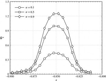
direction. Figure 3 shows the measured velocity profile of the minijet for
 $\unicode[STIX]{x1D6FC}=0.1$
, 0.5 and 0.9. A parabolic velocity profile is seen for
 $\unicode[STIX]{x1D6FC}=0.1$
, 0.5 and 0.9. The thick shear layer of the parabolic velocity profile may cause a delay in the formation of the leading-edge and lee-side vortices, compared with the thin shear layer case associated with the top-hat velocity profile (New et al.
Reference New, Lim and Luo2006).
Time-averaged velocity profiles of the minijet measured at
 $(y^{\ast },z^{\ast })=(0,-0.475)$
for
 $C_{m}=1.0\,\%$
,
 $f_{e}/f_{0}=0.5$
and
 $d/D=1/20$
in the absence of the main jet.

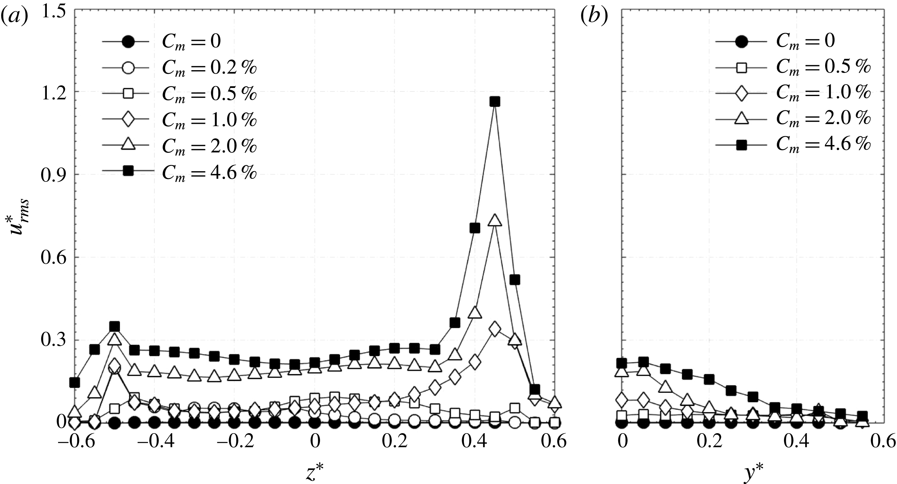
The minijet-produced structures (Yang & Zhou Reference Yang and Zhou2016) and their interaction with the main jet play a crucial role in the overall jet development. To understand the initial disturbance caused by the minijet injection on the main jet, figure 4 presents the radial distributions of
 $u_{rms}^{\ast }$
at
 $x^{\ast }=0.05$
along the injection and orthogonal non-injection directions. Note that
 $u_{rms}^{\ast }$
in the orthogonal non-injection plane is presented only for
 $y^{\ast }>0$
, assuming a reasonably symmetric distribution of
 $u_{rms}^{\ast }$
along the
 $y$
direction. As a reference, the unexcited jet (
 $C_{m}=0\,\%$
) is also shown in figure 4. There is a great change in
 $u_{rms}^{\ast }$
along both the
 $z$
and
 $y$
directions under excitation, depending on
 $C_{m}$
. At
 $C_{m}=0.20\,\%$
, the
 $u_{rms}^{\ast }$
is essentially unchanged for
 $z^{\ast }>0.15$
(figure 4
a), suggesting that the velocity disturbance produced by unsteady minijet injection is limited, leaving the shear layer at
 $z^{\ast }\approx 0.4$
–0.5 undisturbed. With
 $C_{m}$
increasing to 0.5 %, the
 $u_{rms}^{\ast }$
displays an increase for
 $z^{\ast }>0$
, indicating that the minijet has penetrated through the main jet centre and perhaps the nozzle wall feels the disturbance of the minijet, as suggested by the tiny increase in
 $u_{rms}^{\ast }$
at
 $z^{\ast }=0.5$
(figure 4
a). At
 $C_{m}=1.0\,\%$
, the
 $u_{rms}^{\ast }$
increases significantly over
 $0<z^{\ast }<0.45$
, an indication that the shear layer on the opposite side to the minijet starts to be disturbed by the injection. There is also an appreciable increase in
 $u_{rms}^{\ast }$
along the
 $y$
direction (figure 4
b). Up to this stage, the flow at the nozzle exit remains to be laminar, as is evident in the hot-wire measured
 $U$
signals along both
 $y$
and
 $z$
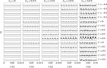
directions (figure 5). Note that the minijet, issuing from
 $z^{\ast }=-0.5$
, injects along the
 $z$
direction. The fluctuations in figure 5 apparently originate from the minijet injection into the main jet. There is no appreciable fluctuation in
 $U$
along the
 $y$
direction. At
 $C_{m}=2.0\,\%$
, the
 $u_{rms}^{\ast }$
rises very significantly over
 $-0.6<z^{\ast }<0.6$
(figure 4
a). So does
 $u_{rms}^{\ast }$
around the centre along the
 $y$
-direction. This is a sign that the minijet flow impinges upon the opposite wall of the main jet nozzle at
 $z^{\ast }=0.5$
. Nevertheless, the flow remains to be laminar or at most starts the transition, as reflected by the
 $U$
signals (figure 5). At
 $C_{m}=4.6\,\%$
,
 $u_{rms}^{\ast }$
rises sharply about
 $z^{\ast }=0.5$
along the
 $z$
-direction and meanwhile grows almost across the main jet along the
 $y$
direction. The strong minijet impingement upon the wall now starts to produce turbulence; the
 $U$
signals (figure 5) captured along both the
 $y$
and
 $z$
directions all display random fluctuations. It seems plausible that the maximum penetration depth of the minijet occurs at
 $C_{m}=2.0\,\%$
. Increasing
 $C_{m}$
to 4.6 %, the maximum penetration remains the same as that at
 $C_{m}=2.0\,\%$
; however, the substantial rise in
 $u_{rms}^{\ast }$
and the randomly fluctuating
 $U$
signals over
 $-0.6<z^{\ast }<0.6$
and
 $0<y^{\ast }<0.4$
(figures 4 and 5) suggest a fully turbulent jet right from the nozzle exit.
Radial distributions of
 $u_{rms}^{\ast }=u_{rms}/\bar{U}_{j}$
measured at
 $x^{\ast }=0.05$
(
 $f_{e}/f_{0}=0.5$
,
 $\unicode[STIX]{x1D6FC}=0.1$
,
 $d/D=1/20$
): (a) in the
 $x$
–
 $z$
or injection plane, (b) in the
 $x$
–
 $y$
or non-injection plane.

Typical signals of instantaneous streamwise
 $U$
measured along the
 $y^{\ast }$
and
 $z^{\ast }$
direction at
 $x^{\ast }=0.05$
(
 $f_{e}/f_{0}=0.5$
,
 $\unicode[STIX]{x1D6FC}=0.1$
,
 $d/D=1/20$
). The same scale is applied for all signals.

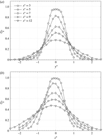
The normalized mean velocity profiles in two orthogonal planes are illustrated in figure 6 for the perturbed jet at
 $C_{m}=1.0\,\%$
,
 $f_{e}/f_{0}=0.5$
,
 $\unicode[STIX]{x1D6FC}=0.1$
and
 $d/D=1/20$
, which exhibit a reasonable symmetry about the jet centre (
 $y^{\ast }=0$
or
 $z^{\ast }=0$
) for the
 $x^{\ast }$
range examined. There is a slight deviation in the location of the maximum velocity from the geometric centre
 $z^{\ast }=0$
, as observed by Yang et al. (Reference Yang, Zhou, So and Liu2016). This is primarily a result of the asymmetric injection. The difference between the maximum velocity and the velocity at
 $z^{\ast }=0$
is in general very small, causing an error of no more than 1 % in
 $K$
. This difference becomes appreciable only for a quasi-steady control (
 $\unicode[STIX]{x1D6FC}\geqslant 0.9$
) at
 $C_{m}>3.5\,\%$
when the jet column deflects away from the geometric axis, which may be referred to as thrust vectoring. As a consequence, there is an artificial increase in
 $K$
, which will be further discussed in § 5.
Normalized streamwise mean velocities measured along the
 $y$
and
 $z$
axes at different axial locations for
 $C_{m}=1.0\,\%$
,
 $f_{e}/f_{0}=0.5$
,
 $\unicode[STIX]{x1D6FC}=0.1$
and
 $d/D=1/20$
.

4 Parametric study of jet manipulation
In this section, we document the dependence of
 $K$
on
 $f_{e}/f_{0}$
,
 $C_{m},\unicode[STIX]{x1D6FC}$
and
 $d/D$
under the minijet excitation.
4.1 Excitation frequency ratio effect
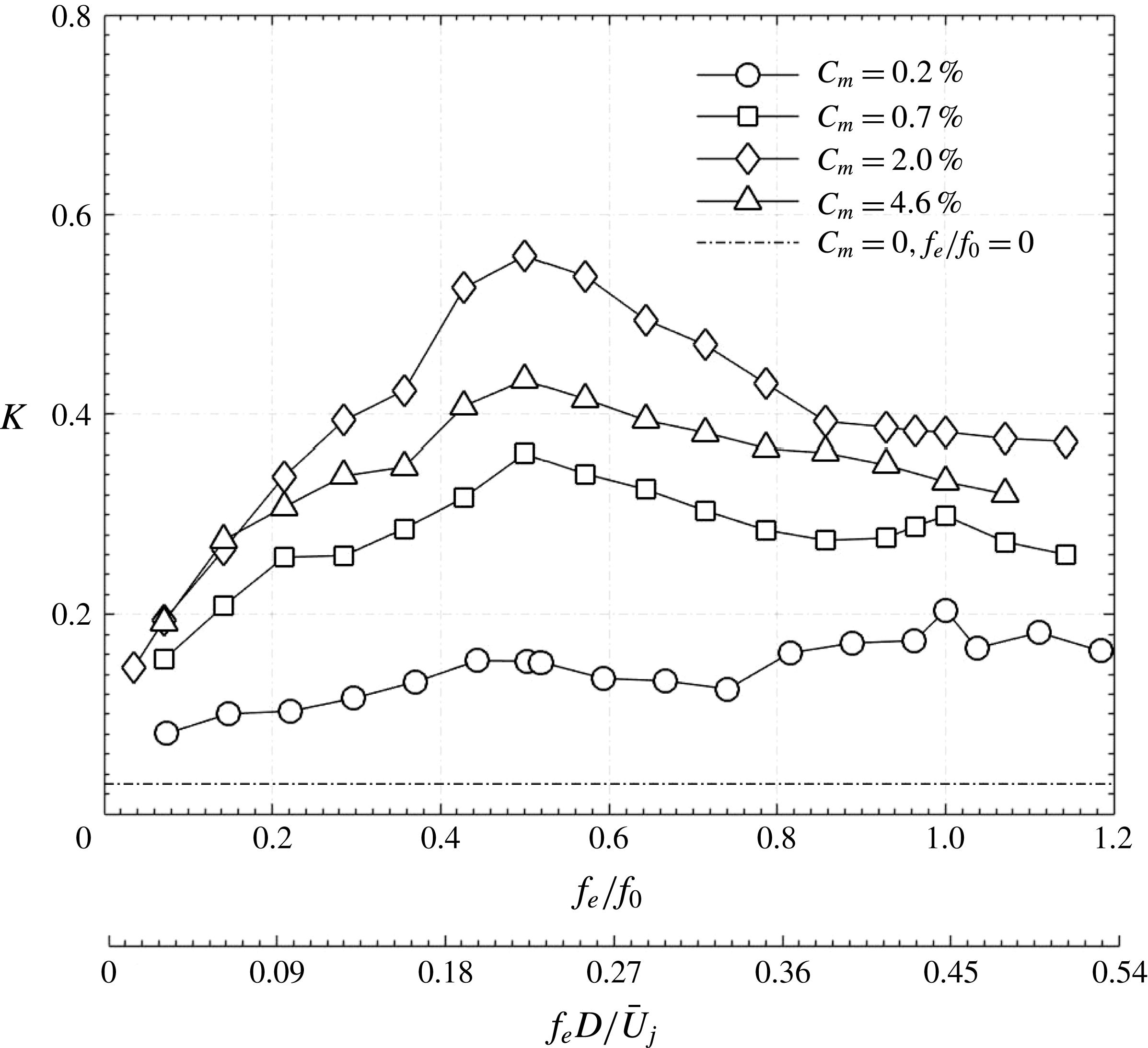
Figure 7 presents the dependence of
 $K$
on
 $f_{e}/f_{0}$
for different
 $C_{m}$
at
 $\unicode[STIX]{x1D6FC}=0.1$
. The
 $K$
of the manipulated jet exceeds greatly that (0.03) of the natural jet over the entire range of
 $f_{e}/f_{0}$
, suggesting an effective manipulation. Its value exhibits a dependence on
 $f_{e}/f_{0}$
, and may show its peak at
 $f_{e}/f_{0}=0.5$
(
 $f_{e}^{\ast }=f_{e}D/\bar{U}_{j}=0.23$
) or at
 $f_{e}/f_{0}=1.0$
(
 $f_{e}^{\ast }=0.45$
). The latter is very minor and occurs only for small
 $C_{m}$
, i.e. 0.20 % and 0.70 %. The maximum
 $K$
takes place at
 $f_{e}/f_{0}=1.0$
for
 $C_{m}\leqslant 0.2$
but at
 $f_{e}/f_{0}=0.5$
(
 $f_{e}^{\ast }=0.23$
) for
 $C_{m}>0.2\,\%$
. Freund & Moin (Reference Freund and Moin2000) conducted a direct numerical simulation of a Mach 0.9 jet at
 $Re=3.6\times 10^{3}$
, which was excited at
 $f_{e}^{\ast }=0.2$
(the subharmonic of the preferred-mode frequency) and 0.4 (
 $C_{m}=3.5\,\%$
) using two slot jets at
 $180^{\circ }$
out of phase. They revealed that
 $f_{e}^{\ast }=0.2$
produced a higher jet spread and reduced the potential core more than
 $f_{e}^{\ast }=0.4$
, that is, their subharmonic excitation was more effective than the excitation at the preferred-mode frequency. Similarly, M’Closkey et al. (Reference M’Closkey, King, Cortelezzi and Karagozian2002) also reported that the optimal jet penetration and spread for the pulsed jet in cross-flow occurred at the subharmonic excitation of the preferred-mode structures. The effective excitation at
 $f_{e}/f_{0}=0.5$
is not surprising. Ho & Huang (Reference Ho and Huang1982) noted that the spreading rate of a mixing layer can be greatly manipulated at the subharmonic of the preferred-mode frequency, where many vortices merge together through the collective interaction which is distinct from the ordinary vortex merging. Nevertheless, the physical mechanism behind this observation has not been unveiled.
Dependence of the centreline mean velocity jet decay rate
 $K$
on the excitation frequency ratio
 $f_{e}/f_{0}$
or
 $f_{e}D/\bar{U}_{j}$
for
 $\unicode[STIX]{x1D6FC}=0.1$
and
 $d/D=1/20$
.

Insight into why the maximum
 $K$
shifts from
 $f_{e}/f_{0}=1.0$
to 0.5 for
 $C_{m}>0.2$
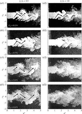
may be gained through examining typical photographs (figure 8) captured from flow visualization in the
 $x$
–
 $z$
plane of the jet, with and without manipulation. The manipulated jet depends on
 $C_{m}$
and
 $f_{e}/f_{0}$
and appears very different from the natural jet. In general, the minijet perturbation causes an early roll up of vortices in the injection plane (
 $z^{\ast }\approx -0.5$
,
 $x^{\ast }\approx 1.0$
), and the jet structure is asymmetrical or staggered in the
 $x$
–
 $z$
plane (figure 8
a1–d2) but symmetrical in the
 $x$
–
 $y$
plane (not shown). At
 $C_{m}=0.20\,\%$
and
 $f_{e}/f_{0}=0.5$
(figure 8
a1), the perturbed jet column shows an upward movement at
 $x^{\ast }\approx 1.0$
and then downward at
 $x^{\ast }\approx 1.8$
and again upward at
 $x^{\ast }\approx 2.4$
. Such an oscillation of the jet column is also reported by Freund & Moin (Reference Freund and Moin2000) and Iio et al. (Reference Iio, Hirashita, Katayama, Haneda, Ikeda and Uchiyama2013) and referred to as the flapping jet column. The flapping phenomenon occurs for
 $f_{e}/f_{0}=0.5$
and 1.0 given
 $C_{m}=0.20\,\%$
(figure 8
a1,a2) but only for
 $f_{e}/f_{0}=0.5$
at
 $C_{m}\geqslant 0.70\,\%$
(figure 8
b1,c1,d1). The subharmonic excitation (
 $f_{e}/f_{0}=0.5$
) is generally characterized by inclined ring vortices, whereas the harmonic (
 $f_{e}/f_{0}=1.0$
) is characterized by axial ring vortices. The minijet injection induces early roll up of the ring vortex near the injection point. Given an adequate penetration depth or
 $C_{m}$
, one end of an inclined ring vortex may approach a neighbouring vortex, forming zigzag-like organized structures and hence starting a pairing process at the approaching ends. This strong vortex interaction or pairing induces upward motion of fluid on one side and downward motion on the other side, generating the flapping motion. This scenario is fully consistent with the observation that the flapping jet column occurs at the subharmonic excitation and at
 $C_{m}\geqslant 0.70\,\%$
. A more detailed physical explanation and associated evidence for the occurrence of the flapping motion are given in Yang et al. (Reference Yang, Zhou, So and Liu2016).
Typical flow structures in the injection plane of the jets from flow visualization (
 $\unicode[STIX]{x1D6FC}=0.1$
,
 $d/D=1/20$
).

Typical flow structures of two sequential times in the cross-sectional planes of the perturbed jets at
 $x^{\ast }=1.0$
from flow visualization (
 $C_{m}=0.7\,\%$
,
 $\unicode[STIX]{x1D6FC}=0.1$
,
 $d/D=1/20$
).

Spectral phase
 $\unicode[STIX]{x1D719}_{U1U2}$
between two streamwise velocity signals measured in the jet at
 $x^{\ast }=2$
and
 $z^{\ast }=\pm 0.35$
excited at
 $\unicode[STIX]{x1D6FC}=0.1$
and
 $d/D=1/20$
. Dashed and continuous lines represent
 $f_{e}/f_{0}=0.5$
and 1.0, respectively.

Figure 9 shows the time sequence of cross-sectional images captured at
 $x^{\ast }=1.0$
for
 $C_{m}=0.70\,\%$
and
 $f_{e}/f_{0}=0.5$
and 1.0. The imaging rate was 540 images per second such that four and eight images were obtained for each cycle of injection at
 $f_{e}/f_{0}=1.0$
and 0.5, respectively. The time intervals,
 $\unicode[STIX]{x0394}t=t_{2}{-}t_{1}$
, are 7.4 ms for
 $f_{e}/f_{0}=0.5$
(figure 9
a) and 3.7 ms for
 $f_{e}/f_{0}=1.0$
(figure 9
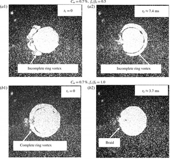
b), corresponding to one half of the injection cycle for each case (the vortex shedding period is 7.4 ms). An incomplete ring structure is observed at
 $t_{1}=0$
on the minijet injection side (
 $z^{\ast }<0$
) for
 $f_{e}/f_{0}=0.5$
(figure 9
a1), indicating the early roll up of vortical structures, but occurs largely on the other side (
 $z^{\ast }>0$
) at
 $t_{2}\approx 7.4$
ms (figure 9
a2). The difference in time between the captured incomplete ring structure of
 $z^{\ast }<0$
and
 $z^{\ast }>0$
is internally consistent with the flow structure development in the
 $x$
–
 $z$
plane (figure 8
b1) where the lower shear layer (
 $z^{\ast }<0$
) starts to roll up earlier than the upper (
 $z^{\ast }>0$
). It may be inferred that the part of the ring vortex on the minijet injection side forms early, compared with that on the other side. That is, the excitation at
 $f_{e}/f_{0}=0.5$
leads to the formation of inclined ring vortices, which evolve into the staggered arrangement (figure 8
b1) and produce the main jet column flapping, as discussed by Yang et al. (Reference Yang, Zhou, So and Liu2016). On the other hand, the images in figure 9(b1,b2) show a complete ring and a full-moon-like structure, albeit with breaches about the injection point, in the braid region, respectively, at
 $f_{e}/f_{0}=1.0$
. That is, the ring vortices are not inclined and the jet column would not flap (figure 8
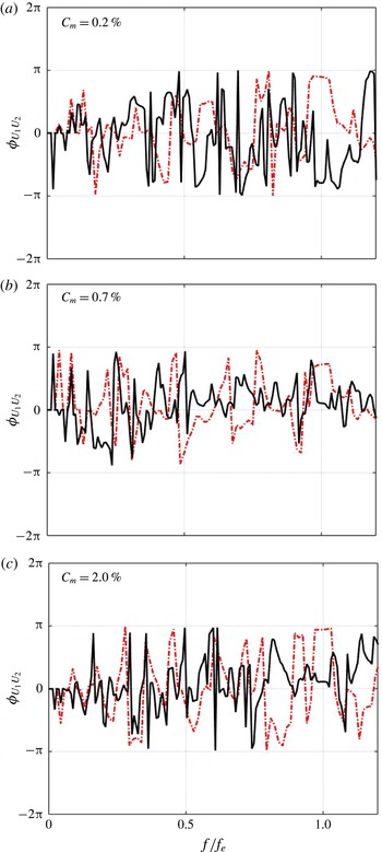
b2). The assertion is further supported by the phase spectrum
 $\unicode[STIX]{x1D6F7}_{U1U2}$
between
 $U_{1}$
and
 $U_{2}$
simultaneously measured at
 $z^{\ast }=-0.3$
and 0.3 (
 $x^{\ast }=2$
), respectively. At
 $f_{e}/f_{0}=0.5$
,
 $\unicode[STIX]{x1D6F7}_{U1U2}$
is near
 $\unicode[STIX]{x03C0}$
or
 $-\unicode[STIX]{x03C0}$
, i.e. anti-phased, displaying unmistakably a plateau about
 $f/f_{e}=1.0$
, regardless of
 $C_{m}$
, (figure 10). The result indicates unambiguously that the flow structure shown in the left column of figure 8 is indeed representative of the flow. On the other hand, at
 $f_{e}/f_{0}=1.0$
,
 $\unicode[STIX]{x1D6F7}_{U1U2}$
is near zero at
 $f/f_{e}=1.0$
for
 $C_{m}>0.20\,\%$
, suggesting the absence of the flapping motion. It is the occurrence of flapping that increases significantly the jet decay rate or
 $K$
, as shown in figure 7.
4.2 Duty cycle effect
The duty cycle
 $\unicode[STIX]{x1D6FC}$
is the fraction of time the minijet is being injected during each injection cycle. This is a very important parameter for jet manipulation using unsteady minijet. However, there has been so far no report on the influence of
 $\unicode[STIX]{x1D6FC}$
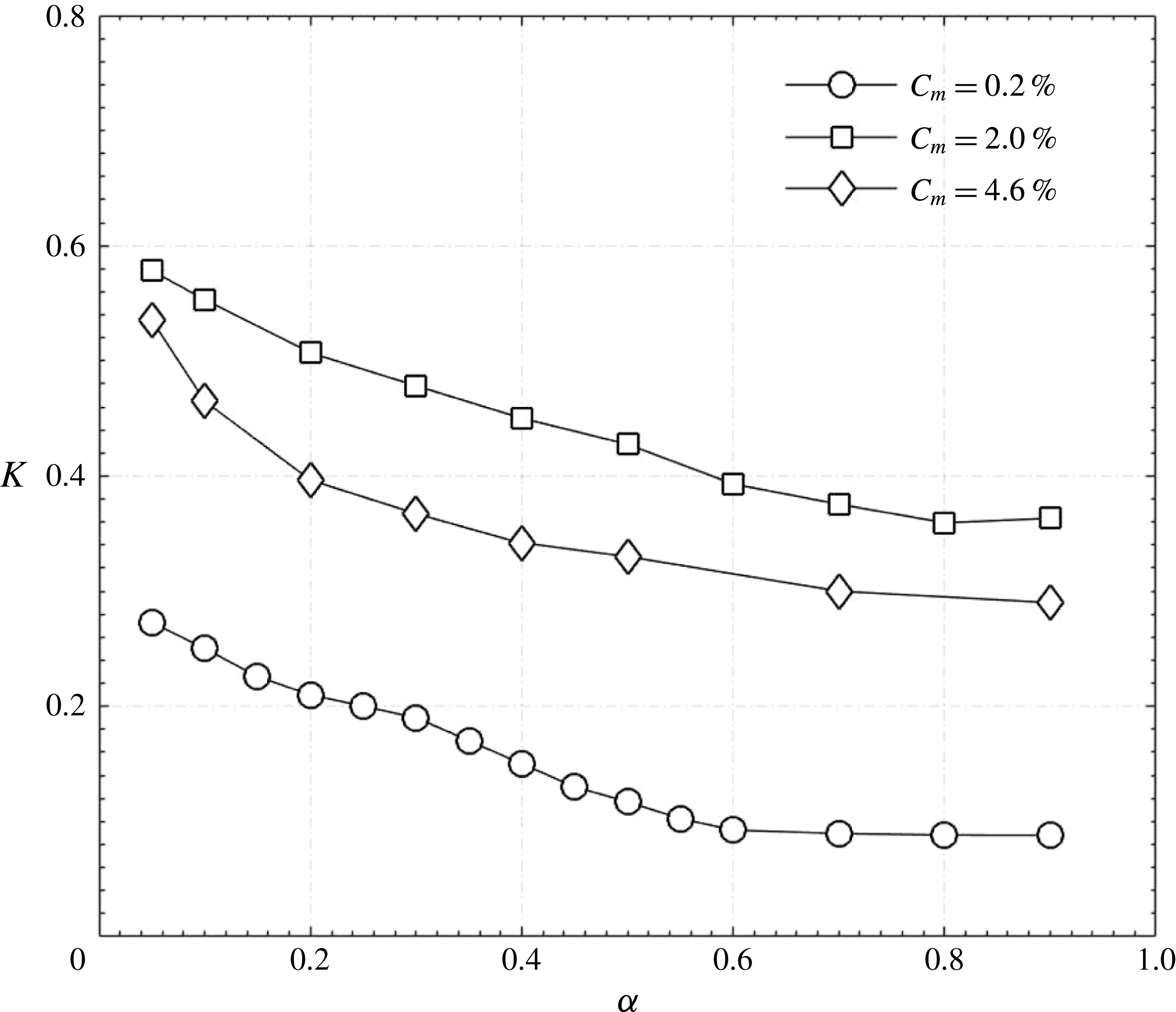
on the jet control performance. Figure 11 presents the dependence of
 $K$
on
 $\unicode[STIX]{x1D6FC}$
for three representative
 $C_{m}$
at
 $f_{e}/f_{0}=0.5$
. The
 $K$
decreases from
 $\unicode[STIX]{x1D6FC}=0.1$
to 0.9 for all
 $C_{m}$
, although varying little for
 $\unicode[STIX]{x1D6FC}\geqslant 0.7$
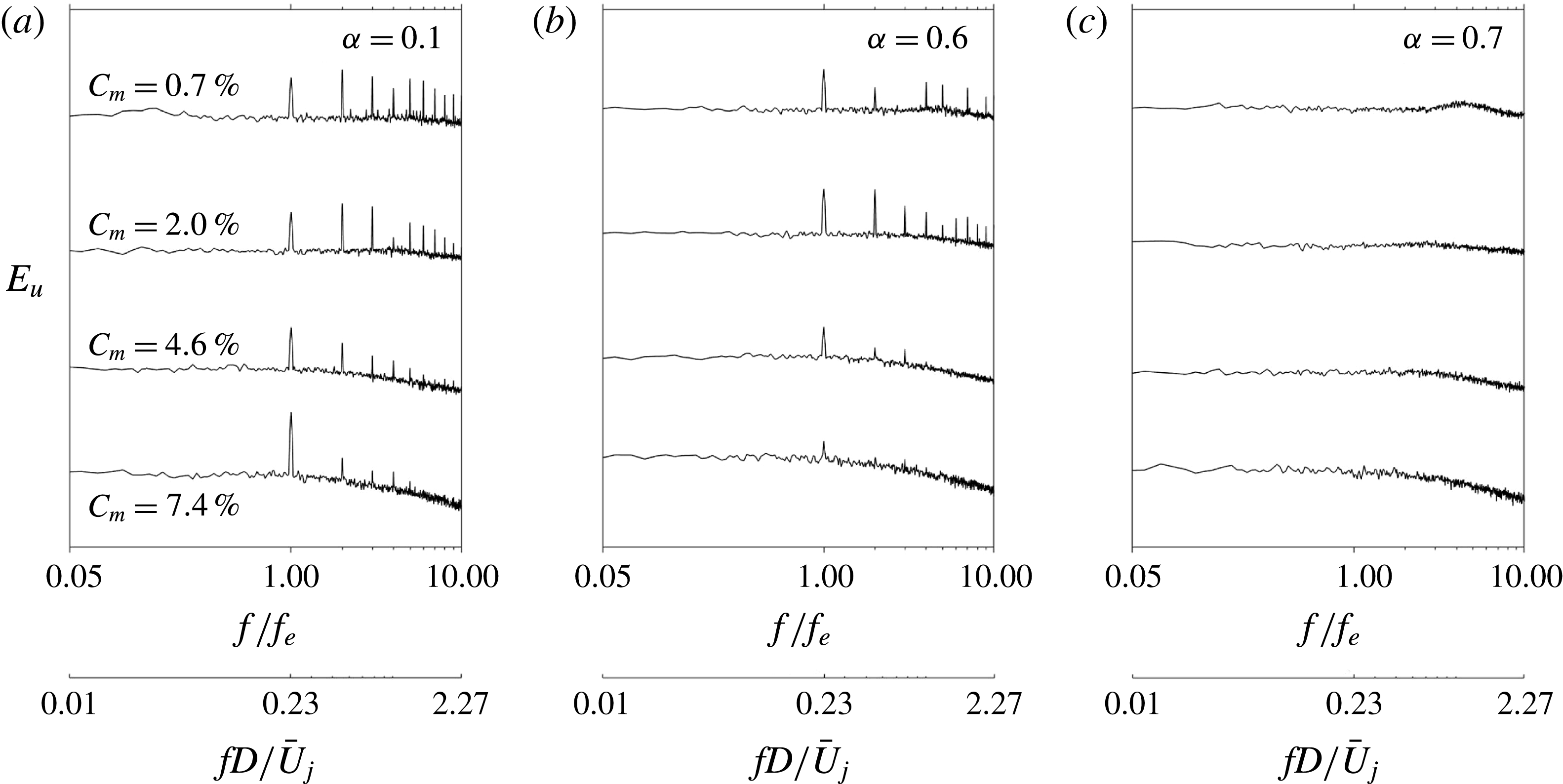
. At
 $\unicode[STIX]{x1D6FC}=0.1$
or 0.6,
 $E_{u}$
measured at
 $(x^{\ast },y^{\ast },z^{\ast })=(0.5,0,-0.35)$
exhibits pronounced peaks at
 $f/f_{e}=1.0$
(
 $f_{e}=68~\text{Hz}$
,
 $f_{e}^{\ast }=0.23$
) and its sub-harmonics (figure 12
a,b) but not at
 $\unicode[STIX]{x1D6FC}=0.7$
(figure 12
c), irrespective of
 $C_{m}$
, suggesting that the natural preferred-mode instability is not excited at the larger
 $\unicode[STIX]{x1D6FC}$
. Johari (Reference Johari2006) made a similar observation (see his figure 6) when studying the interaction of a pulsed jet in cross-flow at a large duty cycle, which they referred to as a quasi-steady blowing jet.
Dependence on
 $\unicode[STIX]{x1D6FC}$
of the jet centreline mean velocity decay rate
 $K$
(
 $f_{e}/f_{0}=0.5$
,
 $d/D=1/20$
).

Power spectral density function of streamwise fluctuating velocity
 $u$
measured at
 $x^{\ast }=0.5$
and
 $z^{\ast }=-0.35$
for the jet excited at
 $f_{e}/f_{0}=0.5$
and
 $d/D=1/20$
.

The duty cycle is connected to the penetration of the pulsed control jet (Johari et al.
Reference Johari, Pacheco-Tougas and Hermanson1999). Consider the
 $U$
signals at
 $\unicode[STIX]{x1D6FC}=0.1$
(figure 5), 0.5 and 0.9 (figure 13) along the
 $z$
direction (
 $x^{\ast }=0.05$
,
 $C_{m}=1.0\,\%$
). At
 $\unicode[STIX]{x1D6FC}=0.1$
, the periodic fluctuations of the signals, apparently originating from the minijet injection, appear from
 $z^{\ast }=-0.4$
to 0.4 and gradually increase in their magnitude as
 $z^{\ast }$
increases. At
 $\unicode[STIX]{x1D6FC}=0.5$
, the signals appear all fluctuating randomly, indicating a turbulent jet right from the nozzle exit. Note the gradual drop in the fluctuation magnitude from
 $z^{\ast }=0.2$
to 0.4, distinctly different from that at
 $\unicode[STIX]{x1D6FC}=0.1$
, suggesting a reduced penetration depth from
 $\unicode[STIX]{x1D6FC}=0.1$
to 0.5. This drop is more obvious at
 $\unicode[STIX]{x1D6FC}=0.9$
, where the velocity fluctuations are barely discernible at
 $z^{\ast }>0.3$
, that is, the penetration depth retreats further. It is worth pointing out that the decrease in the penetration depth with increasing
 $\unicode[STIX]{x1D6FC}$
is due to the fact that, given the same
 $C_{m}$
, the minijet injection velocity during the ‘on-state’ decreases with increasing
 $\unicode[STIX]{x1D6FC}$
(figure 2
a).
Typical signals of instantaneous streamwise
 $U$
measured along the
 $z^{\ast }$
direction in the plane of
 $x^{\ast }=0.05$
(
 $C_{m}=1.0\,\%$
,
 $f_{e}/f_{0}=0.5$
,
 $d/D=1/20$
). The same scale is applied for all signals.

The change in the flow structure in the
 $x$
–
 $z$
plane (injection plane) under the influence of
 $\unicode[STIX]{x1D6FC}$
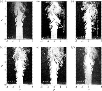
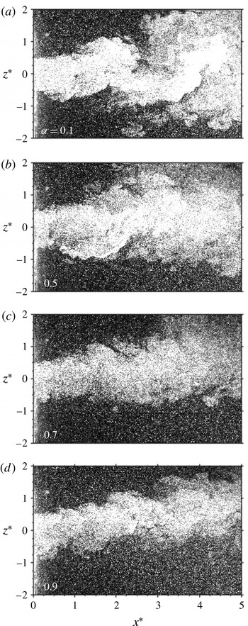
is examined in figure 14 to seek the understanding of the flow physics behind the
 $\unicode[STIX]{x1D6FC}$
effect on
 $K$
(figure 11). As a reference, the unexcited jet is shown in figure 14(a). There is a profound change in the flow structure with and without excitation. In general, the shear layer rolls up early to form vortices in the injection plane (figure 14
b–f). A large amount of ambient fluid (dark coloured) in the injection plane is entrained into the jet through the vortical structure, causing the jet to spread. The flow structure apparently flaps at
 $\unicode[STIX]{x1D6FC}=0.1$
(figure 14
b) and the flow structure appears quite similar to each other from
 $\unicode[STIX]{x1D6FC}=0.3$
to 0.9 (figure 14
b–e). Three successive vortices may be identified at
 $z^{\ast }\approx 0.5$
for
 $\unicode[STIX]{x1D6FC}\geqslant 0.3$
. The observations are consistent with the hot-wire signals. At
 $z^{\ast }=-0.4$
the signal exhibits sharp peaks for
 $\unicode[STIX]{x1D6FC}=0.1$
(figure 5), which are less sharped as
 $\unicode[STIX]{x1D6FC}$
increases. The peaks originate from the minijet injection, which induces the early roll up of the ring structures. At
 $\unicode[STIX]{x1D6FC}=0.5$
and 0.9 the time interval between two successive peaks diminishes (figure 13). The ring vortices are clearly separated at
 $\unicode[STIX]{x1D6FC}=0.1$
and the increase in
 $\unicode[STIX]{x1D6FC}$
leads to a reduced separation between the ring vortices.
Typical flow structures in the injection and non-injection planes of the jet from flow visualization (
 $C_{m}=0.2\,\%$
,
 $f_{e}/f_{0}=0.5$
,
 $d/D=1/20$
).

We may gain an insight into the physics behind the ring vortex formation by examining the time sequence (
 $\unicode[STIX]{x0394}t\approx 3.7$
ms) of cross-sectional images captured at
 $x^{\ast }=1.0$
for one cycle of injection (
 $=1/68$
s) for
 $\unicode[STIX]{x1D6FC}=0$
(unperturbed jet), 0.1, 0.5 and 0.9 (
 $C_{m}=0.20\,\%$
, figure 15). The unperturbed jet retains the circular shape of the nozzle exit (figure 15
a1–a4), showing no roll-up motion. At
 $t_{1}$
and
 $t_{2}$
(figure 15
b1–b2), an incomplete ring structure occurs in the region of
 $z^{\ast }<0$
at
 $\unicode[STIX]{x1D6FC}=0.1$
, indicating the early roll up of the vortex. But this structure cannot be captured for the next two images of the cycle (figure 15
b3–b4). The observation suggests that at
 $\unicode[STIX]{x1D6FC}=0.1$
the vortex formed during one injection is clearly separated from that during next injection, as shown in figure 14(b). At
 $\unicode[STIX]{x1D6FC}=0.5$
, an incomplete ring structure or a rupture on the circular jet column is captured for the first three images (figure 15
c1–c3) and only disappears in the last image (figure 15
c4). Clearly, an increase in
 $\unicode[STIX]{x1D6FC}$
leads to a reduced gap between the successive injections, and the vortices in figure 14(d) appear to be closely separated, especially on the injection side. At
 $\unicode[STIX]{x1D6FC}=0.9$
, the incomplete ring vortex is captured in figure 15(d1) and the rupture, progressively getting deeper, is evident for the next three images (figure 15
d2–d4), suggesting a continuous penetration. In summary, the ring vortices are clearly separated at
 $\unicode[STIX]{x1D6FC}=0.1$
and an increase in
 $\unicode[STIX]{x1D6FC}$
results in a reduced gap between perturbations at
 $\unicode[STIX]{x1D6FC}=0.5$
and even continuous perturbation and penetration at
 $\unicode[STIX]{x1D6FC}=0.9$
.
Time sequence (
 $\unicode[STIX]{x0394}t\approx 0.03$
ms) of the flow structure in the
 $y$
–
 $z$
plane (
 $x^{\ast }=1.0$
) of the jet from flow visualization (
 $C_{m}=0.2\,\%$
,
 $f_{e}/f_{0}=0.5$
,
 $d/D=1/20$
).

Johari et al. (Reference Johari, Pacheco-Tougas and Hermanson1999) and Eroglu & Breidenthal (Reference Eroglu and Breidenthal2001) suggested that the duty cycle and excitation frequency of a control jet may influence the penetration, flow structure and mass mixing characteristics in a cross-flow. Hermanson, Wahba & Johari (Reference Hermanson, Wahba and Johari1998) proposed that interaction between a jet and cross-flow is characterized by two parameters, i.e. the injection time
 $\unicode[STIX]{x1D70F}=\unicode[STIX]{x1D6FC}f_{e}$
and
 $\unicode[STIX]{x1D6FC}$
. Short and long
 $\unicode[STIX]{x1D70F}$
correspond to compact vortex rings and turbulent puff-like structures, respectively. On the other hand, the higher
 $\unicode[STIX]{x1D6FC}$
leads to more intense interaction between turbulent jet puffs and correspondingly less jet penetration. In other words, the jet in cross-flow produces distinct vortex rings with spacing and strength dictated by
 $f_{e}$
and
 $\unicode[STIX]{x1D6FC}$
(Eroglu & Breidenthal Reference Eroglu and Breidenthal2001; Sau & Mahesh Reference Sau and Mahesh2010; Coussement, Gicquel & Degrez Reference Coussement, Gicquel and Degrez2012 and Karagozian Reference Karagozian2014). For a given
 $\unicode[STIX]{x1D6FC}$
, a higher
 $f_{e}/f_{0}$
reduces the time interval and hence spatial separation between two successive injections. Naturally, there should exist optimum
 $\unicode[STIX]{x1D6FC}$
and
 $f_{e}/f_{0}$
in jet mixing enhancement. The present optimum
 $\unicode[STIX]{x1D6FC}$
and
 $f_{e}/f_{0}$
to achieve the maximum
 $K$
are 0.05 and 0.5, respectively (figures 7 and 11). Thus, under the optimal condition, the deep penetration and strong well-separated vortices are produced, leading to the flapping motion and hence mixing enhancement. At higher
 $\unicode[STIX]{x1D6FC}$
, the vortex rings excited by the successive pulses interact among themselves, thereby adversely affecting the mixing capability.
4.3 Mass flow rate ratio effect
The decay rate
 $K$
exhibits a strong dependence on
 $C_{m}$
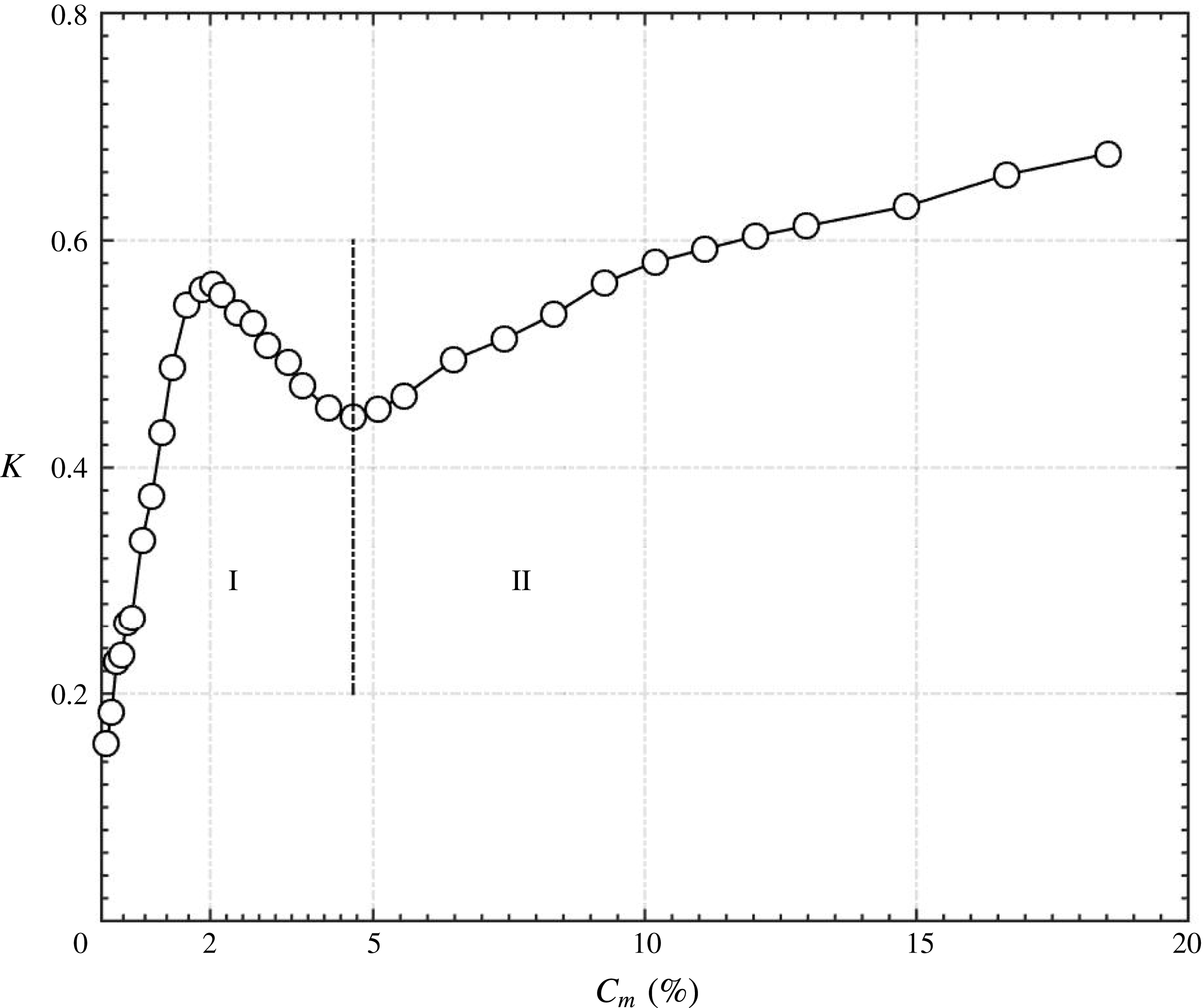
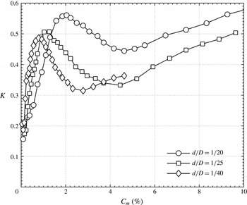
(figure 16), which can be divided into two categories based on the mechanisms. In Category I (
 $C_{m}<4.6\,\%$
),
 $K$
is highly sensitive to
 $C_{m}$
, rising rapidly from 0.16 at
 $C_{m}=0.04\,\%$
to approximately 0.56 at
 $C_{m}=2.0\,\%$
and then dropping quickly until
 $C_{m}=4.6\,\%$
. The enhanced
 $K$
results largely from the greatly modified organized motions or the generation of the flapping jet column. The maximum
 $K$
of Category I reaches 0.56, approximately 19 times that (0.03) of the natural jet and over 1.6 times that (0.34) under steady minijet injection given the same
 $C_{m}$
(
 $=$
2.0 %). This maximum occurs at the maximum penetration depth (figure 5). The drop in
 $K$
from
 $C_{m}=2.0\,\%$
until 4.6 % is a result of reduced flapping strength due to the adverse effect of turbulence generation on the organized structure development. The flapping jet is characterized by
 $\unicode[STIX]{x1D6F7}_{U1U2}=\unicode[STIX]{x03C0}$
(Yang et al.
Reference Yang, Zhou, So and Liu2016), which is found to decrease from
 $\unicode[STIX]{x03C0}$
at
 $C_{m}=2.0\,\%$
(figure 10
c) to 0.3 at
 $C_{m}=4.6\,\%$
(not shown). In Category II (
 $C_{m}\geqslant 4.6\,\%$
), the jet column flapping disappears; however,
 $K$
increases steadily, albeit much less rapidly than in Category I, and appears approaching asymptotically to a constant. The increase in
 $K$
is essentially due to the enhanced turbulence with increasing
 $C_{m}$
(Yang & Zhou Reference Yang and Zhou2016). In summary, it is a difference in the vortex dynamics that produces a great variation in
 $K$
.
Dependence on
 $C_{m}$
of the jet centreline mean velocity decay rate
 $K$
(
 $f_{e}/f_{0}=0.5$
,
 $\unicode[STIX]{x1D6FC}=0.1$
,
 $d/D=1/20$
).

It is worth examining the dependence on
 $C_{m}$
of the potential core length
 $L_{PC}^{\ast }$
, over which
 $\bar{U}^{\ast }$
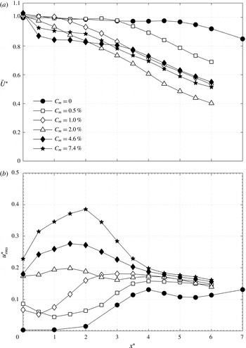
on the centreline is constant, for Categories I and II. This length is an authentic measure to quantify mixing. Shorter this length higher is the mixing enhancement due to the control (e.g. Bradbury & Khadem Reference Bradbury and Khadem1975). Figure 17(a) presents the variation of
 $\bar{U}^{\ast }$
along the jet centreline for various
 $C_{m}$
. In Category I,
 $L_{PC}^{\ast }$
is 2.5, 1.0 and 0 for
 $C_{m}=0.5\,\%$
, 1.0 % and 2.0 %, respectively, that is,
 $L_{PC}^{\ast }$
contracts for increasing
 $C_{m}$
.
 $L_{PC}^{\ast }=0$
at
 $C_{m}=2.0\,\%$
points to rapid mixing (figure 8
c1) right from the nozzle exit, corresponding to the local maximum peak in
 $K$
(figure 16). With further increase in
 $C_{m}$
,
 $L_{PC}^{\ast }$
remains at zero (figure 17
a) but the turbulence level rises continuously, which is responsible for the steady drop in
 $\bar{U}^{\ast }$
and a great enhancement in
 $u_{rms}^{\ast }$
over
 $0<x^{\ast }<3$
(figure 17
b). However, the decay of
 $\bar{U}^{\ast }$
is approximately linear over
 $3<x^{\ast }<6$
, along with a continuous drop in
 $u_{rms}^{\ast }$
. The combined effect leads to a decrease in
 $K$
from
 $C_{m}=2.0\,\%$
to 4.6 %.
(a) Streamwise mean velocity
 $\bar{U}^{\ast }$
and (b) root mean square velocity
 $u_{rms}^{\ast }$
along the jet centreline (
 $f_{e}/f_{0}=0.5$
,
 $\unicode[STIX]{x1D6FC}=0.1$
,
 $d/D=1/20$
) for various
 $C_{m}$
in Category I.

4.4 Diameter ratio effect
The
 $K$
exhibits a strong dependence on
 $d/D$
(figure 18). A number of observations can be made. Firstly, for all
 $d/D$
the dependence of
 $K$
on
 $C_{m}$
(
 $f_{e}/f_{0}=0.5$
and
 $\unicode[STIX]{x1D6FC}=0.1$
) is qualitatively the same and may be divided into two categories, i.e. a rapid rise to a local maximum
 $K$
followed by a drop (Category I) and then a monotonic growth with increasing
 $C_{m}$
(Category II). Secondly, for a given small
 $C_{m}$
(
 ${<}$
1 %) in Category I, the decay rate for
 $d/D=1/40$
is in general significantly larger than that for
 $d/D=1/25$
, and the latter exceeds that for
 $d/D=1/20$
, that is, the smaller
 $d/D$
is more efficient in enhancing mixing than the larger. This is because at a given
 $C_{m}$
the smaller
 $d/D$
is associated with a larger penetration depth due to the increased injection velocity. However, this trend may be reversed at
 $C_{m}$
exceeding 1 %. Once the penetration depth reaches the maximum, a further increase in
 $C_{m}$
will enhance the impingement strength upon the wall, thus producing turbulence and adversely influencing the development of the organized motions or jet flapping. As a consequence,
 $K$
contracts. Thirdly, the monotonic growth in
 $K$
with increasing
 $C_{m}$
in Category II is approximately linear, irrespective of
 $d/D$
, with almost the same slope. Finally, the
 $K$
for different
 $d/D$
reaches the local maximum at a different
 $C_{m}$
or the momentum in Category I. The larger
 $d/D$
corresponds to a greater
 $C_{m}$
and also a greater local maximum
 $K$
. While the maximum penetration depth might be the same for different
 $d/D$
, the corresponding momentum is higher, as a result of bigger
 $C_{m}$
, for the larger
 $d/D$
. This higher momentum should promote to a greater extent the strength of the large-scale vortices and hence the strength of jet column flapping. Consequently, the corresponding local maximum
 $K$
is larger.
Dependence on
 $d/D$
on the jet centreline mean velocity decay rate
 $K$
(
 $f_{e}/f_{0}=0.5$
,
 $\unicode[STIX]{x1D6FC}=0.1$
).

5 Empirical scaling of jet decay rate
As shown in § 4,
 $K$
depends on
 $C_{m}$
,
 $f_{e}/f_{0}$
,
 $\unicode[STIX]{x1D6FC}$
and
 $d/D$
, i.e.
 $K=g_{1}$
(
 $C_{m}$
,
 $f_{e}/f_{0}$
,
 $\unicode[STIX]{x1D6FC}$
,
 $d/D$
). In this paper,
 $g_{i}$
is a function, where
 $i=1$
, 2, 3, 4. An empirical scaling analysis is performed for the jet decay rate in order to find a scaling factor
 $\unicode[STIX]{x1D709}$
so that
 $K=g_{1}$
(
 $C_{m}$
,
 $f_{e}/f_{0}$
,
 $\unicode[STIX]{x1D6FC}$
,
 $d/D$
) may be reduced to
 $K=g_{2}$
(
 $\unicode[STIX]{x1D709}$
). Valuable insight into the flow control physics behind the influence of the minijet parameters on the flow development may be gained out of this analysis. Scaling analysis also provides the information of the control parameters on extending the laboratory experiments to the full-scale application, i.e. guiding the flow control in practical applications.
As is clear in figure 18, the dependence of
 $K$
on
 $C_{m}$
(
 $f_{e}/f_{0}=0.5$
and
 $\unicode[STIX]{x1D6FC}=0.1$
) remains unchanged qualitatively as
 $d/D$
varies. Given the same
 $C_{m}$
, the minijet velocity increases as
 $d/D$
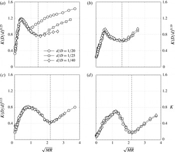
is reduced. Physically, the penetration depth of the minijet is determined by the combined effect of the minijet mass flow rate and the minijet exit velocity, that is, the momentum of the minijet plays an important role in determining the overall effectiveness in jet manipulation. After careful physical analysis of the experimental data in figure 18 along with many trial-and-error attempts, it has been found that the rescaled
 $K$
or
 $K(D/d)^{0.25}$
collapses reasonably well in Category I for various
 $d/D$
(figure 19
a) provided that the abscissa is given in terms of the momentum ratio
 $MR={\dot{m}}_{m}\bar{U}_{m}/{\dot{m}}_{j}\bar{U}_{j}$
of the minijet to main jet, where
 ${\dot{m}}$
and
 $\bar{U}$
represent the jet mass flow rate and exit velocity, respectively, and subscripts
 $m$
and
 $j$
denote minijet and main jet, respectively.
 $MR$
can be further written as
 $=({\dot{m}}_{m}/{\dot{m}}_{j})^{2}(\unicode[STIX]{x1D70C}_{j}/\unicode[STIX]{x1D70C}_{m})(A_{j}/A_{m})$
, where
 $\unicode[STIX]{x1D70C}$
and
 $A$
are the density of fluid (air) and the exit area of the minijet or nozzle exit, respectively. For incompressible flow,
 $MR=({\dot{m}}_{m}/{\dot{m}}_{j})^{2}(D/d)^{2}=C_{m}^{2}(D/d)^{2}$
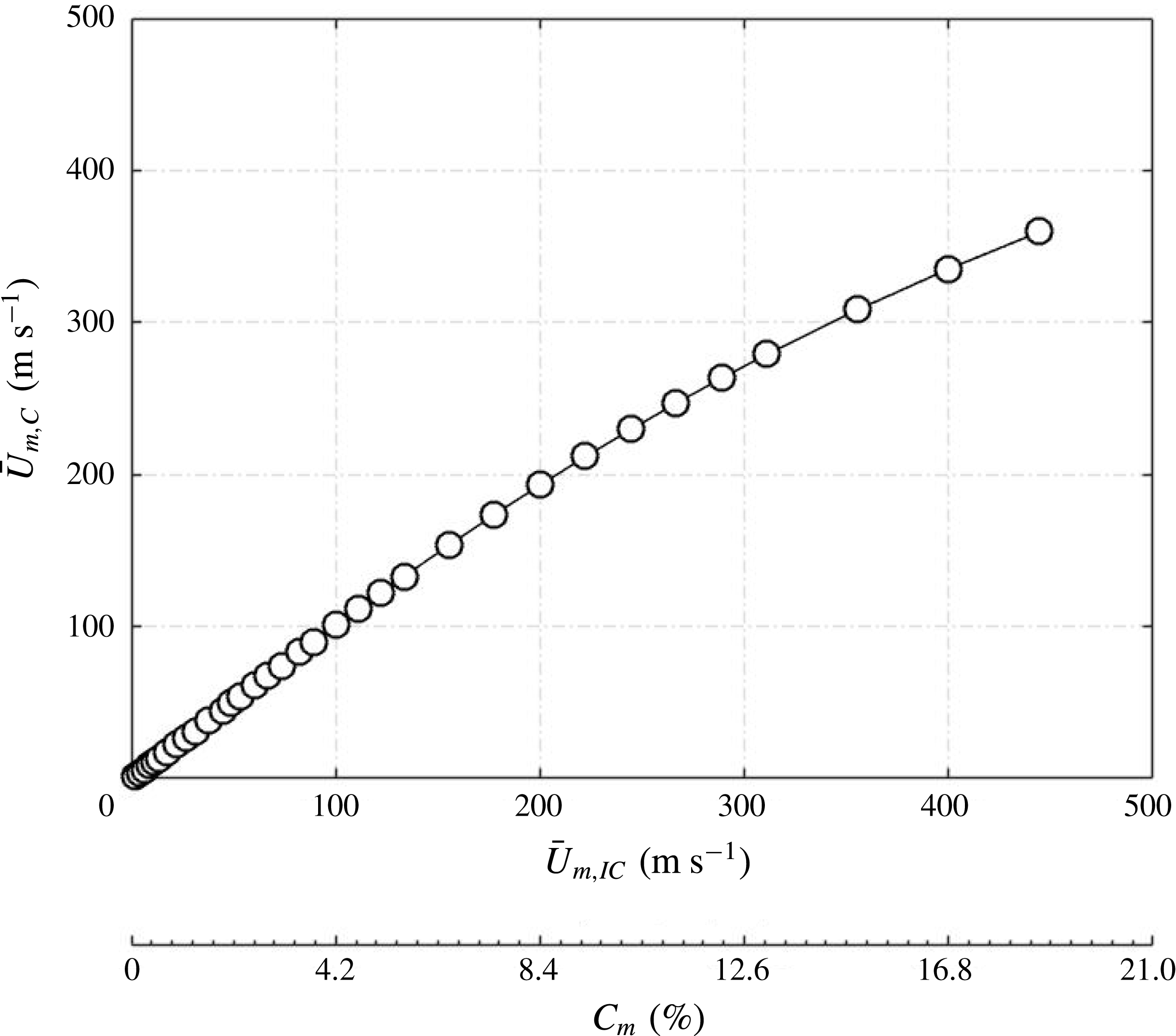
. One may question whether the incompressible assumption is valid for the minijet injection at large
 $C_{m}$
. Given
 $C_{m}<8.2\,\%$
, the error incurred in estimating the minijet velocity from the incompressible assumption is no more than 3 %. Please refer to the Appendix for the determination of errors. The result indicates that
 $\sqrt{MR}$
is the controlling scaling factor. The dependence of
 $K(D/d)^{0.25}$
on
 $\sqrt{MR}$
for
 $d/D=1/20$
does not collapse for
 $\sqrt{MR}>1.0$
with those for
 $d/D=1/25$
and
 $1/40$
. This is because the injected flow through the minijet nozzle of very small diameter (
 $d/D\leqslant 1/25$
) may have been partially choked at a large
 $C_{m}$
, thus resulting in a
 $K$
value smaller than that expected.
Dependence of the re-scaled centreline mean velocity jet decay rate on
 $\sqrt{MR}$
(
 $f_{e}/f_{0}=0.5$
,
 $\unicode[STIX]{x1D6FC}=0.1$
); (a)
 $\unicode[STIX]{x1D6FC}=0.1$
, (b) 0.3, (c) 0.5, (d) 0.9.

A similar collapse is obtained for
 $\unicode[STIX]{x1D6FC}=0.3$
, 0.5 and 0.9 (figure 19
b–d), although the measured
 $K$
is now re-scaled to
 $K(D/d)^{0.19}$
,
 $K(D/d)^{0.13}$
and
 $K(D/d)^{0.00}$
, respectively. As a matter of fact, this collapse is well observed for Category II as well as Category I since the choking phenomenon may not occur for
 $\unicode[STIX]{x1D6FC}\geqslant 0.3$
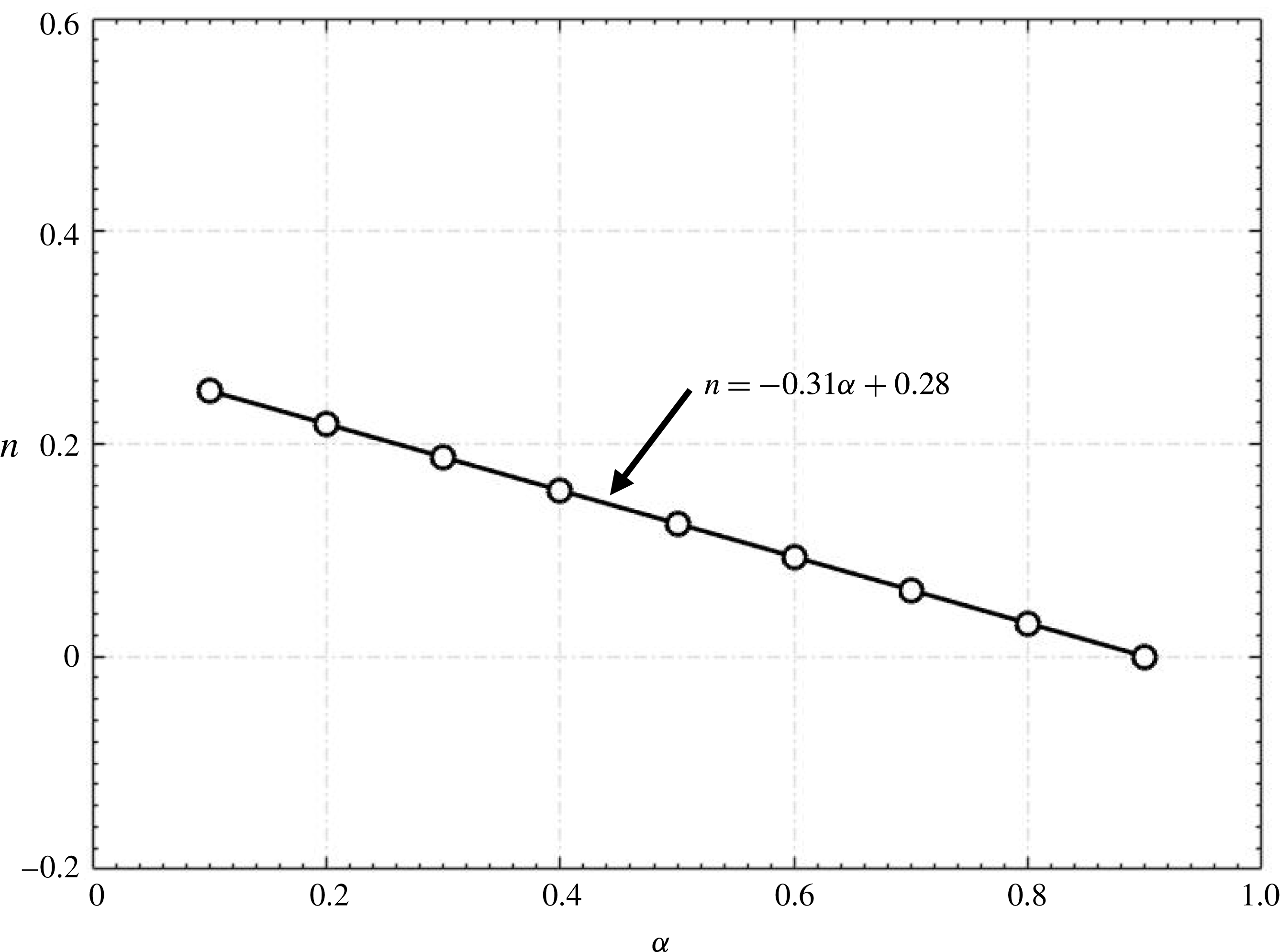
in the present experimental conditions. Apparently, the power index
 $n$
depends on
 $\unicode[STIX]{x1D6FC}$
, which are interestingly linearly correlated by
 $n=C\unicode[STIX]{x1D6FC}+0.28$
for
 $\unicode[STIX]{x1D6FC}=0.1-0.9$
, where
 $C$
is
 $-0.31$
(figure 20). As such, we may write
 $K(D/d)^{n}=g_{3}$
(
 $\sqrt{MR}$
), where
 $n=-0.31\unicode[STIX]{x1D6FC}+0.28$
. Note that
 $n<0.06$
for
 $\unicode[STIX]{x1D6FC}>0.7$
, that is,
 $n$
is approximately zero, as shown in figure 20, and the corresponding minijet injection may be referred to as the quasi-steady injection.
Variation of
 $n$
in
 $K(D/d)^{n}$
with
 $\unicode[STIX]{x1D6FC}$
.

In figures 19 and 20,
 $f_{e}/f_{0}$
is fixed at 0.5. One may wonder whether the rescaled
 $K$
or
 $K(D/d)^{n}$
would collapse over the range of
 $f_{e}/f_{0}$
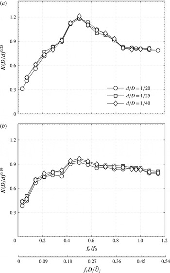
examined. Figure 21 illustrates at
 $\unicode[STIX]{x1D6FC}=0.1$
and 0.3 that
 $K(D/d)^{n}$
collapses for different
 $d/D$
, that is,
 $n$
is independent of
 $f_{e}/f_{0}$
. We will discuss in detail the physical meaning of
 $(D/d)^{n}$
later in this section.
Dependence on
 $f_{e}/f_{0}$
or
 $f_{e}D/\bar{U}_{j}$
of the rescaled centreline mean velocity jet decay rate. (a)
 $\sqrt{MR}=0.4$
,
 $\unicode[STIX]{x1D6FC}=0.1$
; (b)
 $\sqrt{MR}=0.5$
,
 $\unicode[STIX]{x1D6FC}=0.3$
.

A careful analysis along with numerous trial-and-error attempts at least-squares fitting of the data in Category I indicates that the relationship between
 $K(D/d)^{n}$
,
 $\sqrt{MR}$
and
 $\unicode[STIX]{x1D6FC}$
may be written as
 $$\begin{eqnarray}\displaystyle K\left(\frac{D}{d}\right)^{n}=g_{4}\left(\frac{\sqrt{MR}}{\unicode[STIX]{x1D6FC}}\right), & & \displaystyle\end{eqnarray}$$
where
 $\sqrt{MR}/\unicode[STIX]{x1D6FC}=(C_{m}/\unicode[STIX]{x1D6FC})(D/d)$
is physically the momentum per pulse of injection. Apparently, for a given minijet diameter and
 $C_{m,}$
an increase in
 $\unicode[STIX]{x1D6FC}$
results in a reduced momentum per pulse of injection and subsequently a reduced penetration depth into the main jet. Consequently,
 $K$
decreases, as illustrated in figure 11. On the other hand, for given
 $C_{m}$
and
 $\unicode[STIX]{x1D6FC}$
, a decrease in the minijet diameter results in increased
 $\sqrt{MR}/\unicode[STIX]{x1D6FC}$
or penetration depth and hence a higher
 $K$
provided that the choking phenomenon is absent.
In order to determine
 $g_{4}$
, we plot
 $K(D/d)^{n}$
against
 $\sqrt{MR}/\unicode[STIX]{x1D6FC}$
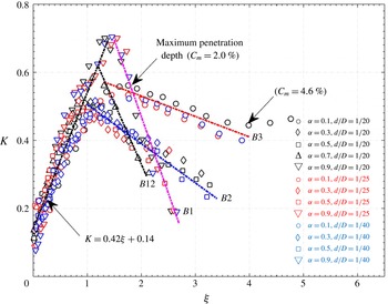
(not shown), which displays a collapse of the data and is approximately piecewise linear, albeit branched. Therefore, the data are replotted in figure 22 showing the dependence of
 $K$
on
 $(\sqrt{MR}/\unicode[STIX]{x1D6FC})(d/D)^{n}$
. All the data are from Category I or the left-hand side of the vertical broken line in figure 19, with the additional data of
 $\unicode[STIX]{x1D6FC}=0.7$
. The data of
 $K$
display a quite good collapse up to
 $\unicode[STIX]{x1D709}\equiv (\sqrt{MR}/\unicode[STIX]{x1D6FC})(d/D)^{n}\approx 1.0$
but branch into four, i.e.
 $B1$
,
 $B2$
,
 $B3$
and
 $B12$
for
 $\unicode[STIX]{x1D709}>1.0$
. The data are piecewise least-squares fitted to linear curves, viz.
 $$\begin{eqnarray}\displaystyle & \displaystyle K=0.42\unicode[STIX]{x1D709}+0.14\quad \text{for}~0\leqslant \unicode[STIX]{x1D709}\leqslant 1.0{-}1.5~(\text{depending on }\unicode[STIX]{x1D6FC}\text{ and }d/D), & \displaystyle\end{eqnarray}$$
 $$\begin{eqnarray}\displaystyle & \displaystyle B1:\quad K=-0.45\unicode[STIX]{x1D709}+1.37\quad \text{for}~\unicode[STIX]{x1D709}>1.5, & \displaystyle\end{eqnarray}$$
 $$\begin{eqnarray}\displaystyle & \displaystyle B2:\quad K=-0.12\unicode[STIX]{x1D709}+0.65\quad \text{for}~\unicode[STIX]{x1D709}>1.0, & \displaystyle\end{eqnarray}$$
 $$\begin{eqnarray}\displaystyle & \displaystyle B3:\quad K=-0.07\unicode[STIX]{x1D709}+0.62\quad \text{for}~\unicode[STIX]{x1D709}>1.0, & \displaystyle\end{eqnarray}$$
 $$\begin{eqnarray}\displaystyle & \displaystyle B12:\quad K=-0.36\unicode[STIX]{x1D709}+1.05\quad \text{for}~\unicode[STIX]{x1D709}>1.0. & \displaystyle\end{eqnarray}$$
 $K$
may deviate from the calculation from (5.2) by no more than 10 %, with a 95 % confidence; the only exception is
 $\unicode[STIX]{x1D709}<0.2$
where the deviation may go up to
 $\pm$
15 %.
Dependence of the centreline mean velocity jet decay rate
 $K$
on
 $\unicode[STIX]{x1D709}=(\sqrt{MR}/\unicode[STIX]{x1D6FC})(d/D)^{n}$
where
 $n=0.25$
–0. All the data are from the left-hand side of the local peak line in figure 19.

Before discussing the results in figure 22, we need to understand physically
 $(d/D)^{n}$
. Take the case of
 $d/D=1/20$
and
 $1/40$
for example. As
 $d/D$
is reduced from
 $1/20$
to
 $1/40$
,
 $C_{m}$
required to achieve a predefined
 $K$
, say 0.3, should be less based on figure 18. We define a percentage reduction by
 $$\begin{eqnarray}\displaystyle \unicode[STIX]{x0394}C_{m_{d/D}}=1-\frac{[C_{m}]_{1/40}}{[C_{m}]_{1/20}}, & & \displaystyle\end{eqnarray}$$
where subscripts
 $1/40$
and
 $1/20$
denote diameter ratios (
 $d/D$
). The required
 $C_{m}$
for given
 $K$
,
 $\unicode[STIX]{x1D6FC}$
and
 $d/D$
can be calculated from (5.2a
):
 $$\begin{eqnarray}\displaystyle K\approx \frac{\sqrt{MR}}{\unicode[STIX]{x1D6FC}}\left(\frac{d}{D}\right)^{n}\approx \frac{C_{m}}{\unicode[STIX]{x1D6FC}}\left(\frac{D}{d}\right)^{1-n}, & & \displaystyle\end{eqnarray}$$
or
 $$\begin{eqnarray}\displaystyle C_{m}\approx K\unicode[STIX]{x1D6FC}\left(\frac{d}{D}\right)^{1-n}. & & \displaystyle\end{eqnarray}$$
Then
 $\unicode[STIX]{x0394}C_{m_{d/D}}$
can be obtained by substituting (5.5) into (5.3) for the corresponding
 $d/D$
. The variation in
 $\unicode[STIX]{x0394}C_{m_{d/D}}$
with
 $\unicode[STIX]{x1D6FC}$
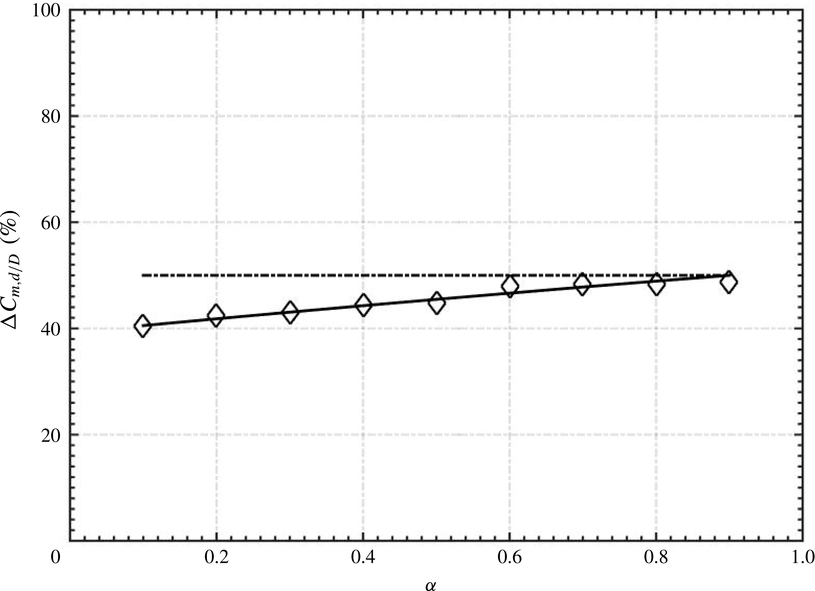
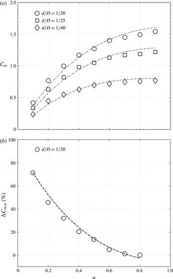
is shown in figure 23. A decrease in
 $d/D$
by half results in a drop in the required
 $C_{m}$
by approximately half (
 $\unicode[STIX]{x0394}C_{m_{d/D}}\approx 50\,\%$
) for
 $\unicode[STIX]{x1D6FC}\geqslant 0.7$
.
 $\unicode[STIX]{x0394}C_{m_{d/D}}$
contracts to 0.4 or 40 % for
 $\unicode[STIX]{x1D6FC}=0.1$
. The fact that additional
 $C_{m}$
, proportional to
 $(d/D)^{-n}$
(5.5), is required to achieve a given
 $K$
due to a reduced
 $d/D$
is physically due to the increased retardation effect of the minijet orifice. A reduction in
 $\unicode[STIX]{x1D6FC}$
further amplifies this retardation effect. That is,
 $(d/D)^{-n}$
reflects physically the retardation effect in case of small
 $d/D$
or
 $\unicode[STIX]{x1D6FC}$
.
Variation in
 $\unicode[STIX]{x0394}C_{m,d/D}$
with
 $\unicode[STIX]{x1D6FC}$
as
 $d/D$
changes from
 $1/20$
to
 $1/40$
.

The scaling factor
 $\unicode[STIX]{x1D709}=(\sqrt{MR}/\unicode[STIX]{x1D6FC})(d/D)^{n}$
is physically the effective momentum ratio per pulse of the minijet and determines the level of
 $K$
. On the other hand, the penetration depth of the control jet into the main jet also determines the level of mixing (Johari et al.
Reference Johari, Pacheco-Tougas and Hermanson1999; Johari Reference Johari2006). One question arises: are the two parameters connected? Yang (Reference Yang2017) demonstrated that the penetration depth and the distribution of
 $u_{rms}^{\ast }$
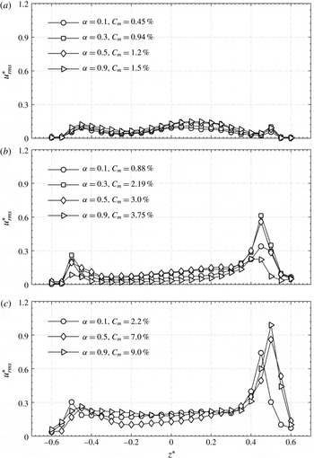
measured at the exit of the main jet are closely correlated. Figure 24 compares the
 $u_{rms}^{\ast }$
distributions across the jet, measured at
 $x^{\ast }=0.05$
, corresponding to
 $\unicode[STIX]{x1D709}\approx 0.40$
, 0.90 and 2.0. It is evident that, given the same
 $\unicode[STIX]{x1D709}$
, the
 $u_{rms}^{\ast }$
distributions are qualitatively the same despite different combinations of
 $\unicode[STIX]{x1D6FC}$
and
 $C_{m}$
. The observation suggests that the penetration depth is the same for the same
 $\unicode[STIX]{x1D709}$
, thus implying a correspondence between
 $\unicode[STIX]{x1D709}$
and the penetration depth. Furthermore, the flow structure and its downstream development are essentially the same for the same
 $\unicode[STIX]{x1D709}$
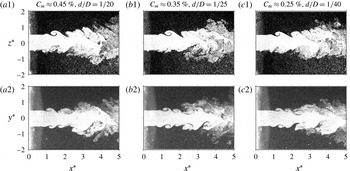
. As illustrated in figure 25, the flow structures captured at
 $\unicode[STIX]{x1D709}\approx 0.40$
in the injection and non-injection planes are qualitatively the same, including the starting roll-up position and the topological arrangement of vortices, in spite of the three different combinations of
 $C_{m}$
and
 $d/D$
. In fact, the corresponding jet mean velocity half-width
 $z_{0.5}^{\ast }$
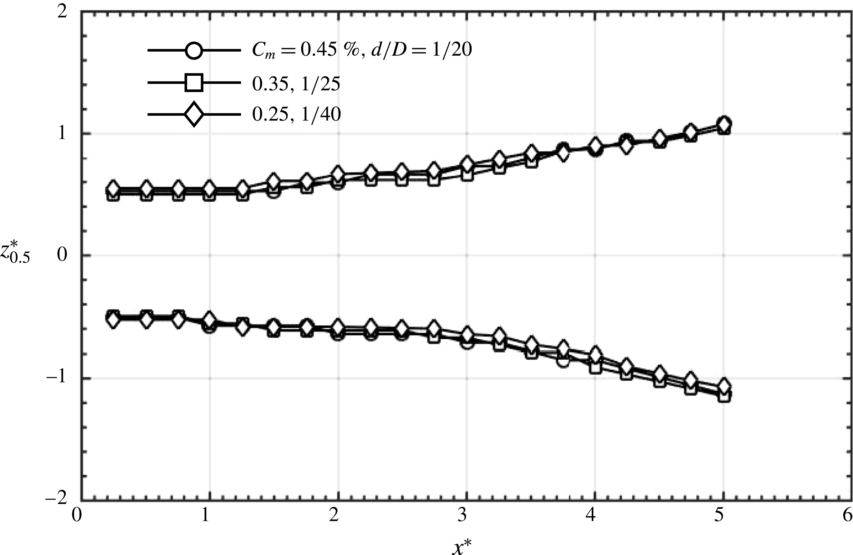
(e.g. Ball, Fellouah & Pollard Reference Ball, Fellouah and Pollard2012), measured using PIV, in the injection plane of the perturbed jet displays a good collapse over
 $x^{\ast }\approx 0$
–5 (figure 26).
Radial distributions of turbulent intensity
 $u_{rms}^{\ast }=u_{rms}/\bar{U}_{j}$
measured at
 $x^{\ast }=0.05$
(
 $f_{e}/f_{0}=0.5$
,
 $d/D=1/20$
). (a)
 $\unicode[STIX]{x1D709}\approx 0.40\pm 0.06$
; (b)
 $0.90\pm 0.06$
; (c)
 $2.0\pm 0.06$
.

Typical flow visualization photographs captured in the injection and non-injection planes of the jet (
 $\unicode[STIX]{x1D6FC}=0.1$
,
 $f_{e}/f_{0}=0.5$
) given
 $K=0.3$
and the same
 $(\sqrt{MR}/\unicode[STIX]{x1D6FC})(d/D)^{n}\approx 0.40\pm 0.06$
.

Downstream variation in the jet mean velocity half-width
 $z_{0.5}^{\ast }$
(
 $\unicode[STIX]{x1D6FC}=0.1$
,
 $f_{e}/f_{0}=0.5$
) given
 $K=0.3$
and the same
 $(\sqrt{MR}/\unicode[STIX]{x1D6FC})(d/D)^{n}\approx 0.40\pm 0.06$
:
 $d/D=1/20$
.

Typical flow structures in the injection plane of the jets from flow visualization (
 $f_{e}/f_{0}=0.5$
,
 $d/D=1/20$
) corresponding to the
 $\unicode[STIX]{x1D709}$
value in figure 20: (a)
 $\unicode[STIX]{x1D709}=(\sqrt{MR}/\unicode[STIX]{x1D6FC})(d/D)^{n}=1.8$
on curve
 $B3$
; (b) 1.0 on
 $B2$
; (c) 1.1 on
 $B12$
; (d) 1.5 on
 $B1$
.

Now let us turn to the discussion of the results presented in figure 22. For
 $\unicode[STIX]{x1D709}\leqslant 1.0$
,
 $K$
rises rapidly and almost linearly with increasing effective momentum ratio per pulse of the minijet, as expected. As an interesting comparison, Edwards, Sherman & Breidenthal (Reference Edwards, Sherman and Breidenthal1985) and Breidenthal et al. (Reference Breidenthal, Tong, Wong, Hamerquist and Landry1985) found that the decay rate of the fluctuating concentration
 $c_{rms}$
was linearly connected to the momentum ratio of the transverse jet to the rectangular duct flow. Beyond
 $\unicode[STIX]{x1D709}=1.0$
,
 $K$
may follow four distinct branches. The large deviation in
 $K$
between the branches is physically connected to the retardation experienced at large
 $\unicode[STIX]{x1D709}~({>}1.0)$
and the jet column deflection. A close look at the data in this figure unveils that the four branches are associated with distinct
 $\unicode[STIX]{x1D6FC}$
. The maximum
 $K$
of B1 exceeds considerably that of B12, B3 or B2. To understand this difference, the typical flow visualization images corresponding to the maximum
 $K$
of each branch are compared between the four cases. The maximum
 $K$
, 0.56, of B3 occurs at
 $\unicode[STIX]{x1D709}\approx 1.8$
(
 $C_{m}=2.0\,\%$
and
 $d/D=1/20$
), corresponding to the maximum penetration depth (§ 3). B3 is characterized by
 $\unicode[STIX]{x1D6FC}=0.1$
(
 $n=0.25$
), where the flow structure experiences a flapping column (figure 27
a). Physically, the minijet is encountered by a large retardation for
 $\unicode[STIX]{x1D709}>1$
. For instance, the time-averaged velocity (
 $\bar{U}_{m}$
) of minijet at
 $\unicode[STIX]{x1D709}=1.5$
and
 $\unicode[STIX]{x1D6FC}=0.1$
is
 $48~\text{m}~\text{s}^{-1}$
, but the actual velocity during the ‘on-state’ of the minijet exceeds sonic (
 $\bar{U}_{m}/\unicode[STIX]{x1D6FC}>340~\text{m}~\text{s}^{-1}$
). Evidently, branch B3 is in effect associated with partial choking given
 $\unicode[STIX]{x1D709}>1$
. Branch B2 corresponds to the
 $\unicode[STIX]{x1D6FC}$
range of 0.3–0.5 (
 $n=0.12$
–0.2). The flapping does not occur for B2 (figure 27
b), and hence its maximum
 $K$
(
 $=$
0.52 at
 $\unicode[STIX]{x1D709}=1.15$
) is smaller than that of B3. Branches B1 and B12 correspond to
 $\unicode[STIX]{x1D6FC}=0.9$
and 0.7, respectively, or the zero retardation effect (
 $n\approx 0$
). In these cases, given
 $\unicode[STIX]{x1D709}=1.0$
–2.0, the jet column appears deflected, as illustrated in figure 27(c,d). Note that branch B12 is an intermediate branch between B1 and B2 (figure 22). The deflection angle determined from the time-averaged data of 300 pairs of PIV images (not shown) is approximately
 $7^{\circ }$
(for B12, figure 27
c) and
 $10^{\circ }$
(for B1, figure 27
d) at
 $\unicode[STIX]{x1D709}\approx 1.0$
and 1.5, respectively. As
 $K$
is measured on the geometrical jet axis, the stable jet column deflection then yields an artificial increase in the maximum
 $K$
. As the vectoring angle for B12 is smaller than B1, the maximum
 $K$
for B12 is smaller than that for B1. The phenomenon of jet deflection away from the geometric axis is termed as thrust vectoring. Thrust vectoring has not been observed for jet controlled with two minijets (Davis Reference Davis1982) or symmetric injection (6 minijets, Seidel et al.
Reference Seidel, Pappart, New and Tsai2005) since asymmetric excitation is responsible for thrust vectoring (Pack & Seifert Reference Pack and Seifert2001). Beyond its maximum,
 $K$
drops almost linearly with increasing
 $\unicode[STIX]{x1D709}$
for every branch as the minijet impingement upon the opposite nozzle wall now produces turbulence (figure 5), which may affect adversely the formation and development of organized structures.
Some interesting inferences can be made from (5.2a
) to (5.2d
). Firstly, given
 $C_{m}$
,
 $f_{e}/f_{0}$
,
 $d/D$
and
 $\unicode[STIX]{x1D6FC}$
(thus
 $n$
),
 $\unicode[STIX]{x1D709}$
may be calculated and hence
 $K$
can be predicted from the equations. This may have important applications in engineering. Secondly, the required
 $C_{m}$
(figure 28
a) to achieve a pre-specified
 $K$
can be estimated from (5.2a
).
 $C_{m}$
is a practically important parameter. Following (5.3), we may define a percentage reduction as
 $\unicode[STIX]{x1D6FC}$
reduces, viz.
 $$\begin{eqnarray}\displaystyle \unicode[STIX]{x0394}C_{m_{\unicode[STIX]{x1D6FC}}}=1-\frac{[C_{m}]_{0.1{-}0.8}}{[C_{m}]_{0.9}}, & & \displaystyle\end{eqnarray}$$
where subscripts 0.1–0.8 and 0.9 denote
 $\unicode[STIX]{x1D6FC}$
. A large
 $\unicode[STIX]{x0394}C_{m_{\unicode[STIX]{x1D6FC}}}$
means a higher control efficiency (figure 28
b). For example, to achieve a pre-determined
 $K=0.3$
for
 $d/D=1/40$
,
 $C_{m}$
required may be calculated from (5.2a
), which is 0.25 % at
 $\unicode[STIX]{x1D6FC}=0.1$
, 68 % lower than that (
 $C_{m}=0.80\,\%$
) at
 $\unicode[STIX]{x1D6FC}=0.9$
calculated from (5.6). The result highlights the highly effective entrainment under the unsteady minijet excitation of small
 $\unicode[STIX]{x1D6FC}$
. Lastly, as noted earlier, the required
 $C_{m}$
drops as
 $d/D$
is reduced (figure 28
a), also implying an improved control efficiency.
Variation of (a)
 $C_{m}$
and (b)
 $\unicode[STIX]{x0394}C_{m,\unicode[STIX]{x1D6FC}}$
, with
 $\unicode[STIX]{x1D6FC}$
given
 $\unicode[STIX]{x1D709}=0.40$
or
 $K=0.3$
(
 $f_{e}/f_{0}=0.5$
).

6 Conclusions
Experimental study has been carried out to study the manipulation of a turbulent round jet with a single unsteady minijet. Four control parameters, i.e.
 $C_{m}$
,
 $f_{e}/f_{0}$
,
 $\unicode[STIX]{x1D6FC}$
and
 $d/D$
, are examined to understand their influence on the main jet. Extensive measurements are performed in three orthogonal planes of the main jet. The scaling analysis of the jet control is also performed empirically. Following conclusions are drawn from the investigation:
(i) The control performance, as indicated by
 $K$
, of the manipulated jet strongly depends on
$C_{m}$
,
$f_{e}/f_{0}$
,
$\unicode[STIX]{x1D6FC}$
and
$d/D$
, i.e.
$K=g_{1}$
(
$C_{m}$
,
$f_{e}/f_{0}$
,
$\unicode[STIX]{x1D6FC}$
,
$d/D$
). The maximum
$K$
occurs in general at
$f_{e}/f_{0}=0.5$
(figure 7), not at 1.0, regardless of
$d/D$
, primarily due to jet flapping generated at
$f_{e}/f_{0}=0.5$
but not at
$f_{e}/f_{0}=1.0$
. Given
$f_{e}/f_{0}=0.5$
and
$\unicode[STIX]{x1D6FC}=0.1$
–0.9, the variation in
$K$
with increasing
$C_{m}$
is characterized by two distinct categories: (i) a rapid rise to a local maximum at
$C_{m}=2.0\,\%{-}5.0\,\%$
followed by a drop, and (ii) a monotonic growth. The greatly increased
$K$
in the first category is largely due to the generation of the flapping motion, while the monotonic rise in
$K$
in the second category is caused by the intensified turbulence at higher
$C_{m}$
(Yang & Zhou Reference Yang and Zhou2016). The
$K$
decreases from
$\unicode[STIX]{x1D6FC}=0.1$
to 0.9, irrespective of
$C_{m}$
, although the variation is negligibly small beyond
$\unicode[STIX]{x1D6FC}>0.7$
. It has been found from the flow visualization and spectral phase data that the flapping jet column occurs for
$\unicode[STIX]{x1D6FC}=0.1$
and disappears for
$\unicode[STIX]{x1D6FC}>0.3$
. The smaller
$d/D$
is more efficient in enhancing mixing than the larger. Given
$C_{m}$
, the smaller
$d/D$
is associated with a larger penetration depth due to the increased injection velocity.
(ii) Empirical scaling analysis has demonstrated that, given a large
$\unicode[STIX]{x1D6FC}$
say 0.9, the main jet behaves as quasi-steady blowing and the dependence of the measured
$K$
on the momentum ratio
$\sqrt{MR}=C_{m}(D/d)$
of the minijet to main jet collapses for various
$d/D$
, that is,
$\sqrt{MR}$
is the controlling scaling factor. Once
$\unicode[STIX]{x1D6FC}$
is reduced to below 0.9,
$K$
varies with
$d/D$
, but the dependence on
$\sqrt{MR}$
of the rescaled
$K$
, i.e.
$K(D/d)^{n}$
, again collapses for various
$d/D$
; so does the dependence on
$f_{e}/f_{0}$
of
$K(D/d)^{n}$
. The power index
$n$
is dependent only on
$\unicode[STIX]{x1D6FC}$
and may be given by
$n=-0.31\unicode[STIX]{x1D6FC}+0.28$
for the present flow and control conditions. Thus,
$K=g_{1}$
(
$C_{m}$
,
$f_{e}/f_{0}$
,
$\unicode[STIX]{x1D6FC}$
,
$d/D$
) is reduced to one similarity parameter,
$\unicode[STIX]{x1D709}=(\sqrt{MR}/\unicode[STIX]{x1D6FC})(d/D)^{n}$
, where dimensionless parameters
$\sqrt{MR}/\unicode[STIX]{x1D6FC}$
and
$(D/d)^{n}$
are physically the momentum per pulse of the minijet and the resistance/retardation to fluid flowing through the minijet orifice, respectively. For
$\unicode[STIX]{x1D6FC}\geqslant 0.7$
,
$n\approx 0$
, that is, the retardation effect is negligibly small. For unsteady injection, this retardation increases with a decrease in
$d/D$
as the
$C_{m}$
required to achieve a pre-determined
$K$
is simply governed by
$\sqrt{MR}$
or
$(D/d)$
for
$\unicode[STIX]{x1D6FC}\geqslant 0.7$
but
$\sqrt{MR}(d/D)^{n}$
for
$\unicode[STIX]{x1D6FC}<0.7$
. For example, a decrease in
$d/D$
by half results in a decrease in the required
$C_{m}$
by 50 % for
$\unicode[STIX]{x1D6FC}\geqslant 0.7$
but a decrease in
$C_{m}$
by 40 %, rather than 50 % (figure 23), for
$\unicode[STIX]{x1D6FC}=0.1$
. The fact that some additional
$C_{m}$
, proportional to
$(d/D)^{-n}$
, is required to achieve a pre-defined
$\unicode[STIX]{x1D709}$
is physically due to the retardation effect.(iii) The scaling relation branches into four,
$B1$
,
$B2$
,
$B12$
and
$B3$
, beyond
$\unicode[STIX]{x1D709}>1.0$
.
$B1$
corresponds to
$\unicode[STIX]{x1D6FC}=0.9$
or above, i.e. the quasi-steady blowing or zero retardation effect (
$n=0$
).
$B2$
corresponds to
$\unicode[STIX]{x1D6FC}=0.3$
–0.5 or a moderate retardation (
$n=0.06$
–0.20).
$B12$
is an intermediate branch between
$B1$
and
$B2$
, corresponding to
$\unicode[STIX]{x1D6FC}=0.7$
.
$B3$
is associated with
$\unicode[STIX]{x1D6FC}=0.1$
or a high retardation (
$n=0.25$
), under which the minijet is partially choked at
$\unicode[STIX]{x1D709}>1.0$
where
$C_{m}$
is large. There is a considerable difference in the maximum
$K$
between the four branches. Branches B3 and B2 are characterized by flapping and non-flapping jet columns, respectively. It is the flapping motion that is responsible for the larger maximum
$K$
of B3 than that of B2. On the other hand, the jet columns of B1 and B12 deflect away from the geometric axis, experiencing the thrust vectoring phenomenon. This deflection produces an artificial increase for
$K$
and hence their maximum
$K$
values exceed those of B3 and B2.(iv) The similarity parameter
$\unicode[STIX]{x1D709}$
or the effective momentum per pulse of injection may be further interpreted as the effective penetration depth. Given the same
$\unicode[STIX]{x1D743}$
, the flow structure and its downstream development are essentially the same; for instance, the streamwise variation in the jet mean velocity half-width
$z_{0.5}^{\ast }$
collapses well over
$x^{\ast }\approx 0$
–5, irrespective of different combinations of
$C_{m}$
and
$d/D$
.(v) Given
$\unicode[STIX]{x1D709}$
or
$K$
, the required
$C_{m}$
drops as the duty cycle or the minijet injection diameter is reduced, that is, the control efficiency is improved. For example, a 68 % reduction in required
$C_{m}$
is achieved at
$\unicode[STIX]{x1D6FC}=0.1$
compared to that at
$\unicode[STIX]{x1D6FC}=0.9$
, which highlights the highly effective entrainment under the unsteady minijet excitation of small
$\unicode[STIX]{x1D6FC}$
; a decrease in
$d/D$
by half results in a decrease in the required
$C_{m}$
by 40 % (
$\unicode[STIX]{x1D6FC}=0.1$
), that is, the choice of
$d/D$
may have an important impact on jet mixing. The penetration depth, flow structure and its downstream development are found to be the same, irrespective of different
$C_{m}$
and
$d/D$
, as long as
$\unicode[STIX]{x1D709}$
is unchanged. The required momentum ratio or
$C_{m}$
at given
$d/D$
and
$\unicode[STIX]{x1D6FC}$
to achieve a pre-determined
$\unicode[STIX]{x1D709}$
or
$K$
can be calculated from the scaling relation (figure 22).











Acknowledgements
Y.Z. wishes to acknowledge support given to him from NSFC through grants 11632006 and U1613226 and A.K.P. acknowledges the support from Research Grants Council of Shenzhen Government through grant JCYJ20160531193220561.
Appendix A. Incompressible assumption
To check the validity of incompressible assumption, we compare the
 $\bar{U}_{m}$
values estimated using incompressible and compressible equations.
 $\bar{U}_{m}$
can be calculated from the equation
 ${\dot{m}}_{m}=\unicode[STIX]{x1D70C}_{m}A_{m}\bar{U}_{m}$
given
 ${\dot{m}}_{m}$
and
 $\unicode[STIX]{x1D70C}_{m}$
, where
 $\unicode[STIX]{x1D70C}$
and
 $A$
denote the density of the fluid medium (air) and exit area of the minijet, respectively. If the minijet flow is compressible,
 $\unicode[STIX]{x1D70C}_{m}$
is unknown and hence
 ${\dot{m}}_{m}$
can be rewritten, with
 $\unicode[STIX]{x1D70C}_{m}$
eliminated, as following (see equation (4.16) in Shapiro Reference Shapiro1953),
 $$\begin{eqnarray}\displaystyle {\dot{m}}_{m}=\frac{A_{m}P_{0}}{\sqrt{T}_{0}}\sqrt{\frac{\unicode[STIX]{x1D6FE}}{R}}M_{m}\left(1+\frac{\unicode[STIX]{x1D6FE}-1}{2}M_{m}^{2}\right)^{-((\unicode[STIX]{x1D6FE}+1)/(2(\unicode[STIX]{x1D6FE}-1)))}, & & \displaystyle\end{eqnarray}$$
where,
 $P_{0}$
,
 $T_{0}$
,
 $\unicode[STIX]{x1D6FE}$
,
 $R$
and
 $M_{m}$
represent the stagnation pressure, stagnation temperature for the minijet, specific heat ratio, gas constant and Mach number at the minijet exit, respectively.
 $P_{0}$
is unknown in (A 1), which can be replaced from the following isentropic equation, viz.
 $$\begin{eqnarray}\displaystyle \frac{P_{0}}{P}=\left(1+\frac{\unicode[STIX]{x1D6FE}-1}{2}M_{m}^{2}\right)^{\unicode[STIX]{x1D6FE}/(\unicode[STIX]{x1D6FE}-1)}, & & \displaystyle\end{eqnarray}$$
where
 $P$
is the atmospheric pressure. On rearranging,
 $$\begin{eqnarray}\displaystyle {\dot{m}}_{m}=\frac{A_{m}P}{\sqrt{T}_{0}}\sqrt{\frac{\unicode[STIX]{x1D6FE}}{R}}M_{m}\left(1+\frac{\unicode[STIX]{x1D6FE}-1}{2}M_{m}^{2}\right)^{1/2}. & & \displaystyle\end{eqnarray}$$
For a given
 ${\dot{m}}_{m}$
,
 $M_{m}$
can be calculated from (A 3), noting the predefined ‘
 $d=1$
mm’,
 $p=1$
atm,
 $\unicode[STIX]{x1D6FE}=1.4$
and
 $R=287~\text{J}~\text{kg}^{-1}~\text{K}^{-1}$
. Then, from isentropic equation,
 $$\begin{eqnarray}\displaystyle \frac{T_{0}}{T}=1+\frac{\unicode[STIX]{x1D6FE}-1}{2}M_{m}^{2}. & & \displaystyle\end{eqnarray}$$
From Mach number relation,
 $$\begin{eqnarray}\displaystyle \bar{U}_{m}=M_{m}\sqrt{\unicode[STIX]{x1D6FE}RT}. & & \displaystyle\end{eqnarray}$$
Finally,
 $\bar{U}_{m}$
can be determined from (A 5) from the known
 $M_{m}$
(A 3) and
 $T$
(A 4). Note that
 $T_{0}=298$
K in the settling chamber.
Variation in
 $\bar{U}_{m}$
with
 $C_{m}$
for
 $d/D=1/20$
.

To determine the error involved in assuming the minijet flow to be incompressible, we calculate
 $\bar{U}_{m}$
for incompressible flow and compare it with
 $\bar{U}_{m}$
calculated from (A 5).
 $$\begin{eqnarray}\displaystyle C_{m}=\frac{{\dot{m}}_{m}}{{\dot{m}}_{j}}=\frac{\unicode[STIX]{x1D70C}_{m}}{\unicode[STIX]{x1D70C}_{j}}\frac{A_{m}}{A_{j}}\frac{\bar{U}_{m}}{\bar{U}_{j}}. & & \displaystyle\end{eqnarray}$$
Assuming incompressible flow and rearranging (A 6) yield
 $$\begin{eqnarray}\displaystyle \bar{U}_{m}=C_{m}\left(\frac{D}{d}\right)^{2}\bar{U}_{j}. & & \displaystyle\end{eqnarray}$$
Figure 29 compares
 $\bar{U}_{m}$
obtained from the incompressible assumption (A 7) with that from (A 5), where subscripts IC and
 $C$
denote incompressible and compressible assumptions, respectively. It is evident that for
 $C_{m}<4.2\,\%$
the deviation in
 $\bar{U}_{m}$
between the two assumptions is approximately zero. For
 $4.2\,\%<C_{m}<8.2\,\%$
, this deviation is no more than 3 %. The present scaling analysis considered for Category I falls within
 $0<C_{m}<8.2\,\%$
. As such, the error associated with the use of equation
 $MR={\dot{m}}_{m}\bar{U}_{m}/{\dot{m}}_{j}\bar{U}_{j}=({\dot{m}}_{m}/{\dot{m}}_{j})^{2}(\unicode[STIX]{x1D70C}_{m}/\unicode[STIX]{x1D70C}_{j})(A_{j}/A_{m})=C_{m}^{2}(D/d)^{2}$
does not exceed 3 %.