


The Great Depression featured a severe, nationwide housing crisis. Housing construction contracted far more than economic activity in general, recovered more slowly, and accounted for nearly 30 percent of the fall in investment between 1929 and 1933.Footnote 1 Housing prices and employment both collapsed, leading to a nationwide foreclosure crisis and a decline in home ownership on a scale not approached again until the 2007–2009 financial crisis. At the same time, mortgage credit dried up in spectacular fashion. A key source of the Depression mortgage credit crunch was the accumulation of crushingly large amounts of foreclosed real estate on lenders’ balance sheets, reducing their capacity to engage in new lending given the illiquidity and low returns from that real estate.
Bernanke (Reference Bernanke1983) argued that frictions in the commercial banking sector during the Great Depression operated through a financial mechanism that accelerated the forces of economic contraction. A number of scholars have continued to flesh out the frictions in commercial banking during the Great Depression, but none has had the data to measure the impact of foreclosures on new lending.Footnote 2 Further, that important body of work tells us very little about the frictions in Depression housing markets because commercial banks accounted for only a small share of home lending.Footnote 3 The leading mortgage lenders in the 1920s and early 1930s were building and loans (B&Ls), which were organized as mutual associations in which home borrowers held significant ownership stakes. In fact, Bernanke (Reference Bernanke1983) noted substantial problems in the B&L sector but focused his attention on commercial banks instead. This paper represents the first attempt to address his hypothesis that distressed mortgage lenders were constrained in their ability to engage in new lending during the Depression’s severe and prolonged housing crisis.
We have collected firm-level data on the annual balance sheets of hundreds of individual B&Ls, covering every B&L operating between 1928 and 1940 in four states: Iowa, New York, North Carolina, and Wisconsin. One major advantage of the data from these states is the availability of information on the volume of new mortgage lending each year. Most studies of financial institutions do not have this direct measure and instead rely on changes in the value of outstanding loans as a proxy for new lending. Such a proxy is subject to substantial measurement error because repayment of loans and foreclosures also lead to changes in outstanding loan values. We show that using the more accurate measure of new lending flows leads to materially different and more precise estimates than using changes in loan stocks.
We examine the relationship between new lending and foreclosures using this panel, controlling for a broad range of factors. B&L fixed effects control for time-invariant B&L characteristics, and county-by-year fixed effects control for changes in local economic conditions that influenced incomes, demand for housing, costs of building housing, and refinancing activity by the Home Owners’ Loan Corporation (HOLC). Therefore, the results are driven by changes within B&Ls over time that are uncorrelated with annual fluctuations in county-level demand and supply factors. Information on lagged assets and the liability structure of B&Ls controls for firm-specific restrictions on lending that might arise from the nature of its holdings, obligations, or business models. These factors also control, to some extent, for housing market changes at the neighborhood level for small B&Ls that are not captured by the county-by-year fixed effects. We also control for a variety of government interventions and transitions from state-level B&L charters to the new federal savings and loan (S&L) charters. Altogether, the relationship between new loans and real estate owned (REO) can be considered causal if there are no uncontrolled firm-specific subcounty time-varying shocks that influence both loans and foreclosures. Following the approach of Altonji, Elder, and Taber (Reference Altonji, Elder and Taber2015) and Oster (Reference Oster2019), we show that the influence of such unmeasured factors would have to be stronger, by a factor of three, than the influence of observable factors to be able to explain the estimated relationship.
The results show that an increase in foreclosed real estate on a B&L’s balance sheet, known as REO, strongly reduced new mortgage lending during the 1930s. A one-standard-deviation rise in REO as a share of assets was associated with a 5-percentage-point drop in new loans as a percentage of assets. Such a drop was nearly one-third of the mean value of the ratio of new loans to assets among B&Ls. The impact of REO was felt throughout the crisis but changed in character during the decade. Between 1929 and 1935, the increase in the mean REO share accounted for 30 percent of the drop in the mean new loan share in the sample. In contrast, the REO mean share of B&L assets remained elevated throughout the last half of the decade, with only a small reduction that accounted for 5 percent of the total increase in new loans. The results are the first empirical examination of the mechanism behind the credit crunch that occurred in 1930s mortgage markets. They are also the first measurement of impact of loan foreclosures on new lending for any type of financial institution during the Great Depression.Footnote 4 This credit crunch mechanism was substantial despite the multifaceted and aggressive intervention in the mortgage market by the federal government in the 1930s.
This historical setting is emblematic of a credit market dominated by portfolio lenders who held on to the loans they made. This contrasts sharply with the modern U.S. mortgage market in which most loans are sold and incorporated into securities (Snowden Reference Snowden, Mitchell and Wilmarth2010). The 2007–2009 financial crisis demonstrated the potential fragility underlying securitization structures. That crisis raised the question of whether the problems of the 2000s might not have occurred if lenders had held on to their loans rather than selling them into the securitization market. This paper underscores that portfolio lenders who hold on to their loans also can face fragile conditions that can lead to credit crunches that deepen downturns.Footnote 5
WHAT WE KNOW ABOUT THE DEPRESSION HOUSING CRISIS
Aggregate data show enormous setbacks in housing and housing finance during the Depression. Housing starts dropped 85 percent between 1929 and 1933, compared to a 30 percent drop in real gross domestic product (GDP). Starts also failed to recover to their 1929 level until 1940, while real GDP had recovered to its 1929 level by 1936. Median nominal home values fell roughly 18–32 percent between 1930 and 1940 for the nation, and by at least 25 percent in 80 percent of the nation’s counties. More to the point of this paper, 10–20 percent of mortgaged homeowners experienced a foreclosure between 1926 and 1936, while new lending volumes by all classes of lenders throughout the 1930s remained, at most, half of the level of the late 1920s. Finally, residential mortgage debt as a share of total mortgage debt fell from 34 to 24 percent between 1934 and 1940, while the nonfarm homeownership rate fell from 45 to 40 percent between 1930 and 1940.Footnote 6
The Depression residential mortgage crisis was well known to contemporaries and was met by a massive policy response. These efforts included the establishment of the Federal Home Loan Bank (FHLB) System, state-level mortgage moratoria laws, the HOLC, the Federal Housing Administration, insurance for S&L investments, new federal charters for S&L associations, and the creation of Fannie Mae. Altogether, while the federal government entered the Depression with essentially no role in the nation’s housing market, by the mid-1930s, it had fundamentally reshaped the institutional structure of that market. Below, we examine how participation of B&Ls in these programs affected the impact of foreclosures on new lending.
From the late 1930s to the 1950s, economists published many studies on the Depression housing finance crisis (Snowden Reference Snowden, White, Snowden and Fishback2014). Interest in the Depression-era developments in housing finance began to wane in the 1960s, while the banking sector received renewed attention, particularly because of the work of Friedman and Schwartz (1963). Bernanke (Reference Bernanke1983) turned the voluminous literature on banking toward financial frictions, and since then, a large number of papers have yielded many insights into sources and consequences of commercial bank fragility during the Depression.Footnote 7
Economists in the early postwar period also focused on the concept of a more general “building cycle” across American economic history (Abramovitz Reference Abramovitz1964; Hansen Reference Hansen1964) and the integral nature of construction and building for the macroeconomy (Hickman Reference Hickman, David and Reder1973). Since then, economic historians have also examined apparent “overbuilding” and “unplanned development” (Bolch, Fels, and McMahon Reference Bolch, Fels and McMahon1971; Field Reference Field1992).
Since the 2007–2009 financial crisis, researchers have shown more interest in subjects related to the Depression-era credit crunch in mortgage markets. One topic of inquiry is the extent to which the refinancing available through the HOLC was able to partially ameliorate the mortgage credit crunch of the 1930s and improve outcomes for home mortgage borrowers. In addition, researchers have described the factors that led to a protracted resolution for troubled lenders, especially relative to the disruptions in the commercial banking sector.Footnote 8
The mortgage credit crunch itself has been described in aggregate terms by Field (Reference Field, White, Snowden and Fishback2014), White (Reference White, White, Snowden and Fishback2014), and Gjerstad and Smith (Reference Gjerstad, Smith, White, Snowden and Fishback2014a). More recently, Cortes and Weidenmier (Reference Cortes and Weidenmier2019) have found that building permits can predict stock market volatility during the Great Depression. However, with aggregate data, it is difficult to assess the mechanisms at work behind the credit crunch. The impressions of industry insiders during the 1930s were that foreclosures and the resulting REO represented a direct and immediate barrier to the supply of new loans quite apart from any feedback effect they may have had on local loan demand.Footnote 9 The disaggregated B&L-level data available in this paper allow for a direct investigation of those underlying causes. Indeed, we are the first to gather data on individual B&Ls in the 1930s.
Finally, the literature on the recovery from the Great Depression (not specific to the mortgage market) has also grown in recent years. Fishback (Reference Fishback2017) provides a survey of the growing literature on the impact of the New Deal. Several papers have focused narrowly on the sharp turnaround during the spring of 1933, including Hausman, Rhode, and Wieland (Reference Hausman, Rhode and Wieland2019), Taylor and Neumann (Reference Taylor and Neumann2016), Jalil and Rua (Reference Jalil and Rua2016), and Eggertsson (Reference Eggertsson2008). Other papers examine the longer period of recovery that lasted up to WWII, including Fishback, Horrace, and Kantor (Reference Fishback, Horrace and Kantor2005) and Fishback and Kachanovskaya (Reference Fishback and Kachanovskaya2015). For the most part, these papers focus on inflationary expectations and nonfinancial microeconomic variables. In contrast, this paper looks at the role of continued financing frictions within the residential mortgage sector, which has not been studied.
B&L ASSOCIATIONS AND THE MORTGAGE CREDIT CRUNCH
In analyzing new residential mortgage lending in the 1930s, we stress the importance of three facts about B&Ls and the residential finance sector.
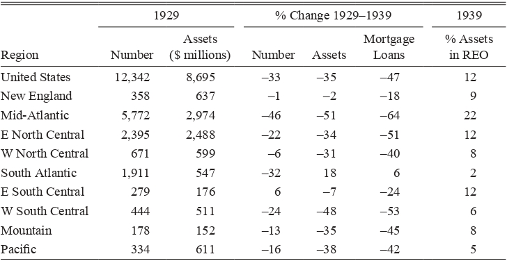
First, B&Ls were the key actors. In the 1920s, B&Ls were the primary institutional source of mortgage funds in the interwar United States. By 1929, more than 12,000 B&Ls were operating in every state and region and in cities of all sizes (Bodfish Reference Bodfish1931; Snowden Reference Snowden, Engerman, Hoffman, Rosenthal and Sokoloff2003). At that point, B&Ls accounted for 48 percent of the mortgage debt held by institutional lenders on the nation’s 1–4 family homes. From 1929 and 1934, the amount of new loans made by B&Ls fell by two-thirds (adjusted for rent consumer price index (CPI) inflation) and other lenders generally did not pick up the slack.Footnote 10
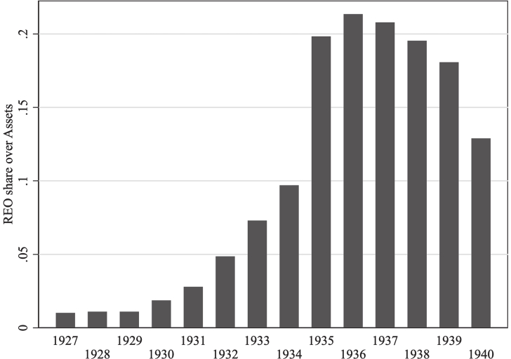
Second, the B&Ls’ institutional structure did little to insulate their new lending from an overhang of foreclosed real estate. B&L assets consisted more or less exclusively of housing loans; as a result, they had little diversity in assets to help buffer the shocks from real estate lending. Figure 1 shows that B&L REO, largely due to foreclosures, peaked at an astonishing 20 percent of assets in the four states we observe. In addition, illiquidity and even insolvency did not necessarily trigger their forced closure because borrowers accounted for a significant share of B&L ownership. Fleitas, Fishback, and Snowden (Reference Fleitas, Fishback and Snowden2018) show that B&Ls were slow to liquidate and reorganize because their bylaws and case law required the support of two-thirds of the members in a vote before the institution could be liquidated. Borrower members and nonborrowing members had equal voting rights, and they had strong incentives to delay liquidation because they could avoid significant losses by repaying their loans before their B&Ls liquidated. Consequently, many B&Ls staggered into the late 1930s with enormous amounts of real estate on their books, still operating and attempting to make new loans.
REO AS A PERCENT OF ASSETS AT B&L ASSOCIATIONS IN IOWA, NEW YORK, NORTH CAROLINA, AND WISCONSIN, 1927–1940
Third, the federal government intervened aggressively in the 1930s in residential mortgage markets, but nevertheless, the burden of REO on lenders remained very large. The FHLB system and the Reconstruction Finance Corporation (RFC) had potential to reduce the liquidity constraints on lenders, but the FHLB made real estate ineligible as collateral; not much is known about the RFC lending program among real estate lenders. The HOLC refinanced nearly one-fifth of all residential mortgages in the country, but also rejected a roughly equal number of applications, leaving substantial amounts of foreclosed real estate on the balance sheets of B&Ls and other intermediaries. The consensus of recent evidence suggests that the HOLC partially ameliorated but did not reverse the negative impact of the crisis on home values, ownership, and construction (Fishback et al. Reference Fishback, Kantor, Flores-Lagunes, Horrace and Treber2011; Courtemanche and Snowden Reference Courtemanche and Snowden2011; see also Harriss Reference Harriss1951; Fishback, Rose, and Snowden Reference Fishback, Rose and Snowden2013). Finally, B&Ls used the Federal Housing Administration program less than any other major lending group during the 1930s and the decades that followed (Ewalt Reference Ewalt1962, pp. 134–45).
DATA AND DESCRIPTIVE STATISTICS
The data analyzed here include annual balance sheet data and new real estate loan volume for every state-chartered B&L association that operated in Iowa, New York, and North Carolina between 1928 and 1940 and in Wisconsin between 1935 and 1940. In a robustness check, we also use data from newly chartered federal associations in the latter half of the 1930s. The appendix provides a full description of our data sources, which are annual reports by state and federal regulators. The data and replication files can be found in Fishback et al. (Reference Fishback, Fleitas, Rose and Snowden2020).
We use data from these four states because they are the only ones that reported both the volume of new loans and balance sheet data in these years. The availability of data on new loans is unusual and quite valuable for our analysis. It is common in the banking literature to use annual changes in the stock of loans as a measure of new lending, but this approach is inappropriate for mortgage specialists such as B&Ls. New mortgage lending would be understated, for example, when early repayments or defaults and foreclosures reduced the stock of mortgage loans. Both possibilities were likely to have been at work for B&Ls during the 1930s. The sinking fund mortgage loan contract used by these intermediaries provided strong incentives for borrowers with sufficient resources to repay early. By doing so, they avoided sharing in the losses earned by their associations (Fleitas, Fishback, and Snowden Reference Fleitas, Fishback and Snowden2018). The increase in foreclosures of interest here, moreover, depressed the stock of loans held by B&Ls throughout the 1930s. So too did purchases of distressed loans by the HOLC. For all of these reasons, changes in the stock of loans would be a poor and noisy proxy for new lending by B&Ls in the 1930s. We focus only on institutions in states for which new lending each year was reported in regulatory reports. We show below, in fact, that our central empirical results cannot be precisely or consistently estimated using annual changes in the stock of loans as a proxy for new loans.
Although Wisconsin did not start to report annual lending until 1935, we included it in the sample to incorporate information from a state in the East North Central region along with information from the Mid-Atlantic (New York), the West North Central (Iowa), and the south Atlantic (North Carolina). As shown in Table 1, these four regions (out of nine) claimed 87 percent of the nation’s B&Ls in 1930 and 76 percent of the industry’s assets. These four areas also capture the marked regional variation in disruption experienced within the B&L industry during the 1930s. Finally, all four states in our sample claimed substantial B&L sectors and large and diverse economies. According to the 1930 census, these states all had significant numbers of manufacturing, construction, and agricultural workers.
THE B&L INDUSTRY IN 1929–1939
Note: The dollar figures are not adjusted for inflation.
Sources: The data come from three editions of the Monthly Labor Review: November (1930, pp. 114–15), January (1941, pp. 126–27), and May (1943, p. 937); the Federal Home Loan Bank Board, Eighth Annual Report (1940, pp. 175–76); and the Federal Home Loan Bank Board, Ninth Annual Report (1941, pp. 242–45).
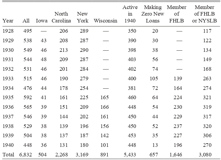
Table 2 provides an overview of the composition of the B&L panel across states and over time. All four states saw the number of state-chartered B&Ls decrease during the 1930s. Most of these exits resulted from voluntary liquidations, but one-sixth occurred when operating B&Ls were granted federal S&L charters. Most of these charter conversions were in New York. Altogether, 262 of 859 B&Ls in the sample exited at some point, while 597 remained in operation in 1940, including the 53 that had converted to federal S&L charters.
B&Ls IN SAMPLE REPORTING NEW LOANS
Source: The data come from reports of state B&L regulators (see the Appendix).
The number of active B&Ls each year that made no new mortgage loans rose to 118 by 1933 before slowly declining over the rest of the decade. Descriptive histories of B&Ls during the crisis emphasized the existence of “frozen” associations that were so severely distressed that they ceased making loans and operated for years only to manage foreclosures, to service existing loans, and to pay off withdrawing nonborrowers (Ewalt Reference Ewalt1962, pp. 16–18). The last two columns of Table 2 report the number of B&Ls that were members of the new FHLB system after 1932 or either the FHLB or the similar New York state system that was established in the mid-1920s.
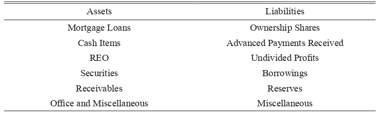
To provide comparability across states and times in the empirical work presented here, we organized all reported balance sheet variables into six categories each of assets and liabilities, as shown in Table 3. Each of these is a heterogeneous aggregate. Mortgage loans, for example, include the traditional sinking fund B&L loans and the direct reduction loan that became popular late in the decade. Ownership shares, on the other hand, include traditional B&L installment shares as well as varieties of prepaid shares that gained popularity in the 1920s. The REO aggregate includes not only foreclosed real estate, but also real estate deeded to a B&L in lieu of foreclosure, judgments for real estate not yet foreclosed upon, and real estate contracts for foreclosed properties sold on credit. The B&Ls in our sample, as was generally the case in the industry, entered the 1930s with mortgage loans representing 90 percent of assets and member shares representing a similar share of liabilities.
ASSETS AND LIABILITIES CATEGORIES
Source: Stylized balance sheet as summarized by the authors.
In bad times, such as the 1930s, loans were foreclosed upon and replaced on the balance sheet with REO. Figure 1 shows that REO accounted for only one percent of B&Ls’ assets in the 1920s but reached roughly 20 percent of assets by the mid-1930s. Figure 2 shows that new lending fell during the early 1930s and then slowly climbed back up. High-REO B&Ls (those for which REO accounts for more than 10 percent of assets in the previous year) exhibit a more rapid decline in lending and a slower recovery in each year compared to low-REO B&Ls. Our empirical estimation explores this variation further.
NEW MORTGAGE LENDING AT B&LS, BY LEVEL OF REO

EMPIRICAL APPROACH
Our empirical approach estimates how the annual flow of new loans from B&Ls was influenced by the holding of foreclosed real estate between 1928 and 1940. The mechanism was relatively simple. Relative to the mortgage loans that generally dominated the assets of a healthy B&L, foreclosed real estate earned lower average returns, often represented unrealized losses, and was generally illiquid even when a B&L was willing to recognize the loss. As a result, foreclosed real estate directly decreased the pool of loanable funds generated by a B&L’s existing mortgage portfolio and made new and additional investments in the association less attractive to nonborrowing savers. Our focus is on estimating the relationship between the B&L’s new lending and the share of assets soaked up by foreclosed real estate.
To assess the magnitude of this disruption to B&L mortgage lending, we estimate the following regression equation:
 $$NewLoan{s_{ijt}} = {\delta _i} + {\alpha _1}RE{O_{ijt - 1}} + \ln {S_{ijt - 1}}{\beta _1} + {L_{ijt - 1}}{\beta _2} + {\mu _{jt}} + {\varepsilon _{ijt}}$$
In this equation, NewLoans ijt is the value of new loans as a percentage of the value of assets in firm i in county j in year t. REO ijt–1 is REO as a share of assets in the prior year. Therefore, α 1 is the coefficient of interest; it shows the correlation between the new loan share and the shift toward real estate holdings in the assets after controlling for the other correlates.
The coefficient α 1 can be given a causal interpretation if there are no unmeasured factors in the error term that are correlated with both the lagged REO share and new loans share. Therefore, our empirical strategy is to include in the specification multiple controls that are designed to soak up any factors that would otherwise be in the error term and that may be correlated with new lending. Overall, our identification assumption is that the changes in lagged REO within the same B&L over time are uncorrelated with unobserved shocks to new lending, after accounting for an exhaustive set of controls.
First among our controls are two sets of fixed effects. A firm fixed effect (δ i) controls for unchanging features of the B&L, including their locations, by-laws, and other structural features. These might include locations near prime neighborhoods or the quality of long-term managers who could influence the cost of foreclosing loans, selling property, making new loans, or attracting investors and borrowers. Second, a full set of county-by-year fixed effects (μ jt) controls for factors, such as economic activity, housing market status, and government policies, at the county level over time (Fishback and Kachanovskaya Reference Fishback and Kachanovskaya2015; Fishback, Horrace, and Kantor Reference Fishback, Horrace and Kantor2005). Therefore, the remaining variation comes from changes within B&Ls over time distinct from trends across all B&Ls in a county.
Third, we control for each B&L’s balance sheet characteristics, including size (lnS ijt–1, the log of total assets) and a set of variables measuring the composition of each B&L’s assets and liabilities (A ijt–1 and L ijt–1, the share of assets and liabilities in each of our six asset categories and six liability categories listed in Table 3, with miscellaneous assets and miscellaneous liabilities omitted to avoid perfect multicollinearity). We lag balance sheet information one year to avoid the simultaneity created by mechanical links in balance sheet composition. We control for the size of an association as it may be correlated with features of its business model, such as the sophistication of its management or the diversification of its lending, and therefore changes in size over time may affect new lending and could be correlated with REO holdings. We control for the composition of each association’s balance sheet because changes in these factors, and the underlying solvency, liquidity, and risk exposure that they measure, may affect new lending and could be correlated with changes in REO. In addition, these are also factors that are likely to capture changes in the subcounty local housing and mortgage markets that cannot be directly measured. Ultimately, after controlling for these factors, the coefficient α 1 is identified by changes in REO within the same B&L over time that are uncorrelated with changes in other balance sheet characteristics and changes in county markets.
The remaining variation in REO, after controlling for all of the above, likely is due to several unmeasurable factors, two of which we suggest readers keep in mind. First, the time lags between delinquency, foreclosure, and the actual acquisition of real estate involved a complex interaction among borrowers, lenders, and legal authorities. There was no lockstep process from beginning to end. The implication is that B&Ls may have had limited ability to control the timing of REO acquisition, with some experiencing more delay than others. Our specification controls for systematic legal practices down to the county level in each year and for B&L policies on forbearance and renegotiation. The residual variation is generated by idiosyncratic factors governing the timeline of individual foreclosure cases. As just one example, judicial review and potential court backlogs could affect the speed of REO acquisition. All four states in our sample had mortgage moratoria enacted during 1933 that allowed courts to review foreclosures and stay the final sale (Skilton Reference Skilton1943).
Second, large shocks tend to create large degrees of dispersion. To appreciate this, it is helpful to consider the case where the probability of foreclosure on each loan follows a hazard process with a Poisson distribution, or something similar. In such distributions, the mean and standard deviation are the same. Therefore, with a large shock—and the REO shock was a very large shock—we should expect a large standard deviation as well. When homeowners within a county are hit by a large negative economic shock, the foreclosure rate experienced by each B&L will vary a great deal because of the high standard deviation on foreclosure probabilities for individual loans. Some would get hit hard, while others might have only a few foreclosures. Our county-year fixed effects control for the average size of economic shocks, but there will be additional random variation across B&Ls within counties associated with larger shocks. In this sense, it should not be surprising that there is still significant random variation in each B&L’s foreclosure experience left over after all of the controls.
We cluster standard errors at the county level.Footnote 11 We use counties as our baseline geographic area because B&Ls mainly loaned only within the counties in which they were located. In our robustness checks, we also report an alternate specification with city-by-year fixed effects. The model is completed with a stochastic error term ε ijt. Because of the use of lags and the loss of firms with only one observation year due to firm and county-by-year fixed effects, we lose 545 B&L-year observations.
Descriptive statistics for our final sample of 7,315 observations are shown in Table 4. After presenting our results, we discuss several robustness tests that address the challenges to identification and indicate support for our identification strategy.
DESCRIPTIVE STATISTICS

Source: The data come from reports of state B&L regulators (see the Appendix).
RESULTS
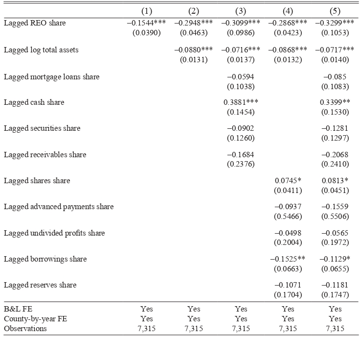
Table 5 presents estimates of the relationship between the lagged share of REO and the share of new loans for a variety of specifications with and without the full set of controls in Equation (1). Specification 1 presents the relationship while including the B&L fixed effects and county-by-year fixed effects, but not other controls. The coefficient is –0.15 and statistically significant at the 1 percent confidence level. When we add controls for lagged log assets, the coefficient increases to –0.29. Adding the remaining balance sheet variables has little impact on the coefficient. In the final step in specification 5, we include the entire range of controls, resulting in a coefficient of –0.33.
BASELINE RESULTS: COEFFICIENT ESTIMATES FOR TIME-VARYING VARIABLES UNDER DIFFERENT SPECIFICATIONS
* = Significant at the 10 percent level in two-tailed t-tests.
** = Significant at the 5 percent level in two-tailed t-tests.
*** = Significant at the 1 percent level in two-tailed t-tests.
Source: The data come from reports of state B&L regulators (see the Appendix).
To understand the magnitude of the coefficient, recall that the mean and the standard deviation of the REO share in Table 4 are 0.08 and 0.14, respectively. Therefore, the estimate from the full specification in Column (5) implies that a one-standard-deviation increase in the REO share is associated with a 4.6-percentage-point decrease (0.140 × –0.329 = –0.046) in the new loans share of total assets in the next period. This is a considerable effect of roughly one-third of the mean of the new loans share in Table 4.
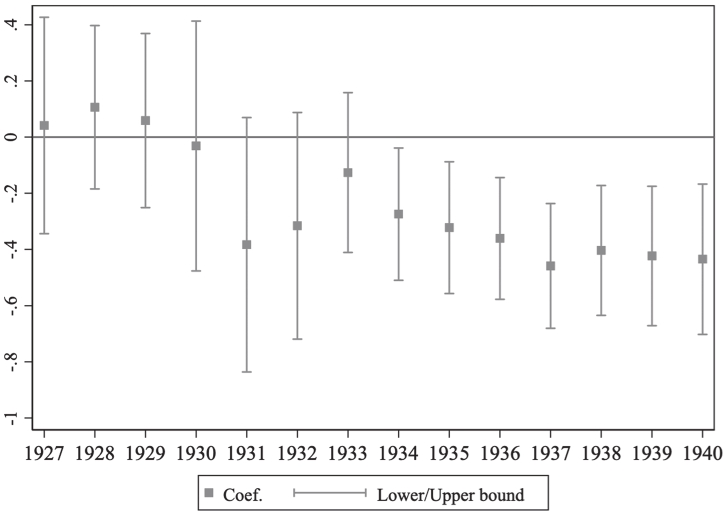
To see how this relationship may have changed over time, we re-estimate the model while allowing the effect of the lagged REO share on new loans to be different each year. Figure 3 presents the point estimates and 95-percent confidence intervals of the year dummies interacted with the lagged REO share, while including all the variables in specification 5 of Table 5. The negative effects of holding REO in the balance sheet begin in 1930 and are negative and statistically different from zero after 1933. The coefficient declines from 1933 to 1937 but not in a statistically significant way. That said, Figure 4 shows the results from multiplying these coefficients with the changes in REO from year to year. The biggest effects come in the mid-1930s when the change in REO was the largest. For comparison, Figure 4 also shows the aggregate change in the new loans as a share of assets each year. At the peak in 1935, the magnitude of the REO effect is about –2 percentage points on the new loans share, at a time when the new loans share increased by about 3 percentage points on average.
EFFECT OF CHANGES IN REO ON NEW LOANS, EVENT STUDY SPECIFICATION
EFFECT OF CHANGES IN REO, MULTIPLIED BY AGGREGATE CHANGE IN REO
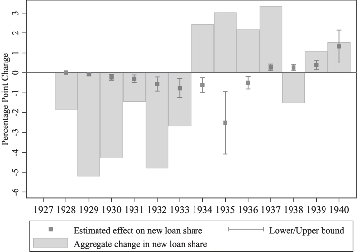
To approximate the impact that the effect of lagged REO share had on the new loans share, we use our results to estimate how much of the change in mean new loans share is explained by the change in mean REO share times the REO coefficient. We do this over two timeframes, 1929–1935 and 1935–1940. The rise of REO between 1929 and 1935 accounts for a larger share of the change in new loans than it does between 1935 and 1940. For the 1929–1935 period, we compute this effect by multiplying the 5.5-percentage-point increase in the mean REO share between 1929 and 1935 by the coefficient estimate (–0.33) and then dividing by the 6.5-percentage-point drop in the new loan share between 1929 and 1935. Thus, the REO channel was associated with approximately 30 percent of the total drop in the mean of new loans during the period. Between 1935 and 1940, the new loan share at the B&Ls increased by 6.6 percentage points, while the mean REO share decreased by only 1 percentage point. After multiplying by the REO coefficient, the reduction in the mean REO share accounted for only 5 percent of the total increase in new loans because the change in the mean REO share was so small.
Overall, the rise in REO over this period acted as a drag on new lending. This drag peaked in the early and mid-1930s as REO climbed rapidly. The recovery in lending, therefore, would have been more robust absent the ongoing drag from greater REO holdings. At the same time, overall lending volumes were also shaped by macroforces, especially including the contraction up to 1933 and re-expansion thereafter.
Our outcome variable is the value of new lending. A common alternative measure of lending in the banking literature is the change in the value of outstanding loans. We examine the differences that arise from using changes in loans as the outcome variable, rather than gross new lending. The correlation between new loans and the change in the loan stock in the sample is a moderate 0.34. Estimating the model with the dependent variable as the change in the loan stock as a percent of assets, instead of the new lending, yields a coefficient on lagged REO changes of –1.8, overestimating the negative effect of REO by a factor of six. This result stems from the fact that increases in foreclosures cause the change in loans to be substantially more negative than the actual number of new loans. These results underscore the importance of using new loans as the outcome variable.
ROBUSTNESS CHECKS
Our estimates can be considered causal under the assumption that the changes in lagged REO within the same B&L over time are uncorrelated with unobserved shocks to their new lending, after accounting for local variation across time in the local housing market captured by county-by-year fixed effects and changes within B&Ls captured by time-varying size, asset structure, and liability structure variables. We now consider an exhaustive set of robustness checks related to this identification strategy. Any subcounty unobservables would have to be of a very particular form and structure to survive all the controls and robustness checks presented below.Footnote 12
Unmeasured B&L Differentiation
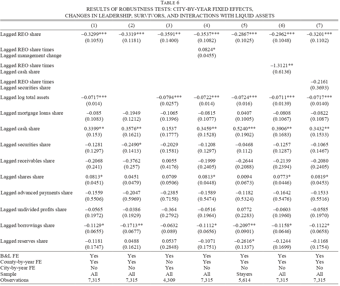
First, we consider robustness to unobserved demand shocks experienced by individual B&Ls. For example, two B&Ls in the same market might serve two different bases of borrowers with different characteristics. One possibility is that B&Ls served different cities within the same county; with this in mind, we estimate our model controlling for city-by-year fixed effects instead of county-by-year effects. The estimated coefficient on lagged REO share is –0.36 using city-by-year fixed effects in Column (3) of Table 6, which is similar to the coefficient of –0.33 from our preferred specification using county-by-year fixed effects (repeated for the sake of convenience in Column (1) of Table 6). Another method is to estimate our main specification using the subsample of B&L in cities in which there is only one B&L operating (35 percent of our main sample) while still controlling for county-by-year fixed effects. Market segmentation inside the same city is not possible in this subsample. Our point estimate for this subsample is –0.33, the same as in the full sample, although it is imprecisely estimated because of the smaller sample size (the standard error is 0.23).Footnote 13
RESULTS OF ROBUSTNESS TESTS: CITY-BY-YEAR FIXED EFFECTS, CHANGES IN LEADERSHIP, SURVIVORS, AND INTERACTIONS WITH LIQUID ASSETS
* = Significant at the 10 percent level in two-tailed t-tests.
** = Significant at the 5 percent level in two-tailed t-tests.
*** = Significant at the 1 percent level in two-tailed t-tests.
Notes: Column (1) repeats the specification reported in Column (5) of Table 5. Column (2) uses city-by-year fixed effects. Column (3) includes only cities with one B&L. Column (4) allows the REO coefficient to differ for B&Ls with changes in management. Column (5) includes only B&Ls that survived to 1940. Columns (6) and (7) interact the lagged REO share with lagged cash and securities shares.
Source: The data come from reports of state and federal B&L regulators (see the Appendix).
Second, we consider the impact of changes in B&L management. In 46 percent of the B&Ls in our sample, at some point during the 1930s, they changed secretaries, the key management figure. We estimate the effect of the lagged REO share while allowing the coefficient to be different for B&Ls with changes in management. In Column (4) of Table 6, the REO coefficient for firms with no secretary change is –0.35, while the effect for those with changes in management is –0.27 (= –0.35 + 0.08) and still statistically significant.
Third, we examine the many B&Ls that failed toward the end of the period. When compared with the surviving B&Ls, it is possible that the firms that failed experienced negative shocks that we have not observed. We estimate the preferred specification for only firms that survived through 1940. In Column (5) of Table 6, the coefficient on REO is –0.29, compared with –0.33 for the results with all firms.
Fourth, we examine whether access to other liquid assets changes the impact of REO. We interact the lagged REO share with the lagged cash share of assets and find little difference in the REO coefficient. The REO coefficient is –0.30 when the lagged cash share is zero and –0.34 when the lagged cash share is at its mean. The coefficient for the interaction between the lags of the REO share and the securities share is statistically insignificant. The REO effect is –0.32 for B&Ls that held no securities and –0.30 for B&Ls with the mean lagged security share.
Finally, we implement the strategy used by Altonji, Elder, and Taber (Reference Altonji, Elder and Taber2015) to evaluate the sensitivity of our results to the potential correlation between the remaining unobservables and both new loans and the REO share. The Altonji, Elder, and Taber (Reference Altonji, Elder and Taber2015) procedure suggests that if the estimates are not sensitive to the inclusion of observables, then they are also unlikely to be driven by the presence of unobservables. To estimate the sensitivity, they compute the ratio of the ordinary least squares (OLS) estimates with covariates as controls divided by the implied bias, which is computed as the OLS estimate with covariates minus the OLS estimate without covariates. This ratio measures how strong the selection on unobservables would have to be, relative to the selection on observables, to explain the entire OLS treatment effect. For the coefficient of –0.33 in the full specification in Column (5) of Table 5, the estimated ratio implies that selection on unobservables would need to be 2 times stronger than selection on observables to reach that value. The lowest ratio measure for any specification in Table 5 is 1.9, and the range of estimates for Table 6 is 1.7 to 3.7.Footnote 14
Government Policy
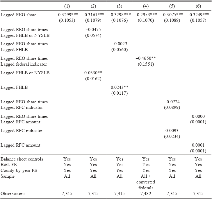
Government policies during the 1930s also might have affected the relationship we find between REO and new lending. First, we consider discounting facilities provided by the New York “S&L Bank” (NYSLB) that existed since 1916 and the FHLB created at the national level in 1932 (Frame, Hancock, and Passmore Reference Frame, Hancock and Passmore2012). These institutions provided discount facilities in which members, who joined voluntarily, obtained loans based on mortgage collateral. We interact the REO share with two dummies, one identifying membership in either or both of these institutions and the second indicating FHLB membership. The coefficients on these interactions are small and not statistically significant (Columns (2) and (3) of Table 7).
ROBUSTNESS CHECKS ASSOCIATED WITH GOVERNMENT POLICIES
* = Significant at the 10 percent level in two-tailed t-tests.
** = Significant at the 5 percent level in two-tailed t-tests.
*** = Significant at the 1 percent level in two-tailed t-tests.
Notes: Column (1) repeats the specification from Column (5) of Table 5. The remaining columns allow the effect of REO to differ by membership in the FHLB system or the NYSLB (Columns (2) and (3)), federal or state charter (Column (4)), and status as a RFC borrower and amount of such lending (Columns (5) and (6)).
Source: The data come from reports of state and federal B&L regulators (see the Appendix).
Second, we consider whether focusing only on state-chartered B&Ls affects the results, insofar as whether those that converted to federal charters had a different experience with REO. We view financial frictions posed by REO as likely to be relevant for federally chartered associations, regardless of the business model changes associated with federal charters.Footnote 15 Column (4) of Table 7 shows the estimates of adding to the sample federal S&Ls that converted from state charters, which account for about 10 percent of state B&Ls, or 20 percent by assets. We also interact the REO coefficient with a federal S&L dummy. The results show that the interaction is highly negative, –0.63, suggesting that, if anything, we have underestimated the effects of REO by excluding a group of low REO firms that converted to federal charters and made a lot of loans. In additional specifications (not reported), we find that if we include all state and federal associations, the coefficient on REO is –0.322, and if we use only state associations that never converted, the coefficient is –0.356. (We also check to see if mergers affect the data, some of which involved federal S&Ls; if we exclude any association involved in a merger, we find a coefficient of –0.34.)
Third, we examine the impact of the RFC, which provided loans to B&Ls and other financial institutions (Calomiris et al. Reference Calomiris, Mason, Weidenmier and Bobroff2013; Vossmeyer Reference Vossmeyer2016). We interact REO with two measures of RFC involvement: a dummy indicating any time after a B&L received an RFC loan and the amount of the RFC loan (equaling zero if no loans were received). Columns (5) and (6) show that the REO measure is relatively unchanged at –0.31 and –0.32.Footnote 16
Finally, we consider how the HOLC’s activities affected the impact of REO. We do not have information regarding B&L-specific HOLC purchases, but we can gain some perspective by comparing year-by-year coefficients before and after the HOLC made the bulk of its loans in 1934 and 1935. Prior to 1931, foreclosure rates were very low and the REO share was low enough that there is only a weak relationship between REO share and new loans. Between 1931 and 1933, the foreclosure crisis spiked and the HOLC had barely started its purchases. Figure 3 shows that the coefficients for 1931–1933 are roughly the same as the coefficients in 1934 and 1935, although the earlier coefficients are imprecisely estimated.Footnote 17 The results suggest that the presence of the HOLC did not significantly alter the relationship between REO and new lending.
Heterogeneity by State and City Size
In our final set of robustness checks, we consider whether heterogeneity across housing markets affects the impact of REO.
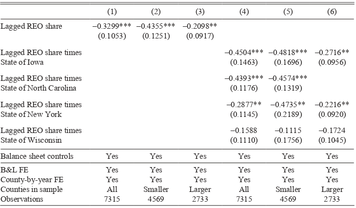
First, we compare small and large markets. Columns (2) and (3) of Table 8 show that when examining subsets of large versus small counties, the coefficient on REO is greater in a specification with only larger-sized counties. The coefficient in the larger-county specification is –0.44 compared to –0.21, though the point estimates are not different from each other with statistical significance. The more negative effects in the smaller counties may be a sign of less liquidity and less depth in the housing markets than in larger markets. Resale of REO likely had stronger negative effects on housing prices, thus further lowering the value of the loan collateral that backed the failed loans. Secondary markets for B&L shares were less likely to develop in smaller counties, and B&Ls in smaller areas likely had smaller networks of potential investors. Courtemanche and Snowden (Reference Courtemanche and Snowden2011) and Fishback et al. (Reference Fishback, Kantor, Flores-Lagunes, Horrace and Treber2011) found substantially larger effects of the HOLC purchase and refinancing of loans on housing prices and home ownership in smaller counties for similar reasons.
HETEROGENEITY OF REO EFFECTS BY STATE AND CITY SIZE
* = Significant at the 10 percent level in two-tailed t-tests.
** = Significant at the 5 percent level in two-tailed t-tests.
*** = Significant at the 1 percent level in two-tailed t-tests.
Notes: Column (1) repeats the specification reported in Column (5) of Table 5. Column (2) includes only B&Ls in small-sized counties, while Column (3) includes those in larger counties. Columns (4)–(6) allow the REO coefficient to differ across states, and the latter two columns restrict the sample to small and large counties.
Source: The data come from reports of state and federal B&L regulators (see the Appendix).
Second, we allow the REO coefficient to differ across states. Housing markets may differ across states for a variety of reasons, including legal frameworks. For example, the foreclosure process took about 16 months to complete in Iowa and Wisconsin, on average, but just a few months in New York and North Carolina (Russell 1937). The REO coefficients for three of the four states in Column (4) of Table 8 are negative and statistically significant. Iowa’s coefficient of –0.44 and North Carolina’s of –0.48 are about a third larger than the overall coefficient of –0.33, while New York’s coefficient of –0.29 is roughly the same. Finally, we also examine how the impact of REO changes across county sizes within each state. Specifications 5 and 6 show that the negative coefficients for smaller counties in New York and Iowa are roughly twice the magnitude of the coefficients in the larger counties. The REO effects in Wisconsin are negative but are smaller and not statistically significant. One reason may be that the sample for Wisconsin starts only in 1935 and, thus, does not cover the peak period of foreclosures that is included in the time frame for the other states.
CONCLUSION
Events since 2007 have reminded us that recessions accompanied by housing crises are unusually severe and protracted. In response, there has been much recent work on the contributory role of financial frictions in these outcomes. For the 1930s episode examined here, we have shown that the supply of credit from the nation’s most important class of mortgage lenders was reduced by frictions caused by foreclosures generated during the crisis. The friction in this case, perhaps better called a clog, was real estate on each B&L’s balance sheet. The real estate that replaced interest-bearing loan assets within these mutual lending organizations generated lower gross returns and imposed higher service and maintenance costs. The combination reduced the pool of loanable funds generated by current assets and cut off new sources of funding by discouraging new B&L investments. For the intermediaries in our four-state sample, a one-standard-deviation increase in the share of assets owned as foreclosed real estate in the prior year lowered the share of assets devoted to new loans by approximately 5 percentage points, or about one-third of the mean share of assets dedicated to new loans during the 1930s. This mechanism accounts for 30 percent of the drop in the mean value of new mortgages issued by these B&Ls between 1929 and 1935. It accounted for much less of the recovery in new lending after 1935 because REO shares changed little, remaining elevated throughout the decade. These empirical results stand up to a broad range of robustness checks and represent evidence that REO on the balance sheet of intermediaries strongly depressed new lending.
Mortgage foreclosures also spiked dramatically during the Great Recession of 2007 and generated similarly low returns and high costs to participants within mortgage lending networks. It is not easy to trace, measure, or estimate the impact of this REO on new lending for the modern era, however, because the impacts are imposed on, and often contested by, multiple participants linked through complex lending networks. The historical context, therefore, offers an unusual and valuable perspective on a mechanism that is less transparent today. B&Ls were the leading institutional residential mortgage lender entering the Great Depression; were exclusively local and residential in lending; and originated, held, and serviced each loan in their portfolio. As equity-financed corporations, and not depository institutions, B&Ls were permitted to continue operation even as REO increased dramatically as a share of assets. These features make the relationship between REO and new lending transparent and measurable for B&Ls of the 1930s. This is especially true for B&Ls in our four-state sample because we have direct information on new loans for each year.
Our results suggest fruitful areas of investigation. In general, the residential finance crisis of the Depression has received far less attention than the crisis in commercial banking. It is important to better understand how the restrictions in B&L lending shown here impacted households and homebuilders. We also need to better understand whether federal policy ameliorated the reduction in credit. Chief among these is the HOLC, which purchased distressed mortgage loans from lenders, including B&Ls, and then refinanced and funded the new loans. More than two million homeowners applied for HOLC refinancing between 1934 and 1936, and the agency accepted one-half of these applications with many of the one million rejected applications ascertained to be “too distressed” to warrant refinancing (Fishback, Rose, and Snowden Reference Fishback, Rose and Snowden2013). Most of these ended up as foreclosed real estate on the balance sheets of B&Ls or other lenders. The analysis here, in this respect, offers a complementary view of the positive impact that HOLC had on homeownership, prices, and building during the 1930s.
The results also suggest some important questions for the modern era. Financial innovation has segmented origination, servicing, and funding, but during a foreclosure crisis, those systems must still absorb the costs and delays associated with the resulting REO. We need to better understand how these costs are distributed and funded within modern lending channels, whether and by how much they choke off new lending, and how policy interventions can be structured to ameliorate these impacts.
Appendix. Data Sources
The data here come from the annual reports of B&L regulators at the state level for Iowa, New York, and North Carolina between 1928 and 1940 and for Wisconsin between 1935 and 1940. In addition, we include federal S&L balance sheet data from 1936 to 1940 in a robustness check. Federal S&L data are not available before 1936. These data were printed in the following sources:
Federal Home Loan Bank Board. Annual Report of Federal Savings and Loan Associations, 1936–1940.
Iowa State Auditor. Report on the Condition of Building and Loan Associations for the Year Ending December 31. Des Moines, IA: State of Iowa, 1928–1940.
New York Superintendent of Banks. Annual Report of the Superintendent of Banks Relative to Savings and Loan Associations, Savings and Loan Bank of the State of New York and Credit Unions for the Year. Albany, NY: J.B. Lyons Company Printers, 1928–1940.
North Carolina Insurance Department. Financial Condition of Building and Loan Associations, 1928–1940.
Wisconsin State Banking Commission. Annual Report on the Condition of Wisconsin Building and Loan Associations and Investment Associations at the Close of Business on December 31. Madison, WI, 1935–1940.
We selected these states because, in addition to including the typical balance sheet information available in other states, the regulators also required B&Ls to report the volume of new lending in these years. Wisconsin’s reports did not include this new lending information before 1935.



