1 Introduction
A ‘bubbly flow’ refers to a multiphase system, where many bubbles are present and influence, in some way, a fluid motion. These flows are involved in a wide range of technological applications, such as gas strippers, direct-contact evaporators and stirred aerated tanks (Ribeiro Jr & Mewes Reference Ribeiro and Mewes2007; Zawala & Malysa Reference Zawala and Malysa2011; Zawala et al. Reference Zawala, Dorbolo, Vandewalle and Malysa2013), which generate a demand for a better understanding of the influence of the bubbles on the flow and the impact of the flow on the bubbles. For example, the collision, bouncing and coalescence of bubbles with liquid/gas and liquid/solid interfaces, as the first and necessary stage for the formation of foams and flotation aggregates (Zawala et al. Reference Zawala, Krasowska, Dabros and Malysa2007), have been the subject of many studies.
The interactions and dynamics of a bubble at liquid/gas and liquid/solid interfaces are well documented. For example, Krzan, Lunkenheimer & Malysa (Reference Krzan, Lunkenheimer and Malysa2003) presented experiments that showed that a bubble approaching an air/water interface can pulsate with a high frequency and rebound. Moreover, Tsao & Koch (Reference Tsao and Koch1997) studied the bouncing when a bubble either interacts with a horizontal rigid wall or rises under an oblique wall. The dynamics of collision was interpreted using an energy balance involving the kinetic energy of the fluid motion, the surface energy of the air/water interface and the gravitational potential energy. Later, Zenit & Legendre (Reference Zenit and Legendre2009) found that the coefficient of restitution, which is defined as the ratio between the rebound and approach velocities of the bubble, can be scaled with the Stokes number, St, and the capillary number, Ca, where St is a dimensionless number that compares the particle inertia with the viscous effects (Gondret, Lance & Petit Reference Gondret, Lance and Petit2002) and Ca represents the relative effect of viscous forces versus surface forces acting on the bubble. Recently, Zawala & Dabros (Reference Zawala and Dabros2013) numerically analysed the energy transfer associated with collision of an air bubble with a solid wall. They quantified the energy dissipation, which is mainly associated with the formation and drainage of the thin liquid film between the colliding bubble and the solid wall, while Klaseboer et al. (Reference Klaseboer, Manica, Hendrix, Ohl and Chan2014) proposed a force-balance model for the bouncing of bubbles at a solid wall, which predicts the time history of the velocity of the bouncing bubble.
Not surprisingly, there is also research on bubble bouncing focused on the influence of different liquid and bubble properties. For example, Sanada, Watanabe & Fukano (Reference Sanada, Watanabe and Fukano2005) experimentally and numerically checked the effect of the liquid viscosity, and they suggested that whether a bubble coalesces with an air/liquid interface or bounces is determined by not only the critical Weber number, We, a dimensionless parameter describing the relative importance of the fluid inertia and surface tension effects, but also the critical Reynolds number, Re, comparing the relative importance of the fluid inertia and viscous effects. Additionally, Suñol & González-Cinca (Reference Suñol and González-Cinca2010) found that for an air/liquid interface, the bouncing time of a bubble increases linearly with We, and the maximum distance from the interface after the first bounce also grows linearly with the bubble equivalent diameter. More recently, Kosior et al. (Reference Kosior, Zawala, Todorov, Exerowa and Malysa2014) investigated the influence of
 $n$
-octanol concentration on the dynamics of a bubble colliding with an air/liquid interface, and documented the bubble coalescence time and stability of the liquid film formed under dynamic conditions. The concentration of
 $n$
-octanol affects the critical rupture thickness of the liquid film: at lower concentrations, the thickness of the rupturing film is a few micrometres, while at higher concentrations, the foam film is able to survive the disturbance caused by the colliding bubble and reaches thicknesses below 100 nm at rupture. In addition, bubble penetration through a liquid/liquid interface (from the lower water phase to the upper oil phase) has also been studied. Uemura, Ueda & Iguchi (Reference Uemura, Ueda and Iguchi2010) observed that the ripples formed by a bubble rising through an immiscible two-liquid interface generate numerous water micro-droplets in the upper oil phase, while Li et al. (Reference Li, Al-Otaibi, Vakarelski and Thoroddsen2014) studied the pinch-off of a small satellite bubble in the water phase when a large bubble penetrates through the oil/water interface.
However, the details of a bubble bouncing at a liquid/liquid/gas interface, which we denote as a compound interface, are much less studied. Recently, Feng et al. (Reference Feng, Roché, Vigolo, Arnaudov, Stoyanov, Gurkov, Tsutsumanova and Stone2014, Reference Feng, Nunes, Shin, Yan, Kong, Prud’homme, Arnaudov, Stoyanov and Stone2016) showed that bubble bursting at an air/oil/water-with-surfactant interface can disperse submicrometre oil droplets into the water column, highlighting the idea that creating a model compound interface may help in better understanding the multiphase physics. In fact, most bubbles formed in nature (e.g. in oceans, lakes, etc.) are coated by an oil layer with a thickness of
 $1{-}100~\unicode[STIX]{x03BC}\text{m}$
because of the ecosystem that is filled with organic materials (Johnson & Cooke Reference Johnson and Cooke1979; Glazman Reference Glazman1983). When two such coated bubbles collide with each other, a compound liquid/liquid/gas interface consisting of air, oil and water is present at the interaction, which will lead to more complex dynamics than the collision of two bare bubbles. In addition, the atmosphere/ocean interface is always covered by the sea surface microlayer, an organic film containing lipids, proteins and hydrocarbons (Cunliffe et al.
Reference Cunliffe, Engel, Frka, Gašparović, Guitart, Murrell, Salter, Stolle, Upstill-Goddard and Wurl2013), which suggests that when a bubble rises to the ocean interface, it interacts with a thin oil layer at the air/water interface. Here, we focus on this scenario, which highlights the effects of a thin oil layer on single-bubble dynamics at the air/water interface. To the best of our knowledge, such effects have rarely been studied.
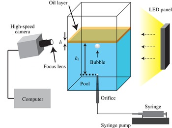
Experimental apparatus. Using a syringe pump, a bubble is generated through a capillary tube fixed at the bottom of the container, and then the bubble approaches the air/oil/water interface because of buoyancy. A computer-controlled high-speed camera is used to observe the bubble motion with lighting provided by an LED panel. The oil layer thickness,
 $h$
, and the distance from the orifice to the oil/water interface,
 $h_{i}$
, are indicated.

In this paper, we add to the understanding of bubble dynamics by reporting an experimental and numerical study of a bubble bouncing at a liquid/liquid/gas interface. The experimental set-up, image analysis and numerical method are presented in § 2. In § 3, we use the experimental observations and the numerical simulations to explore the influence of the oil layer thickness and oil viscosity on the bubble motion and shape deformation. In § 4, we further extend the idea of a reduced-order mass–spring–damper model for the multiphase configuration and test whether it can capture some of the main features of the bubble dynamics. Details of the numerical method are described in appendix A.
2 Experimental set-up and numerical method
2.1 Experimental set-up
The experimental system is shown in figure 1. For each experiment, a thin layer of the dispersed phase, e.g. a non-polar silicone oil (poly(dimethylsiloxane), Sigma-Aldrich), was deposited on deionized water, which was prepared by a purification production unit (
 $\text{resistivity}=18.2~\text{M}\unicode[STIX]{x03A9}~\text{cm}$
, Milli-Q®, Millipore). A bubble was formed at a capillary orifice of inner diameter 0.05–0.10 mm, which was located at the bottom of the tank. A syringe pump (KDS-100, KDS Scientific) was used to precisely control the flow rate of air and hence the bubbling frequency, which was small enough to avoid interface fluctuations caused by impact and rupture of the previous bubble. In addition, the apparatus was placed on an optical table with active isolation legs to further reduce vibrations from the environment. A square acrylic plastic tank, with a cross-section of
 $91\times 91~\text{mm}^{2}$
and a height of 96 mm, was used so that optical distortions could be avoided. The dimensions of the container were much larger than the bubble size and the capillary length in order to minimize the bubble–wall boundary interactions as well as any effects of menisci.
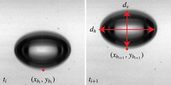
Schematic of the parameters for the image analysis of a rising bubble. The position of the bottom pole of the bubble (
 $x_{b_{i}}$
,
 $y_{b_{i}}$
) in frame
 $i$
is identified. The horizontal and vertical diameters,
 $d_{h}$
and
 $d_{v}$
, are also indicated.

The motion of a bubble was captured by a high-speed video camera (Phantom V7.3, Vision Research) with a frame rate of up to
 $4000~\text{frames}~\text{s}^{-1}$
, an exposure time of 490 or
 $240~\unicode[STIX]{x03BC}\text{s}$
and a spatial resolution of
 $704\times 500$
pixels. A lens (Sigma, DG Macro 105 mm) with bellows was used for obtaining close-up views of a bubble. To avoid the image blur caused by the liquid meniscus on the tank, the camera was placed slightly below the level of the free surface and oriented at an angle of approximately
 $3^{\circ }$
; this tilted set-up reduced the length scale by less than approximately 1 %, so the magnitude of the induced error was negligible (Sato et al.
Reference Sato, Shirota, Sanada and Watanabe2011).
The equivalent diameter of a bubble,
 $d_{eq}$
, defined as a sphere with an identical volume to the distorted bubble which generally has an ellipsoidal shape, was calculated from (Krzan & Malysa Reference Krzan and Malysa2002)
 $$\begin{eqnarray}d_{eq}=(d_{v}d_{h}^{2})^{1/3},\end{eqnarray}$$
where
 $d_{v}$
and
 $d_{h}$
are the vertical and horizontal diameters respectively of the bubble images when the bubble reaches a steady rise velocity, as shown in figure 2. With different inner diameters of the capillary tubes (
 $D=0.05$
, 0.08 and 0.10 mm) used to generate the bubbles in the experiments,
 $d_{eq}$
was determined to be respectively
 $1.30\pm 0.01$
,
 $1.53\pm 0.01$
and
 $1.64\pm 0.01~\text{mm}$
, which are in good agreement with results calculated by Tate’s law (Zawala et al.
Reference Zawala, Krasowska, Dabros and Malysa2007). The thickness of the oil layer,
 $h$
, was estimated using the volume of added oil divided by the cross-sectional area of the container. We neglected the influence of the menisci because of the large cross-sectional area of the oil layer. In the experiments reported here,
 $h=0.75$
, 1, 1.5 and 2 mm. To form a uniform layer of oil at the upper surface of the water bath, more oil was added first and then the extra volume was carefully removed with a syringe. The distance from the orifice to the oil/water interface,
 $h_{i}$
, was controlled to be 9.6, 14.4 and 23.6 mm, which changes the initial approach velocity of the bubble. The distances
 $h$
and
 $h_{i}$
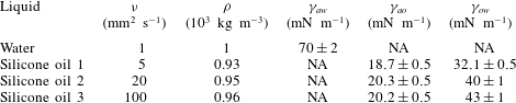
are indicated in figure 1. The physical properties of water and the silicone oils are listed in table 1, and these values were also used in the numerical simulation. The surface tensions of the water and oils and the fluid–fluid interfacial tensions of all phases were measured using the pendant-drop method. We rinsed the container with pure water 10 times before each experiment and covered the container during experiments to avoid the influence of dust. The comparison with literature values for the approach velocity of the bubble (
 $d_{eq}=1.64~\text{mm}$
) released different distances from the oil/water interface (Zawala et al.
Reference Zawala, Krasowska, Dabros and Malysa2007) shows a small maximum absolute relative deviation of 1.9 %, which confirms the purity of the water. The comparison of the bubble shape deformation with literature values will be given later in § 3. The experiments were all carried out at room temperature (
 $25~^{\circ }\text{C}$
). The effect of the heat emitted by the LED panel on the material properties was checked to be negligible.
The physical properties of the working fluids (
 $a$
, air;
 $w$
, water;
 $o$
, oil).

2.2 Image analysis
After capturing the images of a bubble bouncing at the air/oil/water interface, we performed image processing using Matlab routines. When the bubble collides with the interface, a non-uniform background intensity is observed, which interferes with the detection of the bubble shape. Therefore, we subtracted the background before binarizing the image, and then the geometric information of the bouncing bubble was obtained. Values of the bubble velocity in the images,
 $u_{i}$
, were calculated on the basis of the positions in the images with a central difference scheme:
 $$\begin{eqnarray}u_{t_{i}}=\pm \frac{\sqrt{(x_{i+1}-x_{i-1})^{2}+(y_{i+1}-y_{i-1})^{2}}}{t_{i+1}-t_{i-1}},\end{eqnarray}$$
where (
 $x_{i+1},y_{i+1}$
) and (
 $x_{i-1},y_{i-1}$
) are the coordinates of a certain point in the images at times
 $t_{i+1}$
and
 $t_{i-1}$
respectively. An example for the bottom pole of the bubble is shown in figure 2. We define ‘
 $+$
’ as the bubble moving towards the interface. For the results obtained with our experimental set-up, we found that (2.2) is able to capture all of the features compared with higher-order central difference schemes. We also note that in the experimental time range for the first three or four collisions, no horizontal movements were observed. Since the top of the bubble is immersed into the oil layer when the bubble collides with the compound interface, it is difficult to determine directly the bubble centroid and the related velocity. Therefore, we use the velocity of the bubble bottom pole,
 $u_{b}$
, to represent the global dynamics of bouncing, unless otherwise stated. In particular, we apply the velocity of the bubble centroid,
 $u_{c}$
, to describe the parameters related to the kinetic energy associated with the motion of the bubble, such as the coefficient of restitution in §§ 3 and 4. The shape dynamics is indicated by the degree of bubble deformation,
 $\unicode[STIX]{x1D712}$
, which we define as the ratio of the horizontal and vertical diameters of the bubble (figure 2):
 $$\begin{eqnarray}\unicode[STIX]{x1D712}=\frac{d_{h}}{d_{v}}.\end{eqnarray}$$
2.3 Numerical method
Direct numerical simulations are performed using the front-tracking method to examine and gain further insight into the bubble dynamics during the collision and bouncing at the compound interface. The numerical method is described in detail in appendix A. Since in the experiments we do not observe the lateral motion of a bubble before it comes to rest, the flow is assumed to be axisymmetric to facilitate extensive simulations with the high grid resolution required to resolve the water film region between the bubble and the oil layer when the bubble approaches and rebounds. Due to the axisymmetric assumption, the three-dimensional features such as non-vertical collisions, non-symmetrical surface waves and lateral motion of the bubble are not captured in the numerical simulations. In addition, the rupture of the interface is not implemented in the numerical simulations.
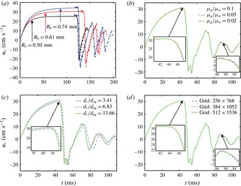
The numerical method is first validated for an air bubble colliding with and bouncing at a simple air/water interface. The results are presented and discussed in appendix B. We find that the numerical results are in good agreement with the experimental data of Zawala et al. (Reference Zawala, Dorbolo, Vandewalle and Malysa2013), especially for the first few collisions (figure 18
a) in appendix B. An extensive study was also performed to demonstrate the grid convergence and examine effects of gas phase viscosity and channel diameter on the bubble dynamics at the compound interface (figure 18
b–d). We find that the effect of the gas phase viscosity is negligible as long as
 $\unicode[STIX]{x1D707}_{g}/\unicode[STIX]{x1D707}_{w}\leqslant 0.1$
(figure 18
b), and there is no significant wall effect when the channel diameter is approximately 6.8 times larger than that of the bubble (figure 18
c), i.e.
 $d_{c}/d_{eq}\geqslant 6.83$
(see the definition of
 $d_{c}$
in figure 17). Thus, the gas phase viscosity is set to
 $\unicode[STIX]{x1D707}_{g}=0.1\unicode[STIX]{x1D707}_{w}$
and the channel diameter is fixed at
 $d_{c}=6.83d_{b}$
or larger in all of the numerical results presented in the current study. For this channel size, the grid convergence is achieved for a
 $256\times 768$
grid (figure 18
d). However, all of the simulations are performed on a much finer grid containing
 $512\times 1536$
grid cells in order to better resolve the water film between the bubble and the oil/water interface during the collision.
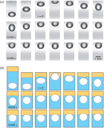
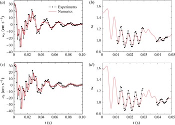
Sequence of (a) experimental and (b) simulation snapshots in a bottom-side view during the collisions of a bubble with a compound interface. Time is set to zero when the top apex of the bubble crosses the undisturbed oil/water interface. The time interval between snapshots is 0.004 s. It should be noted that in the numerical case, the area of observation is enlarged to see the deformation of the oil/water interface. Here,
 $u_{0}=30.6~\text{cm}~\text{s}^{-1}$
,
 $d_{eq}=1.64~\text{mm}$
,
 $\unicode[STIX]{x1D708}_{o}=5~\text{mm}^{2}~\text{s}^{-1}$
,
 $h=2~\text{mm}$
,
 $h_{i}=9.6~\text{mm}$
,
 $Re=5.6\times 10^{2}$
and
 $We=2.2$
.

Comparison of the experimental data (black symbols) and simulation results (red solid lines). (a) Velocity of the bottom pole and (b) shape deformation for
 $d_{eq}=1.64~\text{mm}$
,
 $\unicode[STIX]{x1D708}_{o}=5~\text{mm}^{2}~\text{s}^{-1}$
,
 $h=1~\text{mm}$
,
 $h_{i}=9.6~\text{mm}$
,
 $Re=5.6\times 10^{2}$
and
 $We=2.2$
. (c) Velocity of the bottom pole and (d) shape deformation for
 $d_{eq}=1.64~\text{mm}$
,
 $\unicode[STIX]{x1D708}_{o}=5~\text{mm}^{2}~\text{s}^{-1}$
,
 $h=2~\text{mm}$
,
 $h_{i}=14.4~\text{mm}$
,
 $Re=6.2\times 10^{2}$
and
 $We=2.7$
. It should be noted that
 $\unicode[STIX]{x1D712}$
is not shown when the top part of the bubble is hidden behind the compound interface.

After validation and standard numerical checks, the numerical method is applied to the compound interface case. Individual images of the bubble shape from experiments and simulations are shown in figure 3, which indicates that the experimental and numerical results are in good qualitative agreement. For a more quantitative comparison, the velocity of the bottom pole and the deformation of the bubble are plotted versus time for two typical cases in figure 4. We observe that the numerical simulations capture the translation of the bubble well. For example, the values of the initial approach velocity at
 $t=0$
from the numerical simulations have a maximum absolute relative deviation of 3.8 % compared with the experimental results for all of the cases studied here. The numerical results for
 $\unicode[STIX]{x1D712}$
in figures 4(b) and 4(d) capture the experimentally observed frequency with a slightly smaller amplitude; a possible reason for the small difference may come from the solubility of the oil phase in water.
3 Influence of the oil layer thickness and oil viscosity on the bubble dynamics
To characterize our system and indicate the flow regime, we use four dimensionless parameters, the Morton number (Mo), Eötvös number (Eo), Reynolds number (Re) and Weber number (We), defined as
 $$\begin{eqnarray}\displaystyle Mo & = & \displaystyle \frac{g\unicode[STIX]{x1D707}_{w}^{4}(\unicode[STIX]{x1D70C}_{w}-\unicode[STIX]{x1D70C}_{g})}{\unicode[STIX]{x1D70C}_{w}^{2}\unicode[STIX]{x1D6FE}_{aw}^{3}},\end{eqnarray}$$
 $$\begin{eqnarray}\displaystyle Eo & = & \displaystyle \frac{(\unicode[STIX]{x1D70C}_{w}-\unicode[STIX]{x1D70C}_{g})gd_{eq}^{2}}{\unicode[STIX]{x1D6FE}_{aw}},\end{eqnarray}$$
 $$\begin{eqnarray}\displaystyle Re & = & \displaystyle \frac{\unicode[STIX]{x1D70C}_{w}u_{0}d_{eq}}{\unicode[STIX]{x1D707}_{w}},\end{eqnarray}$$
 $$\begin{eqnarray}\displaystyle We & = & \displaystyle \frac{\unicode[STIX]{x1D70C}_{w}u_{0}^{2}d_{eq}}{\unicode[STIX]{x1D6FE}_{aw}},\end{eqnarray}$$
 $g$
,
 $\unicode[STIX]{x1D707}_{w}$
,
 $\unicode[STIX]{x1D70C}_{w}$
,
 $\unicode[STIX]{x1D70C}_{g}$
(
 $\ll \unicode[STIX]{x1D70C}_{w}$
) and
 $d_{eq}$
are the gravitational acceleration, viscosity of water, density of water and gas and equivalent bubble diameter respectively. The velocity,
 $u_{0}$
, refers to
 $u(t=0)$
, which is the velocity when the top apex of the bubble crosses the undisturbed oil/water interface (see the panels labelled with
 $t=0$
in figure 3). The ranges of the dimensionless parameters are listed in table 2. The bubbles are ellipsoidal just before colliding with the interface without any sign of path instability. Considering our parameter space, the experimental values of
 $\unicode[STIX]{x1D712}$
are compared with a correlation suggested by Legendre, Zenit & Velez-Cordero (Reference Legendre, Zenit and Velez-Cordero2012) for a bubble rising in a pure liquid, i.e.
 $$\begin{eqnarray}\unicode[STIX]{x1D712}=\frac{1}{1-\frac{9}{64}We(1+0.2Mo^{1/10}We)^{-1}}.\end{eqnarray}$$
The maximum absolute relative deviation of
 $\unicode[STIX]{x1D712}$
is only 3.9 % between the experimental results and (3.2), indicating that there is no observable effect of possible contaminants on the bubble deformation. Before considering our experimental system with a compound interface, it will be helpful to revisit the bouncing of a bubble at a single interface. When a bubble rises towards a single interface, the interface deforms and a thin liquid film develops between the bubble and the interface. The pressure in the film further increases, causing film drainage and a force that acts to repel the bubble from the interface. Due to the inertia of the surrounding liquid, the bubble continues to rise and deform. The curvature of the bubble top surface decreases with the film thickness and the velocity of the bubble. This thinning goes on until a film thickness of 10–100 nm is reached (Kosior et al.
Reference Kosior, Zawala, Todorov, Exerowa and Malysa2014). At this separation, the attractive molecular force induces film rupture, and coalescence of the bubble with the interface occurs. If the repelling force stops the motion of the bubble and pushes the bubble away before the film has thinned to the critical thickness, the bubble bounces instead of coalescing, which is the case relevant to the current work.
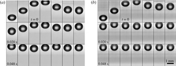
Sequence of snapshots, in a bottom-side view, illustrating collisions of a bubble with (a) an air/water interface and (b) an air/oil/water interface. Time is set to zero when the top apex of the bubble crosses the undisturbed oil/water interface. The time interval between snapshots is 0.004 s. Here,
 $u_{0}=31.6~\text{cm}~\text{s}^{-1}$
,
 $d_{eq}=1.30~\text{mm}$
,
 $\unicode[STIX]{x1D708}_{o}=20~\text{mm}^{2}~\text{s}^{-1}$
,
 $h=1.50~\text{mm}$
,
 $h_{i}=14.4~\text{mm}$
,
 $Re=4.6\times 10^{2}$
and
 $We=1.9$
.

Ranges of the dimensionless parameters in the experimental system.

In order to compare the behaviour of a bubble bouncing at a compound interface versus at an air/water interface, two sequences of experimental snapshots for an air/water and an air/oil/water interface are presented in figure 5. The time interval between successive snapshots is 0.004 s. As shown in figure 5, the bubble first approaches the interface with a nearly constant shape. After the first collision with the interface, the bubble bounces back in the opposite direction to the buoyancy force, while the shape continues to oscillate. The bubble decelerates continuously due to buoyancy and then the second approach begins. Finally, when sufficient energy has been dissipated, the bubble comes to rest beneath the interface. When a compound interface is present, the bouncing amplitudes, translation speeds, degrees of bubble deformation and contact times with the interface are notably different from those with a clean air/water interface. In particular, the bubble bounces less and comes to rest sooner with a compound interface. Additionally, figure 6 shows a top-side view of the experimental snapshots of the interface. For
 $h=2~\text{mm}$
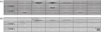
, the amplitude of the top bump is smaller in the presence of a thin oil layer, and only observable during the first collision, while the bump is seen clearly for several collisions for the air/water interface. We note that Gilet & Bush (Reference Gilet and Bush2009) studied a droplet falling onto a horizontal soap film, and found that the deformation of the soap film fits to a catenoid with a constant zero mean curvature beyond the droplet, since the air pressure is atmospheric on either side of the soap film. However, in our case, we do not find that the deformation of either the air/oil or oil/water interface matches a catenoid profile at any time during the collision, since there is a non-zero pressure gradient across these interfaces.
Sequence of snapshots, in a top-side view, of the air/oil interface during the collisions of a bubble with (a) an air/water interface and (b) an air/oil/water interface. Time is set to
 $t_{1}$
when the interfacial deformation is the largest. The time interval between snapshots is 0.004 s. Here,
 $u_{0}=31.6~\text{cm}~\text{s}^{-1}$
,
 $d_{eq}=1.30~\text{mm}$
,
 $\unicode[STIX]{x1D708}_{o}=20~\text{mm}^{2}~\text{s}^{-1}$
,
 $h=1.50~\text{mm}$
,
 $h_{i}=14.4~\text{mm}$
,
 $Re=4.6\times 10^{2}$
and
 $We=1.9$
.

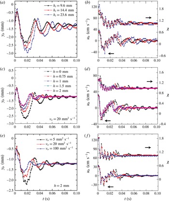
Experimental results. (a) The time evolution of the vertical position of the bubble bottom pole, (b) the velocity of the bubble bottom pole (left
 $Y$
-axis) and the shape deformation of the bubble (right
 $Y$
-axis) for different distances from the orifice to the oil/water interface. Here,
 $d_{eq}=1.64~\text{mm}$
,
 $h=0.75~\text{mm}$
,
 $\unicode[STIX]{x1D708}_{o}=5~\text{mm}^{2}~\text{s}^{-1}$
,
 $Re=5.6{-}6.5\times 10^{2}$
and
 $We=2.2{-}3.0$
. (c) The time evolution of the vertical position of the bubble bottom pole (
 $y_{b}=0$
is denoted as the undisturbed oil/water interface), (d) the velocity of the bubble bottom pole (left
 $Y$
-axis) and the shape deformation of the bubble (right
 $Y$
-axis) for different oil layer thicknesses. Here,
 $d_{eq}=1.30~\text{mm}$
,
 $\unicode[STIX]{x1D708}_{o}=20~\text{mm}^{2}~\text{s}^{-1}$
,
 $h_{i}=23.6~\text{mm}$
,
 $Re=4.8\times 10^{2}$
and
 $We=2.0$
. (e) The time evolution of the vertical position of the bubble bottom pole, (f) the velocity of the bubble bottom pole (left
 $Y$
-axis) and the shape deformation of the bubble (right
 $Y$
-axis) for different oil viscosities. Here,
 $d_{eq}=1.53~\text{mm}$
,
 $h=2~\text{mm}$
,
 $h_{i}=23.6~\text{mm}$
,
 $Re=5.9\times 10^{2}$
and
 $We=2.6$
.

To describe the bubble dynamics, we use the position and velocity of the bubble bottom pole,
 $y_{b}$
and
 $u_{b}$
(figure 7). In addition,
 $\unicode[STIX]{x1D712}$
(2.3) is used to capture the shape dynamics of the bubble. When the top part of the bubble remains hidden at the compound interface, we cannot determine
 $d_{v}$
with our experimental set-up, and so instead we assume a constant volume and calculate the vertical diameter using
 $d_{v}=6V_{b}/(\unicode[STIX]{x03C0}d_{h}^{2})$
, where
 $V_{b}=\unicode[STIX]{x03C0}d_{eq}^{3}/6$
is the volume of the bubble. In our experiments, the oil layer thickness is controlled to be of the same order as the bubble size (see § 2.1). For much thicker oil layers, the influence of the air/oil interface will be lost, and we are interested in the intermediate regime where both the air/oil and oil/water interfaces affect the bubble dynamics.
The time evolutions of
 $y_{b}$
,
 $u_{b}$
and
 $\unicode[STIX]{x1D712}$
in several experimental cases are plotted in figure 7 (see the supplementary materials available at http://dx.doi.org/10.1017/
jfm.2016.517 for all of the experimental data). The approach velocity of the bubble increases with
 $h_{i}$
, as shown in figure 7(a,b). The fluctuation amplitudes of
 $y_{b}$
,
 $u_{b}$
and
 $\unicode[STIX]{x1D712}$
all increase with
 $h_{i}$
due to a larger approach velocity, while the fluctuation frequencies of these parameters remain almost the same. In the following discussion, we focus on the effect of the oil layer on the bubble dynamics. When the oil layer thickness,
 $h$
, increases, the bubble has a smaller maximum bounce distance (figure 7
c), and
 $u_{b}$
decays faster (figure 7
d). This response indicates that the kinetic energy is dissipated faster. Here, we denote the kinetic energy of the bubble as the kinetic energy of the fluid associated with the bubble motion. In figure 7(c), fluctuations at a larger frequency (e.g. see the time window
 $t=0.01{-}0.02~\text{s}$
) are observed since the velocity of the bottom pole is influenced by the bubble shape oscillation (see supplementary movies 1 and 2 for direct observations). In addition,
 $\unicode[STIX]{x1D712}$
is also damped more rapidly with an increase of
 $h$
(figure 7
d). The amplitude between the peak and trough is smaller for larger
 $h$
, which indicates that the surface energy is dissipated faster with a thicker oil layer.
Effects of oil layer thickness from numerical simulations for oil of
 $\unicode[STIX]{x1D708}_{o}=5~\text{mm}^{2}~\text{s}^{-1}$
:
 $h=0.75~\text{mm}$
(left-hand side of each panel) and
 $h=2~\text{mm}$
(right-hand side). Time progresses from (a) to (o), with snapshots taken at
 $t=0$
, 0.001, 0.002, 0.003, 0.004, 0.005, 0.007, 0.009, 0.011, 0.013, 0.015, 0.02, 0.025, 0.03 and 0.035 s. The upper dotted line represents the air/oil interface, while the lower one indicates the oil/water interface. Time is set to zero when the top apex of the bubble crosses the undisturbed oil/water interface. The contours of the constant gauge pressure (Pa) are plotted in the vicinity of the bubble with the legend placed on the right side of each row. Here,
 $u_{0}=30.6~\text{cm}~\text{s}^{-1}$
,
 $d_{eq}=1.64~\text{mm}$
,
 $h_{i}=9.6~\text{mm}$
,
 $Re=5.6\times 10^{2}$
and
 $We=2.2$
.

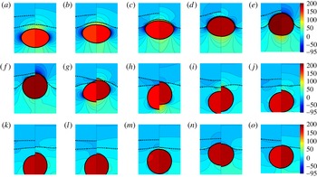
The numerical simulations are utilized to show the whole flow field to obtain more insights. We plot the snapshots from the simulations with pressure distributions for different oil layer thicknesses as shown in figure 8. It should be noted that the pressure value represents the gauge pressure obtained from the absolute pressure minus the atmospheric pressure. When
 $t=0{-}0.004~\text{s}$
, there are no observable differences in the flow field, and the penetration depth is almost the same in the two cases. After
 $t=0.005~\text{s}$
, the air/oil and oil/water interfaces recover faster for a thinner layer, because the restoring force generated by
 $\unicode[STIX]{x1D6FE}_{ow}$
and
 $\unicode[STIX]{x1D6FE}_{ao}$
for a thinner oil layer is larger than that induced mainly by
 $\unicode[STIX]{x1D6FE}_{ow}$
for a very thick oil layer. The bubble also moves back with a larger rebound speed and reaches a deeper depth in the later period when there is a thinner oil layer. On the other hand, to reach the same penetration depth as shown in figure 8, the bubble needs to push up a larger mass of oil for a thicker oil layer. Therefore, the larger mass of the outward oil flow may consume more kinetic energy of the flow. Moreover, the bubble has a longer contact time with the interface when the oil layer is thicker (figure 8), which indicates the possibility to transfer more energy from the bubble to the flow in the oil layer and water film.
Effects of oil layer thickness,
 $h$
, from numerical simulations. (a) The vertical position of the bubble bottom pole,
 $y_{b}$
. (b) The penetration depth,
 $h_{p}$
. (c) The velocity of the bottom pole,
 $u_{b}$
. (d) The shape deformation,
 $\unicode[STIX]{x1D712}$
. Here,
 $d_{eq}=1.64~\text{mm}$
,
 $\unicode[STIX]{x1D708}_{o}=5~\text{mm}^{2}~\text{s}^{-1}$
,
 $h_{i}=23.6~\text{mm}$
,
 $Re=6.5\times 10^{2}$
and
 $We=3.0$
.

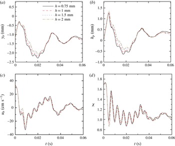
The effect of the oil layer thickness in numerical simulations is summarized in figure 9, where we report the time dependence of various parameters, including the vertical position of the bubble bottom pole,
 $y_{b}$
, the penetration depth
 $h_{p}$
,
 $u_{b}$
and
 $\unicode[STIX]{x1D712}$
. Here,
 $h_{p}$
is defined as the distance between the top apex of the bubble and the undisturbed oil/water interface. In the numerical simulations, we note that the differences for various cases are less significant compared with the experimental trend when
 $h$
changes. The possible reason is that the drainage flow in the water film needs to be better resolved.
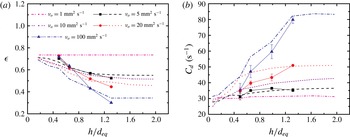
When the oil viscosity increases, the experimental results show a similar trend that
 $y_{b}$
,
 $u_{b}$
and
 $\unicode[STIX]{x1D712}$
approach their final steady values more quickly with a smaller amplitude between the peak and trough for high-viscosity oil (figure 7
e–f). From the energy transfer perspective, at least qualitatively, this result is expected since the increase of the oil viscosity enhances dissipation so that the kinetic energy and surface energy of the bubble are both damped faster.
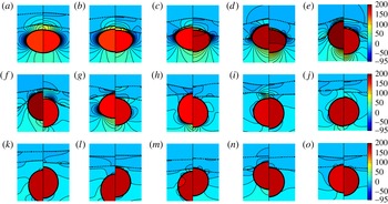
Here, we also plot the snapshots from simulations with the pressure distribution for two cases with different viscosities at the same time side by side as shown in figure 10. For the higher-viscosity oil, the pressures in the water film and the oil layer increase much faster. When
 $t=0.001{-}0.003~\text{s}$
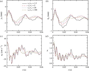
, the maximum pressure in the water film is nearly twice as large when the oil viscosity increases by 20 times. The higher pressure drop induces larger viscous dissipation in the water film, since more energy is consumed for the bubble to push up the oil/water interface and squeeze out the water. The oil layer essentially increases the lubrication force in the water film by effectively changing the top boundary condition of the drainage flow towards no slip. The larger pressure decelerates the bubble in a shorter time, and hence the bubble penetrates less into the oil layer; thus, a bubble interacting with a more viscous oil layer comes to rest sooner. This interpretation of the flow field is consistent with the experimental observations. A summary of the effect of the oil viscosity is shown in figure 11, where a faster damping is observed in all parameters when the oil viscosity increases.
Effects of oil viscosity from numerical simulations:
 $\unicode[STIX]{x1D708}_{o}=5~\text{mm}^{2}~\text{s}^{-1}$
(left-hand side of each panel) and
 $100~\text{mm}^{2}~\text{s}^{-1}$
(right-hand side). Time progresses from (a) to (o), with snapshots taken at
 $t=0$
, 0.001, 0.002, 0.003, 0.004, 0.005, 0.007, 0.009, 0.011, 0.013, 0.015, 0.02, 0.025, 0.03 and 0.035 s. The upper dotted line represents the air/oil interface, while the lower one indicates the oil/water interface. Time is set to zero when the apex of the bubble crosses the undisturbed oil/water interface. The contours of the constant gauge pressure (Pa) are plotted in the vicinity of the bubble with the legend placed on the right side of each row. Here,
 $d_{eq}=1.64~\text{mm}$
,
 $h=0.75~\text{mm}$
,
 $h_{i}=9.6~\text{mm}$
,
 $Re=5.6\times 10^{2}$
and
 $We=2.2$
.

Effects of oil viscosity,
 $\unicode[STIX]{x1D708}_{o}$
, from numerical simulations. (a) The vertical position of the bubble bottom pole,
 $y_{b}$
. (b) The penetration depth,
 $h_{p}$
. (c) The velocity of the bottom pole,
 $u_{b}$
. (d) The shape deformation,
 $\unicode[STIX]{x1D712}$
. Here,
 $d_{eq}=1.64~\text{mm}$
,
 $h=0.75~\text{mm}$
,
 $h_{i}=9.6~\text{mm}$
,
 $Re=5.6\times 10^{2}$
and
 $We=2.2$
.

Next, to obtain a better quantification of the damping effect, we study the velocity change before and after the collision as an indication of the change of the kinetic energy of the bubble. We define the coefficient of restitution, as it is often used to describe bouncing, as
 $$\begin{eqnarray}\unicode[STIX]{x1D716}=-\frac{u_{r}}{u_{i}},\end{eqnarray}$$
where
 $u_{i}$
is the approach velocity of the bubble centroid when the top apex of the bubble crosses the undisturbed oil/water interface at one collision and
 $u_{r}$
is the maximum velocity reached by the bubble centroid when leaving the interface afterwards. The coefficient of restitution is one of the main parameters considered and reported in previous studies of a droplet/bubble colliding with an interface, and it has been widely used to describe the droplet/bubble dynamics in which the effects of the interstitial fluid are important (Tsao & Koch Reference Tsao and Koch1997; Richard & Quéré Reference Richard and Quéré2000; Joseph et al.
Reference Joseph, Zenit, Hunt and Rosenwinkel2001; Legendre, Daniel & Guiraud Reference Legendre, Daniel and Guiraud2005; Gilet & Bush Reference Gilet and Bush2009; Zenit & Legendre Reference Zenit and Legendre2009).
The experimental values of
 $\unicode[STIX]{x1D716}$
for the first collision are presented in figure 12(a). As a reference,
 $\unicode[STIX]{x1D716}\approx 0.8$
for a bubble colliding with an air/water interface in our experiments. For a compound interface with high-viscosity oil and a thicker oil layer,
 $\unicode[STIX]{x1D716}$
can be as small as 0.3, since the dissipation effect increases. In addition, the effect of the oil layer thickness on
 $\unicode[STIX]{x1D716}$
is more prominent for higher-viscosity oil, and the same transition is also captured by the numerical simulations (figure 12
a). We will explain more about this observation at the end of this section.
In order to describe the overall damping evolution, the envelope of the velocity profile can be described as an exponentially decaying function of time if we consider the bubble bouncing behaviour as a damped oscillator. Therefore, we adopt an exponential function
 $u_{b}/u_{0}=A\text{e}^{-C_{d}t}$
to fit the relation between time and the peaks in the velocity profile before the bubble comes to rest at the interface, where
 $A$
and
 $C_{d}$
are coefficients obtained from fitting with a least-squares regression. The coefficient
 $C_{d}$
is considered as a damping rate with dimension
 $(\text{time})^{-1}$
. We found that the coefficients of determination for the fitting are all above 0.80, indicating that the general trend of the velocity decay is captured by an exponential function. The fitting results for
 $C_{d}$
for one typical case of
 $Re=5.9\times 10^{2}$
and
 $We=2.6$
(figure 12
b) verify that the velocity profiles damp faster for a thicker and higher-viscosity oil layer, as expected. Furthermore, there is a transition when the oil viscosity increases, as the influence of
 $h$
is more obvious in both the experimental and the numerical results (figure 12
a). For instance,
 $C_{d}$
remains almost constant with
 $h$
for
 $\unicode[STIX]{x1D708}_{o}=5~\text{mm}^{2}~\text{s}^{-1}$
, while it increases significantly with
 $h$
for
 $\unicode[STIX]{x1D708}_{o}=100~\text{mm}^{2}~\text{s}^{-1}$
. We note that the fitting based on numerical results only involves the first two collisions since the numerical error grows faster at later collisions due to a very thin water film between the bubble and the oil layer.
We interpret the trend of the influence of
 $h$
on
 $C_{d}$
for different values of
 $\unicode[STIX]{x1D708}_{o}$
as follows. We first consider a momentum diffusion length scale
 $\ell _{d}=\sqrt{\unicode[STIX]{x1D708}_{o}T_{c}}$
, where we can estimate
 $\ell _{d}$
using the properties of the oil and the contact time scale,
 $T_{c}$
. The length scale
 $\ell _{d}$
represents the thickness of an oil layer where dissipation is important. For
 $\unicode[STIX]{x1D708}_{o}=5~\text{mm}^{2}~\text{s}^{-1}$
,
 $\ell _{d}/h=0.1{-}0.2$
, while
 $\ell _{d}/h=0.5{-}1.3$
for
 $\unicode[STIX]{x1D708}_{o}=100~\text{mm}^{2}~\text{s}^{-1}$
. When
 $\ell _{d}/h\ll 1$
, the increase of
 $h$
will not significantly affect the amount of oil involved in this dissipation layer. However, when
 $\ell _{d}/h$
is
 $O(1)$
, the added oil still participates in the dissipation and hence the damping from dissipation effects should increase. To validate this hypothesis, in numerical simulations we consider extra cases for a wider range of the parameters, including oil viscosities of 1 and
 $10~\text{mm}^{2}~\text{s}^{-1}$
, and oil layer thicknesses from 0.1 to 3 mm, as shown in figure 12. We have also investigated the scenario for an infinite oil layer, i.e. the top portion of the container is fully filled with the oil phase, but we found that the dynamics changes only slightly and the difference is within the numerical uncertainty when
 $h>3~\text{mm}$
. The minimum value of
 $h$
that induces a change in the bounce mainly depends on the oil viscosity and it is of the order of
 $\ell _{d}$
. Thus, the transition to a plateau occurs at smaller
 $h$
for a less viscous oil, for both
 $\unicode[STIX]{x1D716}$
and
 $C_{d}$
.
(a) The coefficient of restitution,
 $\unicode[STIX]{x1D716}$
, for the first collision and (b) the damping rate,
 $C_{d}$
, regarding different oil layer thicknesses and oil viscosities. The filled symbols are experimental results and the dashed lines are numerical simulations. Here,
 $u_{0}=34.3~\text{cm}~\text{s}^{-1}$
,
 $d_{eq}=1.53~\text{mm}$
,
 $h_{i}=23.6~\text{mm}$
,
 $Re=5.9\times 10^{2}$
and
 $We=2.6$
.

4 Reduced-order mass–spring–damper model
In related complex dynamics problems of a droplet/bubble bouncing on a solid surface, seeking a reduced-order mass–spring–damper analogue is ubiquitous in the literature (Okumura et al. Reference Okumura, Chevy, Richard, Quéré and Clanet2003; Clanet et al. Reference Clanet, Béguin, Richard and Quéré2004; Gilet & Bush Reference Gilet and Bush2009; Sato et al. Reference Sato, Shirota, Sanada and Watanabe2011). This approach has proved useful since surface/interfacial tension often dictates a mechanical restoring force similar to a spring, which indicates that the kinetic energy of the drop or fluid motion associated with the bubble can be stored in deformation during collision. These models are all constructed on the same principle as the mass–spring–damper system where the air/liquid interface is represented by a simple spring. For example, the contact time of the first bounce for a drop on a solid wall was found to be predicted by the half-period of a linear mass–spring model neglecting dissipation (Legendre et al. Reference Legendre, Daniel and Guiraud2005). The addition of the oil layer further complicates the response of the air/oil/water interface, since the properties of the oil layer affect the bubble bouncing dynamics, as shown in the previous discussion. In this section, we are interested in extending the idea of a simple mass–spring–damper system to test whether it can capture and predict the physics of a variety of current experiments without the need for a detailed full-scale numerical simulation. The physical process starts when the bubble surface contacts the compound interface with a thin water film between them.
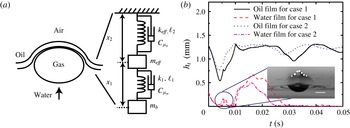
(a) Mass–spring–damper model for a bubble colliding with a compound interface. Here,
 $k$
and
 $\ell$
are respectively the spring constant and the natural length; subscripts 1 and 2 represent the bubble/water and air/oil/water interfaces respectively;
 $k_{eff}$
is the effective spring constant for the compound interface;
 $m_{b}$
is the added mass of the bubble and
 $m_{eff}$
considers the mass of the oil and water layers induced by the bubble collision. The damping effects are considered with
 $C_{\unicode[STIX]{x1D707}_{o}}$
and
 $C_{\unicode[STIX]{x1D707}_{w}}$
. The contribution of gravity to the potential energy is neglected. (b) Time evolution of the oil and water film thicknesses,
 $h_{t}$
, from numerical simulations. Case 1,
 $\unicode[STIX]{x1D708}_{o}=5~\text{mm}^{2}~\text{s}^{-1}$
; case 2,
 $\unicode[STIX]{x1D708}_{o}=20~\text{mm}^{2}~\text{s}^{-1}$
. Here,
 $u_{0}=34.3~\text{cm}~\text{s}^{-1}$
,
 $d_{eq}=1.53~\text{mm}$
,
 $h=1.5~\text{mm}$
,
 $h_{i}=23.6~\text{mm}$
,
 $Re=5.9\times 10^{2}$
and
 $We=2.6$
. Inset: experimental image of the bump at the oil/water interface during the first collision in case 1. The shape of the bump is outlined with a white dashed line. Scale bar: 1 mm.

The essentials of a mass–spring–damper system for a bubble bouncing at a compound interface are shown in figure 13(a). We neglect the gravitational contribution to the change of the potential energy since the vertical positions of the bubble centroid are almost the same when it contacts the compound interface. The deformability of the bubble/water interface is described as a linear spring 1 with a spring constant
 $k_{1}$
that depends on the initial degree of the bubble deformation,
 $\unicode[STIX]{x1D712}$
, right before the bubble collides with the compound interface (Sato et al.
Reference Sato, Shirota, Sanada and Watanabe2011),
 $$\begin{eqnarray}k_{1}=(11.8\unicode[STIX]{x1D712}^{0.6}-1.8)\unicode[STIX]{x1D6FE}_{aw}.\end{eqnarray}$$
Next, we use spring 2 to account for the compound interface. With the oil layer at the interface, we have a compound air/oil/water interface that may behave as an interface with an effective interfacial tension, which can be a complicated nonlinear and time-dependent function of
 $\unicode[STIX]{x1D6FE}_{ao}$
,
 $\unicode[STIX]{x1D6FE}_{ow}$
and other physical parameters of the oil layer; these features make a direct extension of the model of Sato et al. (Reference Sato, Shirota, Sanada and Watanabe2011) non-trivial. Nonetheless, we will seek a low-order expression for the effective interfacial tension and see whether the model can capture some features of the experiments.
We can gain insights by considering the limit of a very thin oil layer. With typical values of the interfacial tensions, we expect that the deformations of both the air/oil and the oil/water interfaces should be approximately comparable, and therefore the effective interfacial tension should scale linearly with each surface tension. Thus, we propose an effective spring constant as
 $$\begin{eqnarray}k_{eff}=A(\unicode[STIX]{x1D6FE}_{ow}+\unicode[STIX]{x1D6FE}_{ao}),\end{eqnarray}$$
where
 $A$
is a constant fitted by the experimental data. Furthermore, the added mass of the bubble,
 $m_{b}$
, as shown in figure 13, is calculated as (Zawala et al.
Reference Zawala, Krasowska, Dabros and Malysa2007)
 $$\begin{eqnarray}m_{b}=C_{m}\unicode[STIX]{x1D70C}_{w}V_{b}\quad \text{and}\quad C_{m}=\frac{\unicode[STIX]{x1D6FC}}{2-\unicode[STIX]{x1D6FC}},\end{eqnarray}$$
where
 $$\begin{eqnarray}\unicode[STIX]{x1D6FC}=\frac{2\unicode[STIX]{x1D712}^{2}}{\unicode[STIX]{x1D712}^{2}-1}\left(1-\frac{1}{\sqrt{\unicode[STIX]{x1D712}^{2}-1}}\cos ^{-1}\left(\frac{1}{\unicode[STIX]{x1D712}}\right)\right).\end{eqnarray}$$
Here, we estimate
 $C_{m}$
using the bubble shape deformation
 $\unicode[STIX]{x1D712}$
at
 $t=0$
and assume that the bubble rises in an unbounded liquid. We note that there is some influence of the interface on the added mass of the bubble. For the case of a bubble approaching a no-slip solid wall,
 $C_{m}$
changes with the distance between the bubble and the interface while maintaining the same order of magnitude (Zawala & Dabros Reference Zawala and Dabros2013). When a bubble approaches a slip and deformable air/oil/water interface in the current experiments, we anticipate that
 $C_{m}$
does not change significantly, and the influence of the distance from the interface on
 $C_{m}$
is neglected.
Furthermore,
 $m_{eff}$
in figure 13(a) takes into account the effective mass of the oil and water layers. The effective mass of the oil,
 $m_{o}$
, pushed away by the bubble, is likely to be time-dependent and also a nonlinear function of other physical parameters in the system. We can gain insights by considering a very thin oil layer, where the effective oil mass for all of our experiments can be estimated as
 $m_{o}=\unicode[STIX]{x1D70C}_{o}\unicode[STIX]{x03C0}(d_{eq}/2)^{2}h$
. Since the bubble continuously deforms when it contacts the interface, we use
 $d_{eq}$
(2.1) as an average horizontal length scale to describe the mean effective oil mass pushed up, rather than
 $d_{h}$
in the period when the bubble collides with the interface.
To gain more insights into
 $m_{w}$
and
 $m_{o}$
, we obtain from numerical simulations the evolution of the thicknesses at the bubble centreline,
 $h_{t}$
, for the oil and water films, as shown in figure 13(b). Typically, both the oil and the water films get thinner as the bubble approaches the oil/water interface, and the water film thickness reaches a minimum value of
 $O(0.1)~\text{mm}$
, although this time dependence is not considered in the current model. Regarding the magnitude of
 $m_{w}$
, the thickness of the water film is much smaller than the oil layer thickness during collision (figure 13
b), and hence we neglect the mass of the water film, i.e.
 $m_{eff}=m_{o}+m_{w}\approx m_{o}$
. Furthermore, we note that at
 $t\approx 0.005{-}0.007~\text{s}$
, a sudden jump occurs in the thickness profiles, which indicates a bump at the oil/water interface, as confirmed by the experimental image (inset of figure 13
b). We attribute this feature to the capillary waves converging towards the centreline (Blanchette & Bigioni Reference Blanchette and Bigioni2006).
For the damping coefficient
 $C_{\unicode[STIX]{x1D707}_{w}}$
of spring 1, we model the viscous force generated in the water film (Zenit & Legendre Reference Zenit and Legendre2009). For a clean bubble approaching a solid wall in a surrounding fluid, the resulting lubrication force is
 $F_{lub}=(3/2)\unicode[STIX]{x03C0}\unicode[STIX]{x1D707}_{w}(d/2)^{2}u/h_{gap}$
, where
 $u$
is the velocity of the sphere,
 $d$
is the sphere diameter and
 $h_{gap}$
is the gap between the solid sphere and the solid wall. Although we have a clean and deformable bubble impacting with an air/oil/water interface, since
 $\unicode[STIX]{x1D707}_{o}>\unicode[STIX]{x1D707}_{w}$
, the viscous oil layer effectively changes the top boundary condition of the drainage flow in the water film towards no slip. We still assume the above expression to estimate the viscous force in the water film. It was found that
 $h_{gap}\sim (d/2)Ca^{1/2}$
(Legendre et al.
Reference Legendre, Daniel and Guiraud2005). Therefore,
 $C_{\unicode[STIX]{x1D707}_{w}}=(3/4)\unicode[STIX]{x03C0}\unicode[STIX]{x1D707}_{w}d_{eq}Ca^{-1/2}$
. Considering the damping in the oil layer, we propose that
 $C_{\unicode[STIX]{x1D707}_{o}}=B\unicode[STIX]{x1D707}_{o}h$
by dimensional arguments and
 $B$
is a coefficient fitted by the experiments. We note that we only focus on the characterization of the collision–rebound process when the bubble interacts with the compound interface. Therefore, the damping effects in the mass–spring–damper model are different from the overall damping rate
 $C_{d}$
in figure 12(b), which also involves damping effects when the bubble moves away from the interface.
Additionally, with the current size range, the bubble is deformed before collision; thus, the initial bubble deformation is described as the initial deformation,
 $x_{1}^{\prime }$
, for spring 1 at the starting point. In figure 13,
 $\ell _{1,2}$
denote the natural lengths of springs 1 and 2 respectively, while
 $x_{1,2}$
are the instantaneous lengths. The dynamic equations of the mass–spring–damper system are written as
 $$\begin{eqnarray}\displaystyle & \displaystyle m_{eff}\frac{\text{d}^{2}x_{2}}{dt^{2}}=-k_{eff}(x_{2}-\ell _{2})-C_{\unicode[STIX]{x1D707}_{o}}\frac{\text{d}x_{2}}{\text{d}t}+k_{1}(x_{1}-x_{1}^{\prime }-\ell _{1}) & \displaystyle \nonumber\\ \displaystyle & \displaystyle +\,C_{\unicode[STIX]{x1D707}_{w}}\left(\frac{\text{d}(x_{1}+x_{2})}{\text{d}t}-\frac{\text{d}x_{2}}{\text{d}t}\right),\hspace{5.0pt} & \displaystyle\end{eqnarray}$$
 $$\begin{eqnarray}\displaystyle & \displaystyle m_{b}\frac{\text{d}^{2}(x_{1}+x_{2})}{\text{d}t^{2}}=-k_{1}(x_{1}-x_{1}^{\prime }-\ell _{1})-C_{\unicode[STIX]{x1D707}_{w}}\left(\frac{\text{d}(x_{1}+x_{2})}{\text{d}t}-\frac{\text{d}x_{2}}{\text{d}t}\right). & \displaystyle\end{eqnarray}$$
 $$\begin{eqnarray}D_{1}=(x_{1}+x_{2})-(\ell _{1}+\ell _{2}+x_{1}^{\prime })\quad \text{and}\quad D_{2}=x_{2}-\ell _{2},\end{eqnarray}$$
where
 $D_{i}$
denotes the deformation of the bubble/water and compound interfaces with subscripts
 $i=1$
and 2 respectively. Then, we obtain
 $$\begin{eqnarray}\displaystyle m_{eff}\frac{\text{d}^{2}D_{2}}{\text{d}t^{2}} & = & \displaystyle -k_{eff}D_{2}-C_{\unicode[STIX]{x1D707}_{o}}\frac{\text{d}D_{2}}{\text{d}t}+k_{1}(D_{1}-D_{2})+C_{\unicode[STIX]{x1D707}_{w}}\left(\frac{\text{d}D_{1}}{\text{d}t}-\frac{\text{d}D_{2}}{\text{d}t}\right),\end{eqnarray}$$
 $$\begin{eqnarray}\displaystyle m_{b}\frac{\text{d}^{2}D_{1}}{\text{d}t^{2}} & = & \displaystyle -k_{1}(D_{1}-D_{2})-C_{\unicode[STIX]{x1D707}_{w}}\left(\frac{\text{d}D_{1}}{\text{d}t}-\frac{\text{d}D_{2}}{\text{d}t}\right).\end{eqnarray}$$
Now, we non-dimensionalize (4.7) considering
 $\tilde{D}_{i}=D_{i}/d_{eq}$
and
 $\tilde{t}=tu_{0}/d_{eq}$
. Dropping the ‘
 $\tilde{~}$
’ symbol, we obtain
 $$\begin{eqnarray}\displaystyle & \displaystyle \frac{\text{d}^{2}D_{2}}{\text{d}t^{2}}+\frac{\unicode[STIX]{x1D705}_{2}}{R\text{e}_{o}^{\ast }}\frac{\text{d}D_{2}}{\text{d}t}+\frac{\unicode[STIX]{x1D705}_{1}}{W\text{e}_{o1}^{\ast }}D_{2}-\frac{\unicode[STIX]{x1D705}_{4}}{R\text{e}_{ow}^{\ast }Ca^{1/2}}\frac{\text{d}(D_{1}-D_{2})}{\text{d}t}-\frac{\unicode[STIX]{x1D705}_{3}}{W\text{e}_{o2}^{\ast }}(D_{1}-D_{2})=0,\quad & \displaystyle\end{eqnarray}$$
 $$\begin{eqnarray}\displaystyle & \displaystyle \frac{\text{d}^{2}D_{1}}{\text{d}t^{2}}+\frac{\unicode[STIX]{x1D705}_{6}}{R\text{e}_{b}^{\ast }Ca^{1/2}}\frac{\text{d}(D_{1}-D_{2})}{\text{d}t}+\frac{\unicode[STIX]{x1D705}_{5}}{W\text{e}_{w}^{\ast }}(D_{1}-D_{2})=0, & \displaystyle\end{eqnarray}$$
 $$\begin{eqnarray}\displaystyle \left.\begin{array}{@{}c@{}}\displaystyle We_{o1}^{\ast }=\frac{\unicode[STIX]{x1D70C}_{o}hu_{0}^{2}}{k_{eff}},\quad We_{o2}^{\ast }=\frac{\unicode[STIX]{x1D70C}_{o}hu_{0}^{2}}{k_{1}},\quad Re_{o}^{\ast }=\frac{\unicode[STIX]{x1D70C}_{o}d_{eq}u_{0}}{\unicode[STIX]{x1D707}_{o}},\quad Re_{ow}^{\ast }=\frac{\unicode[STIX]{x1D70C}_{o}hu_{0}}{\unicode[STIX]{x1D707}_{w}},\\ \displaystyle Ca=\frac{\unicode[STIX]{x1D707}_{w}u_{0}}{\unicode[STIX]{x1D6FE}_{aw}},\quad We_{w}^{\ast }=\frac{C_{m}\unicode[STIX]{x1D70C}_{w}d_{eq}u_{0}^{2}}{k_{1}}\quad \text{and}\quad Re_{b}^{\ast }=\frac{C_{m}\unicode[STIX]{x1D70C}_{w}d_{eq}u_{0}}{\unicode[STIX]{x1D707}_{w}}.\end{array}\right\}\quad & & \displaystyle\end{eqnarray}$$
Here,
 $\unicode[STIX]{x1D705}_{i}$
absorb all of the numerical constants, and they can be estimated for each experiment under the model assumptions. Multiple non-dimensional parameters here are influenced by the properties of both water and oil. We numerically solve (4.8) using the fourth-order Runge–Kutta method, subject to the initial conditions
 $D_{1}(t=0)=0,(\text{d}D_{1}/\text{d}t)(t=0)=-1,D_{2}(t=0)=0,(\text{d}D_{2}/\text{d}t)(t=0)=0$
, where
 $A=7.0$
and
 $B=7.1$
. Below, we focus on the time of contact with the compound interface and the coefficient of restitution, since these are commonly used to describe the rebound of a droplet/bubble (Legendre et al.
Reference Legendre, Daniel and Guiraud2005).
4.1 Bubble–interface contact time
The rebound of a bubble from an interface is characterized by a very short contact time. Whether a bubble can bounce or coalesce during one collision depends on the comparison of the contact time and the drainage time of the liquid film formed between the bubble and the interface. If the contact time is longer than the drainage time and the film is thin enough for molecular-scale (e.g. van der Waals) interactions to act, then the bubble coalesces during the collision. Here, we define the contact time to begin when the top apex of a bubble crosses the undisturbed oil/water interface and to end when the top apex crosses that interface again (Sato et al. Reference Sato, Shirota, Sanada and Watanabe2011).
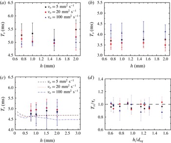
The effects of the oil layer thickness and oil viscosity on the shape oscillation period of the bubble: (a)
 $d_{eq}=1.64~\text{mm}$
, (b)
 $d_{eq}=1.30~\text{mm}$
, (c)
 $d_{eq}=1.53~\text{mm}$
. The filled symbols are experimental results and the dashed lines are numerical simulations. Here,
 $h_{i}=23.6~\text{mm}$
in (a–c). (d) Normalized shape oscillation period,
 $T_{s}/\unicode[STIX]{x1D70F}_{s}$
as a function of
 $h/d_{eq}$
for different oil viscosities and bubble diameters. The theoretical value
 $\unicode[STIX]{x1D70F}_{s}$
is given by (4.10).

The study of Duineveld (Reference Duineveld1994) stated that the contact time of two bubbles in pure water is of the same order of magnitude as the characteristic period of the shape oscillation for a bubble in an unbounded fluid, which is given by Lamb (Reference Lamb1945). The second mode of the Lamb oscillation,
 $\unicode[STIX]{x1D70F}_{s}$
, is related to the bubble shape, which can be calculated using
 $\unicode[STIX]{x1D6FE}_{aw},\unicode[STIX]{x1D70C}_{w}$
and
 $d_{eq}$
(Lamb Reference Lamb1945) as
 $$\begin{eqnarray}\unicode[STIX]{x1D70F}_{s}=\frac{\unicode[STIX]{x03C0}}{2}\sqrt{\frac{\unicode[STIX]{x1D70C}_{w}d_{eq}^{3}}{6\unicode[STIX]{x1D6FE}_{aw}}}.\end{eqnarray}$$
In our system the bubble shape oscillates near a compound interface, so the liquid is no longer unbounded. However, from the experiments, the period of the bubble shape oscillations,
 $T_{s}$
, measured by checking the fluctuations of the bubble surface area when the bubble first moves away from the interface and before the second collision, shows that the oil viscosity and layer thickness do not play a significant role influencing the shape oscillation period (figure 14
a–c). The comparison with the numerical simulations in figure 14(c) also confirms this observation. Furthermore, normalizing
 $T_{s}$
by the theoretical prediction of (4.10),
 $\unicode[STIX]{x1D70F}_{s}$
, collapses the data for multiple cases, as shown in figure 14(d). A similar observation for experiments with an air/water interface was made by Suñol & González-Cinca (Reference Suñol and González-Cinca2010), who found that the bubble oscillation frequency is not affected by the existence of a free air/water surface. When the bubble almost rests at the interface, the bubble shape still oscillates slightly; however, the oil layer blocks observations of the top part of the bubble and also our image resolution is not high enough to detect the small shape oscillations.
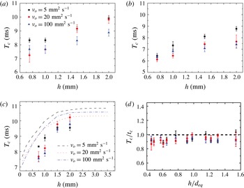
Contact time of the first collision for various bubble diameters: (a)
 $d_{eq}=1.64~\text{mm}$
, (b)
 $d_{eq}=1.30~\text{mm}$
, (c)
 $d_{eq}=1.53~\text{mm}$
for different oil layer thicknesses and oil viscosities. The filled symbols are experimental results and the dashed lines are numerical simulations. Here,
 $h_{i}=23.6~\text{mm}$
in (a–c). (d) Dimensionless contact time of the first collision, with the predicted value as a function of the normalized oil layer thickness. The theoretical value,
 $t_{c}$
, is given by the numerical solution of (4.8) (see § 4.1 for details).

Nevertheless, unlike the statement made by Duineveld (Reference Duineveld1994) for bubble–bubble interactions, we find that the contact time cannot simply be formulated as (4.10). We focus on cases where
 $h_{i}$
is the largest; the impact velocity and the degree of bubble deformation have almost reached their steady values before the bubble collides with the interface. The measured contact times of the first collision,
 $T_{c}$
, for all of the experimental cases are plotted in figure 15(a–c). For the measurements, we used
 $4000~\text{frames}~\text{s}^{-1}$
to ensure that the uncertainty in the experimental observation was less than 4 %. However, the absolute relative deviations between the experimental contact time and the estimation using (4.10) are approximately 30 %–60 %. Therefore, it is difficult to predict the contact time with the use of the shape oscillation mode of the bubble, since it does not take into account the contribution from the deformable compound interface and the oil layer. We also performed numerical simulations for a larger range of oil layer thicknesses from 0.1 to 3 mm, as shown in figure 15(c), which covers more cases than the experiments. The numerical calculations capture a similar trend to the experiments, and reveal that
 $T_{c}$
approaches a plateau when
 $h$
is large. Such a trend is consistent with the results shown in figure 12.
After solving for the time evolution of
 $D_{1}$
from (4.8), we define
 $t_{c}$
as the period when the value of
 $D_{1}$
first becomes 0 again after
 $t=0$
. When we scale
 $T_{c}$
with the predicted value,
 $t_{c}$
, all data points collapse, and the mean absolute relative deviation of all data is
 $7\pm 3\,\%$
, as shown in figure 15(d), indicating that the trend in the current experimental cases is captured by the mass–spring–damper model proposed here. The results show that when we have a compound interface, the contact time of the bubble with the interface will be prolonged compared with the case with an air/water interface (Sato et al.
Reference Sato, Shirota, Sanada and Watanabe2011). When we increase the thickness of the oil layer
 $h$
from 0,
 $m_{eff}$
increases and so does the contact time. If
 $h$
is much larger than the order of
 $\ell _{d}$
, increase of
 $h$
will not significantly influence
 $m_{eff}$
and thus the contact time, as we have discussed in § 3. We note that the contact time increases with the time of bouncing, but after the first bounce, the bubble oscillates significantly, and capillary waves formed on the oil/water and air/oil interfaces propagate away. The energy loss due to these motions has not been considered in the model, and hence the contact time of the second or third bounce cannot be predicted well.
4.2 Coefficient of restitution
From the numerical solution of (4.8), we obtain the theoretical prediction of
 $\unicode[STIX]{x1D716}$
as
 $$\begin{eqnarray}\unicode[STIX]{x1D716}_{t_{c}}=-\frac{\displaystyle \left.\frac{\text{d}D_{1}}{\text{d}t}\right|_{t=t_{c}}}{\displaystyle \left.\frac{\text{d}D_{1}}{\text{d}t}\right|_{t=0}}=\left.\frac{\text{d}D_{1}}{\text{d}t}\right|_{t=t_{c}}.\end{eqnarray}$$
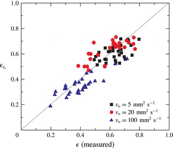
For dozens of experimental cases with different bubble diameters, oil layer thicknesses and approach velocities, the comparison with the measured
 $\unicode[STIX]{x1D716}$
is shown in figure 16. The model seems to capture parts of the main experimental trends, but does not describe all of the complexity for the three types of oil. Although a mass–spring–damper model works well in many cases of a droplet/bubble bouncing at an interface, the addition of the oil layer introduces complications. Given the simplicity of the mass–spring–damper model, we believe that it serves as a useful complement to the full-scale direct numerical simulation approach.
Theoretical prediction from the numerical solution of (4.8),
 $\unicode[STIX]{x1D716}_{t_{c}}$
, versus the measured coefficient of restitution,
 $\unicode[STIX]{x1D716}$
, from the experiments. The solid line represents agreement between the experiments and predictions.

5 Summary
Here, we investigate how an air/water interface coated by a thin oil layer influences the dynamics of bubble bouncing. Such a multiphase configuration is inspired by our previous study on how nanoemulsions can be formed when a bubble bursts at a compound interface (Feng et al. Reference Feng, Roché, Vigolo, Arnaudov, Stoyanov, Gurkov, Tsutsumanova and Stone2014, Reference Feng, Nunes, Shin, Yan, Kong, Prud’homme, Arnaudov, Stoyanov and Stone2016). The air/oil/water compound interface quantitatively changes the bubble motion, since the oil layer acts like a damper and an energy sink for the dynamics of the bubble. To fully understand the modified dynamics, we study the effects of the oil viscosity and oil layer thickness by quantifying the time evolution of the velocity of the bottom pole of the bubble and the shape deformation. The time evolution of these two parameters decays faster with increases of the oil viscosity and layer thickness. With numerical simulations, we also show that the oil viscosity and layer thickness affect the detailed flow field inside the oil layer and water film and hence the energy transfer during impact. The results suggest that the oil viscosity mainly influences the pressure in the water film and hence the drainage flow between the oil layer and the bubble. Higher oil viscosity contributes to a more significant dissipation effect in the water film. The effect of the oil layer thickness may come from the mass of the oil being pushed away by the bubble, which increases with a larger layer thickness.
Additionally, we quantify the damping effects by investigating the coefficient of restitution and the temporal evolution of the bubble velocity profile. The damping coefficients indicate a different trend with the oil layer thickness when the oil viscosity changes. We interpret this as the effect of different ratios between a momentum diffusion length scale controlled by the oil viscosity and the actual oil layer thickness.
We further tested the idea of a reduced-order mass–spring–damper model to describe the bounce of a droplet/bubble at a compound interface and focused on the prediction of the contact time and coefficient of restitution. The deformability of the compound interface was described with an effective surface tension. For the current experiments, the period of the bubble shape oscillations was not the same as the contact time. Instead, the mass–spring–damper model was found to capture the contact time of the first impact quite well. In addition, the experimental trends for the coefficient of restitution were also reasonably predicted by the model, but not all of the complexity in the multiphase system is captured by such a low-order model.
The current study contributes to the understanding of a bubbly flow where such a liquid/liquid/gas interface is present. In fact, most multiphase fluid systems contain surfactants, which are typically present as contaminants, impurities or additives. Hence, a potential future study would include the effect of surfactants, which induce Marangoni stresses at the interface. A systematic analysis of how surfactants affect the flow field would reveal more of the underlying physics for the effect of a compound interface on bubble dynamics.
Acknowledgements
J.F. and H.A.S. thank Unilever Research for support of the research, and L. N. Arnaudov and S. D. Stoyanov for helpful conversations. M.M. acknowledges the support of the Scientific and Technical Research Council of Turkey (TUBITAK), Grant no. 112M181 and by the COST Action MP1106. This work began when M.M. was a visitor at the Department of Mechanical and Aerospace Engineering at Princeton University.
Supplementary material and movies
Supplementary material and movies are available at http://dx.doi.org/10.1017/jfm. 2016.517.
Appendix A. Formulation of the numerical method
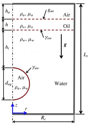
The flow equations are solved within the finite-difference/front-tracking (FD/FT) framework. The flow is assumed to be incompressible and symmetric about the
 $z$
-axis, as sketched in figure 17. The gas and liquid phases are Newtonian fluids with different material properties. Following Unverdi & Tryggvason (Reference Unverdi and Tryggvason1992), a single set of governing equations can be written for the entire computational domain, using the conservative form of the flow equations to allow the material properties to vary discontinuously across the interfaces. Surface tension is added to the momentum equations using delta functions to provide the proper interface boundary conditions.
Schematic illustration of the computational set-up. A spherical bubble of diameter
 $d_{eq}$
is instantly placed on the channel centreline with the initial distance between the bottom pole of the bubble and the oil/water interface,
 $h_{i}$
. The undisturbed oil and air layers have thicknesses
 $h$
and
 $h_{a}$
respectively. The cylindrical channel has a diameter of
 $d_{c}=2R_{c}$
and a length of
 $L_{c}$
.

In a cylindrical coordinate system and assuming axisymmetry, the Navier–Stokes equations can be written as
 $$\begin{eqnarray}\displaystyle & & \displaystyle \frac{\unicode[STIX]{x2202}(\unicode[STIX]{x1D70C}v_{r})}{\unicode[STIX]{x2202}t}+\frac{1}{r}\frac{\unicode[STIX]{x2202}(r\unicode[STIX]{x1D70C}v_{r}^{2})}{\unicode[STIX]{x2202}r}+\frac{\unicode[STIX]{x2202}(\unicode[STIX]{x1D70C}v_{r}v_{z})}{\unicode[STIX]{x2202}z}=-\frac{\unicode[STIX]{x2202}p}{\unicode[STIX]{x2202}r}+\frac{\unicode[STIX]{x2202}}{\unicode[STIX]{x2202}r}\left(2\unicode[STIX]{x1D707}\frac{\unicode[STIX]{x2202}v_{r}}{\unicode[STIX]{x2202}r}\right)+\frac{\unicode[STIX]{x2202}}{\unicode[STIX]{x2202}r}\left(2\unicode[STIX]{x1D707}\frac{v_{r}}{r}\right)\nonumber\\ \displaystyle & & \displaystyle \qquad +\,\frac{\unicode[STIX]{x2202}}{\unicode[STIX]{x2202}z}\left(\unicode[STIX]{x1D707}\left(\frac{\unicode[STIX]{x2202}v_{z}}{\unicode[STIX]{x2202}r}+\frac{\unicode[STIX]{x2202}v_{r}}{\unicode[STIX]{x2202}z}\right)\right)-\int _{A}\unicode[STIX]{x1D6FE}\unicode[STIX]{x1D705}\boldsymbol{n}\unicode[STIX]{x1D6FF}(\boldsymbol{x}-\boldsymbol{x}_{f})\,\text{d}\boldsymbol{A}\boldsymbol{\cdot }\hat{\boldsymbol{i}}_{r},\end{eqnarray}$$
 $$\begin{eqnarray}\displaystyle & & \displaystyle \frac{\unicode[STIX]{x2202}(\unicode[STIX]{x1D70C}v_{z})}{\unicode[STIX]{x2202}t}+\frac{1}{r}\frac{\unicode[STIX]{x2202}(r\unicode[STIX]{x1D70C}v_{r}v_{z})}{\unicode[STIX]{x2202}r}+\frac{\unicode[STIX]{x2202}(\unicode[STIX]{x1D70C}v_{z}^{2})}{\unicode[STIX]{x2202}z}=-\frac{\unicode[STIX]{x2202}p}{\unicode[STIX]{x2202}z}+\frac{1}{r}\frac{\unicode[STIX]{x2202}}{\unicode[STIX]{x2202}r}\left(\unicode[STIX]{x1D707}r\left(\frac{\unicode[STIX]{x2202}v_{z}}{\unicode[STIX]{x2202}r}+\frac{\unicode[STIX]{x2202}v_{r}}{\unicode[STIX]{x2202}z}\right)\right)\nonumber\\ \displaystyle & & \displaystyle \qquad +\,\frac{\unicode[STIX]{x2202}}{\unicode[STIX]{x2202}z}\left(2\unicode[STIX]{x1D707}\frac{\unicode[STIX]{x2202}v_{z}}{\unicode[STIX]{x2202}z}\right)-\unicode[STIX]{x1D70C}g-\int _{A}\unicode[STIX]{x1D6FE}\unicode[STIX]{x1D705}\boldsymbol{n}\unicode[STIX]{x1D6FF}(\boldsymbol{x}-\boldsymbol{x}_{f})\,\text{d}\boldsymbol{A}\boldsymbol{\cdot }\hat{\boldsymbol{i}}_{z},\end{eqnarray}$$
 $v_{r}$
and
 $v_{z}$
are respectively the velocity components in the radial and axial directions,
 $p$
is the pressure,
 $g$
is the gravitational acceleration, and
 $\unicode[STIX]{x1D70C}$
and
 $\unicode[STIX]{x1D707}$
are the discontinuous density and viscosity fields respectively. The effect of surface tension is included as a body force shown in the last term on the right-hand side, where
 $\unicode[STIX]{x1D6FE}$
is the surface tension,
 $\unicode[STIX]{x1D705}$
is twice the mean curvature and
 $\boldsymbol{n}$
is a unit normal pointing outward from the interface, but components in the radial direction (
 $\hat{\boldsymbol{i}}_{r}$
) and axial direction (
 $\hat{\boldsymbol{i}}_{z}$
) vary with position along the deformed interface. The surface tension acts only at the interface, as indicated by the three-dimensional delta function
 $\unicode[STIX]{x1D6FF}$
whose arguments
 $\boldsymbol{x}$
and
 $\boldsymbol{x}_{f}$
are respectively the points at which the equation is evaluated and a point at the interface. The Navier–Stokes equations are supplemented by the incompressibility condition
 $$\begin{eqnarray}\frac{1}{r}\frac{\unicode[STIX]{x2202}(r\unicode[STIX]{x1D70C}v_{r})}{\unicode[STIX]{x2202}r}+\frac{\unicode[STIX]{x2202}(\unicode[STIX]{x1D70C}v_{z})}{\unicode[STIX]{x2202}z}=0.\end{eqnarray}$$
The density and viscosity remain constant following a fluid particle, i.e.
 $\text{D}\unicode[STIX]{x1D70C}/\text{D}t=0$
and
 $\text{D}\unicode[STIX]{x1D707}/\text{D}t=0$
, where
 $\text{D}/\text{D}t$
is the material derivative. The material properties are set in each phase using an indicator function defined as
 $$\begin{eqnarray}I(r,z,t)=\left\{\begin{array}{@{}ll@{}}3\quad & \text{in the bubble phase},\\ 2\quad & \text{in the water phase},\\ 1\quad & \text{in the oil phase},\\ 0\quad & \text{in the air phase}.\end{array}\right.\end{eqnarray}$$
The indicator function is computed using a standard procedure as described by Tryggvason et al. (Reference Tryggvason, Bunner, Esmaeelic, Juric, Al-Rawahi, Tauber, Han, Nas and Jan2001). Once the indicator function is computed then any material property
 $\unicode[STIX]{x1D719}$
(density or viscosity in the present study) is simply set as
 $$\begin{eqnarray}\unicode[STIX]{x1D719}=\left\{\begin{array}{@{}ll@{}}\unicode[STIX]{x1D719}_{a}(1-I(r,z,t))+\unicode[STIX]{x1D719}_{o}I(r,z,t)\quad & \text{if }I(r,z,t)\leqslant 1,\\ \unicode[STIX]{x1D719}_{o}(2-I(r,z,t))+\unicode[STIX]{x1D719}_{w}(I(r,z,t)-1)\quad & \text{if }1<I(r,z,t)\leqslant 2,\\ \unicode[STIX]{x1D719}_{w}(3-I(r,z,t))+\unicode[STIX]{x1D719}_{a}(I(r,z,t)-2)\quad & \text{otherwise},\end{array}\right.\end{eqnarray}$$
where the subscripts
 $a$
,
 $o$
and
 $w$
denote the properties of gas (air), oil and water respectively.
Velocity of the bubble centroid plotted against time. (a) Validation of the numerical method for air bubbles with equilibrium radii of
 $R_{b}=0.50~\text{mm}$
, 0.61 mm and 0.74 mm bouncing at the water/air interface. The symbols denote the experimental data of Zawala et al. (Reference Zawala, Dorbolo, Vandewalle and Malysa2013) and the solid lines are the present computational results. (b) Effects of gas viscosity. Simulations are performed for
 $\unicode[STIX]{x1D707}_{g}/\unicode[STIX]{x1D707}_{w}=0.1$
, 0.05 and 0.02, where
 $\unicode[STIX]{x1D707}_{g}$
and
 $\unicode[STIX]{x1D707}_{w}$
are the viscosity of the gas phase and water respectively. The water viscosity is set to its physical value. The maximum difference is less than 1 % between results computed for
 $\unicode[STIX]{x1D707}_{g}/\unicode[STIX]{x1D707}_{w}=0.1$
and 0.02. (c) Effects of the width of the container. The maximum difference is less than 1 % between the results computed for
 $d_{c}/d_{eq}=6.83$
and 13.66. (d) Grid convergence. Computations are performed using
 $256\times 768$
,
 $384\times 1052$
and
 $512\times 1536$
grids. The maximum spatial error is less than 1 % even on the coarsest grid. In (b–d), all simulations are performed for
 $u_{0}=30.6~\text{cm}~\text{s}^{-1}$
,
 $d_{eq}=1.64~\text{mm}$
,
 $h=0.75~\text{mm}$
,
 $h_{i}=9.6~\text{mm}$
and
 $\unicode[STIX]{x1D708}_{o}=5~\text{mm}^{2}~\text{s}^{-1}$
, and the insets are larger views near the points indicated by arrows. In all panels, time is set to zero when the bubble is released.

We note that the numerical algorithm is based on the front-tracking/finite-difference method developed by Unverdi & Tryggvason (Reference Unverdi and Tryggvason1992) and Tryggvason et al. (Reference Tryggvason, Bunner, Esmaeelic, Juric, Al-Rawahi, Tauber, Han, Nas and Jan2001). In this method, the flow equations are solved on a fixed uniform staggered Eulerian grid, while a separate Lagrangian grid is employed to track the interfaces between different phases. The Lagrangian grid consists of linked marker points (the front) that move with the local flow velocity interpolated from the Eulerian grid. The piece of the Lagrangian grid between two marker points is called a front element. The Lagrangian grid is used to compute the surface tension, which is then distributed onto Eulerian grid points near the interface using Peskin’s cosine distribution function (Peskin Reference Peskin1977) and added to the momentum equations as body forces, as described by Tryggvason et al. (Reference Tryggvason, Bunner, Esmaeelic, Juric, Al-Rawahi, Tauber, Han, Nas and Jan2001). At each time step, the indicator function is computed and is used to set the fluid properties in all of the phases. To do this, unit magnitude jumps are distributed in a conservative manner on the Eulerian grid points near the interfaces using Peskin’s cosine distribution function (Peskin Reference Peskin1977) and are then integrated to compute the indicator function everywhere. The computation of the indicator function requires solution of a separable Poisson equation and yields a smooth transition of the indicator function across the interfaces. The Lagrangian grid is restructured at every time step, by deleting the front elements that are smaller than a specified lower limit and by splitting the front elements that are larger than a specified upper limit, in the same way as done by Tryggvason et al. (Reference Tryggvason, Bunner, Esmaeelic, Juric, Al-Rawahi, Tauber, Han, Nas and Jan2001). This approach maintains the front element size as nearly uniform and comparable to the Eulerian grid size. Restructuring of the Lagrangian grid is crucial because it avoids unresolved wiggles due to small elements and lack of resolution due to large elements.
The spatial derivatives are approximated using second-order central differences, and an explicit second-order predictor–corrector time-integration method is used to integrate the mass and momentum conservation equations. The discretized equations are then solved on a stationary staggered grid using the marker-and-cell method of Harlow & Welch (Reference Harlow and Welch1965). No-slip boundary conditions are applied on the lateral, as well as the top and bottom, surfaces of the container. Initially, a spherical bubble is placed instantly in otherwise quiescent liquid (water), as shown in figure 17. All of the material properties are set to their physical values for all of the phases (table 1) except for the gas in the bubble and the atmosphere. The viscosity of the gas phase is set to one-tenth of that of water, i.e. viscosity
 $\unicode[STIX]{x1D707}_{a}=0.1\unicode[STIX]{x1D707}_{w}$
and density
 $\unicode[STIX]{x1D70C}_{a}=10~\text{kg}~\text{m}^{-3}$
. It should be noted that the air density is set to its physical value of
 $\unicode[STIX]{x1D70C}_{a}=1.2~\text{kg}~\text{m}^{-3}$
in computing the body force on the right-hand side of (A 1b
). The viscosity and density of the gas phase are set to be larger than the real values in order to avoid numerical instability triggered by large viscosity and density ratios of the liquid phase and gas phase. We emphasize that the effects of the gas viscosity are negligible as long as
 $\unicode[STIX]{x1D707}_{a}\leqslant$
0.1
 $\unicode[STIX]{x1D707}_{w}$
, as shown in figure 18(b). We also note that the effects of a larger air density used in computing the inertial terms are expected to be small since the inertia is largely contained in the liquid phases.
Appendix B. Validation and discussion of the numerical method
The numerical method was first validated for an air bubble colliding with an air–water interface, which was studied experimentally by Zawala et al. (Reference Zawala, Dorbolo, Vandewalle and Malysa2013). Their experimental set-up is similar to that shown in figure 17 except that the oil layer is absent. Computations were performed for three different bubble sizes, i.e. equivalent bubble radii of
 $R_{b}=0.50~\text{mm}$
, 0.61 mm and 0.74 mm. In the numerical simulations, the bubbles were placed instantly in a spherical shape into otherwise quiescent water and rose solely due to buoyancy. Sample results are shown in figure 18(a), where the computational results are compared with the experimental data for the velocity of the bubble centroid. This figure shows very good agreement between the computational and experimental results up until the second bounce. It should be noted that rupture of the interface is not allowed in the present calculations and the deterioration of the numerical results after the second bounce is mainly attributed to a lack of resolution of the water film between the bubble and the oil/water interface.