







1. Introduction
When the barotropic tide oscillates over the bathymetry of the ocean, it creates internal tides (ITs). These are internal waves that oscillate at or near the generating tidal frequencies (Garrett & Kunze Reference Garrett and Kunze2007). Of the  $4$ TW that are injected into the ocean by astronomical forcing, approximately
 $2.4$ TW are transferred to ITs (Egbert & Ray Reference Egbert and Ray2003). Most of their energy is lost to turbulent mixing at the generation sites, while approximately 10 %–40 % propagate away (Egbert & Ray Reference Egbert and Ray2000). Low modes can propagate thousands of kilometres, making the details of their horizontal propagation critical to determining where they will eventually dissipate (Zhao et al. Reference Zhao, Alford, Girton, Rainville and Simmons2016). This makes them an essential aspect for forecasting climate and tuning general circulation models (de Lavergne et al. Reference de Lavergne, Falahat, Madec, Roquet, Nycander and Vic2019).
Unlike the barotropic tide, which oscillates in phase with astronomical forcing, IT features are more susceptible to evolving as a result of changing ocean conditions throughout its propagation (Nash et al. Reference Nash, Shroyer, Kelly, Inall, Duda, Levine, Jones and Musgrave2012). These changes include evolving local stratification and, of note for this study, eddies. At mid-latitudes, mesoscale eddies ( $\sim$100 km wide) are well described by quasi-geostrophic models. These are flows with negligible advective effects and whose dynamic evolution is dominantly characterised by a balance between Coriolis and pressure forces, which leads us to hereafter refer to these flows as ‘balanced’. They feature small Rossby numbers
 $Ro=U/(Lf)$, where
 $U$ and
 $L$ are characteristic eddy velocity and length scales, respectively, and
 $f$ is the local Coriolis parameter.
Advances in satellite altimetry in the 1990s, starting with the TOPEX/Poseidon mission, provided the first global visualisations of large-scale currents and of the mesoscale eddy field (Fu et al. Reference Fu, Christensen, Yamarone, Lefebvre, Ménard, Dorrer and Escudier1994). This allowed Rainville & Pinkel (Reference Rainville and Pinkel2006) to calculate the propagation paths of mode-1 to mode-5 ITs using ray tracing. They also showed that higher modes are more susceptible to phase shifts by the balanced flow, causing an apparent loss in IT energy when measured by harmonically filtering narrow bands around the tidal frequencies. However, ray tracing assumes that the IT horizontal wavelength  $\lambda$ is small compared with the length scale of variations in the eddy velocity
 $L$. Mesoscale eddies usually have length scales smaller than the largest mode-1 semi-diurnal tides at mid-latitudes, but are typically larger than higher IT modes. As such, ray tracing is effective only for higher modes in principle, but is often used when length scales are similar. Chavanne et al. (Reference Chavanne, Flament, Luther and Gurgel2010) used three-dimensional ray tracing to model wave propagation of an IT with a
 $50$ km wavelength through a
 $55$ km vortex inspired by a vortex near the Hawaiian ridge. They showed that, even near generation sites, the IT can become very incoherent, that is, it can develop significant and time-evolving phase shifts with the astronomical forcing. They also showed that IT energy could be amplified up to a factor of 15 in the core of the vortex.
New remote sensing satellites, such as the Surface Water and Ocean Topography (SWOT) mission (Morrow et al. Reference Morrow2019), resolve scales up to a few tens of kilometres. The increased resolution should enable us to observe higher Rossby numbers and shorter IT wavelengths, prompting researchers to use new techniques to further refine the mapping of ITs that do not use the ray-tracing assumption. One such technique is the kinetic equation developed in Savva & Vanneste (Reference Savva and Vanneste2018), Kafiabad, Savva & Vanneste (Reference Kafiabad, Savva and Vanneste2019) and Savva, Kafiabad & Vanneste (Reference Savva, Kafiabad and Vanneste2021) that models the redistribution of inertia–gravity wave energy in position–wavenumber phase space when embedded in quasi-geostrophic turbulence. This method, however, requires a small Rossby number. A powerful deterministic method that does not assume length scale separation is triad resonance theory. Ward & Dewar (Reference Ward and Dewar2010) used triad resonance theory to describe the evolution of a wave mode embedded in a balanced flow in the one-layer rotating shallow-water equations (RSWEs). In this interaction, the balanced flow provides a pathway for the waves to exchange energy with other waves of constant frequency. This method clearly illustrates how the advection term couples the balanced mode and wave mode to force the linear equations of motion at resonant wave modes. This so-called ‘catalytic interaction’ of a potential vorticity mode (i.e. a mode whose features can theoretically be entirely derived from potential vorticity inversion) and two wave modes was first described in Lelong & Riley (Reference Lelong and Riley1991) and later in Bartello (Reference Bartello1995). However, as the Rossby number increases as well as the duration of the scattering process, near-resonant triads and higher-order nonlinearities become increasingly significant, and thus a solution that only considers resonant triads becomes increasingly inaccurate.
In this article, we model the interaction between an isolated balanced cyclogeostrophic vortex and a Poincaré wave by numerically solving the single-layer RSWEs. Indeed, in isolation, any IT mode of a stratified, rotating fluid obeys a set of RSWEs, with the parameters appropriately redefined (e.g. Vallis Reference Vallis2017, § 3.4). This allows us to explore the parameter space spanned by Rossby numbers that range from very small to  $O(1)$ values, vortex scales that widely straddle the Rossby radius of deformation and Poincaré wavelengths that are four times smaller than the vortex scale to as large as the vortex. We first qualitatively compare the scattered wave flux with ray-tracing predictions. We then calculate the amount of energy that is transferred from the incoming wave to the scattered waves for each simulation and then find the scaling relations given the wave and vortex parameters. These interactions are expected to be ubiquitous in the ocean, with applications for diagnosing processes in global circulation models and satellite altimetry data.
2. Methods
2.1. Physical and mathematical set-up
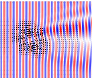
Here, we describe our equations and the processes we model, which we summarise in figure 1.
Set-up for the simulation with parameters  $Ro_{\zeta } = -1.27$,
 $Bu =L_d^2/({\rm \pi} R)^2 = 1.76$, where
 $L_d$ is the Rossby radius of deformation, and
 $K={\rm \pi} R/ \lambda = 3.0$. (a) Normalised vorticity field for an isolated anticyclonic cyclogeostrophic vortex. Black arrows represent the vortex velocity vectors. (b) Height field for a Poincaré wave that is forced from the left side of the domain and interacts with the isolated vortex pictured in (a). The black dash–dotted square in (b) aligns with the bounds of panel (a).

We solve the RSWEs on a square domain of side length  $L_x$, with which we associate a Cartesian coordinate system
 $(x, y)$ centred in the middle of the domain. The layer is under gravitational acceleration
 $g$, has depth
 $H$ at rest and rotates as an
 $f$-plane. These parameters define a non-rotating speed
 $c_0=\sqrt {gH}$ and a Rossby radius of deformation
 $L_d = c_0/f$. The forced–dissipated one-layer RSWEs are
 \begin{equation} \partial_t {\boldsymbol{u}} + \boldsymbol{u} \boldsymbol{\cdot} \boldsymbol{\nabla} \boldsymbol{u} + g\boldsymbol{\nabla} h + f \boldsymbol{\hat{z}} \times \boldsymbol{u} - \mu \nabla^4 \boldsymbol{u} = \boldsymbol{F}_w(x, t) + \boldsymbol{S}_w(x)\end{equation}
and
 \begin{equation} \partial_t h + h \boldsymbol{\nabla} \boldsymbol{\cdot} \boldsymbol{u} + \boldsymbol{u} \boldsymbol{\cdot} \boldsymbol{\nabla} h - \mu \nabla^4h = F_h(x, t) + S_h(x), \end{equation}
where  $\boldsymbol {u} = (u,v)$ is the horizontal velocity field,
 $\boldsymbol {\nabla } = (\partial _{x}, {\partial }_y)$ is the horizontal del operator,
 $\mu$ is the kinematic hyperviscosity (utilised only to provide numerical stability) and
 $h$ is the height of the total water column. The terms
 $\boldsymbol {F}_w$,
 $\boldsymbol {S}_w$,
 $F_h$ and
 $S_h$ on the right-hand sides are wave-forcing and sponge-layer terms, which we describe in more detail later.
Our initial condition consists of an axisymmetric circular vortex centred at the origin of the domain. We achieve this through a three-step process. First, we create a Gaussian vortex in geostrophic balance following
 \begin{equation} \left[u_{\varTheta}^{(0)}, h_{\varTheta}^{(0)}\right] = \left[{\rm \pi}^2fr, \frac{H}{Bu_0}\right]Ro\exp \left(-\frac{r^2}{2(L/{\rm \pi})^2}\right), \end{equation}
where  $u_{\varTheta }^{(0)}$ and
 $h_{\varTheta }^{(0)}$ are the initial tangential velocity and height fields of this vortex,
 $L$ is its characteristic width,
 $Bu_0 = (L_d/L)^2$ is the Burger number and
 $r$ is the distance from the centre of the vortex. While (2.2) is a relatively good approximation for a quasi-geostrophic vortex, water parcels in a vortex with higher
 $Ro$ experience a significant centrifugal acceleration, which modifies the balance. Applying the iterative method of Penven, Halo & Marié (Reference Penven, Halo, Pous and Marié2014), which we detail in Appendix A, to (2.2) yields velocity fields
 $u_{\varTheta }^{(1)}$ and
 $h_{\varTheta }^{(1)}$ that are one step closer to achieving cyclogeostrophic balance. We then use these velocity and height fields as initial conditions for an unforced RSWE simulation. After a transitory adjustment in the form of waves radiating from the vortex and being dissipated by additional sponge layers (see Appendix B), and a rearrangement of the water parcels, a stationary vortex remains. Finally, we save the velocity and height fields
 $u_{\varTheta }^{(2)}$ and
 $h_{\varTheta }^{(2)}$ to be used later as initial conditions for our forced simulations. We repeat this procedure for as many initial vortices as we need. For all simulations,
 $L=25$ km and
 $f=-10^{-4}\ {\rm s}^{-1}$. Note that at the end of this procedure, the vortex has departed from the purely Gaussian shape of (2.2), especially for high Rossby and Burger numbers, for which the adjustment is the strongest.
The adjusted vortex length is defined as  $L_a = {\rm \pi}R$, where
 $R$ is the radius of the maximum tangential velocity
 $U_q=u_{\varTheta }^{(2)}(R)$, as shown in figure 1(a). We define its vorticity Rossby number and bulk Rossby number as
 \begin{equation} Ro_\zeta = \left.\frac{\zeta}{f}\right|_{x=y=0}\quad\text{and}\quad Ro_b = \frac{U_q}{L_af}, \end{equation}
respectively, where  $\zeta = \partial _x v - \partial _y u$ is the vertical vorticity (note that, at this point, no other form of motion is present in the domain).
The resultant azimuthal velocity and vorticity profiles are shown in figure 2. For a given value of  $Ro_b$, cyclogeostrophic balance makes the cyclonic vortices wider than their geostrophic counterparts. For a cyclonic vortex in the southern hemisphere, the inward pressure gradient must balance not only the outward Coriolis force but also the centrifugal force. Thus, a decrease in velocities near the initialised geostrophic value of
 $U_q$ is needed to achieve balance, leading to a wider shape. On the other hand, for anticyclonic vortices, the centrifugal force and pressure gradient are outward and balance the inward Coriolis force. Thus, the velocity increases, leading to a narrower profile (Shakespeare Reference Shakespeare2016).
Azimuthal velocity profiles of a pair of cyclonic (solid blue) and anticyclonic (solid green) vortices that originally started from the same geostrophically balanced velocity profile (solid red) with bulk Rossby number  $Ro_b=0.18$. The final normalised velocity profiles are shown in (a) and the normalised vorticity profiles are shown in (b). The vertical dash–dotted lines correspond to the position
 $x=R$, where the velocity is maximum. The anticyclonic profiles are flipped over the
 $x$-axis to easily compare them with the cyclonic profiles.

In order to capture this cyclonic/anticyclonic asymmetry in the cyclogeostrophic vorticity distributions, which the bulk Rossby number misses, we also measure the enstrophy,  $\varepsilon$, of each vortex, defined below as the integral of the square of the vorticity
 \begin{equation} \varepsilon' = \iint \zeta^2 \,{{\rm d}\kern0.7pt x}\,{{\rm d}y}. \end{equation}
Enstrophy is a convenient method for measuring the strength of the vortex for two reasons. First, the vorticity is the most relevant quantity for scattering. This is expected from ray-tracing theory, which predicts that at leading order in vortex velocity  $U$, the vortical part of the mean flow will rotate the wavevector
 $\boldsymbol {k}$, while the divergent part will only affect the ray paths at a higher order (Bühler Reference Bühler2014, § 4.4.3). This rotation of the wavevector is the main form of scattering that we expect in our experiments. This is consistent with triad resonance theory, which dictates that the dominant triad interaction between the vortex and the wave flow produces a discrete rotation of the wavevector. Second, enstrophy integrates the vorticity over the whole domain and therefore captures some of the information about the spatial structure of the anticyclonic and cyclonic profiles created after cyclogeostrophic adjustment. We non-dimensionalise enstrophy with
 $\varepsilon = \varepsilon ' /(L_a^2f^2)$.
We then generate a plane wave on the boundary at  $x=-L_x/2$, hereafter referred to as the ‘incoming side’. It propagates along
 $x$ with wavenumber
 $\boldsymbol {k}_i = (2{\rm \pi} \lambda ^{-1}, 0)$, where
 $\lambda$ is the wavelength, and frequency
 $\omega _0 = \sqrt {f^2 + c_0^2k_i^2}$ with corresponding period
 $P=2{\rm \pi} \omega _0^{-1}$. We generate this wave via the forcing terms
 \begin{equation} \boldsymbol{F}_w = \tau_w^{{-}1}\left(\boldsymbol{U}_w - \boldsymbol{u}\right)\varPi_w\quad\text{and}\quad F_h = \tau_w^{{-}1}\left(H_w -h \right)\varPi_w, \end{equation}
which first appeared in (2.1a), where  $\tau _w=P$ is the wave restoration time scale. In these forcing terms, the fields
 $(\boldsymbol {u}, h)$ are restored to values
 $(\boldsymbol {U}_w, H_w)$ that satisfy the polarisation relations for Poincaré waves (see Appendix C), that is,
 \begin{equation} \boldsymbol{U}_w = Fr_w c_0 \left(1, \frac{\omega_0}{f}\right)\cos(|\boldsymbol{k}_i| x-\omega_0 t) \quad\text{and}\quad H_w = \frac{|\boldsymbol{k}_i|H}f \sin(|\boldsymbol{k}_i| x-\omega_0 t), \end{equation}
where  $Fr_w = U_w/c_0$ is the wave Froude number, which we keep small throughout this article to keep the waves linear. This forcing occurs over a limited spatial window along
 $x$, following
 \begin{equation} \varPi_w = \varPi(x, -L_x/2 ), \end{equation}
where  $\varPi (x, x_0)$ is a Tukey window that we detail in Appendix B.
At the boundary  $x=+L_x/2$, hereafter referred to as the ‘outgoing side’, a sponge layer absorbs waves through the sponge terms
 \begin{equation} \boldsymbol{S}_w ={-}\tau_s^{{-}1}\boldsymbol{u} \varPi_s\quad\text{and}\quad S_h = \tau_s^{{-}1}(H-h)\varPi_s,\quad\text{where }\varPi_s = \varPi[x, L_x/2-\lambda]\end{equation}
and  $\tau _s=0.05 P$ is the sponge restoration time scale. We verified that the vortex remains unaffected by the wave: for our purposes, it does not move, deform, or lose or gain energy in any detectable manner. The result is a time-independent scattering amplitude pattern induced by the vortex shown in figure 1(b).
2.2. Numerical set-up and experimental design
We use Dedalus (Burns et al. Reference Burns, Vasil, Oishi, Lecoanet and Brown2020) to solve the RSWEs spectrally with periodic boundaries in the horizontal directions. We use  $512$ points in each direction with a uniform spacing of
 ${{\rm d}\kern0.7pt x} = L/50$. The time step is determined by the vortex strength using the Courant–Friedrichs–Lewy condition
 ${\rm d}t < 10^{-2}\, {{\rm d}\kern0.7pt x}/|U_q|$. The simulation time for each experiment is
 $t_{s} = 4t_T/3$, where
 $t_T = L_xk/\omega _0$ is the transit time of the wave phase across the domain. In practice, the phase and group speeds of the incoming waves are similar in magnitude, and thus
 $t_T$ is sufficient time for the wave packets to reach the other side of the domain.
To initialise the simulations, we define the unadjusted ratio of the vortex length scale to the wavelength of the incoming wave  $K_0 = L/\lambda$, which we vary in the range
 $1\leqslant K_0\leqslant 4$. In doing so, we test the consequences of violating the traditional ray-tracing assumption, which requires
 $K_0 \gg 1$. Similarly, we initialise the unadjusted Burger number as
 $Bu_0 = (L_d/L)^2$ from
 $0.5$ to
 $1.5$. McWilliams (Reference McWilliams2016) noted that the size of realistic vortices is around the radius of deformation
 $L_d$. However, we find that they are stable at various scales and explore multiple regimes for completeness. Due to the different adjustment processes between cyclonic and anticyclonic vortices, for a given initial
 $L$, the adjusted length scale ratio
 $K=L_a/\lambda$ is not the same for the cyclonic and anticyclonic simulations. In the end,
 $K$ ranges from
 $0.5$ to
 $4.5$, and similarly the adjusted Burger numbers
 $Bu=(L_d/L_a)^2$ range between
 $0.43$ and
 $2.6$. We use vortices whose values for
 $Ro_\zeta$ vary from
 $-1.27$ to
 $0.89$. We keep
 $Fr_w < 10^{-3}$ for all simulations to avoid nonlinear steepening and wave–wave interactions between the different components of the incoming and scattered waves. Our suite of simulations consists of all combinations of the Rossby numbers, Burger numbers and length scale ratios shown in table 1, resulting in a total of
 $200$ simulations.
Simulation parameters shown as initialisation before adjustments are made.

2.3. Diagnostics
In this section, we show how to extract the scattered wave fields from the simulation outputs. We then demonstrate how to calculate the phase-averaged flux and outline the process for calculating the ratio of wave energy scattered by the vortex.
Because the vortex does not evolve during the course of our simulations, we extract the wave field ( $\boldsymbol {u}_w, h_w$) simply by subtracting the initial conditions from the simulation output, that is,
 $\boldsymbol {u}_w = \boldsymbol {u} - \boldsymbol {u}_{\varTheta }^{(2)}$ and
 $h_w = h - h_{\varTheta }^{(2)}$. After the wave has reached the sponge layer, the sub-domain defined by a square of length
 $4L$ centred at the origin will have a wave field pattern that is constant in time if averaged over one period
 $P$. We define the phase-averaged energy flux density by
 \begin{equation} \boldsymbol{\phi}_X = \frac12c_0^2 \boldsymbol{u_X}\eta_X \quad\text{and}\quad \bar{\boldsymbol{\phi}}_X = \frac1P\left| \int^{t_p + P}_{t_p} \boldsymbol{\phi}_X \,\text{d} t \right|, \end{equation}
where  $\eta _X= h_X - H$ and
 $t_p>0.9t_T$, which ensures that the wave has propagated past the vortex but has not yet wrapped around the periodic boundaries. The subscript
 $X$ indicates which field is used. For example,
 $X=w$ denotes the phase-averaged total wave flux
 $\bar {\boldsymbol {\phi }}_w$, which we show in figure 3(a) for a typical total wave field.
Phase-averaged wave flux for  $(Ro_{\zeta }, Bu, K) = (0.60, 0.44, 4.3)$. The solid blue lines in the control volume are used to calculate the ratio
 $S$ of the scattered wave flux to the incoming wave flux. The vector
 $\boldsymbol {n}_{in}$ (
 $\boldsymbol {n}_{out}$) is the unit vector associated with the incoming (outgoing) boundary. (a) Full wave field
 $\bar {\boldsymbol {\phi }}_w$; (b)
 $y$ component of
 $\bar {\boldsymbol {\phi }}_s$.

To isolate only the flux of the scattered waves  $\bar {\boldsymbol {\phi }}_s$ shown in figure 3(b), we take a two-dimensional Fourier transform of
 $u_w$,
 $v_w$ and
 $h_w$ and cancel the amplitudes of the Fourier modes whose wavevectors are parallel to the incoming wavevector
 $\boldsymbol {k}_i$. We then take an inverse Fourier transform to obtain
 $u_s$,
 $v_s$ and
 $h_s$, which we use to calculate
 $\bar {\boldsymbol {\phi }}_s$ using (2.9a,b).
To calculate the ratio of scattered wave flux to incoming wave flux, we define the control volume shown in figure 3, which is made up of four boundaries located away from the vortex. The incoming boundary is placed at  $x/L = -2$, spans
 $-2\leqslant y/L \leqslant 2$ and has unit normal vector
 $\boldsymbol {n}_{in} = (-1, 0)$. Given that we observe the backscatter to be negligible, all of the energy enters through this boundary. We define the outgoing boundary as a semicircle in the
 $x>0$ half-plane, centred around the origin and of radius
 $x/L = 2$, where virtually all of the energy exits. We denote by
 $\boldsymbol {n}_{out}$ the unit vector normal to this boundary. There is virtually no energy moving through the top and bottom boundaries shown in dashed blue lines.
The total incoming and scattered fluxes are then
 \begin{equation} \varPhi_{in} = \int \bar{\boldsymbol{\phi}}_w \boldsymbol{\cdot} \boldsymbol{n}_{in} \, \text{d}s \quad\text{and}\quad \varPhi_{s} = \int \bar{\boldsymbol{\phi}}_s \boldsymbol{\cdot} \boldsymbol{n}_{out} \,\text{d}s, \end{equation}
integrated along the incoming and outgoing boundaries, respectively. To compare how much energy is scattered between simulations, we define the scattering ratio as
 \begin{equation} S = \varPhi_{s}/\varPhi_{in}. \end{equation}
While this definition excludes the energy in the waves which have scattered back into the incoming direction due to the summation of wavevector rotations, the amount of energy in these waves is likely to be small compared with the total scattered energy. Note that, since the vortex does not evolve in time, triad resonance theory implies that the scattered waves remain at the same frequency as in the incoming wave, and thus wave action and wave energy can be related by a constant (Kafiabad et al. Reference Kafiabad, Savva and Vanneste2019). We will calculate this quantity for all simulations in the next section, and we will use scaling laws to draw a relation from the non-dimensional variables to  $S$.
3. Results
3.1. Scattering pattern
The pattern of the wave flux density magnitude  $|\bar {\boldsymbol {\phi }}_w|$, shown in figure 3(a), consists of an alternating ‘constructive/destructive’ interference pattern in the
 $\{x>0$,
 $y<0\}$ quadrant, with the strongest flux values to be found near the exit of the vortex centre. In the
 $\{x>0$,
 $y>0\}$ quadrant, there is a less well-defined scattering pattern. This qualitatively matches the alternating flux pattern of Dunphy & Lamb (Reference Dunphy and Lamb2014) for a barotropic vortex. We see that there are regions on the outgoing side of the vortex where the flux has dropped to near zero and regions where the flux is more than three times that of the incoming wave.
To explain these features, we show the  $y$-component of the scattered wave flux density,
 $\bar {\boldsymbol {\phi }}_s\boldsymbol {\cdot } \hat {\boldsymbol {y}}$, in figure 3(b). Indeed, isolating the scattered part of the wave field eliminates the distracting interference pattern with the unscattered wave. The
 $y$-component helps us to distinguish three scattered beams. The first one, hereafter referred to as the central scattered beam (CSB), crosses the centre of the vortex. In the cyclonic case presented in figure 3, this beam is characterised by
 $\bar {\boldsymbol {\phi }}_s\boldsymbol {\cdot } \hat {\boldsymbol {y}}<0$. The other two beams emanate from the flanks of the vortex and have
 $\bar {\boldsymbol {\phi }}_s\boldsymbol {\cdot } \hat {\boldsymbol {y}}>0$. We hereafter refer to these beams as right and left scattered beams (RSB and LSB, respectively), in reference to whether they approach the left or right flank of the vortex with respect to the direction of incident wave propagation.
We can now interpret that the region where we see a maximum in  $|\bar {\boldsymbol {\phi }}_s|$ is where constructive interference between the RSB and the CSB takes place. The regions where we find zero flux are created by the RSB and CSB destructively interfering. In experiments with strong vortices, we find lines of destructive interference due to a
 $180^{\circ }$ phase difference between RSB and CSB.
We claim that the scattering direction is mostly controlled by the vorticity. In our simulations, the Coriolis parameter is negative, so the negative vorticity in the centre of the cyclonic vortex produces the CSB, whose dominant wavevector rotates clockwise with respect to the incoming wavevector, and the opposite-sign vorticity region on the outside (recall figure 1a) produces the LSB and RSB, whose wavevector rotates anticlockwise. Similarly, an anticyclonic vortex produces a CSB whose dominant wavevector rotates anticlockwise and produces the LSB and RSB whose wavevectors rotate clockwise. To support this claim, we now compare this pattern with the predictions from ray-tracing equations, which we recall in Appendix D, for an anticyclonic and a cyclonic vortex of similar  $|Ro_\zeta |$ and two different values of
 $K$.
Figure 4 shows that the rays which are initialised to only propagate through the positive/negative vorticity on the vortex edges are rotated anticlockwise/clockwise. The rays which travel through the centre are predominately rotated with the sign of the central vorticity. Thus ray tracing captures the ‘anticlockwise/clockwise/anticlockwise’ scattered beam pattern for cyclonic vortices and the ‘clockwise/anticlockwise/clockwise’ pattern for anticyclonic vortices. There are small differences in the ray-tracing results when we compare cyclonic and anticyclonic vortices that are more than just a flip over the  $y=0$ axis for two reasons. First, anticyclonic vortices are ‘slimmer’ (vorticity is more concentrated near the centre, over a shorter radius) than cyclonic vortices. Second, the refractive effects due to the height field in the term
 ${\rm d}\omega /{\rm d}\kern 0.06em \boldsymbol {x}$ in (D1a,b) differ between cyclonic and anticyclonic vortices. Indeed, an anticyclonic vortex centre rises above the mean depth, and since the group speed
 \begin{equation} c_g = \frac{ghk}{(f^2 + ghk^2)^{1/2}} \end{equation}
increases with depth, the waves travel faster through the centre of the vortex, and thus the height effects make the waves curve away from the centre line  $y=0$. Oppositely, cyclonic vortex centres dip below the mean depth, so height effects make waves curve towards the centre line. We checked that this effect is an order of magnitude smaller than the vorticity effect for balanced vortices.
Full flux field  $\bar {\boldsymbol {\phi }}_w$ for two similar but opposite-signed
 $Ro_\zeta$ and two wavelengths. Here,
 $Bu=0.88$ in all cases. Ray-tracing lines are in black. The green and purple contours correspond to the colour bar shown in figure 1(a). The two dashed blue lines represent the primary scattering angle predicted by triad resonance theory. Panels correspond to parameter values (a)
 $Ro_{\zeta } = 0.60$,
 $K = 3.2$; (b)
 $Ro_{\zeta } = 0.60$,
 $K = 1.07$; (c)
 $Ro_{\zeta } = -0.63$,
 $K = 3.2$; and (d)
 $Ro_{\zeta } = -0.63$,
 $K = 1.07$.

The exact location where the rays converge aligns more closely with constructive interferences between CSB, LSB and RSB, for  $K=3.2$ as opposed to
 $K=1.07$. Note that the ray-tracing predictions do not vary much for the range of
 $K$ explored. Figure 4 reveals that the most striking limitation of ray tracing is that it does not capture the broad angles of scattering, as can be seen from the interference pattern created by the incoming wave and scattered waves.
The triad resonance theory formalism of Ward & Dewar (Reference Ward and Dewar2010) can be used to predict the principal scattering angle  $\theta _p$, that is, the angle made between the incoming wave with wavevector
 $\boldsymbol {k}_i$ and the scattered wave
 $\boldsymbol {k}_s$, which is determined by the main length scale in the vortex
 $\boldsymbol {k_v} = 2{\rm \pi} /L_a$. Assuming
 $|k_i| = |k_s|$, the principal angle can be calculated as a function of
 $K$ as
 \begin{equation} \theta_p = 2 \arcsin((2K)^{{-}1}). \end{equation}
This implies that the angle of scattering would increase for smaller  $K$. For
 $K=1.07$, triad resonance predicts that if there were only one balanced length scale
 $L_a$, the angle of scattering would be
 $65^{\circ }$, which is more than what we measure in our experiments as shown in figure 4. We expect the discrepancy to be due to the multiple length scales and spatial variations of the vorticity field experienced by the part of the plane wave passing through the centre. Thus, even in this simple case, the principal scattering angle is not enough to describe this pattern. Moreover, non-resonant, higher-order interactions would not be captured by triad resonance theory. Thus, neither ray tracing nor triad resonances easily predict the exact nature of the scattering pattern in this simple set-up.
3.2. Scattering statistics
We now summarise the relationship between the scattered ratio  $S$ on the non-dimensional numbers
 $Bu$ and
 $K$, as well as one of the three vortex strength metrics
 $Ro_b$,
 $Ro_{\zeta }$ and
 $\varepsilon$. Visual inspection reveals that for small values of the non-dimensional parameters, the scattering ratio follows power-law relations, while for large values the scattering ratio approaches a maximum of
 $100\,\%$ conversion. The latter is similar to the findings of Dunphy & Lamb (Reference Dunphy and Lamb2014), who carefully checked that their Boussinesq eddies did not exchange net energy with the waves. Therefore, we propose to use an arctan relationship that is linear near the origin and tends to a positive constant towards infinity. We considered several functions, none of which demonstrated superior performance (see Appendix E), and settled on
 \begin{equation} S^{\theta}_Z = \frac{2}{\rm \pi}\arctan(A Z^{\alpha}Bu^{\beta}K^{\gamma}), \end{equation}
where the superscript  $\theta$ denotes the optimised fit,
 $Z \in \{|Ro_b|, |Ro_{\zeta }|, \varepsilon \}$ is a placeholder for the three metrics of vorticity we will test and
 $A$,
 $\alpha$,
 $\beta$ and
 $\gamma$ are the optimisation parameters. To find them, we fit the cyclonic experiments separately from the anticyclonic experiments, and in parallel, for comparison, we fit both datasets together, hereafter referred to as the ‘combined case’. We use the least squares method to find the optimisation parameters using
 $Z = |Ro_b|$, which we show in table 2. We find that all the optimisation parameters have small errors, indicating that our fitting function is appropriate. The combined case is plotted in figure 5, where we have rescaled the data based on the fit parameters. We see that anticyclonic vortices scatter energy at a slightly higher rate, as evidenced by the data points being slightly above the line of perfect fit and as confirmed by table 2. However, the distinction is too small to conclusively claim that this is physical. Thus, we hereafter focus on the combined cases.
Optimisation parameters and their standard deviations for (3.3).

The  $x$-axis shows the data scaled by the fit function and respective optimisation parameters for the (a) enstrophy, (b) bulk Rossby number and (c) vorticity Rossby number. The size of the markers corresponds to the bulk Rossby number, the colours correspond to the adjusted ratio of length scales and the markers correspond to the unadjusted Burger number, as shown in the legend in figure 6. The black dashed lines are perfect fit lines.

We now redo the optimisation using the enstrophy  $\varepsilon$ and the vorticity Rossby number
 $Ro_\zeta$ in addition to the bulk Rossby number
 $Ro_b$. The optimisation parameters for the three vortex strength metrics are shown in table 3. Figure 5 shows the three combined fits scaled by their respective parameters. They appear to be approximately equivalent; however, if we plot the same data on a logarithmic scale (figure 6), we observe that using the vorticity Rossby number
 $Ro_\zeta$ is not as effective as using the enstrophy
 $\varepsilon$ or the bulk Rossby number
 $Ro_b$, which yield closer fits to data points. Both seem to result in round number scaling for
 $\alpha$ as well, with
 $\alpha \approx 2$ if
 $Z = Ro_b$ or
 $\alpha \approx 1$ if
 $Z=\varepsilon$. No matter which measure of vortex strength we use, we find that
 $\beta \approx -1$ and
 $\gamma \approx 2$. Simplifying the dependencies of
 $S$ further, we observe that
 \begin{equation} Ro_b/\sqrt{Bu} = U/\sqrt{gH}=U/c_0 = Fr, \end{equation}
where the last number is the Froude number.
Optimisation parameters using three different vortex strength metrics in place of the bulk Rossby number in (3.3).

The scattering ratio data in figure 5 shown in logarithmic scale. The black dashed lines show perfect fits.

Collecting these approximations, we find that for small values of our non-dimensional parameters, (3.3) simplifies to
 \begin{equation} S\approx 5Fr^2K^2, \end{equation}
which we find to be reasonably accurate up to  $S\approx 0.2$ (see figure 7). This simplified equation breaks down the scattering into a ratio of velocities multiplied by the ratio of length scales.
Simplified scaling for low scattering ratios as a function of only the Froude number  $Fr=Ro_b/\sqrt {Bu}$ and length scale ratio
 $K$.

3.3. Scaling interpretation
Here, we offer a possible interpretation for the seemingly round number scaling for  $Ro$,
 $K$ and
 $Bu$ we found in the previous section. To interpret our results, we turn to Ward & Dewar (Reference Ward and Dewar2010), who derived analytical solutions for a single wave mode interacting with a single-length-scale zero-frequency balanced mode by expressing the RSWEs in the form of interacting triads. In a simplified case, they showed that the amplitude of the scattered wave mode
 $A_s$ increases as a function of the balanced mode amplitude
 $A_v$, the incoming wave mode amplitude
 $A_{in}(t)$ and the interaction coefficient
 $\varGamma$, which is directly derived from the RSWEs. Specifically, this evolution is described by (adapted from Ward & Dewar Reference Ward and Dewar2010, (3.11))
 \begin{equation} \frac{{\rm d}A_s}{{\rm d}t}= 2 \varGamma A_v A_{in}. \end{equation}
Let us start by assuming that the wave mode amplitude is constant in time, which can be achieved to a good approximation if the interaction is weak or brief. Then, we have
 \begin{equation} A_s/A_{in} = 2 \varGamma A_v T_i, \end{equation}
where  $T_i$ is the time scale of the interaction. We can express this equation as a function of our non-dimensional variables. First, the amplitude of the vortex mode is proportional to the bulk Rossby number
 $A_v\propto Ro_b$. Second, while the form of the interaction coefficient is very complicated even for a single triad, Ward & Dewar (Reference Ward and Dewar2010) found that for
 $K \gg \sqrt {Bu}$,
 $\varGamma \propto K$ and for
 $K \ll \sqrt {Bu}$,
 $\varGamma \propto K^2$. In our parameter regime, the Burger numbers are such that
 $0.7 <\sqrt {Bu}=L_d/L< 1.6$, and we use waves with
 $0.5\leqslant K\leqslant 4.5$. We are therefore in an intermediate regime where the scaling
 $\varGamma$ obeys cannot be estimated a priori. As we are about to see, our simulations appear to be closer to a regime where
 $\varGamma \propto K$. Finally, the time scale of this interaction is proportional to the group speed. Note that
 $f$ drops out of the scattering relation, which is because the wave frequencies we examined are high enough compared with
 $|\,f|$, making the waves act more like non-rotating shallow-water waves, and thus all group speeds are close to
 $c_0$. This time scale is then related to the Burger number through
 $T_i \propto 1/c_0 \propto Bu^{-0.5}$. Thus, assuming
 $\varGamma \propto K$, we have
 \begin{equation} S = \varPhi_s/\varPhi_{in}\sim (A_s/A_{in})^2 \propto Ro_b^2 K^2 Bu^{{-}1}, \end{equation}
as we found using our theory-agnostic three-dimensional fits for small values of  $S$.
As the time of interaction increases, the amplitude of the incoming wave decreases and hence the growth rate of the triads progressively decreases. This is an alternative interpretation of the plateau that we see at high values of  $S$, and is why the arctan must be included in our scalings.
Recall that our approximately Gaussian vortex has multiple energetic length scales forming a spectrum of triads, each with their own value of  $\varGamma$. Furthermore, each of the scattered waves that form due to the interaction of the incoming wave can then interact themselves with the vortex to create secondary triads. Thus, the fact that the specific vortex shape that we chose results in very similar scaling to the one-length-scale vortex in Ward & Dewar (Reference Ward and Dewar2010) is remarkable. Furthermore, it may imply that similarly bell-shaped isolated vortices will have similar scalings. In light of these arguments, we expect the details in the way they plateau to be different, but similar isolated vortices likely follow the same growth rates for small values of
 $S$.
4. Discussion and conclusion
We examined the scattering effect induced by an isolated vortex on a plane Poincaré wave. By removing the vortex and the incoming wave, we are able to visualise the scattered wave energy using the wave-averaged flux. The scattered energy forms in an ‘anticlockwise/clockwise/anticlockwise’ (‘clockwise/anticlockwise/clockwise’) pattern, which we attribute to the strong negative (positive) vorticity in the interior for (anti)cyclones and weaker positive (negative) vorticity in the exterior. The ray-tracing equations capture this alternating pattern, but the locations of ray convergence do not always align with the locations of maximum amplitude in the simulation data. We see the expected limitations of ray tracing when the vortex and wavelength are of comparable size, most strikingly when  $K=1$, where the angle of scattering it predicts is much shallower than those we see in the simulations. The scattering pattern of anticyclonic and cyclonic vortices of similar Rossby number magnitude lead to slightly different patterns due to the difference in shape after cyclogeostrophic balance, but the effect is minor in our parameter regime.
Overall, our scattering patterns qualitatively agree with those of the Boussinesq simulations of Dunphy & Lamb (Reference Dunphy and Lamb2014, figure 5) for barotropic vortices, which gives us confidence that RSWEs are a appropriate model for studying IT/vortex interactions. Note that these authors mention that their attempts at interpreting the scattering pattern with ray tracing had failed, leading them to conclude that this approach is not appropriate in their regime. Here, we interpret these ‘hot–cold’ patterns as interference patterns between three scattered beams and the transmitted incident wave, whose general features and directions qualitatively agree with ray-tracing predictions. As such, our interpretation rehabilitates ray tracing to some degree. However, it fails to predict the very existence of a transmitted plane wave, nor can it predict how wide the scattering pattern is, even in experiments with high  $K$ values. Therefore, previous work based on ray tracing (e.g. Rainville & Pinkel Reference Rainville and Pinkel2006; Chavanne et al. Reference Chavanne, Flament, Luther and Gurgel2010) should be interpreted with caution.
On a related subject, figure 8 of the previously cited article shows very different scattering patterns for baroclinic vortices. Interactions between baroclinic modes could yield different results, which could be investigated with multi-layer RSWEs in future studies.
Using three-dimensional fits, we derived a relation that gives the scattering ratio as a function of the Burger number  $Bu$, the ratio of the vortex to the wave length scale
 $K$ and a measure of the vortex strength, which we quantify through the bulk Rossby number
 $Ro_b$, the vorticity Rossby number
 $Ro_\zeta$ and the enstrophy
 $\varepsilon$. We observe that the fit is successful when an
 $\arctan$ is used with a power-law combination of the three non-dimensional numbers as the argument. We find that the bulk Rossby number
 $Ro_b$ and the enstrophy
 $\varepsilon$ are the most suitable vortex strength metrics for predicting the scattering ratio, while the vorticity Rossby number
 $Ro_\zeta$ yields a less suitable approximation. We find round number scalings for the argument in the arctan, specifically,
 $\tan ({\rm \pi} S/2) \propto Ro_b^2K^2Bu^{-1}$. This aligns with the triad formalism from Ward & Dewar (Reference Ward and Dewar2010), where the growth rate of a single triad wave is shown to be proportional to the amplitude of the vortex, which is determined by
 $Ro_b$, the time of interaction, which is determined by
 $Bu$, and the triad interaction coefficient, which is related to
 $K$. Since our theory-agnostic fits using a Gaussian vortex result in the same scaling as the single-mode example in Ward & Dewar (Reference Ward and Dewar2010), it may imply that these scalings would be similar for a variety of isolated vortices with bell-shaped height fields, at least for small values of
 $S$. For small scattering ratios, these dependencies reduce to
 $S\propto Fr^2K^2$.
Independently, Ito & Nakamura (Reference Ito and Nakamura2023) non-dimensionalised the equations of motions first and showed that  $FrK^{-1} = U\lambda /(c_0L)$ can be used to separate the vortical effects on the wave from the linear equations. They varied this parameter as a whole to show different scattering regimes and patterns. At higher values, they showed that the wave can become trapped in the vortex. While their scaling significantly differs from ours, note that we obtained our results by measuring the scattered energy in a theory-agnostic fashion. Furthermore, our scalings are consistent with the theory of Ward & Dewar (Reference Ward and Dewar2010), who found that stronger triads form at large values of
 $K$. Additionally, Coste, Lund & Umeki (Reference Coste, Lund and Umeki1999), who investigated how a vertical vortex in solid-body rotation creates phase dislocations on an incoming wave, found a similar ratio to
 $FrK$.
Although we did not vary  $Fr_w$, we do not anticipate the results to vary until the wave has enough energy to alter the structure of the vortex itself (e.g. via wave capture; see Bühler & McIntyre Reference Bühler and McIntyre2005), or to undergo destabilising nonlinear processes. Study of the nonlinear wave regime is likely to represent an avenue for further research.
Most eddies with characteristic width  $L$ are well approximated by a Gaussian profile within radius
 $L/3$ from their centre (Chelton, Schlax & Samelson Reference Chelton, Schlax and Samelson2011), which makes our scaling relation broadly applicable. To find a more general scaling relation, we could extend our analysis to other vortex profiles and in the process check how robust our scaling relations are to the vortex shape. For example, Flierl (Reference Flierl1988) discusses the stability of axisymmetric vortices whose radial profiles are more general than our Gaussian vortices. We could explore the scattering properties of the stable ones in a future study. We could also use stable oblate vortices (e.g. Young Reference Young1986), which would add another degree of freedom to our scaling relations, and produce asymmetries in the scattering pattern depending on the incoming wave direction.
The parameter range we explored covers a broad range of physical regimes in which an IT will interact with eddies in the ocean. We did not explore waves larger than the vortices, but we can extrapolate from our data that  $K<1$ would lead to little scattering (
 $S<0.1$) even at vorticity Rossby numbers of
 $O(1)$ and Burger numbers of
 $O(0.1)$. We also did not explore simulations with
 $|Ro_\zeta | \gg 1$ and
 $Bu < 0.4$, but since we came close to complete scattering with
 $K=4$, we can extrapolate to find which simulations would lead to completely scattered waves (
 $S=1$). For example, if we had Rossby and Burger numbers equal to one, a wave with
 $K=5$ would already lead to almost complete scattering with
 $S = 0.97$. In open ocean regimes, mesoscale eddies are approximately the size of mode-1 M
 $_2$ tides (
 $K=1$) and have
 $Ro_b = 0.01$ and
 $Bu \approx 1$, so we predict that the scattering will be small at
 $S < 1\,\%$. In submesoscale regimes, near coasts and strong currents, where mode-5 ITs interact with vortices of
 $Ro_b > 0.1$, the scattering ratio will be greater than
 $10\,\%$. These results inspire useful diagnostics for satellite altimetry data and global circulation models to determine where errors may be at their highest given the local vorticity field, IT mode, local rotation rate and stratification. Future work on our idealised model should include simple time-varying balanced flows (e.g. vortex pairs) and oblate vortices and involve adding vertical layers to include the effects of baroclinicity in the balanced flow.
Acknowledgements
We thank J.M. Lilly and three anonymous reviewers for their constructive comments.
Funding
We acknowledge the support of the Natural Sciences and Engineering Research Council of Canada (NSERC), with funding reference numbers RGPIN-2015-03684 and RGPIN-2022-04560.
Declaration of interests
We report no conflict of interest.
Data availability statement
See https://doi.org/10.5281/zenodo.12954100 to find the replication code for this manuscript.
Appendix A. Cyclogeostrophic balance iterative method
To create a time-independent balanced vortex with a non-zero Rossby number we need to include the effects of advection. Thus, the vortex must satisfy
 \begin{equation} \boldsymbol{u} \boldsymbol{\cdot} \boldsymbol{\nabla} \boldsymbol{u} + f \boldsymbol{\hat{z}} \times \boldsymbol{u} ={-}g\boldsymbol{\nabla} \eta. \end{equation}
Equation (A1) can be solved analytically for some axisymmetric cases; however, we can extend this to larger  $Ro$ if we use the iterative method in Penven et al. (Reference Penven, Halo, Pous and Marié2014), which we describe below.
Let the velocity  $\boldsymbol {u_g}$ associated with the geostrophic flow be
 $f \boldsymbol {\hat {z}} \times \boldsymbol {u_g} = -g\boldsymbol {\nabla } \eta$. We rearrange (A1) to give
 \begin{equation} \boldsymbol{u} -\boldsymbol{\hat{z}}\,f^{{-}1} \times (\boldsymbol{u} \boldsymbol{\cdot}\boldsymbol{\nabla} \boldsymbol{u}) = \boldsymbol{u_g}. \end{equation}
It is then possible to approximate the solution by iterating (A2) as follows:
 \begin{equation} \boldsymbol{u}^{(n+1)} = \boldsymbol{u_g} + \boldsymbol{\hat{z}}\,f^{{-}1} \times (\boldsymbol{u}^{(n)} \boldsymbol{\cdot} \boldsymbol{\nabla} \boldsymbol{u}^{(n)}) \end{equation}
while  $\max |\boldsymbol {u}^{(n+1)} - \boldsymbol {u}^{(n)}| < 10^{-4}\ {\rm ms}^{-1}$ or until
 $\boldsymbol {u}^{(n+1)} > \boldsymbol {u}^{(n)}$. These adjusted velocities are used to initialise the velocity field in the vortex simulation.
Appendix B. Sponge layers
The Tukey window is used to force and absorb waves on either side of the domain. It has the profile of a tapered cosine at the edges and a constant at the centre. This is useful to ensure that the waves achieve the amplitude they are prescribed.
The formula for the Tukey window is
 \begin{equation} \varPi(x, x_0) =
\begin{cases} 0, & x < x_0,\\ \dfrac{1}{2}\left\{1 -
\cos\left[\dfrac{2{\rm \pi} x}{\varDelta \lambda}\right]\right\}, &
x_0 \leqslant x < \varDelta \lambda/2 + x_0, \\ 1, & \varDelta
\lambda/2 + x_0 \leqslant x < \lambda - \varDelta \lambda/2+
x_0 , \\ \dfrac{1}{2}\left\{1 - \cos\left[\dfrac{2{\rm \pi}
x}{\varDelta \lambda} - \dfrac{2{\rm \pi}}{\varDelta}\right]
\right\}, & \lambda - \varDelta \lambda/2 + x_0 \leqslant x <
\lambda + x_0 ,\\ 0, & \lambda + x_0 \leqslant x,
\end{cases} \end{equation}
where  $\varDelta = 0.7$.
The vortex adjustment simulation requires a sponge layer to absorb the waves that radiate during the adjustment process. To absorb waves with minimal reflection, a circular sponge layer is set at a distance  $R_1 = 2L$, which increases linearly until
 $R_2=2.8L$ as
 \begin{equation} CS(r) = \begin{cases} 0,
& r\leqslant R_1, \\ (r-R_1)/(R_2-R_1), & R_1 \leqslant r
\leqslant R_2, \\ 1, & R_2 \leqslant r. \end{cases}
\end{equation}
For simulations with high Rossby numbers, there does tend to be some reflection, but it has a small effect on the diagnostics.
Appendix C. Linear shallow-water equations
The linear shallow-water equations are as follows:
 \begin{equation} \partial_t \boldsymbol{u} + f \hat{z} \times \boldsymbol{u} ={-}g \boldsymbol{\nabla} \eta\quad\text{and}\quad \partial_t h + H\boldsymbol{\nabla}\boldsymbol{\cdot} \boldsymbol{u} = 0, \end{equation}
where  $f$ is constant in this article. Let us assume a wave solution that is only propagating in one direction, so that
 $\boldsymbol {V} = [\tilde {u}, \tilde {v}, \tilde {h}]{\rm e}^{{\rm i}kx}$; we can then rewrite (C1a,b) as
 \begin{equation} \partial_t
\boldsymbol{V} + \boldsymbol{\mathsf{M}}\boldsymbol{V} =
0,\quad\text{where}\ \boldsymbol{\mathsf{M}} = \begin{bmatrix} 0 &
-f & {\rm i}kg\\ f & 0 & 0 \\ {\rm i}kH & 0 & 0
\end{bmatrix}.
\end{equation}
The three eigenvalues of  $M$ are proportional to the frequencies of the wave modes. They are
 $\omega _G = 0$ and
 $\omega ^{(\pm )}_{W} = \pm \sqrt {f^2 + gHk^2}$, with corresponding eigenvectors
 \begin{equation} \boldsymbol{G} = \left[0, 1, -\dfrac{{\rm i}f}{gk}\right] \quad\text{and} \quad \boldsymbol{W}_{{\pm}} = \left[\dfrac{\omega^{({\pm})}_W}{f}, 1, \dfrac{-{\rm i}kH}{f}\right]. \end{equation}
The eigenvectors  $\boldsymbol{W}_{\pm }$ are used to force the wave from the right.
Appendix D. Ray tracing
Ray tracing is a method to track the position and wavevector of a wave packet through a fluid medium, assuming that the wavelength is small compared with the length scales in the medium. Let the position of the wave packet be  $\boldsymbol {x}$ with wavevector
 $\boldsymbol {k}$, and let it be made to pass through a velocity field
 $\boldsymbol {U} = (U, V)$; then the ray-tracing equations read
 \begin{equation} {\rm d}\kern 0.06em \boldsymbol{x}/{\rm d}t = U + {\rm d}\omega/{\rm d}\boldsymbol{k}\quad\text{and}\quad {\rm d}\boldsymbol{k}/{\rm d}t ={-}(\boldsymbol{\nabla}\boldsymbol{U}) \boldsymbol{\cdot} \boldsymbol{k} - {\rm d}\omega/{\rm d}\kern 0.06em \boldsymbol{x}, \end{equation}
where  $\omega = \sqrt {f^2 + gh\boldsymbol {k}^2}$. The first equation describes the evolution of the wave packet position due to the advection of the media and the group speed. The second equation describes the refraction of the wavevector as a result of strain and shear and due to the change in frequency.
Appendix E. Alternative fitting functions
Here, we explore two other choices for fitting function which are linear for small values of  $S$ and then plateau towards one, namely a sigmoid and a tanh defined as
 $$\begin{gather} \breve{S}^{\theta}_Z= 2(1 + \exp[{-}A Z^{\alpha}Bu^{\beta}K^{\gamma}]), \end{gather}$$
 $$\begin{gather}\check{S}^{\theta}_Z= \tanh [A Z^{\alpha}Bu^{\beta}K^{\gamma}]. \end{gather}$$
The curves for these functions are shown in figure 8(a) and the fit parameters are shown in table 4. We find that the fit parameters for both the sigmoid and the tanh can no longer be rounded to whole numbers as we were able to do using arctan. Furthermore, the fit has become worse for both these functions, as shown in figure 8(b) for the sigmoid (to compare with figure 6), because both functions plateau too quickly, resulting in inaccurate fitting for low values of  $S$. While the arctan we use in the main text models the data well for all values of
 $S$, we do not believe this implies that there is something physical about arctan, but rather that it is likely just a convenient choice to model the plateau.
(a) Fitting curves. (b) Sigmoid fit using the same legend as in figure 6.

Optimisation parameters for alternative fitting functions using  $Z=Ro_b$.



 Open access

