

1 Introduction
Separated flows over lifting surfaces have been studied extensively due to their critical importance in aerodynamics and hydrodynamics. Substantial researches have been dedicated to the understanding of separated flows over canonical airfoils to reveal the separation mechanism and their influences on the aerodynamic characteristics (Anderson Reference Anderson2010). In many of the fundamental studies, the assumption of two-dimensional (or quasi-two-dimensional) flow was applied to assess the performance of airfoils, offering valuable insights (Abbott & Von Doenhoff Reference Abbott and Von Doenhoff1959; Pauley, Moin & Reynolds Reference Pauley, Moin and Reynolds1990; Huang et al. Reference Huang, Wu, Jeng and Chen2001; Yarusevych, Sullivan & Kawall Reference Yarusevych, Sullivan and Kawall2009; He et al. Reference He, Gioria, Pérez and Theofilis2017a; Rossi et al. Reference Rossi, Colagrossi, Oger and Le Touzé2018).
Over the past couple of decades, there have been a large number of studies focusing on three-dimensional post-stall flows at angles of attack much higher than those traditionally considered. These studies were performed to examine fundamental aspects of flows related to biological fliers and swimmers as well as small-scale aircraft that experience large-amplitude perturbations in flight (Ellington et al. Reference Ellington, Van Den Berg, Willmott and Thomas1996; Dickinson, Lehmann & Sane Reference Dickinson, Lehmann and Sane1999; Eldredge & Jones Reference Eldredge and Jones2019). The lifting surfaces for these flows have some unique properties. The wings have low-aspect-ratio planforms and generate prominent tip vortices at high angles of attack (Lentink & Dickinson Reference Lentink and Dickinson2009; Taira & Colonius Reference Taira and Colonius2009). For these reasons, the resulting wakes are highly three-dimensional with complex nonlinear dynamics generated by the interactions among the wake vortices. Under the tip effects, the wake dynamics of finite wings can be significantly different from its two-dimensional analogue. The three-dimensional nature of the wakes requires global analysis of the separation dynamics.
Separated flows over finite-aspect-ratio wings in pure translation have been examined with surface oil visualizations (Gregory et al. Reference Gregory, Quincey, OReilly and Hall1971; Wang Reference Wang1976; Winkelmann et al. Reference Winkelmann, Barlow, Saini, Anderson and Jones1980). From these visualizations, Winkelmann & Barlow (Reference Winkelmann and Barlow1980) proposed a flow field model for a post-stall rectangular wing. This model consists of a pair of counter-rotating tip vortices at the two ends of the wing and the mushroom-like three-dimensional separation bubble. Later, by smoke visualization, Freymuth, Bank & Finaish (Reference Freymuth, Bank and Finaish1987) revealed the intricate three-dimensional wake structures behind finite wings. On the aerodynamic characterizations of low-aspect-ratio wings at low Reynolds numbers, Pelletier & Mueller (Reference Pelletier and Mueller2000), Torres & Mueller (Reference Torres and Mueller2004) and Ananda, Sukumar & Selig (Reference Ananda, Sukumar and Selig2015) obtained a wealth of force and pitching moment data for a large collection of aspect ratios, angles of attack and planform geometries.
Direct numerical simulations have provided detailed insights into separated flows over finite-aspect-ratio wings in translation. The wake structures behind an impulsively started plate were analysed by Taira & Colonius (Reference Taira and Colonius2009) using direct numerical simulation at Reynolds numbers of 300 and 500. In the initial stage of wake development, the wake vortices share the same structures for all aspect ratios. At large time, the tip vortices significantly influence the vortex dynamics and the corresponding forces on the wings. The long-term stability of the wake was found to be dependent on the angle of attack, aspect ratio and the Reynolds number. Lee et al. (Reference Lee, Hsieh, Chang and Chu2012) applied the force element theory (Chang Reference Chang1992) to the impulsively started flows around low-aspect-ratio wings and identified the wake regions responsible for the force generation. They have shown that the tip vortices exert lift force during the start-up manoeuvre. Tong, Yang & Wang (Reference Tong, Yang and Wang2020) characterized the three-dimensional flow over a flat-plate using the vortex-surface fields. This Lagrangian-based structure identification method revealed how the leading-edge vortex evolve into hairpin-like structures in the wake. For higher Reynolds number flows, Garmann & Visbal (Reference Garmann and Visbal2017) conducted high-fidelity large eddy simulations of flow over finite-aspect-ratio wings at  $Re=2\times 10^{5}$. Intricate details of the vortical structures near the wing tip were revealed.
More recently, stability analysis has been carried out to study the instabilities in the wake of finite-aspect-ratio wings. He et al. (Reference He, Tendero, Paredes and Theofilis2017b) conducted linear stability analysis on the flows over finite elliptical wings. Two classes of linearly unstable perturbations were identified, namely the highly amplified symmetric modes and the weakly amplified antisymmetric disturbances. Navrose, Brion & Jacquin (Reference Brion and Jacquin2019) performed transient growth analysis on the wake of finite NACA 0012 wings. The optimal linear perturbation was found to be located near the surface of the wing in the form of chordwise periodic structures whose strength decreases from the root towards the tip.
As one of the key features in a finite wing wake, the tip vortex by itself has also gained considerable attention (Spalart Reference Spalart1998). The lifting line theory models the tip vortices as a pair of counter-rotating vortex lines linked to the starting vortex in the far wake, and connected by the ‘bound’ vortex on the wing, thus forming a closed loop (Anderson Reference Anderson1999). Over the years, more detailed investigations have been carried out to reveal the formation, evolution and instability mechanisms of the tip vortices (McCormick, Sherrier & Tangler Reference McCormick, Sherrier and Tangler1968; Crow Reference Crow1970; Francis & Kennedy Reference Francis and Kennedy1979; Katz & Galdo Reference Katz and Galdo1989; Green & Acosta Reference Green and Acosta1991; Devenport et al. Reference Devenport, Rife, Liapis and Follin1996; Birch et al. Reference Birch, Lee, Mokhtarian and Kafyeke2004; Duraisamy Reference Duraisamy2005; Giuni Reference Giuni2013; Edstrand et al. Reference Edstrand, Davis, Schmid, Taira and Cattafesta2016, Reference Edstrand, Schmid, Taira and Cattafesta2018a). Based on the insights from these studies, various control techniques to alleviate the tip vortices have also been developed to reduce the induced drag and wake vortex hazards (Gursul et al. Reference Gursul, Vardaki, Margaris and Wang2007; Greenblatt Reference Greenblatt2012; Edstrand et al. Reference Edstrand, Sun, Schmid, Taira and Cattafesta2018b; Gursul & Wang Reference Gursul and Wang2018).
We note that the three-dimensional separated flows over finite-aspect-ratio wings have also been extensively studied for wings under unsteady manoeuvres, including surging (Chen, Colonius & Taira Reference Chen, Colonius and Taira2010; Mancini et al. Reference Mancini, Manar, Granlund, Ol and Jones2015), rotation/revolving (Lentink & Dickinson Reference Lentink and Dickinson2009; Harbig, Sheridan & Thompson Reference Harbig, Sheridan and Thompson2013; Garmann & Visbal Reference Garmann and Visbal2014; Jones et al. Reference Jones, Medina, Spooner and Mulleners2016; Jardin Reference Jardin2017), pitching (Buchholz & Smits Reference Buchholz and Smits2006; Green & Smits Reference Green and Smits2008; Yilmaz & Rockwell Reference Yilmaz and Rockwell2012; Jantzen et al. Reference Jantzen, Taira, Granlund and Ol2014), heaving/plunging (Visbal, Yilmaz & Rockwell Reference Visbal, Yilmaz and Rockwell2013; Akkala & Buchholz Reference Akkala and Buchholz2017) and flapping motions (Birch & Dickinson Reference Birch and Dickinson2001; Dong, Mittal & Najjar Reference Dong, Mittal and Najjar2006; Shyy et al. Reference Shyy, Aono, Chimakurthi, Trizila, Kang, Cesnik and Liu2010). These studies have closely examined the formation of large-scale vortical structures, with particular emphasis on the leading-edge vortex (LEV) and its influence on added lift (Eldredge & Jones Reference Eldredge and Jones2019). These unsteady motions generate significantly larger lift than that in the steadily translating wings. However, such lift enhancement is short-lived, except for rotating wings with low aspect ratio, for which the high lift is sustained by the attached LEV (Manar et al. Reference Manar, Mancini, Mayo and Jones2015; Percin & Van Oudheusden Reference Percin and Van Oudheusden2015).
Despite the vast literature, there are still fundamental questions left unanswered concerning three-dimensional separated flows over finite-aspect-ratio wings in pure translation. It is generally known that the three-dimensional wake dynamics described in the previous works are closely related with the tip effects. However, the detailed process of how the tip-imposed three dimensionality is introduced into the flow remains elusive. The formation of the wake vortical structures under the tip effects, as well as the dynamical relations between those structures requires further analysis.
To address the aforementioned questions, we carry out a large number of direct numerical simulations of flows over finite-aspect-ratio NACA 0015 wings. By focusing on the development of the three-dimensional wake, we characterize the tip effects on separation and wake dynamics. In what follows, we present the computational set-up and its validation in § 2. The results are discussed in § 3 starting with the flow physics on the wing surface in § 3.1. A detailed look at the three-dimensional wake structures is provided in § 3.2, followed by the spectral analysis of the wake in § 3.3. A classification of the wake states for cases with different angles of attack and aspect ratios is provided § 3.4. The aerodynamic forces and their relationship with the wake dynamics are presented in § 3.5. We conclude this study by summarizing our findings in § 4.
2 Computational set-up
2.1 Numerical approach
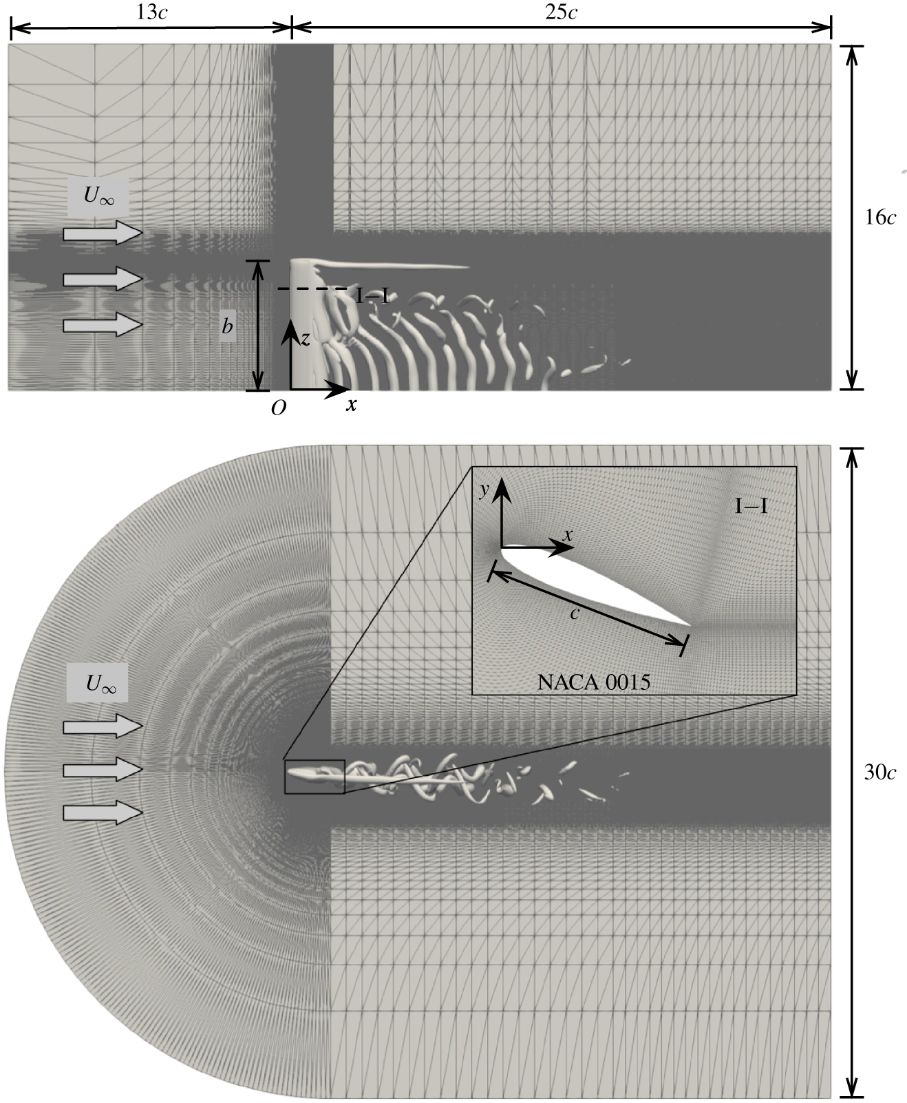
We numerically analyse incompressible flow over a NACA 0015 wing with a straight cut tip. The wing is situated in uniform flow with velocity  $U_{\infty }$ as shown in figure 1. The three-dimensional flow over the finite wing is studied by numerically solving the Navier–Stokes equations
 $$\begin{eqnarray}\displaystyle & \displaystyle \frac{\unicode[STIX]{x2202}\boldsymbol{u}}{\unicode[STIX]{x2202}t}+\boldsymbol{u}\boldsymbol{\cdot }\unicode[STIX]{x1D735}\boldsymbol{u}=-\unicode[STIX]{x1D735}p+\frac{1}{Re}\unicode[STIX]{x1D6FB}^{2}\boldsymbol{u}, & \displaystyle\end{eqnarray}$$
 $$\begin{eqnarray}\displaystyle & \displaystyle \unicode[STIX]{x1D735}\boldsymbol{\cdot }\boldsymbol{u}=0, & \displaystyle\end{eqnarray}$$
 $\boldsymbol{u}=(u_{x},u_{y},u_{z})$ is the velocity vector and
 $p$ is the pressure. An incompressible flow solver Cliff (in CharLES software package, Cascade Technologies, Inc.) is used in the present study. This solver employs a collocated, node-based finite volume method to compute the solutions to the governing mass and momentum equations. A fractional step scheme is used for the time integration. To enforce mass conservation, a corrector step is performed after solving the momentum equations to solve the pressure Poisson equation, thus providing a solenoidal velocity field which also satisfies the momentum equations. Further details of the solver can be found in Ham & Iaccarino (Reference Ham and Iaccarino2004) and Ham, Mattsson & Iaccarino (Reference Ham, Mattsson and Iaccarino2006).
The computational set-up for the case of  $(\unicode[STIX]{x1D6FC},sAR)=(22^{\circ },6)$.

For non-dimensionalization, we normalize the spatial variables by the chord length  $c$, the velocities by the free stream velocity
 $U_{\infty }$ and the time by
 $c/U_{\infty }$. The Reynolds number in the momentum equation (2.1) is defined as
 $Re\equiv U_{\infty }c/\unicode[STIX]{x1D708}$, where
 $\unicode[STIX]{x1D708}$ is the kinematic viscosity. In this work, we set the Reynolds number to
 $Re=400$, which is sufficiently low for the flow to remain laminar but high enough to trigger the wake unsteadiness. As we are interested in the three-dimensional flow physics imposed by the tip effects, we simulate the half-wing model by prescribing the symmetry boundary condition along the midspan. Denoting half-span as
 $b$, the semi aspect ratio is defined as
 $sAR=b/c$ and is varied from 1 to 6, which allows us to study the spanwise variation of the separated flows under tip effects. The angle of attack
 $\unicode[STIX]{x1D6FC}$ is varied from
 $0^{\circ }$ to
 $30^{\circ }$.
The computational domain covers  $(x,y,z)\in [-13,25]\times [-15,15]\times [0,16]$, where
 $x$,
 $y$ and
 $z$ are the streamwise, cross-flow and spanwise coordinates. This results in a maximum blockage ratio of 0.8 % for the case of
 $(\unicode[STIX]{x1D6FC},sAR)=(30^{\circ },6)$. We note that doubling the domain size in all three directions yields no noticeable difference in the time histories of the lift and drag forces. The origin of the Cartesian coordinate system is placed at the leading edge of the wing on the midspan plane (
 $z=0$) plane. The computational domain is discretized with a C-type grid with the mesh refined in the vicinity of the wing as well as its wake. The adequacy of the grid resolution is examined in § 2.2.
The inlet and far-field boundaries are prescribed with free stream  $\boldsymbol{u}=(U_{\infty },0,0)$. The convective boundary condition (
 $\unicode[STIX]{x2202}\boldsymbol{u}/\unicode[STIX]{x2202}t+U_{\infty }\unicode[STIX]{x2202}\boldsymbol{u}/\unicode[STIX]{x2202}x=0$) is applied at the outlet to allow wake structures to leave the domain without disturbing the near-field flow. The wing surface is treated with the no-slip boundary condition. The simulations are started with uniform flow, and statistics are recorded only after the initial transients are flushed out of the computational domain (typically 25 convective time units). Flow statistics are collected with over 100 convective time units to ensure statistical convergence.
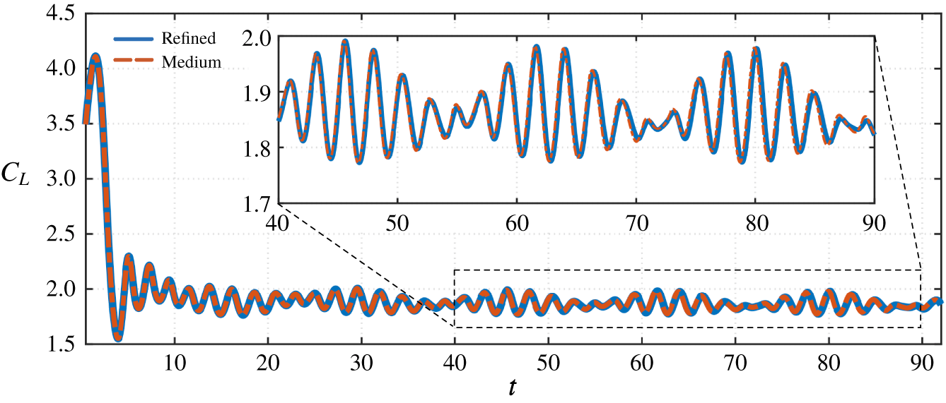
Time histories of the lift coefficient obtained from two sets of meshes for the case of  $(\unicode[STIX]{x1D6FC},sAR)=(22^{\circ },6)$.

Set-ups for the different meshes for the case of  $(\unicode[STIX]{x1D6FC},sAR)=(22^{\circ },6)$. Here,
 $N_{p}$ and
 $N_{s}$ are the numbers of grid points on the pressure and suction side of the airfoil. The number of grids along the wing span is
 $N_{z}$. The total number of control volumes is
 $N_{CV}$ and CFL is the Courant number used in the simulations.

2.2 Verification and validation
To verify the convergence of the numerical results with respect to the grid resolution, we examine the case of  $(\unicode[STIX]{x1D6FC},sAR)=(22^{\circ },6)$ with two sets of meshes listed in table 1. For the refined mesh, the temporal resolution is also increased by restricting the maximum CFL number to be half of the medium mesh. We compare the forces on the wing evaluated from the two meshes to assess the mesh requirement. The time history of the lift force obtained from these meshes are reported in figure 2. Throughout this study, the lift and drag forces are reported in their non-dimensional forms through
 $$\begin{eqnarray}C_{L}=\frac{\displaystyle \int _{S}(-p\boldsymbol{n}+\unicode[STIX]{x1D749})\boldsymbol{\cdot }\boldsymbol{e}_{\boldsymbol{y}}\,\text{d}S}{{\textstyle \frac{1}{2}}U_{\infty }^{2}bc}\quad \text{and}\quad C_{D}=\frac{\displaystyle \int _{S}(-p\boldsymbol{n}+\unicode[STIX]{x1D749})\boldsymbol{\cdot }\boldsymbol{e}_{\boldsymbol{x}}\,\text{d}S}{{\textstyle \frac{1}{2}}U_{\infty }^{2}bc},\end{eqnarray}$$
where  $S$ denotes the wing surface,
 $\boldsymbol{n}$ is the unit normal vector pointing outward from the wing surface. Unit vectors
 $\boldsymbol{e}_{\boldsymbol{y}}$ and
 $\boldsymbol{e}_{\boldsymbol{x}}$ are in the lift and drag directions, respectively. Moreover,
 $\unicode[STIX]{x1D749}=\unicode[STIX]{x1D707}\unicode[STIX]{x1D74E}\times \boldsymbol{n}$ is the skin-friction vector (
 $\unicode[STIX]{x1D707}$ is the dynamic viscosity of fluid and
 $\unicode[STIX]{x1D74E}=\unicode[STIX]{x1D735}\times \boldsymbol{u}$ is the vorticity vector). Once the initial transient dynamics settles (from the use of uniform flow as the initial condition), the lift coefficients exhibit quasi-periodic oscillations with low-frequency beating. This is resolved well with both mesh resolutions even at large times. Thus, the medium resolution grid is deemed adequate to yield accurate results and is used throughout this study.
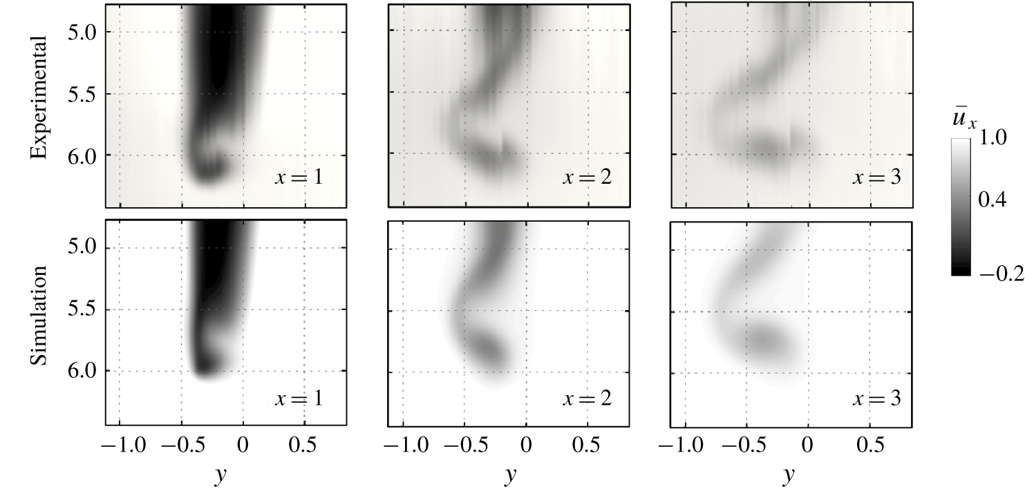
To validate our computational set-up, we compare the numerical results against the stereoscopic particle image velocimetry (known as SPIV) measurements from water tunnel experiments conducted at the Rensselaer Institute. Detailed descriptions of the experimental set-up are documented in Hayostek & Amitay (Reference Hayostek and Amitay2018). In contrast to the symmetry boundary condition used for the midspan in the present simulations, a wall is present at the root plane in the water tunnel. For this reason, comparison between the numerical and experimental results is focused near the tip region for the case of  $(\unicode[STIX]{x1D6FC},sAR)=(22^{\circ },6)$, where the influence of the root boundary condition is small. The time-averaged streamwise velocity fields are shown in figure 3 for three streamwise locations at
 $x=1$, 2 and 3. While the water tunnel experiments are conducted at a larger Reynolds number of 600, the flow remains laminar and is in good agreement with that from the present numerical simulation, confirming the fidelity of the numerical results.
Comparison of time-averaged streamwise velocity  $\overline{u}_{x}$ between the experiment and the present simulation at selected streamwise locations aft of a wing of
 $(\unicode[STIX]{x1D6FC},Re)=(22^{\circ },6)$. The experiments are conducted at
 $Re=600$ in the water tunnel at the Rensselaer Polytechnic Institute, while the numerical simulation is performed at
 $Re=400$.

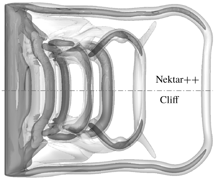
We further validate the present numerical results against those from another flow solver Nektar++ that is based on the spectral/hp element method (Cantwell et al. Reference Cantwell, Moxey, Comerford, Bolis, Rocco, Mengaldo, De Grazia, Yakovlev, Lombard and Ekelschot2015). The computation is carried out with an independent numerical set-up (He et al. Reference He, Burtsev, Theofilis, Zhang, Taira, Hayostek and Amitay2019; Zhang et al. Reference Zhang, Taira, Hayostek, Amitay, He and Theofilis2019). We compare the wake vortical structures obtained by Nektar++ (top) and Cliff (bottom) for the same case of  $(\unicode[STIX]{x1D6FC},sAR)=(22^{\circ },4)$ at
 $t=9.25$ in figure 4. Shown are the isosurfaces of
 $\Vert \unicode[STIX]{x1D74E}\Vert =1$ (vorticity magnitude) and
 $Q=1$ (second invariant of velocity gradient tensor). The vortical structures obtained from the two solvers agree in an excellent manner with each other even for the smallest flow details. Based on the above verification and validation, we have ensured that the current computational set-up is reliable. We now proceed to present our results below.
Comparison of the vortical structures obtained from Nektar++ (top) and Cliff (bottom) at  $t=9.25$ for the case
 $(\unicode[STIX]{x1D6FC},sAR)=(22^{\circ },4)$. Both simulations are started with uniform initial condition. Shown are isosurfaces of
 $\Vert \unicode[STIX]{x1D74E}\Vert =1$ in transparent grey and
 $Q=1$ in dark grey.

Perspective view the vortical structures for the case of  $(\unicode[STIX]{x1D6FC},sAR)=(22^{\circ },4)$. Isosurfaces of
 $Q=1$ are shown in dark grey to visualize vortex cores and
 $\Vert \unicode[STIX]{x1D714}\Vert =2$ in transparent grey to represent the vorticity sheet.

3 Results
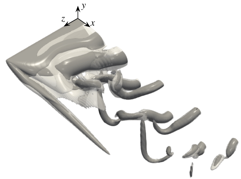
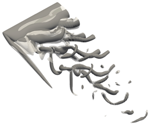
The wake behind a finite-aspect-ratio wing exhibits rich three-dimensional flow features due to the tip effects, as shown in figure 5. In this section, we begin the discussions by focusing on the wing surface to look for the source of vorticity. Next, we describe in detail the three-dimensional wake dynamics. The aerodynamic forces are also discussed with an emphasis on their relationship with the three-dimensional wake structures.
3.1 Boundary vorticity flux and skin-friction lines
We begin our analysis by examining the introduction of vorticity to the flow from the wing surface. In incompressible flow, vorticity is only generated on the solid surface and diffuses into the flow (Morton Reference Morton1984; Hornung Reference Hornung1989; Wu, Ma & Zhou Reference Wu, Ma and Zhou2007). The rate at which vorticity is created at the surface is given by the wall-normal boundary vorticity flux
 $$\begin{eqnarray}\unicode[STIX]{x1D748}=-\unicode[STIX]{x1D708}\boldsymbol{n}\boldsymbol{\cdot }\unicode[STIX]{x1D72E},\end{eqnarray}$$
where  $\unicode[STIX]{x1D72E}=(\unicode[STIX]{x1D735}\unicode[STIX]{x1D74E})_{0}$ is the vorticity gradient tensor at the surface.
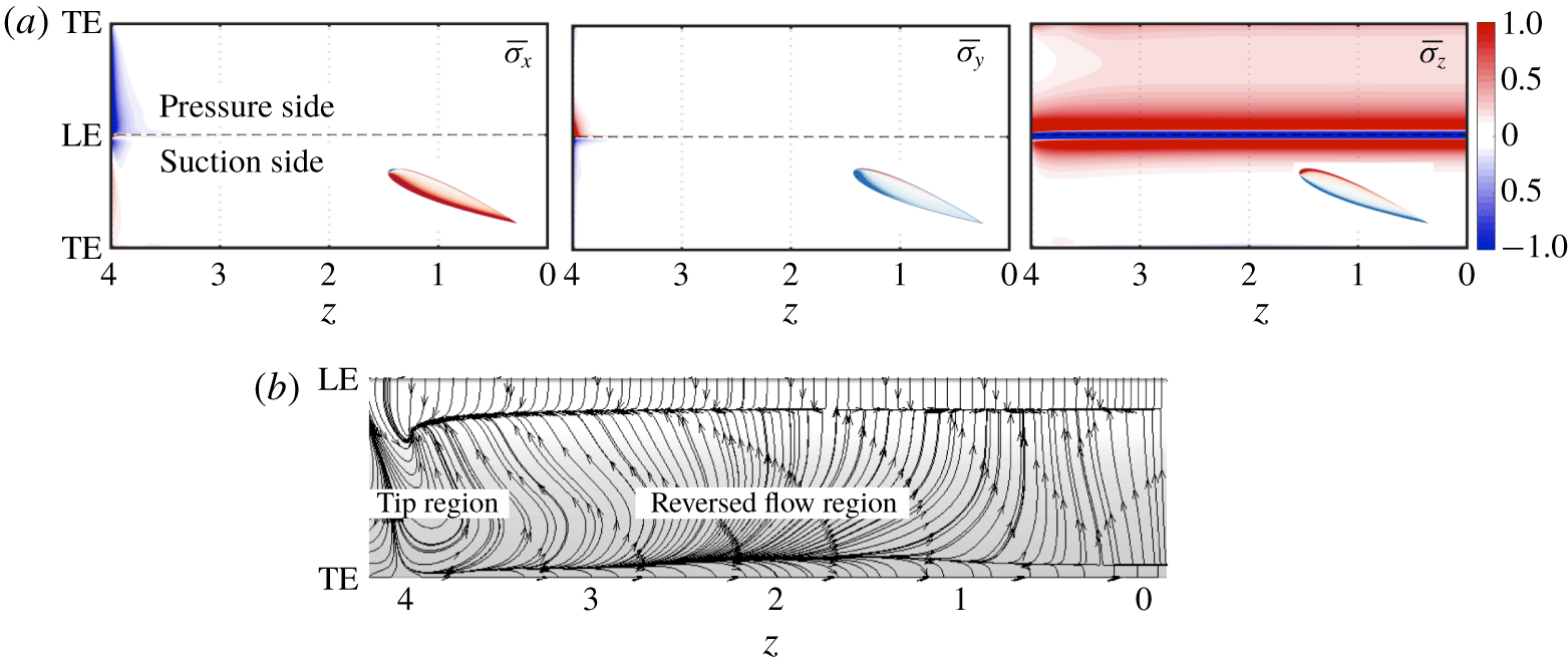
Time-averaged flow behaviour at the wing surface for  $(\unicode[STIX]{x1D6FC},sAR)=(22^{\circ },4)$. (a) Three components of the wall-normal boundary vorticity flux. The surface of the wing is unfolded to a plane by cutting along the trailing edge, TE. The dashed line indicates the leading edge, LE, of the wing. The insets show the boundary vorticity flux on the side surface. (b) Skin-friction lines on the suction surface.

Let us show the vorticity flux along the wing surface for a representative case of  $(\unicode[STIX]{x1D6FC},sAR)=(22^{\circ },4)$. The time-averaged wall-normal boundary vorticity flux components
 $\overline{\unicode[STIX]{x1D70E}}_{x}$,
 $\overline{\unicode[STIX]{x1D70E}}_{y}$ and
 $\overline{\unicode[STIX]{x1D70E}}_{z}$ are plotted in figure 6(a) to identify the local generation of vorticity. As expected, the spanwise vorticity flux
 $\overline{\unicode[STIX]{x1D70E}}_{z}$ dominates over the surface of the wing. Negative
 $\overline{\unicode[STIX]{x1D70E}}_{z}$ is contained within a narrow region along the leading edge of the wing. This region injects a large amount of negative
 $\unicode[STIX]{x1D714}_{z}$ into the flow, forming the leading-edge vortex sheet. Compared to
 $\overline{\unicode[STIX]{x1D70E}}_{z}$, the other two components of the vorticity flux appear negligible for the majority of the span. It is only at the close vicinity of the wing tip that considerable level of
 $\overline{\unicode[STIX]{x1D70E}}_{x}$ and
 $\overline{\unicode[STIX]{x1D70E}}_{y}$ can be found. The creation of vorticity on the finite-aspect-ratio wing is not strongly affected by the tip effects and is predominantly two-dimensional along the span. There is also vorticity generation on the side surface of the wing tip. However, vorticity generated from the side does not appear to play a major role. Similar tip vortical structures are also found in simulated flows over finite flat-plates of zero thickness (Taira & Colonius Reference Taira and Colonius2009).
Once the vorticity is generated at the wing surface, it is diffused into the flow and is convected by the free stream. The developed flow imprints the skin-friction field  $\unicode[STIX]{x1D749}$ on the wall, as shown in figure 6(b). Three regions can be recognized from the skin-friction field. The region close to the leading edge away from the tip is occupied by the nearly two-dimensional boundary layer, which separates from the wing in a uniform manner. Post separation, a region of reversed flow appears on the suction side of the wing where the skin-friction lines exhibit spanwise component of the flow. The dominant three dimensionality is observed over the wing tip region with a three-dimensional swirl pattern, as reported in the experimental work of Winkelmann & Barlow (Reference Winkelmann and Barlow1980).
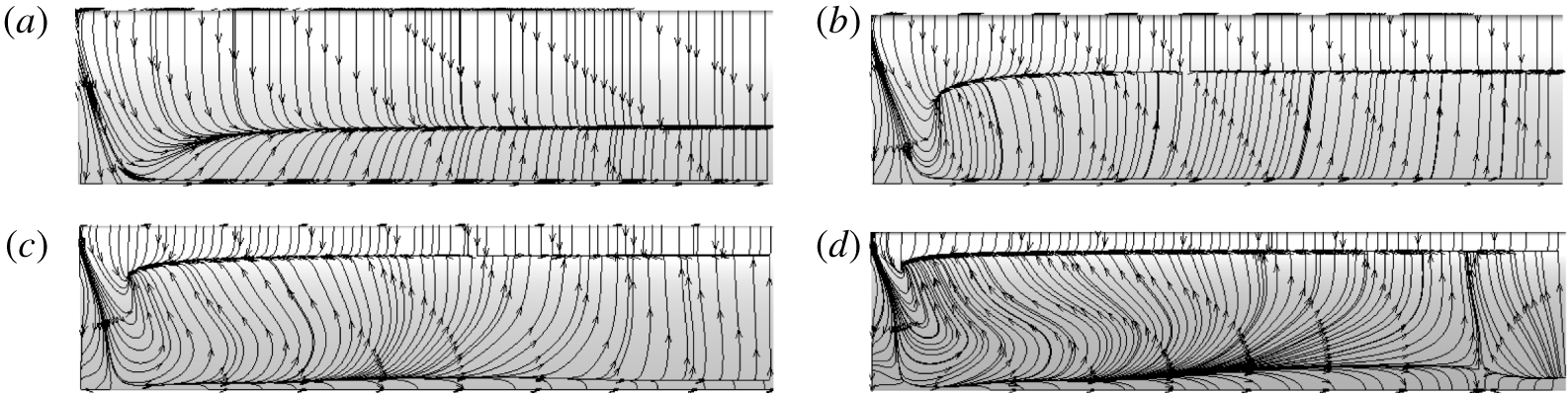
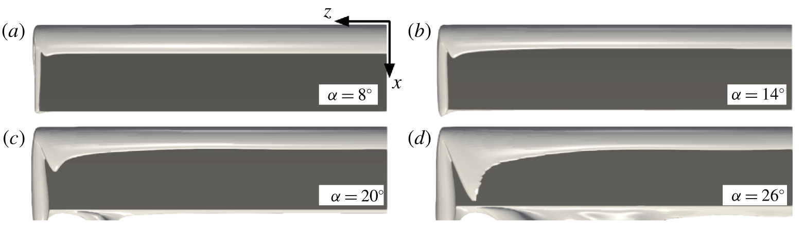
Time-averaged skin-friction line patterns on the suction side for the cases of  $sAR=4$ for (a)
 $\unicode[STIX]{x1D6FC}=8^{\circ }$, (b)
 $\unicode[STIX]{x1D6FC}=14^{\circ }$, (c)
 $\unicode[STIX]{x1D6FC}=20^{\circ }$ and (d)
 $\unicode[STIX]{x1D6FC}=26^{\circ }$.

To assess the influence of the angle of attack on the near-surface flow pattern, we visualize the time-averaged skin-friction lines for the cases of  $sAR=4$ with different
 $\unicode[STIX]{x1D6FC}$ in figure 7. For higher angles of attack, the flow separation occurs more upstream, and the spanwise extent of the boundary layer that is affected by the tip effects becomes smaller. The skin-friction lines in the recirculation region becomes more three-dimensional at higher
 $\unicode[STIX]{x1D6FC}$.
The development of the three-dimensional flow can be envisioned from the boundary vorticity flux and skin-friction lines. Vorticity is introduced from the wing surface in a predominantly two-dimensional manner. The vortex sheets emanate from the leading edge and the wing tip. While the roll-up of the leading-edge vortex sheet is two-dimensional, the roll-up from the tip is fundamentally three-dimensional yielding a streamwise tip vortex. As the tip vortex develops, its influence grows from being locally confined to imposing spanwise variations, as evident in figure 5. We discuss the three-dimensional wake dynamics in the following sections.
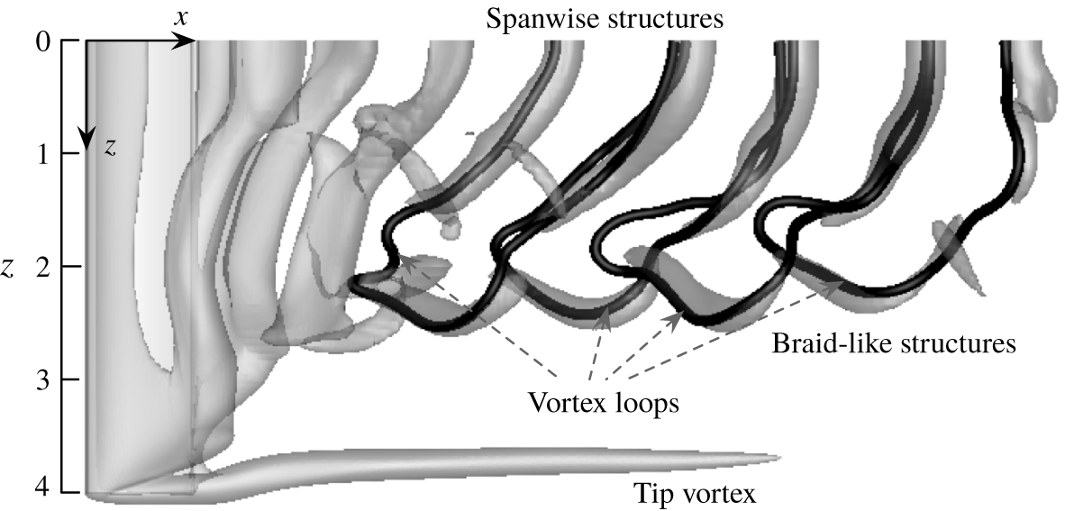
Top view of the wake for the case of  $(\unicode[STIX]{x1D6FC},sAR)=(22^{\circ },4)$. The black lines represent the vorticity lines. Isosurfaces of
 $Q=1$ are shown in transparent grey.

3.2 Three-dimensional wake structures
3.2.1 An overview of the vortical structures
Let us continue to examine the three-dimensional wake structures for the representative case of  $(\unicode[STIX]{x1D6FC},sAR)=(22^{\circ },4)$. A top view of the wake vortical structures is shown in figure 8. As also seen in figure 5, the wake can be divided into the tip vortex region at the free end and the unsteady vortex shedding region near the midspan. The tip vortex appears practically steady over time in the current case. The unsteadiness in the tip vortex becomes noticeable for cases with smaller
 $sAR$ and larger
 $\unicode[STIX]{x1D6FC}$, as discussed later in §§ 3.2.2 and 3.2.3. The unsteady region of the wake can be further divided into two subregions. Adjacent to the midspan (
 $z\lesssim 1.5$), the wake is dominated by vortex cores that are aligned predominantly with the spanwise direction. These vortices are formed by the roll-up of the vortex sheets from the leading and trailing edges, and shed alternatingly into the wake. On the other hand, the shedding vortices at
 $2\lesssim z\lesssim 2.5$ feature braid-like structures. These vortical structures are comprised of streamwise vorticity
 $\unicode[STIX]{x1D714}_{x}$ and cross-flow vorticity
 $\unicode[STIX]{x1D714}_{y}$, and are aligned mostly perpendicular to the spanwise direction. These vortical structures shed at the same frequency with the spanwise vortices.
The complex vortical structures in the unsteady region can be better understood by visualizing the vorticity lines, as depicted by the black solid lines in figure 8. Each vortex core in the braid-like region connects with a pair of counter-rotating spanwise vortical structures. These structures together form a closed vortex loop (considering the symmetry boundary condition at the midspan). The unsteady wake region is constituted of a series of such vortex loops arranged in a zigzag manner. It is thus clear that the braid-like structures play the role of closing the spanwise vortex system. This is in accordance with Helmholtz’s second law (Helmholtz Reference Helmholtz1858) which states that a vortex filament cannot terminate in a fluid (Batchelor Reference Batchelor1967). Similar vortex line models have also been proposed to describe the wakes of finite-span circular cylinders (Taneda Reference Taneda1952; Levold Reference Levold2012).
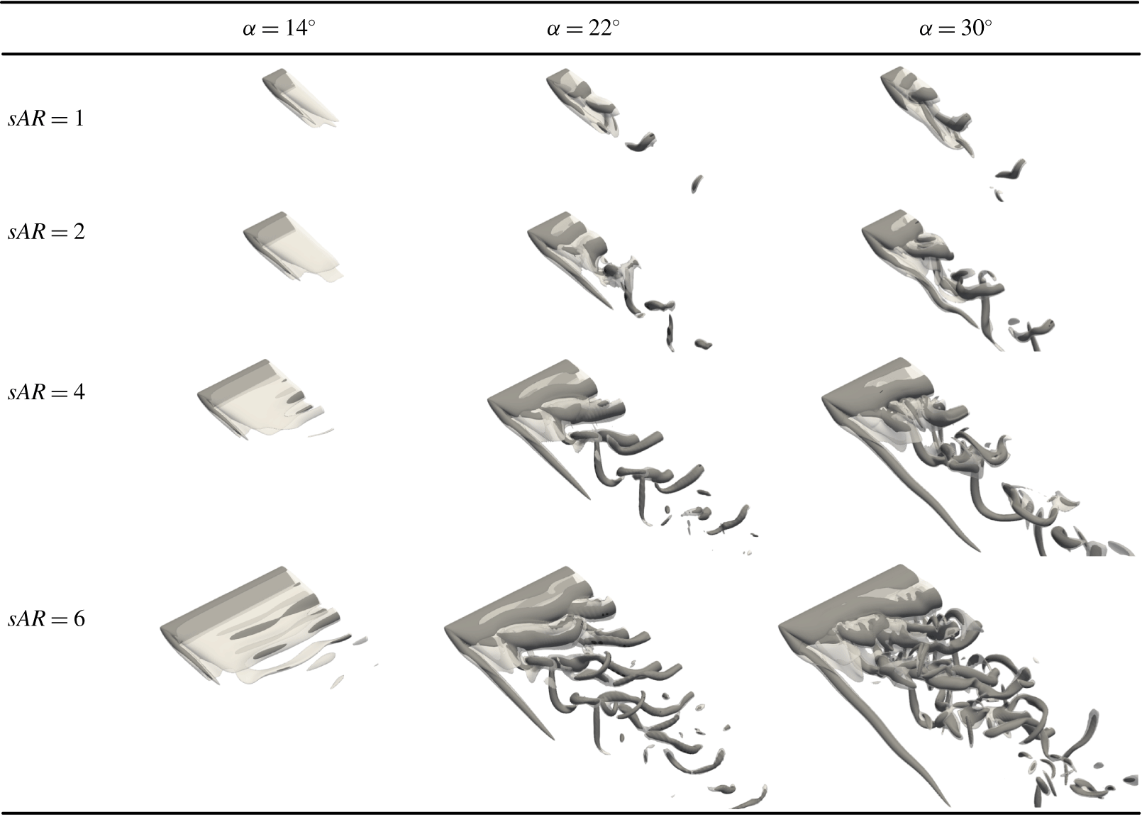
Perspective views of the wake vortices behind the finite wings with  $sAR=1$, 2, 4 and 6,
 $\unicode[STIX]{x1D6FC}=14^{\circ }$,
 $22^{\circ }$ and
 $30^{\circ }$. Vortical structures are visualized by the isosurfaces of
 $\Vert \unicode[STIX]{x1D74E}\Vert =2$ in light grey and
 $Q=1$ in dark grey.

3.2.2 Effects of  $sAR$ and $\unicode[STIX]{x1D6FC}$ on the wake


Separated flows behind finite-aspect-ratio wings are strongly influenced by the aspect ratio  $sAR$ and the angle of attack
 $\unicode[STIX]{x1D6FC}$. Let us show some representative wakes for a range of aspect ratios and angles of attack in figure 9. The short wings with
 $sAR=1$ generate different wake features compared with those discussed in § 3.2.1. Stable three-dimensional flow is observed at
 $\unicode[STIX]{x1D6FC}=14^{\circ }$, while the analogous two-dimensional flow at the same angle of attack exhibits periodic unsteady shedding. This indicates again that the tip effects stabilize the local flow, which in the current case of
 $sAR=1$ is the entire span. As the angle of attack is increased to
 $22^{\circ }$ and
 $30^{\circ }$, the wake instability becomes sufficiently strong to overcome the stabilizing effect from the tip, resulting in periodic shedding of the wake vortices. Originated from the leading edge with predominately spanwise vorticity, the shedding vortices on the suction side gradually morph into the hairpin vortices with their legs extending far upstream. The tip vortex cannot be clearly observed due to its strong interaction with the unsteady shedding vortices. Similar vortical features have also been reported in the wake of a flat-plate wing at similar Reynolds numbers by Taira & Colonius (Reference Taira and Colonius2009).
For  $sAR=2$, the increased spanwise extent alleviates the strong interaction between the tip vortex and unsteady shedding vortices as the case in
 $sAR=1$ wing. This enables the tip vortex to remain relatively steady despite the unsteadiness presented in the rest of the flow. The wake at
 $\unicode[STIX]{x1D6FC}=14^{\circ }$ exhibits weak periodic shedding according to a close examination of the lift force, although it may not be clearly visible in figure 9. At
 $\unicode[STIX]{x1D6FC}=22^{\circ }$, the unsteady shedding vortices mainly take the form of the braid-like structures, without clear spanwise vortex cores. As the angle of attack further increases to
 $\unicode[STIX]{x1D6FC}=30^{\circ }$, the unsteady vortex shedding grows stronger. Under its effect, the tip vortex exhibits noticeable undulations along the streamwise direction.
Increasing the aspect ratio to  $sAR=4$ reveals the spanwise vortex shedding region. The spanwise vortical structures are quite weak at
 $\unicode[STIX]{x1D6FC}=14^{\circ }$ and appear only in the direct vicinity of the midspan. With the increase in angle of attack, the unsteady shedding vortices grow stronger and extend farther into the wake. The tip vortex elongates compared with that at lower angles of attack. At
 $\unicode[STIX]{x1D6FC}=30^{\circ }$, small-scale streamwise vortical structures emerge in the spanwise shedding region, making the wake complex. The streamwise undulations in the tip vortex become less significant compared with that in the case of
 $(\unicode[STIX]{x1D6FC},sAR)=(30^{\circ },2)$.
As we consider a higher aspect ratio of 6, the spanwise shedding takes place over an expanded region for  $\unicode[STIX]{x1D6FC}=14^{\circ }$ and
 $22^{\circ }$. An additional feature that becomes clear at such high aspect ratio is the vortex dislocation, which divides the spanwise shedding region into two parts. This phenomenon is responsible for the low-frequency beating in the lift coefficients as shown in figure 2, and will be examined in detail in § 3.3. At
 $\unicode[STIX]{x1D6FC}=30^{\circ }$, smaller-scale streamwise vortical structures reminiscent of those induced by the Floquet instability (Deng, Sun & Shao Reference Deng, Sun and Shao2017; He et al. Reference He, Gioria, Pérez and Theofilis2017a) develop in the wake, making the unsteady shedding region even more complex.
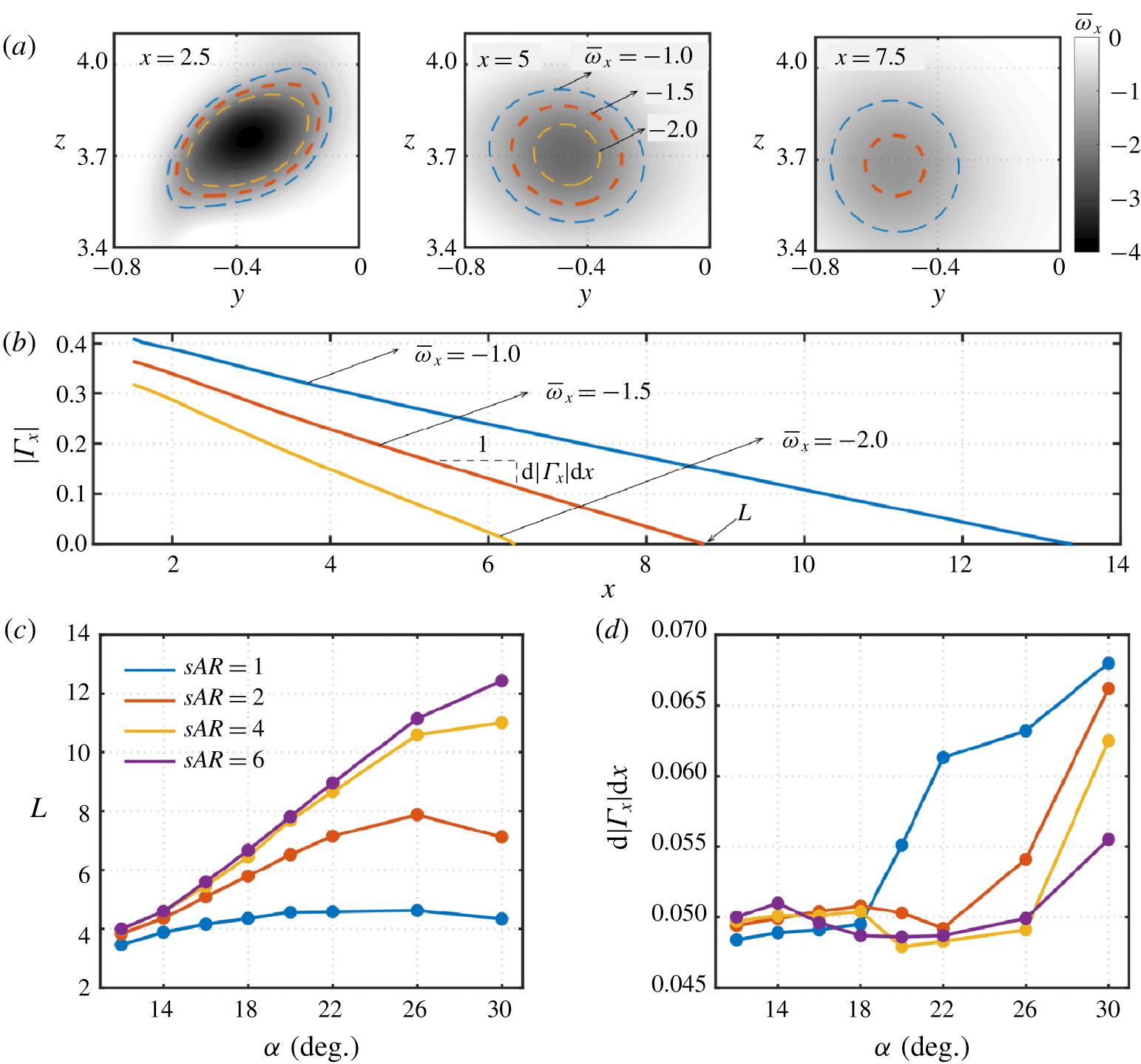
(a) Time-averaged streamwise vorticity fields at three streamwise locations of  $x=2.5$, 5 and 7.5 for
 $(\unicode[STIX]{x1D6FC},sAR)=(22^{\circ },4)$. The three dashed lines are the contour lines of
 $\overline{\unicode[STIX]{x1D714}}_{x}=-1.0$,
 $-1.5$ and
 $-2.0$. (b) Circulations based on the three contour lines. (c) Length
 $L$ of the tip vortex defined based on the zero-crossing point of
 $|\unicode[STIX]{x1D6E4}_{x}|$–
 $x$ line (
 $\unicode[STIX]{x1D6E4}_{x}$ evaluated based on contour of
 $\overline{\unicode[STIX]{x1D714}}_{x}=-1.5$), and (d) decay rate
 $\text{d}|\unicode[STIX]{x1D6E4}_{x}|/\text{d}x$.

3.2.3 Characteristics of the tip vortex
We characterize the tip vortex in detail here for the representative case of  $(\unicode[STIX]{x1D6FC},sAR)=(22^{\circ },4)$. The time-averaged streamwise vorticity fields in the tip region are shown in figure 10(a) at
 $x=2.5$, 5 and 7.5. The contours of
 $\overline{\unicode[STIX]{x1D714}}_{x}=-1.0$,
 $-1.5$ and
 $-2.0$ are shown to capture the shape of the vortex core. At
 $x=2.5$, the three contour lines are close to each other, depicting a mango-like shape. At
 $x=5$, the regions enclosed by the contours of
 $\overline{\unicode[STIX]{x1D714}}_{x}=-1.5$ and
 $-2.0$ shrink significantly. The vorticity level inside the vortex core also decreases. Further downstream at
 $x=7.5$, the tip vortex core becomes more diffused, and its shape relaxes to a circle.
The strength of the tip vortex can be quantitatively assessed through its streamwise circulation  $\unicode[STIX]{x1D6E4}_{x}=\oint _{C}\boldsymbol{u}\boldsymbol{\cdot }\,\text{d}\boldsymbol{l}$, where the integration contour
 $C$ is taken as one of the three contours shown in figure 10(a). Evaluating the circulations along the streamwise direction, we obtain three
 $|\unicode[STIX]{x1D6E4}_{x}|$-
 $x$ profiles in figure 10(b). With increasing streamwise distance, the contour
 $C$ shrinks, and the vortex diffuses. Both factors contribute to the decay of the strength of tip vortices in a linear manner with increasing streamwise distance. Such linear decay of the tip vortices has also been observed in Edstrand et al. (Reference Edstrand, Sun, Schmid, Taira and Cattafesta2018b). The line associated with smaller contour level
 $|\overline{\unicode[STIX]{x1D714}}_{x}|$ measures extended length and reduced decay rate.
To characterize the strengths of the tip vortices, we use the contour of  $\overline{\unicode[STIX]{x1D714}}_{x}=-1.5$ and calculate the length
 $L$ and the decay rate
 $\text{d}|\unicode[STIX]{x1D6E4}_{x}|/\text{d}x$ for different cases, as summarized in figures 10(c) and 10(d). We show in the Appendix that the choice of the contour level does not affect the insights drawn here. For the majority of the cases (
 $sAR\geqslant 2$,
 $\unicode[STIX]{x1D6FC}\leqslant 26^{\circ }$), the length of the tip vortex increases almost linearly with the angle of attack. The decay rate remains mostly constant at
 $\text{d}|\unicode[STIX]{x1D6E4}_{x}|/\text{d}x\approx 0.05$ due to viscous diffusion. Significant increase of the decay rate is observed at
 $\unicode[STIX]{x1D6FC}\approx 26^{\circ }{-}30^{\circ }$ with
 $sAR\gtrsim 2$ and
 $\unicode[STIX]{x1D6FC}\gtrsim 20^{\circ }$ with
 $sAR=1$. In these cases, the strong wake vortex shedding induces unsteady motion of the tip vortex, as observed in figure 9. This unsteadiness serves as an additional mechanism (to diffusion) to reduce the time-averaged strength of the tip vortex. As a result, the
 $L{-}\unicode[STIX]{x1D6FC}$ relationship as shown in figure 10(c) no longer follows the linear growth as at smaller
 $\unicode[STIX]{x1D6FC}$. At
 $sAR=1$ and 2, the time-averaged tip vortex length appears to even decrease at large angles of attack.
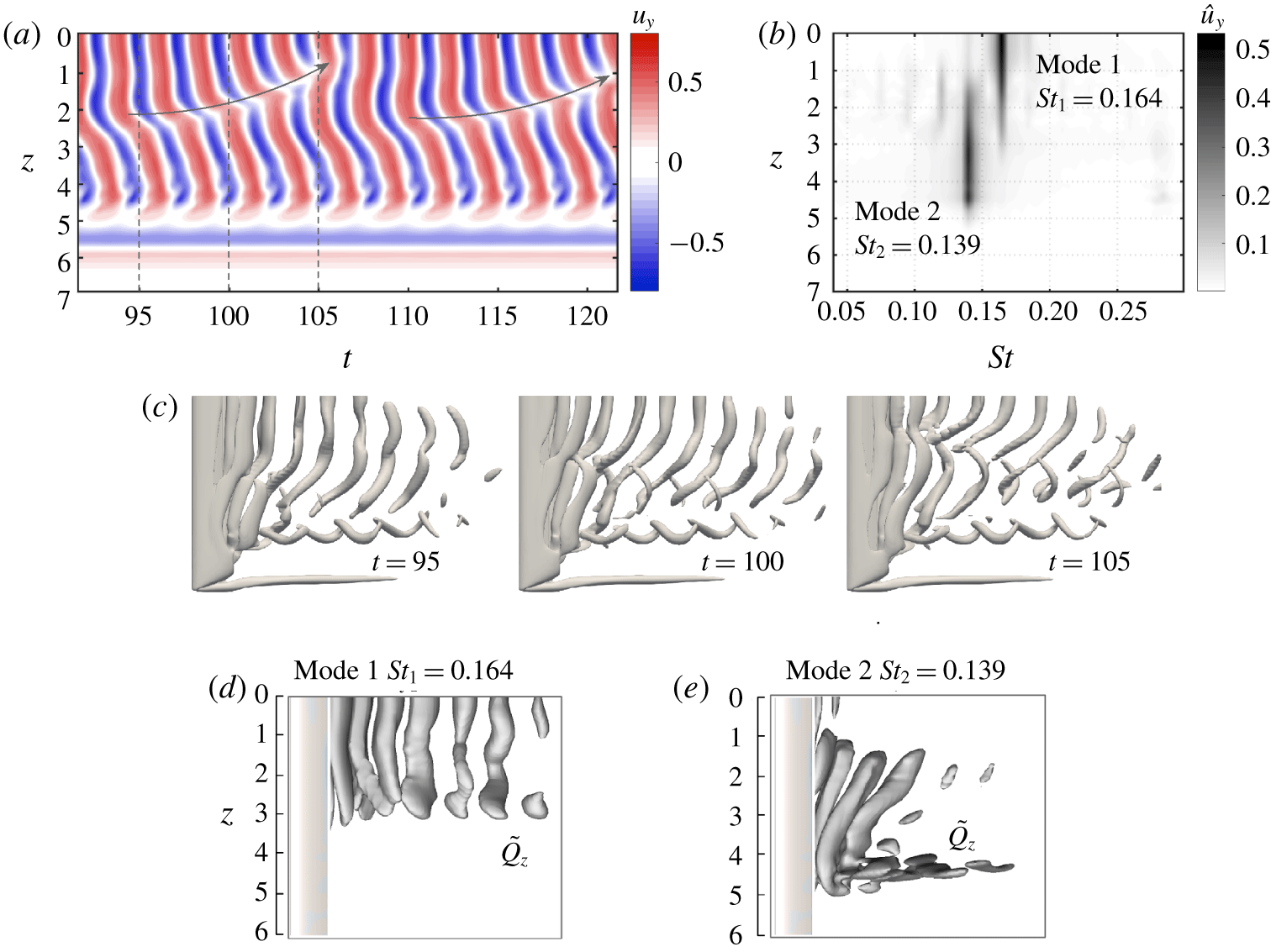
(a) Spatial-temporal distribution of the cross-flow velocity probed at  $(x,y)=(2,-0.3)$ for the case
 $(\unicode[STIX]{x1D6FC},sAR)=(22^{\circ },6)$. The grey arrow indicates the translating direction of the vortex dislocation. (b) Frequency distribution of the velocity over the spanwise direction. (c) Isosurfaces of
 $Q=1$ at three time instances showing one cycle of vortex dislocation. (d,e) The DMD (dynamic mode decomposition) modes (
 $Q$ criteria) for the two identified frequencies.

3.3 Spectral analysis of vortex dislocation
As discussed in § 3.2.2, for large-aspect-ratio wings, vortex dislocation occurs, dividing the spanwise vortex shedding region. Here, we focus on the particular case of  $(\unicode[STIX]{x1D6FC},AR)=(22^{\circ },6)$. The cross-flow velocity
 $u_{y}$ along
 $(x,y,z)=(2,-0.3,0-7)$ over time is presented in figure 11(a). For
 $z\gtrsim 5$, which corresponds to the tip vortex region, the velocity remains steady over time. For
 $0\leqslant z\lesssim 5$, the variations in the velocity indicate the occurrence of the periodic vortex shedding. Along with the vortical structures in figure 9 for
 $(\unicode[STIX]{x1D6FC},sAR)=(22^{\circ },6)$, vortex dislocation is clearly observed from the discontinuities in the spanwise vortices. With the point of dislocation translating repeatedly from
 $z\approx 3.5$ to
 $z\approx 1$, the wake also changes over time, as observed from the isosurfaces of
 $Q=1$ in figure 11(c). At
 $t=95$, the spanwise vortical structures appear intact. Around
 $t=100$, vortex dislocation starts to develop in the near wake. By
 $t=105$, the formation of two shedding cells are clearly visible.
To gain additional insights, we apply a Fourier transform to the cross-flow velocity  $u_{y}$ at each spanwise section, as shown in figure 11(b). We use
 $\hat{u} _{y}$ to denote the power spectral density (PSD) of the velocity fluctuation. The two spanwise shedding structures are found to be associated with different frequencies. The structures closer to the midspan shed with a frequency of
 $St_{1}=0.164$ (
 $St\equiv fc\sin \unicode[STIX]{x1D6FC}/U_{\infty }$, where
 $f$ is the dimensional shedding frequency). On the other hand, the structures closer to the wing tip shed with a lower frequency of
 $St_{2}=0.139$. For the current case, the point of dislocation translates along the wing span periodically from
 $z\approx 1$ to 3, at the beating frequency
 $St_{1}-St_{2}$. To identify the vortical structures associated with these two frequencies, we perform dynamic mode decomposition (Rowley et al. Reference Rowley, Mezić, Bagheri, Schlatter and Henningson2009; Schmid Reference Schmid2010) on the
 $Q$ criteria. As shown in figure 11(d), the modal structures corresponding to
 $St_{1}$ is composed of the columnar vortex cores aligned with the spanwise direction. In contrast, the mode with frequency
 $St_{2}$ presents three-dimensional modal structures comprised of skewed vortex cores as well as the streamwise vortical structures. These two modes overlap over
 $1\lesssim z\lesssim 3$. As time evolves, the time-varying phase between these two modes results in the changes in the vortical structures, as observed in figure 11(c).
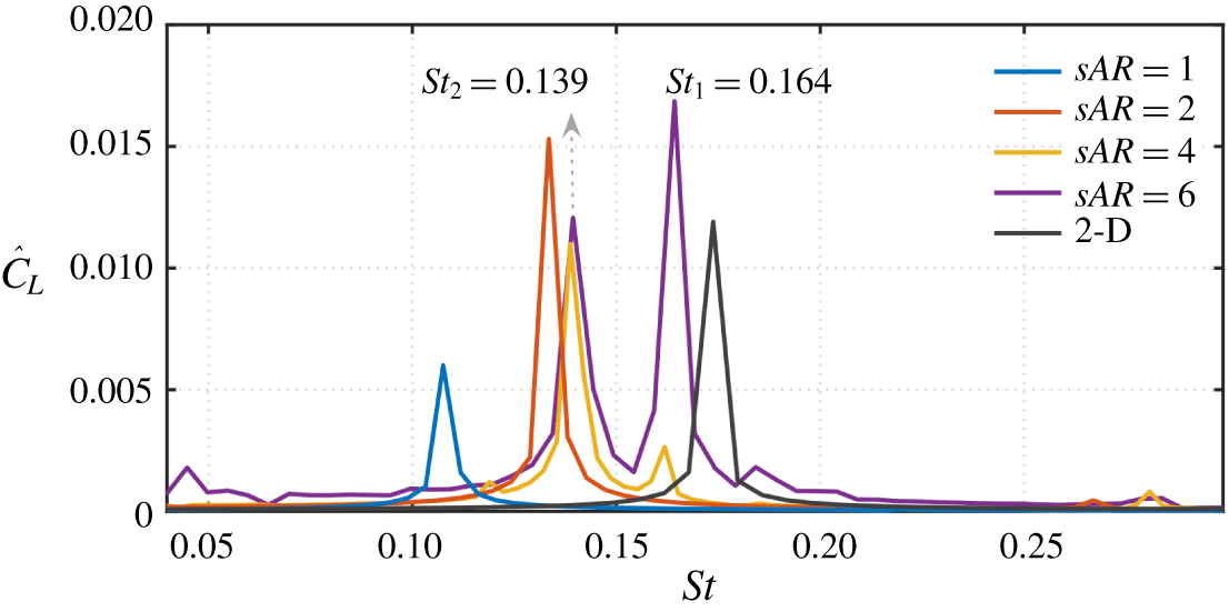
Frequency spectra of lift coefficients at  $\unicode[STIX]{x1D6FC}=22^{\circ }$ for different aspect ratios. Here,
 ${\hat{C}}_{L}$ denotes the PSD of the lift coefficient. The PSD of the two-dimensional case is scaled down by a factor of 10 for visual clarity.

The dominant frequencies identified in the wake for  $(\unicode[STIX]{x1D6FC},sAR)=(22^{\circ },6)$ are also detected in the corresponding lift spectrum, as shown in figure 12. Also overlaid are the lift spectra for other aspect ratios with
 $\unicode[STIX]{x1D6FC}=22^{\circ }$. The two-dimensional airfoil sheds vortices at the frequency of
 $St=0.174$, which is close to that reported by Rojratsirikul et al. (Reference Rojratsirikul, Genc, Wang and Gursul2011) and Calderon, Wang & Gursul (Reference Calderon, Wang and Gursul2013), regardless of the big difference in Reynolds numbers (the cited works cover
 $Re=10\,000{-}50\,000$). The dominant frequency
 $St_{1}$ for
 $sAR=6$ is close to the frequency in the two-dimensional case. This suggests the two-dimensional nature of the corresponding modal structure (mode 1) as shown in figure 11(d). On the other hand,
 $St_{2}$ almost coincides with the primary frequency in the cases of
 $sAR=2$ and 4, hinting that the lower shedding frequency is caused by the slowdown of shedding from the tip effects. The downward induced velocity from the tip vortex slows the shedding of the neighbouring vortical structures. For the much lower
 $sAR=1$ case, the strong interaction between the tip vortex and the unsteady vortices further slows down the vortex shedding, resulting in a lower shedding frequency. It should be noted that such a large influence of aspect ratio on Strouhal number is not observed at higher Reynolds numbers, at which the aspect ratio has a remarkably small effect on the shedding frequency, as reported by Rojratsirikul et al. (Reference Rojratsirikul, Genc, Wang and Gursul2011) and Calderon et al. (Reference Calderon, Wang and Gursul2013).
The lift spectra for different  $sAR$ reveal how the tip effects influence the wake dynamics along the span. For
 $sAR\lesssim 4$, the tip effects dominate over the whole span of the wing, as discussed in §§ 3.2.1 and 3.2.2. For a higher aspect ratio, the tip effects become weaker over the extended region of
 $z\gtrsim 4$. This allows nominally two-dimensional structures to develop near the midspan and compete with the three-dimensional shedding near the tip, giving rise to vortex dislocation. Based on the insights obtained from spectral analysis, we are able to identify mainly three wake regions along the spanwise direction for large-aspect-ratio wings: (i) the tip vortex region as a direct consequence of the wing tip, (ii) the nominally two-dimensional shedding region near the midspan (mode 1) where the influence of the tip vortex is weak, and (iii) the three-dimensional shedding region (mode 2) that are influenced by the interaction between regions (i) and (ii).
3.4 Classification of the wake
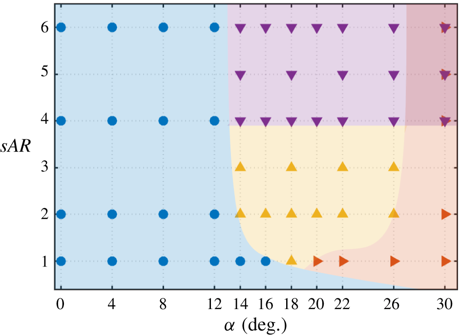
We summarize our wake characterization over aspect ratio and angle of attack in figure 13. At  $Re=400$, the wake remains stable for
 $\unicode[STIX]{x1D6FC}\lesssim 12^{\circ }$ for the aspect ratios considered in this study. For
 $sAR=1$, the flow can remain steady for even a higher angle of attack of
 $\unicode[STIX]{x1D6FC}=16^{\circ }$ due to the stabilizing tip effects. We shade in blue the conditions for a stable wake in figure 13. The transition from steady to unsteady flow is attributed to the Hopf bifurcation associated with the periodically shedding vortical structures (Ahuja et al. Reference Ahuja, Rowley, Kevrekidis, Wei, Colonius and Tadmor2007; Taira & Colonius Reference Taira and Colonius2009).
Classification of the wake. ●, stable flow; ▴, steady tip vortex and unsteady shedding vortices; ▸, unsteady tip vortex; ▾, vortex dislocation.

With the increase in angle of attack, the vortex sheet generated from the leading and trailing edges form shedding vortices, as highlighted by the yellow region in figure 13. At this stage, the downwash provided by the tip vortex is no longer able to keep these wake vortices stationary. The wake here is characterized by the presence of two types of vortices: the unsteady shedding vortices and the tip vortex. The unsteady vortices take the form of spanwise vortex cores with their braid-like structures forming closed loops as described in § 3.2.1.
For higher-aspect-ratio wings, the unsteady wake exhibits an additional feature of vortex dislocation. With the tip vortex imposing downwash on the shedding vortices near the tip, their shedding frequency becomes lower than that of the shedding structures over the midspan region. When the discrepancy between these two frequencies become significant, the spanwise shedding processes become desynchronized, resulting in vortex dislocation as shown in figure 11(b). This phenomenon (shaded in purple) is observed for  $sAR\gtrsim 4$ regardless of angle of attack, as long as
 $\unicode[STIX]{x1D6FC}$ is large enough to trigger vortex shedding. This type of vortex dislocation is ubiquitous for bluff body flows with spanwise inhomogeneity (Eisenlohr & Eckelmann Reference Eisenlohr and Eckelmann1989; Williamson Reference Williamson1989; Noack, Ohle & Eckelmann Reference Noack, Ohle and Eckelmann1991; Techet, Hover & Triantafyllou Reference Techet, Hover and Triantafyllou1998; Lucor, Imas & Karniadakis Reference Lucor, Imas and Karniadakis2001).
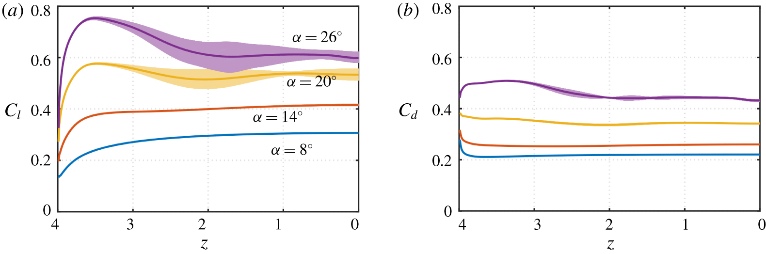
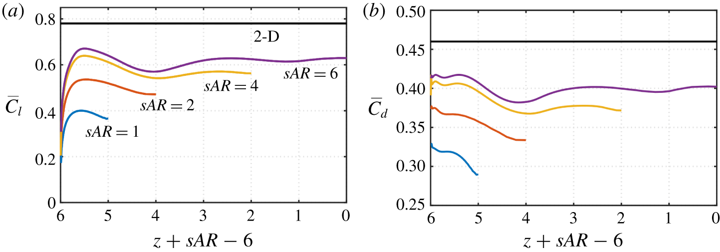
Sectional (a) lift coefficients and (b) drag coefficients for  $sAR=4$ with varying angles of attack. The thick curves represent the time-averaged values and the shaded regions represent their temporal fluctuations.

As we consider higher angles of attack, the tip vortex exhibits noticeable undulation in the streamwise direction due to its strong interaction with the unsteady shedding vortices. Such cases are observed over the red region in figure 13. We note that in realistic flows without the prescribed slip boundary condition at midspan, these flows might become asymmetric with respect to the midspan, as analysed in Taira & Colonius (Reference Taira and Colonius2009). We notice that the transition curve separating the unsteady tip vortex region from the yellow and purple regions is similar to the periodic/aperiodic transition in Taira & Colonius (Reference Taira and Colonius2009). This might suggest that the strong interaction between the tip vortices and the unsteady shedding vortices provides a route for the flow to transition to an asymmetric wake, if the symmetry plane is removed. Such transition is likely caused by the out-of-phase oscillations of the tip vortices at the two ends of the full wing. An unsteady tip vortex can also interact with the spanwise vortices experiencing vortex dislocation to create a complex wake as indicated by the top right subregion of figure 13. This complex wake generates finer-scale vortical structures from the rich interactions among the tip vortices and the large shedding vortices.
3.5 Aerodynamic forces
The three-dimensional wake imposes spanwise variations in the sectional distributions of the forces on the wing. The sectional lift and drag forces for  $sAR=4$ are presented for various angles of attack in figure 14. For the cases of
 $\unicode[STIX]{x1D6FC}=8^{\circ }$ and
 $14^{\circ }$,
 $C_{l}$ gradually decreases from the midspan to the wing tip. The drag coefficient remains almost constant over the majority of the span except for the slight increase at the wing tip.
For angles of attack above  $20^{\circ }$, considerable temporal fluctuations of
 $C_{l}$ appear in the unsteady shedding region, especially near
 $z\approx 2$. The temporal fluctuations in the drag coefficients are significantly lower than the lift coefficients. As the flow becomes steady towards the wing tip region, the temporal fluctuation of
 $C_{l}$ gradually disappears. We note here that the time-averaged sectional
 $\overline{C_{l}}$ exhibits a peak at
 $z\approx 3.5$ before it drastically drops at the wing tip. This is in contrast to the cases with lower angles of attack, where
 $C_{l}$ decays monotonically towards the tip. This difference in the lift profile will be related to the difference in the near-tip vortical structures in the discussion below.
Let us now resort to the force element theory (Chang Reference Chang1992; Lee et al. Reference Lee, Hsieh, Chang and Chu2012) to identify the wake structures that exert aerodynamic forces on the wing. In this theory, we utilize an auxiliary potential  $\unicode[STIX]{x1D719}_{L}$ (take the lift force for example) that satisfies the boundary condition
 $-\boldsymbol{n}\boldsymbol{\cdot }\unicode[STIX]{x1D735}\unicode[STIX]{x1D719}_{L}=\boldsymbol{n}\boldsymbol{\cdot }\boldsymbol{e}_{\boldsymbol{y}}$. By taking the inner product of the Navier–Stokes equation (2.1b) with the potential velocity
 $\unicode[STIX]{x1D735}\unicode[STIX]{x1D719}_{L}$ and integrating over the entire fluid domain
 $V$, the pressure force term
 $\int _{S}p\boldsymbol{n}\boldsymbol{\cdot }\boldsymbol{e}_{\boldsymbol{y}}\,\text{d}S$ in (2.2) can be expressed as a volume integration of wake variables and a surface integration. The lift force can then be expressed as
 $$\begin{eqnarray}F_{L}=\int _{V}\unicode[STIX]{x1D74E}\times \boldsymbol{u}\boldsymbol{\cdot }\unicode[STIX]{x1D735}\unicode[STIX]{x1D719}_{L}\,\text{d}V+\frac{1}{Re}\int _{S}\unicode[STIX]{x1D74E}\times \boldsymbol{n}\boldsymbol{\cdot }(\unicode[STIX]{x1D735}\unicode[STIX]{x1D719}_{L}+\boldsymbol{e}_{\boldsymbol{y}})\,\text{d}S.\end{eqnarray}$$
The integrands in the first and second terms on the right-hand side are called the volume lift and the surface lift elements, respectively. The drag force elements can be obtained in a similar fashion by replacing the velocity potential  $\unicode[STIX]{x1D719}_{L}$ with
 $\unicode[STIX]{x1D719}_{D}$ and enforcing
 $-\boldsymbol{n}\boldsymbol{\cdot }\unicode[STIX]{x1D735}\unicode[STIX]{x1D719}_{D}=\boldsymbol{n}\boldsymbol{\cdot }\boldsymbol{e}_{\boldsymbol{x}}$ on the wing surface.
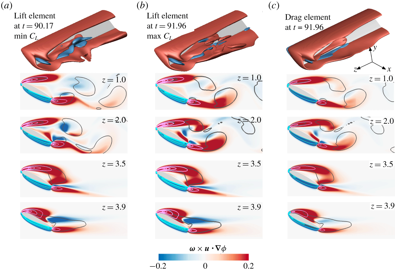
Volume force elements for  $(\unicode[STIX]{x1D6FC},sAR)=(26^{\circ },4)$. (a) Lift elements at
 $t=90.17$ at which
 $C_{L}$ is the lowest. (b) Lift force element at
 $t=91.60$ at which
 $C_{L}$ is the highest. (c) Drag force element at
 $t=91.60$. In the top row, the isosurfaces of lift or drag force elements are shown with the contour level of
 $\pm 0.2$. The two-dimensional contour plots show the force elements at indicated
 $z$ planes with the black contours representing the vortex cores (
 $Q=1$). The magenta solid lines represent contours of positive force elements starting from
 $\unicode[STIX]{x1D74E}\times \boldsymbol{u}\boldsymbol{\cdot }\unicode[STIX]{x1D735}\unicode[STIX]{x1D719}=1$ (outmost contour) with an increment of 2 towards the inside, and the cyan solid lines are the contours of negative force elements starting from
 $\unicode[STIX]{x1D74E}\times \boldsymbol{u}\boldsymbol{\cdot }\unicode[STIX]{x1D735}\unicode[STIX]{x1D719}=-1$ (outmost) with an interval of
 $-2$.

Isosurfaces of  $\overline{Q}=3$ for an
 $sAR=4$ wing and varying angles of attack.

The lift elements for the case of  $(\unicode[STIX]{x1D6FC},sAR)=(26^{\circ },4)$ at two time instances, at which the instantaneous lift coefficient is lowest and highest, are shown in figures 15(a) and (b), respectively. In the current study, the contribution of the viscous surface lift element is below 15 % of the total force. For this reason, we only report below the dominant volume lift element
 $\unicode[STIX]{x1D74E}\times \boldsymbol{u}\boldsymbol{\cdot }\unicode[STIX]{x1D735}\unicode[STIX]{x1D719}_{L}$. Due to the spatially compact nature of the auxiliary potential gradient
 $\unicode[STIX]{x1D735}\unicode[STIX]{x1D719}_{L}$, high levels of lift elements are concentrated in the vicinity of the wing. The two free shear layers emanating from both the suction and pressure sides contribute positively to lift, whereas the boundary layer on the pressure surface contributes adversely to the total lift. Similar observations have also been reported on an impulsively started finite-plate wing by Lee et al. (Reference Lee, Hsieh, Chang and Chu2012).
Comparing the snapshots between two time instances, the difference is observed in the unsteady shedding region. The difference in the lift elements between the two time instances at  $z=1$ is subtle. However, at
 $z=2$, significant amounts of negative lift elements appear in figure 15(a) and disappear in figure 15(b). This explains the larger lift fluctuations at
 $z\approx 2$ than the other regions, as observed in figure 14(a).
Near the tip at  $z=3.5$, the local flow is steady and the distributions of lift elements at two time instants are indistinguishable from each other. Noteworthy here is the large distribution of positive lift element near the wing tip giving rise to an increase of sectional lift at around
 $z=3.5$ in figure 14. Inward from the tip vortex is a vortical structure that forms by rolling up the leading-edge vortex sheet, which is seen from figure 16 for higher angles of attack. This also explains the absence of such local lift increase at lower angles of attack, as the rolled-up vortical structure from the leading edge does not form next to the tip vortex. Such local lift enhancement due to the downwash of tip vortices has also been discussed at length by DeVoria & Mohseni (Reference DeVoria and Mohseni2017) for steadily translating wings at high angles of attack.
Farther towards the tip at  $z=3.9$, negative lift elements emerge in the near wake and the positive lift elements diminish, giving rise to the drastic drop in the sectional lift force. It is noteworthy that the trailing part of the tip vortex barely contributes to the aerodynamic forces. This is not only because of the fast decay of the velocity potential
 $\unicode[STIX]{x1D735}\unicode[STIX]{x1D719}_{L}$, but also due to the fact that in the core of the tip vortex, the velocity vector and the vorticity vector are both aligned with the streamwise direction. The cross product
 $\unicode[STIX]{x1D74E}\times \boldsymbol{u}$ is small in magnitude, thus making the integrand in (3.2) negligible.
The volume drag elements for the same case are shown in figure 15(c). In general, the drag elements share similar patterns with that of the lift elements, where the two separated free shear layers contribute positively to the total drag and the boundary layer on the pressure side contributes negatively. The isosurfaces of drag elements, compared with the lift element at the same time instances, are devoid of the small-scale structures. Moreover, the intensity of the drag elements is lower compared to the lift elements, as judged from the absence of high-level contour lines of the drag elements. Thus, the integrated drag is smaller than lift in both temporal fluctuations as well as time-averaged value, as depicted in figure 14.
Influence of aspect ratio on the sectional (a) lift and (b) drag coefficients at  $\unicode[STIX]{x1D6FC}=22^{\circ }$. The force coefficients are aligned from the wing tip.

We further examine the effect of aspect ratio on the sectional lift coefficients for  $\unicode[STIX]{x1D6FC}=22^{\circ }$ in figure 17. Here, the force coefficients are presented by aligning the distributions from the wing tip. With the increase in
 $sAR$, the lift coefficients increase, although they remain below the two-dimensional lift value at the same angle of attack. Focusing on the tip region, the peak in sectional lift near the tip is observed for finite-aspect-ratio wings. This is caused by the presence of the leading-edge vortical structure near the tip as discussed above. Such a structure gives rise to the increase in lift approximately 0.3–0.4 chords away from the tip. Similar to the lift coefficients, the drag coefficients increase with aspect ratio. However, the spanwise variations for the drag coefficients are relatively small compared to lift. The increase of the sectional
 $\overline{C_{d}}$ near the tip is also observed for all aspect ratios at the angle of attack of
 $\unicode[STIX]{x1D6FC}=22^{\circ }$.
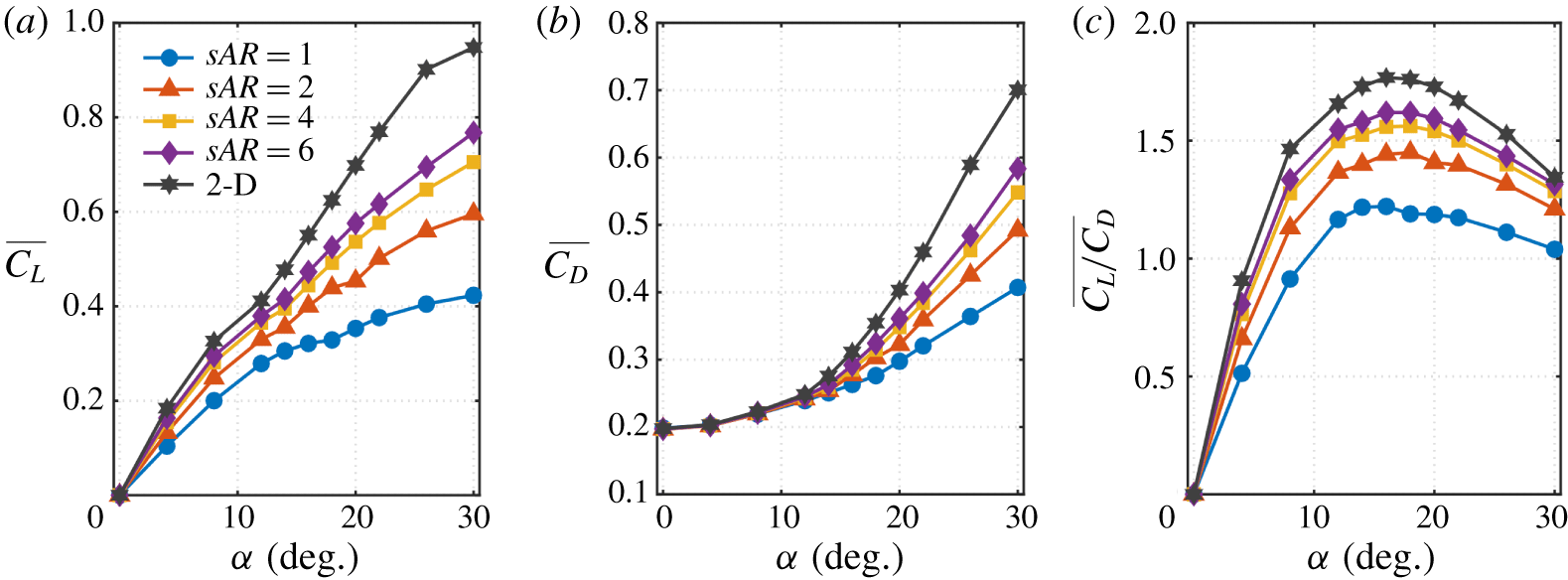
Time-averaged (a) lift coefficient, (b) drag coefficient and (c) lift-to-drag ratio.

At last, let us summarize our aerodynamic force data for the finite-aspect-ratio wings. The time-averaged lift coefficients  $\overline{C_{L}}$, drag coefficients
 $\overline{C_{D}}$ and the lift-to-drag ratios
 $\overline{C_{L}/C_{D}}$ are plotted in figure 18. Overall, we notice that the lift and drag coefficients on the wing are smaller for lower-aspect-ratio wings and tend toward the two-dimensional limit for higher-aspect-ratio wings.
For the lift coefficients shown in figure 18(a), we observe that the tip effects reduce lift even at low angles of attack. For post-stall flows, the influence of the tip vortices on lift becomes more noticeable with wider variations in the lift values with respect to  $sAR$. At a low Reynolds number of 400, lift coefficients monotonically increase for the range of angles of attack considered. The enhanced lift at higher angles of attack is created by the vortical structures that form above the wing as seen in figure 15 (Taira & Colonius Reference Taira and Colonius2009; Lee et al. Reference Lee, Hsieh, Chang and Chu2012). We can observe that above
 $\unicode[STIX]{x1D6FC}\approx 12^{\circ }$, there is a change in the lift slope which is caused by the emergence of unsteadiness in the wake, as shown in figure 13.
Next, let us examine the variation of drag coefficient over the angle of attack. As in the case with lift, we observe that the drag coefficients become higher as the aspect ratio increases. This is due to the flow being able to pass around the tip to reduce the drag coefficient for lower-aspect-ratio wings. However, we notice a striking feature that the drag coefficient is almost independent of the aspect ratio up to  $\unicode[STIX]{x1D6FC}\approx 12^{\circ }$. This suggests that the drag force is primarily due to viscous effects even though the flow is separated at the moderate angles of attack. Once the wake becomes unsteady beyond
 $\unicode[STIX]{x1D6FC}\approx 12^{\circ }$, pressure effects contribute significantly to drag, which then is influenced by the aspect ratio and the resulting unsteady wake profiles. These observations are also in agreement with the findings for finite-aspect-ratio flat-plate wings from Taira & Colonius (Reference Taira and Colonius2009).
At this low Reynolds number, the lift-to-drag ratio is limited to  $O(1)$, as evident from figure 18(c). Another unique feature for such low-
 $Re$ aerodynamics is the high angle of attack at which the peak lift-to-drag ratio is achieved. These ratios are generally in agreement with those for finite-
 $sAR$ flat-plate wings from (Taira & Colonius Reference Taira and Colonius2009), but achieve their peaks at slightly higher angles of attack for the NACA 0015 airfoil. Such observations are reported in Torres & Mueller (Reference Torres and Mueller2004) for a higher Reynolds number of
 $10^{5}$. If the finite wings are to be operated in steady condition, it can still achieve a high lift-to-drag ratio for
 $\unicode[STIX]{x1D6FC}\lesssim 12^{\circ }$. The ratio can be further increased but unsteadiness in the forces from the wake dynamics needs to be considered.
4 Conclusion
We performed direct numerical simulations of the flow over unswept NACA 0015 wings with straight cut tip at a Reynolds number of 400 with the objective of characterizing the tip effects on the three-dimensional separated flows. The present study considered a half-span wing model with symmetry boundary condition prescribed at the midspan. An extensive parametric study was performed for aspect ratios of  $sAR=1{-}6$ and angles of attack of
 $\unicode[STIX]{x1D6FC}=0^{\circ }{-}30^{\circ }$.
Based on these simulations, we have made several observations on the emergence of three-dimensional separation and wake patterns. The inception of three dimensionality is closely tied to the formation of the tip vortex. Vorticity is introduced to the flow from the wing surface in a predominantly two-dimensional manner. As the vortex sheet rolls up around the wing tip to form the tip vortex, three dimensionality is introduced to the flow but is confined to the near-tip region of the boundary layer. Once the tip vortex reaches its maturity, the stronger downwash influences the roll-up of the leading and trailing-edge vortex sheets, generating three-dimensional vortical structures in the wake and imposing a three-dimensional flow pattern in the vicinity of the wing surface.
The three-dimensional wake is dependent on the aspect ratio and angle of attack of the finite-aspect-ratio wing. For wings with low  $sAR$, the strong downwash from the tip vortex inhibits the roll-up of the leading and trailing-edge vortex sheets over the entire span. For this reason, the wake is able to remain steady for moderate angles of attack. For wings with higher
 $sAR$, the relatively weakened tip effects near the midspan are no longer able to keep the leading- and trailing-edge vortex sheets from rolling up. As a result, unsteady shedding takes place away from the tip. These shedding vortices are in the form of spanwise vortex cores and braid-like structures. Together they close the vortex loops as they shed into the wake. Further increasing the
 $sAR$ brings out the locally two-dimensional vortical structures at the midspan. Their competition with the near-tip three-dimensional shedding vortices results in vortex dislocation. For high angles of attack, the wake becomes complex with interactions among the wake vortices. With streamwise oscillations appearing at higher angles of attack, the wake may transition to asymmetric flow about the midspan in the absence of symmetry boundary condition. These wake features are mapped over a range of aspect ratio and angles of attack.
The three-dimensional wake dynamics has a significant impact on the sectional distribution of aerodynamics forces. By using the force element analysis, we identified the dominant vortical structures responsible for exerting lift and drag forces on the wing. Noteworthy here are the high sectional force coefficients near the tip for cases at high angles of attack. Such local increases in force coefficients are attributed to the stationary vortical structure formed inward from the tip vortex. From the simulations, the aerodynamic force coefficients and the lift-to-drag ratio were also summarized for a wide range of aspect ratios and angles of attack. Through a comprehensive analysis of the forces and wake dynamics, the relationship between the aspect ratio and the unsteadiness in the aerodynamic characteristics of the wing were revealed.
This study offers a detailed look into the influence of the tip effects on the formation of three-dimensional wake behind finite-aspect-ratio wings. The insights obtained from this study are critical for the understanding of the more complex wake flows at higher Reynolds number, as some of the coherent vortices at high  $Re$ share similar core structures with the analogous vortical wakes of low
 $Re$ flow. This is especially true for tip vortices that remain coherent across a wide range of Reynolds numbers. Moreover, the knowledge gained here can serve as an important reference to wings with unsteady manoeuvres, as well as to active flow control strategies to stabilize or take advantage of vortical forces.
Acknowledgements
We acknowledge the US Air Force Office of Scientific Research (program managers: Dr G. Abate and Dr D. Smith, grant no. FA9550-17-1-0222) for funding this project. We thank the anonymous referees for their valuable comments in improving this paper.
Declaration of interests
The authors report no conflict of interest.
Appendix. Effect of contour level on the characterization of the tip vortex
In § 3.2.3, the evaluation of the length  $L$ and decay rate
 $\text{d}|\unicode[STIX]{x1D6E4}_{x}|/\text{d}x$ of the tip vortex involves the selection of
 $\overline{\unicode[STIX]{x1D714}}_{x}$ contour level. We have selected
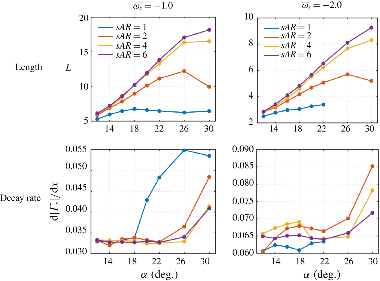
 $\overline{\unicode[STIX]{x1D714}}_{x}=-1.5$ as a representative contour level and compiled the characteristics of the tip vortex for various cases. Here, we examine two other contour levels to show that the overall findings are not influenced by the choice of contour level. The lengths and decay rates of the tip vortex based on
 $\overline{\unicode[STIX]{x1D714}}_{x}=-1.0$ and
 $-2.0$ are shown in figure 19. As qualitatively observed in figure 10(b), the absolute values of
 $L$ and
 $\text{d}|\unicode[STIX]{x1D6E4}_{x}|/\text{d}x$ are dependent on the choice of contour level. The larger the selected value of
 $|\overline{\unicode[STIX]{x1D714}}_{x}|$ is, the shorter the length and the larger the decay rate become. However, the variations of
 $L$ and
 $\text{d}|\unicode[STIX]{x1D6E4}_{x}|/\text{d}x$ with respect to
 $\unicode[STIX]{x1D6FC}$,
 $sAR$ and
 $Re$ within each contour level follow the same trends with those based on
 $\overline{\unicode[STIX]{x1D714}}_{x}=-1.5$. This suggests that the observations we have made in § 3.2.3 are independent of the choice of the contour level considered in the present study.
Effect of  $\overline{\unicode[STIX]{x1D714}}_{x}$ contour level on the length and decay rate of the tip vortex.