


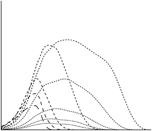





1. Introduction
The spectral theory of homogeneous turbulence without boundaries dates back a long way (see e.g. the book by Batchelor Reference Batchelor1953), while more recent studies have allowed for effects such as rotation and stratification which tend to produce anisotropy. The understanding of turbulence in the presence of rotation is a basic problem of fluid mechanics, whose applications include geophysical flows, turbomachinery and astrophysics. In the geophysical context, we refer the reader to the reviews by Moum (Reference Moum2021), Fritts & Alexander (Reference Fritts and Alexander2003), Kim, Eckermann & Chun (Reference Kim, Eckermann and Chun2003) and Thomas (Reference Thomas2023). We also refer the reader to the book by Sagaut & Cambon (Reference Sagaut and Cambon2018) for a wide-ranging discussion of work on homogeneous turbulence, in particular chapter 7, which concerns turbulence with rotation.
Among the many approaches which have previously been used to attack the problem of rotating turbulence, spectral closures bear a close relationship to the present work. In particular, the EDQNM (eddy damped quasi-Markovian) model has been the subject of articles by Cambon & Jacquin (Reference Cambon and Jacquin1989), Waleffe (Reference Waleffe1993) and Cambon, Mansour & Godeferd (Reference Cambon, Mansour and Godeferd1997). Direct numerical simulation (DNS) has also played an increasingly important role in recent years (see e.g. Teitelbaum & Mininni Reference Teitelbaum and Mininni2012 and references therein). However, we should note that estimates of the computational cost of credible DNS for the present problem suggest it is well out of reach of current computational resources for the parameter regimes considered here. On the other hand, the approach used here requires a significant, but not excessive, computational effort.
There have been numerous experimental studies of rotating turbulence, of which only a few are cited here. Hopfinger, Browand & Gagne (Reference Hopfinger, Browand and Gagne1982) used a rotating tank to quantify turbulence forced by an oscillating grid, while more recent studies of decaying turbulence (so more closely related to the problem considered here) by Morize, Moisy & Rabaud (Reference Morize, Moisy and Rabaud2005) and Staplehurst, Davidson & Dalziel (Reference Staplehurst, Davidson and Dalziel2008) measured spectra and higher-order moments. Morize & Moisy (Reference Morize and Moisy2006) is notable in the present context because they specifically discuss the effects of confinement (free surface at the top and solid at the bottom). Monsalve et al. (Reference Monsalve, Brunet, Gallet and Cortet2020) is also relevant because, although they consider the forced case, their study is set within and analysed in the context of wave-turbulence theory.
Wave-turbulence theory (see Zakharov, L'vov & Falkovich Reference Zakharov, L'vov and Falkovich1992; Nazarenko Reference Nazarenko2011; Newell & Rumpf Reference Newell and Rumpf2011) is a natural choice for weak turbulence, i.e. when nonlinearity is small, meaning a small Rossby number in the case of rotating turbulence. It requires dispersive waves, such as the inertial ones which result from rotation. When the turbulence is weak, linear theory provides an approximation which is valid for time spans comparable to the wave period. However, nonlinearity can have significant effects over longer time scales and wave-turbulence theory aims to describe the long-term evolution of the turbulent energy spectra which results. An important consequence of that theory is that nonlinear interactions between different spatial Fourier components of the flow are dominated by near resonances, where resonance means that the sum of frequencies of the interacting waves is zero. The weaker the turbulence the more closely the resonance condition must be met to achieve effective interaction.
Wave-turbulence theory has been used by Galtier (Reference Galtier2003) and Bellet et al. (Reference Bellet, Godeferd, Scott and Cambon2006) to study the evolution of unconfined, homogeneous rotating turbulence at small Rossby number. Bellet et al. also showed that the EDQNM model becomes wave-turbulence theory in the limit of small Rossby number and presented results of numerical integration of the wave-turbulence equations, thus extracting detailed information from the theory.
The above studies of wave turbulence suppose it unbounded and statistically homogeneous. However, turbulence is never truly without bounds and it is of interest to consider the effects of confinement. There is a considerable literature (see Kartashova Reference Kartashova1994; Pushkarev Reference Pushkarev1999; Zakharov et al. Reference Zakharov, Korotkevich, Pushkarev and Dyachenko2005; Lvov, Nazarenko & Pokorni Reference Lvov, Nazarenko and Pokorni2006; Bourouiba Reference Bourouiba2008; Nazarenko Reference Nazarenko2011, chapter 10 and references therein) on wave turbulence confined in three dimensions with comparable length scales of confinement in all directions. Such confinement implies wave modes having discrete frequencies. This makes it harder to satisfy the condition of near resonance, increasingly so as the turbulence is weakened. As a result, nonlinear interactions are suppressed and are unimportant for sufficiently weak turbulence.
However, there is an interesting case, to which this article belongs, in which the turbulence is confined in just one or two dimensions. In that case, modal frequencies, rather than being discrete, form a continuum, so resonances can always be fully effective, although confinement may still have an effect. For instance, the turbulence may no longer be homogeneous in the direction(s) of confinement, while it remains so in the unconfined direction(s). Of course, no real system is infinite, so we have in mind one for which the confinement lengths are much longer in certain directions than in others.
In this article, as in Scott (Reference Scott2014) (henceforth referred to as [I]), we consider decaying, weak turbulence in an infinite, rotating channel with rotation vector perpendicular to the two infinite parallel walls which bound the channel. The aim is to construct and exploit a numerical implementation of the analysis given in [I], the work described here forming the main part of the PhD thesis of Eremin (Reference Eresemin2019). A related study is that of Godeferd & Lollini (Reference Godeferd and Lollini1999), who, motivated by the experimental work of Hopfinger et al. (Reference Hopfinger, Browand and Gagne1982), give results of forced DNS for a rotating channel.
The paper is organised as follows. Section 2 describes the relevant parts of the analysis of [I]. Modes, which are solutions of the linearised, inviscid governing equations, are defined. They are distinguished by a two-dimensional (2-D) wave vector  $\boldsymbol{k}$ and an integer n, the modal order. The flow is expressed as a combination of modes, the modal amplitudes,
 ${a_n}(\boldsymbol{k})$, providing a description of the flow at any given time. The turbulence is assumed statistically axisymmetric and homogeneous in directions parallel to the walls. The second-order moments of
 ${a_n}(\boldsymbol{k})$ provide a spectral matrix,
 ${A_{nm}}(k)$ (where
 $k = |\boldsymbol{k} |$), whose diagonal elements are referred to as spectra and express the energy distribution over
 $\boldsymbol{k}$ and n.
Modes are divided into two families:  $n = 0$ and
 $n \ne 0$. The former are independent of
 ${x_3}$ and are thus referred to as 2-D, while the latter are called wave modes. Combining the contributions of all
 $n = 0$ modes gives the 2-D component of the flow, whereas the remainder is the wave component, which is the focus of this article. Assuming weak turbulence and small viscosity, wave-turbulence theory leads to an integro-differential equation which describes the time evolution of the wave spectra,
 ${A_{nn}}(k)$ (
 $n \ne 0$). Extracting results using numerical solution of this equation is the objective of this article.
Finally, § 3 describes the numerical implementation of the wave-turbulence equation, while § 4 gives results.
2. Analytical basis
As noted in the introduction, the work described here is based on the analytical results of [I] concerning rotating turbulence in an infinite channel bounded by solid walls at which a no-slip condition applies. A rotating system of Cartesian coordinates,  ${x_1}$,
 ${x_2}$,
 ${x_3}$, is used, where
 $0 < {x_3} < h$ and the walls lie at
 ${x_3} = 0$ and
 ${x_3} = h$. The rotation vector,
 $\boldsymbol{\varOmega } = (0,0,\varOmega )$, is perpendicular to the walls. The geometry is illustrated in figure 1. Spatial coordinates are non-dimensionalised using h and time by
 ${(2\varOmega )^{ - 1}}$. The fluid velocity is correspondingly non-dimensionalised using
 $2\varOmega h$. There is no mean flow in the rotating frame of reference used here and the turbulence is assumed statistically axisymmetric and homogeneous in directions parallel to the walls, as well as weak, meaning a small Rossby number,
 $\varepsilon = u^{\prime}/(2\varOmega h)$, where
 $u^{\prime}$ measures the turbulent velocity. Note that, at this stage,
 $u^{\prime}$, and hence
 $\varepsilon$, are order-of-magnitude quantities. They will later be made precise using the initial conditions.
The problem geometry.

Assuming weak turbulence, linear theory applies over time spans of  $O(1)$ (i.e. comparable to the rotational period). Unless the Ekman number,
 $Ek = \nu /(2\varOmega {h^2})$ (where
 $\nu$ is viscosity) is small, decay due to viscous dissipation occurs before nonlinearity can act. It is therefore supposed that the Ekman number is small, allowing the possibility of significant cumulative effects of weak nonlinearity at large t. Given weak turbulence and small dissipation, it is natural to consider the linear problem without viscosity, whose solutions are the inertial-wave modes defined in [I], § 2.1. Modes are complex solutions of the linearised, inviscid governing equations whose velocity fields have the form
 \begin{equation}{u_i} = W_i^{(n)}({x_3};\boldsymbol{k})\,\textrm{exp}\{ \textrm{i}{k_1}{x_1} + \textrm{i}{k_2}{x_2} - \textrm{i}{\omega _n}(k)t\} ,\end{equation}
where the mode is indexed by the (2-D) wave vector  $\boldsymbol{k} = ({k_1},{k_2})$ and the mode order n, which is an integer defining the axial structure of the mode via
 \begin{align}W_1^{(n)}({x_3};\boldsymbol{k}) &= \frac{{{k_1}{\omega _n}(k) + \textrm{i}{k_2}}}{k}\,\textrm{cos}(n{\rm \pi} {x_3}),\end{align}
 \begin{align}W_2^{(n)}({x_3};\boldsymbol{k}) &= \frac{{{k_2}{\omega _n}(k) - \textrm{i}{k_1}}}{k}\,\textrm{cos}(n{\rm \pi} {x_3}),\end{align}
 \begin{align}W_3^{(n)}({x_3};\boldsymbol{k}) &=- \frac{{\textrm{i}k}}{{{{({k^2} + {n^2}{{\rm \pi} ^2})}^{1/2}}}}\,\textrm{sin}(n{\rm \pi} {x_3}).\end{align}
In the above equations,  $k = |\boldsymbol{k} |$ is the wavenumber and
 \begin{equation}{\omega _n}(k) = \frac{{n{\rm \pi} }}{{{{({k^2} + {n^2}{{\rm \pi} ^2})}^{1/2}}}}, \end{equation}
is the dispersion relation, which lies in the range  $|{{\omega_n}} |\le 1$. Note that, writing
 $\textrm{cos}(n{\rm \pi} {x_3})$ and
 $\textrm{sin}(n{\rm \pi} {x_3})$ in terms of
 $\textrm{exp}({\pm} \textrm{i}n{\rm \pi} {x_3})$, the right-hand side of (2.1) can interpreted as a combination of two plane waves,
 $\textrm{exp}(\textrm{i}{\boldsymbol{K}_ \pm }\boldsymbol{\cdot }\boldsymbol{x} - \textrm{i}\omega t)$, where
 ${\boldsymbol{K}_ \pm } = ({k_1},{k_2}, \pm n{\rm \pi} )$ are 3-D wave vectors and
 $\omega ={\pm} {K_3}/|\boldsymbol{K} |$ is the usual dispersion relation of plane inertial waves. Taking one of these waves, its wall reflection gives the other. Thus, the mode can be thought of as expressing multiple reflections of plane waves by the walls.
Modes with  $n = 0$ are 2-D, having
 ${u_3} = 0$ and no dependency on
 ${x_3}$. They are of zero frequency, representing steady flows in the absence of nonlinearity and viscosity. For readers acquainted with the case of combined stratification and rotation, such modes should not be confused with the ‘vortical’ (more precisely, ‘potential vorticity’ (see e.g. Müller Reference Müller1995)) modes, which are often used to describe turbulence when stratification is present (see e.g. Bartello Reference Bartello1995; Scott & Cambon Reference Scott and Cambon2024 for more details). ‘Vortical’ modes need not be 2-D, but, like the 2-D ones of the present work, have zero frequency, hence a possible confusion. In the case of pure rotation considered here, ‘vortical’ modes reduce to a passive scalar, not considered here, and their contribution to the velocity field is zero. Thus, because we only consider the velocity field, ‘vortical’ modes do not appear in the present study. They are only needed when stratification is present.
The modes defined above form a complete set for solenoidal velocity fields, so, at any instant of time, the flow can be expressed as a linear combination of modes, even in the presence of nonlinearity and viscosity. Thus
 \begin{equation}{u_i}(\boldsymbol{x},t) = \sum\limits_{n =- \infty }^\infty {\int {{a_n}(\boldsymbol{ k},t)W_i^{(n)}({x_3};\boldsymbol{ k})\,\textrm{exp}\{ \textrm{i}{k_1}{x_1} + \textrm{i}{k_2}{x_2} - \textrm{i}{\omega _n}(k)t\} \,{\textrm{d}^2}\boldsymbol{ k}} } ,\end{equation}
where  ${a_n}(\boldsymbol{k},t)$ are the modal amplitudes, whose evolution equations are derived in §§ 2.2 and 2.3 of [I]. In the absence of nonlinearity and viscosity, the amplitudes are time independent, but evolve slowly when small nonlinearity and viscosity are allowed for. The interpretation of modes in terms of plane waves provides a length scale
 ${|\boldsymbol{K} |^{ - 1}} = {({k^2} + {n^2}{{\rm \pi} ^2})^{ - 1/2}}$ associated with each mode. Going towards smaller scales corresponds to increasing
 $|\boldsymbol{K} |$ by increasing k or
 $|n |{\rm \pi}$, or both.
Given statistical axisymmetry and homogeneity parallel to the walls, the second-order moments of  ${a_n}$ take the form
 \begin{equation}\overline {a_n^\ast (\boldsymbol{ k},t){a_m}(\boldsymbol{ k^{\prime}},t)} = {A_{nm}}(k,t)\delta (\boldsymbol{ k} - \boldsymbol{ k^{\prime}}),\end{equation}
where  ${A_{nm}}$ is the spectral matrix, which is Hermitian and positive semi-definite. Its diagonal elements represent the energy distributions in
 $\boldsymbol{k}$-space of the different modal orders, while the off-diagonal ones express correlations between orders. The former, referred to as spectra, are more important than the latter and we focus on the spectra in this article. The non-dimensional energy of the flow is given by (I.3.8) (here and henceforth, (I.x.y) refers to equation (x.y) of [I]) as
 \begin{equation}\frac{1}{2}\sum\limits_{n =- \infty }^\infty {\int {{A_{nn}}(k)\,{\textrm{d}^2}\boldsymbol{k}} } .\end{equation}
This is the statistically and  ${x_3}$-averaged, non-dimensional kinetic energy per unit area of the
 ${x_1}$–
 ${x_2}$ plane. It consists of a sum of contributions from all modes. Note that
 ${A_{ - n, - n}}(k) = {A_{nn}}(k)$, so n and
 $- n$ give equal contributions to the energy. Note also that, because
 $\varepsilon$ is a non-dimensional measure of velocity and
 ${A_{nm}}$ expresses second-order velocity moments,
 ${A_{nn}} = O({\varepsilon ^2})$.
The flow can be expressed as the sum of two components. The first is the combination of all  $n = 0$ modes and is referred to as the 2-D component because it is independent of
 ${x_3}$. The second, the wave component, results from the
 $n \ne 0$ modes. When nonlinearity and viscosity are neglected, the former is steady because
 ${\omega _0}(k) = 0$, whereas the latter is oscillatory, each
 $n \ne 0$ having frequency given by (2.5).
Assuming weak turbulence and small viscous effects, [I] discusses the 2-D component. It is found that evolution occurs on the time scale  ${\varepsilon ^{ - 1}}$ and is decoupled from the wave component at leading order. The result is a 2-D flow in which rotation only intervenes via a modification of the pressure variable and a frictional term due to the boundary (Ekman) layers at the walls. Thus, the 2-D part of the flow is as described by the well-established literature (see e.g. the reviews by Kraichnan & Montgomery Reference Kraichnan and Montgomery1980; Boffetta & Ecke Reference Boffetta and Ecke2012 and the much briefer description by Frisch Reference Frisch1995, § 9.7) on such flows, independently of the wave component. It should be noted that the treatment of the 2-D component in [I] does not rule out the possibility of significant cumulative effects of waves on the 2-D part over time spans longer than
 $O({\varepsilon ^{ - 1}})$, such as the
 $O({\varepsilon ^{ - 2}})$ we consider. An idea of the analytical complexity involved in investigating this question can be had from Thomas (Reference Thomas2016) (in particular his (2.23)), who studied the different, but related, problem of rotating, shallow-water waves. However, in this paper, we focus entirely on the evolution of wave spectra and this question is not addressed.
The wave component involves dispersive waves and is thus open to analysis using wave-turbulence theory. The details of such analysis are given in [I] and it is concluded that, rather surprisingly, the contributions of the 2-D component cancel. This is what allows us to leave the 2-D part to one side and focus on the wave component alone. The end result of the analysis is the evolution equation
 \begin{align}& \dfrac{{\partial
{A_{nn}}(k)}}{{\partial t}} + 2\Re ({\varDelta
_n}(k)){A_{nn}}(k)\nonumber\\
&\quad = \sum_{{n_p},{n_q}{\ne}0} {\int_{{C_{n{n_p}{n_q}}}(\boldsymbol{ k} )}
{\dfrac{{{A_{{n_p}{n_p}}}(\,p)({\eta
_{n{n_p}{n_q}}}(\boldsymbol{ k},\boldsymbol{ p}){A_{nn}}(k)
+ {\lambda _{n{n_p}{n_q}}}(\boldsymbol{ k},\boldsymbol{
p}){A_{{n_q}{n_q}}}(|{\boldsymbol{ k} + \boldsymbol{ p}}
|))}}{{{\Gamma _{{n_p}{n_q}}}(\boldsymbol{ k},\boldsymbol{
p})}}|{\textrm{d}\boldsymbol{ p}} |,} }
\end{align}
for the wave spectra,  ${A_{nn}}(k)$,
 $n \ne 0$. Here, the second term on the left-hand side represents viscous energy dissipation and
 ${\varDelta _n}(k)$ is the complex dissipation coefficient given in [I]. On the other hand, the right-hand of (2.9) expresses nonlinear interactions between different modes and requires further explanation, given below. Because, as noted earlier,
 ${A_{nn}} = O({\varepsilon ^2})$, the nonlinear time scale for evolution is
 $O({\varepsilon ^{ - 2}})$, a scale which is typical of wave turbulence with quadratic nonlinearity.
The mode, indexed by  $\boldsymbol{k}$ and n, whose spectral evolution is described by (2.9), interacts with two others,
 $(\,\boldsymbol{p},{n_p})$ and
 $(\boldsymbol{q},{n_q})$. As usual in spectral theory, for problems, such as the present one, in which nonlinearity is quadratic, such interactions respect the triadic constraint
 $\boldsymbol{k} + \boldsymbol{p} + \boldsymbol{q} = 0$, hence
 $\boldsymbol{q} =- \boldsymbol{k} - \boldsymbol{p}$, explaining the appearance of
 ${A_{{n_q}{n_q}}}(|{\boldsymbol{k} + \boldsymbol{p}} |)$. Allowing for all triads yields the sum over
 ${n_p}$ and
 ${n_q}$, as well as the integral over
 $\boldsymbol{p}$, but, as noted above, the net contribution of the 2-D mode is zero, hence the exclusion of the
 ${n_p} = 0$ and
 ${n_q} = 0$ terms in the sum of (2.9). The quantities
 ${\eta _{n{n_p}{n_q}}}(\boldsymbol{k},\boldsymbol{p})$,
 ${\lambda _{n{n_p}{n_q}}}(\boldsymbol{k},\boldsymbol{p})$ and
 ${\varGamma _{{n_p}{n_q}}}(\boldsymbol{k},\boldsymbol{p})$ are geometrical coefficients whose detailed expressions are given in [I];
 ${\eta _{n{n_p}{n_q}}}(\boldsymbol{k},\boldsymbol{p}) = {\lambda _{n{n_p}{n_q}}}(\boldsymbol{k},\boldsymbol{p}) = 0$ unless one of the conditions
 $n \pm {n_p} \pm {n_q} = 0$ is met. Thus, terms in the sum in (2.9) (and subsequent equations) which do not satisfy this condition are dropped.
Finally, it is important to understand the meaning of the integral in (2.9). In the wave-turbulence limit, nonlinear interactions between mode triads are dominated by  $\boldsymbol{p}$ for which
 \begin{equation}{\omega _n}(k) + {\omega _{{n_p}}}(\,p) + {\omega _{{n_q}}}(|{\boldsymbol{k} + \boldsymbol{p}} |) = 0, \end{equation}
is satisfied to  $O({\varepsilon ^2})$. Equation (2.10) is known as the resonance condition and the combined effects of near resonances are expressed by (2.9), in which the integral is taken along the curve,
 ${C_{n{n_p}{n_q}}}(\boldsymbol{k})$, in the
 $\boldsymbol{p}$-plane defined by (2.10). The smaller
 $\varepsilon$, the less non-resonant interactions contribute and the
 $\varepsilon \to 0$ limit gives the integral over
 ${C_{n{n_p}{n_q}}}(\boldsymbol{k})$ of (2.9). The expression resonant manifold is often used in the wave-turbulence literature, but in what follows we prefer the description ‘resonance curve’ for
 ${C_{n{n_p}{n_q}}}(\boldsymbol{k})$ to emphasise its one-dimensional nature in the present problem.
 ${C_{n{n_p}{n_q}}}(\boldsymbol{k})$ may or may not exist depending on the values of n,
 ${n_p}$,
 ${n_q}$ and k. When it does not exist, the integral in (2.9) should be interpreted as zero. As we shall see, the appearance/disappearance of resonance curves as k is varied can have significant consequences for spectral evolution, namely the appearance of discontinuities in the spectra predicted by wave-turbulence theory.
Introducing  $O(1)$ scaled spectra using
 ${B_n} = {\varepsilon ^{ - 2}}{A_{nn}}$ and the scaled time
 $T = {\varepsilon ^2}t$, (2.9) becomes
 \begin{align} &
\dfrac{{\partial {B_n}(k)}}{{\partial T}} + 2{\varepsilon
^{ - 2}}\Re ({\varDelta _n}(k)){B_n}(k)\nonumber\\ & \quad =
\sum_{{n_p},{n_q}{\ne}0}
{\int_{{C_{n{n_p}{n_q}}}(\boldsymbol{k})}
{\dfrac{{{B_{{n_p}}}(\,p)({\eta
_{n{n_p}{n_q}}}(\boldsymbol{k},\boldsymbol{p}){B_n}(k) +
{\lambda
_{n{n_p}{n_q}}}(\boldsymbol{k},\boldsymbol{p}){B_{{n_q}}}(|{\boldsymbol{k}
+ \boldsymbol{p}} |))}}{{{\varGamma
_{{n_p}{n_q}}}(\boldsymbol{k},\boldsymbol{p})}}|{\textrm{d}\boldsymbol{p}}
|} } , \end{align}
which is the system of equations whose numerical solution provides the results of this article. Using equations (I.2.19) and (I.2.22)
 \begin{align}
2{\varepsilon ^{ - 2}}\Re ({\varDelta _n}(k)) & =
\underbrace{{{\beta _w}\dfrac{{{{(1 - \omega
_n^2(k))}^{1/2}}}}{{\sqrt 2 }}\{ {{(1 + {\omega
_n}(k))}^{3/2}} + {{(1 - {\omega _n}(k))}^{3/2}}\}
}}_{{Wall\;damping}}\notag\\ & \quad + \underbrace{{{\beta
_v}({k^2} + {n^2}{{\rm \pi} ^2})}}_{{Volumetric\;damping}},
\end{align}
where  ${\beta _w} = 2{\varepsilon ^{ - 2}}\,E{k^{1/2}}$ and
 ${\beta _v} = 2{\varepsilon ^{ - 2}}\,Ek$. Equation (2.12) shows that viscous dissipation is the sum of two components, both of which are positive. The first is due to the boundary layers at the walls and is characterised by the parameter
 ${\beta _w}$, while the second represents dissipation throughout the flow and introduces the parameter
 ${\beta _v}$. The factor multiplying
 ${\beta _w}$ is an increasing function of
 $k/|n |$ from 0 when
 $k/|n |= 0$ to
 $\sqrt 2$ at infinite
 $k/|n |$. Thus, while volumetric damping increases with k, owing to the factor
 ${k^2} + {n^2}{{\rm \pi} ^2}$, wall damping remains bounded. Since
 $Ek = {({\beta _v}/{\beta _w})^2}$, the small Ekman number used in the derivation of (2.11) requires
 ${\beta _v} \ll {\beta _w}$.
Before going further, a brief overview of the main steps leading to (2.11) is perhaps appropriate. The modal decomposition is used because we want to investigate the weak-turbulence limit. Given this limit, the effects of the 2-D component on the wave one is negligible and we focus attention on the wave modes. Nonlinear interactions between wave modes are dominated by near resonances because the turbulence is weak. More precisely, significant interactions require that the resonance condition, (2.10), is satisfied to  $O({\varepsilon ^2})$. The weak-turbulence assumption of a small Rossby number,
 $\varepsilon = u^{\prime}/(2\varOmega h)$, implies that only near resonances are important, hence the reduction to a line integral in (2.11).
The initial ( $T = 0$) spectra used in the numerical calculation are chosen to be
 \begin{equation}{B_n}(k) = C\,\textrm{exp}\left( { - \frac{{{k^2} + {n^2}{{\rm \pi}^2}}}{{{\varXi^2}}}} \right),\end{equation}
where  $\varXi > 0$ is a parameter defining the spectral width. The idea behind this choice is to start with just the large scales of turbulence and study how smaller scales develop from there, an idea which has a long history and was originally motivated by attempts to model grid turbulence using the Taylor' hypothesis. In this view, the precise form of the initial spectrum is unimportant, just that it concentrates energy in the large scales. The form used here has become traditional in the turbulence community. It seems to have its origin in the seminal work of Orszag on DNS.
Up to now the Rossby number,  $\varepsilon$, has only been used in an order-of-magnitude sense. From here on, we choose to define it precisely such that the wave energy, given by (2.8) without the
 $n = 0$ term, is initially equal to
 ${\varepsilon ^2}$. Since
 ${A_{ - n, - n}}(k) = {A_{nn}}(k)$, this means that
 \begin{equation}\sum\limits_{n = 1}^\infty {\int {{B_n}(k)\,{\textrm{d}^2}\boldsymbol{k}} } = 1.\end{equation}
Evaluating the integrals in (2.14) using (2.13)
 \begin{equation}C = \frac{1}{{{\rm \pi}
{\varXi ^2}\sum_{n = 1}^\infty {\textrm{exp}( -
{n^2}{{\rm \pi} ^2}/{\varXi ^2})}
}}.\end{equation}
The problem to be solved consists of (2.11) with (2.12) and the initial spectra (2.13) with (2.15). It has three parameters, namely  $\varXi$,
 ${\beta _w}$ and
 ${\beta _v}$. Here,
 ${\varXi ^{ - 1}}$ describes the size of the large scales of the initial turbulence relative to the channel width. When
 $\varXi = O(1)$, as we have in mind, the two are comparable, while increasing
 $\varXi$ makes the large scales smaller and decreasing
 $\varXi$ increases their size. As noted above, small
 $Ek$ implies
 ${\beta _v} \ll {\beta _w}$. Furthermore, to stop the dissipative term in (2.11) from killing the turbulence before nonlinearity intervenes,
 ${\beta _w}$ should be
 $O(1)$ or smaller. Hence, the dissipation parameters are constrained by
 ${\beta _v} \ll {\beta _w} \le O(1)$. This is the case for all the results given later. Once
 ${\beta _w}$ and
 ${\beta _v}$ have been chosen, the Ekman number follows from
 $Ek = {({\beta _v}/{\beta _w})^2}$. Note that, although
 ${\beta _v}$ is small, the volumetric term in (2.12) increases with k, leading to a dissipative range at large enough k, as in classical turbulence theory. However, as noted earlier, wall damping remains bounded and saps energy at all scales.
3. Numerical implementation
Since  ${B_{ - n}}(k) = {B_n}(k)$, we restrict attention to
 $n > 0$. Equation (2.11) implies
 \begin{equation}\frac{{\partial {B_n}}}{{\partial T}} = {\alpha _n}{B_n} + {\tau _n}\quad n > 0,\end{equation}
where, using (2.12),
 \begin{align}{\alpha _n} &= {J_n} - {\beta _w}\frac{{{{(1 - \omega _n^2(k))}^{1/2}}}}{{\sqrt 2 }}\{ {(1 + {\omega _n}(k))^{3/2}} + {(1 - {\omega _n}(k))^{3/2}}\} - {\beta _v}({k^2} + {n^2}{{\rm \pi} ^2}),\end{align}
 \begin{align}{J_n}(k) &= \sum\limits_{{n_p},{n_q} {\ne} 0} {\oint_{{C_{n{n_p}{n_q}}}(\boldsymbol{k})} {\frac{{{\eta _{n{n_p}{n_q}}}(\boldsymbol{k},\boldsymbol{p}){B_{|{{n_p}} |}}(\,p)}}{{{\varGamma _{{n_p}{n_q}}}(\boldsymbol{k},\boldsymbol{p})}}|{\textrm{d}\boldsymbol{p}} |} } ,\end{align}
 \begin{align}{\tau _n}(k) &= \sum\limits_{{n_p},{n_q} {\ne} 0} {\oint_{{C_{n{n_p}{n_q}}}(\boldsymbol{k})} {\frac{{{\lambda _{n{n_p}{n_q}}}(\boldsymbol{k},\boldsymbol{p}){B_{|{{n_p}} |}}(\,p){B_{|{{n_q}} |}}(|{\boldsymbol{k} + \boldsymbol{p}} |)}}{{{\varGamma _{{n_p}{n_q}}}(\boldsymbol{k},\boldsymbol{p})}}|{\textrm{d}\boldsymbol{p}} |} } ,\end{align}
and, as discussed earlier, the sums are restricted to  $n \pm {n_p} \pm {n_q} = 0$.
3.1. Calculation of the integrals along the resonance curves
The main numerical effort in solving (3.1) is the evaluation of the integrals along the resonance curves  ${C_{n{n_p}{n_q}}}(\boldsymbol{k})$ in (3.3) and (3.4). Given (2.5) and
 $n > 0$, there is no solution of (2.10), and hence no resonance curve, if
 ${n_p}$ and
 ${n_q}$ are positive. When
 ${n_p}$ and
 ${n_q}$ are both negative, it can be shown that
 ${C_{n{n_p}{n_q}}}(\boldsymbol{k})$ exists for all
 $\boldsymbol{k}$. Finally, when
 ${n_p}$ and
 ${n_q}$ are of opposite signs, there is a critical value,
 ${k_c}(n,{n_p},{n_q}) > 0$, for which the curve exists if
 $k > {k_c}$, but not when
 $k < {k_c}$. Appendix A describes the method used for the numerical determination of
 ${k_c}$. As
 $k \searrow {k_c}$ the curve shrinks down to a point and disappears when
 $k = {k_c}$ is crossed. The result is discontinuities in
 ${J_n}$ and
 ${\tau _n}$ as functions of k at
 $k = {k_c}(n,{n_p},{n_q})$ for all
 ${n_p}$ and
 ${n_q}$ of opposite signs such that
 $n \pm {n_p} \pm {n_q} = 0$, discontinuities which are inherited by
 ${B_n}$ following evolution according to (3.1). These discontinuities are a consequence of the wave-turbulence asymptotic limit
 $\varepsilon \to 0$. When
 $\varepsilon$ is small, but non-zero, we would expect thin regions near
 $k = {k_c}$ in which the spectra vary rapidly, rather than being discontinuous (this is analogous to a shock wave in a compressible fluid as the dissipation goes to zero). The present theory does not describe these regions.
Let
 \begin{equation}{I_{{n_p}{n_q}}} =
\oint_{{C_{n{n_p}{n_q}}}(\boldsymbol{k})} {\frac{{
{\eta
_{n{n_p}{n_q}}}(\boldsymbol{k},\boldsymbol{p}){B_{|{{n_p}}
|}})(\boldsymbol{k},\boldsymbol{p})}}{{{\varGamma
_{{n_p}{n_q}}}(\boldsymbol{k},\boldsymbol{p})}}|{\textrm{d}\boldsymbol{p}}
|} ,\end{equation}
denote one of the terms in (3.3). Changing the integration variable to  $\boldsymbol{q} =- \boldsymbol{k} - \boldsymbol{p}$ and using
 ${\varGamma _{{n_q}{n_p}}}(\boldsymbol{k},\boldsymbol{p}) = {\varGamma _{{n_p}{n_q}}}(\boldsymbol{k},\boldsymbol{q})$ and the fact that
 ${C_{n{n_q}{n_p}}}(\boldsymbol{k})$ becomes
 ${C_{n{n_p}{n_q}}}(\boldsymbol{k})$ in
 $\boldsymbol{q}$-space
 \begin{equation}{I_{{n_q}{n_p}}} = \oint_{{C_{n{n_p}{n_q}}}(\boldsymbol{k})} {\frac{{ {\eta _{n{n_q}{n_p}}}(\boldsymbol{k}, - \boldsymbol{k} - \boldsymbol{q}){B_{|{{n_q}} |}}(|{\boldsymbol{k} + \boldsymbol{q}} |)}}{{{\varGamma _{{n_p}{n_q}}}(\boldsymbol{k},\boldsymbol{q})}}|{\textrm{d}\boldsymbol{q}} |} .\end{equation}
Combining the contributions to the sum of (3.3) from  ${n_q} > {n_p}$ and
 ${n_q} < {n_p}$ using (3.5) and (3.6), as well as allowing for the special case
 ${n_q} = {n_p}$, (3.3) becomes
 \begin{align}{J_n}(k)=\sum\limits_{{n_p},{n_q}} {{\zeta _{{n_p}{n_q}}}\oint_{{C_{n{n_p}{n_q}}}(\boldsymbol{k})} {\frac{{ ({\eta _{n{n_p}{n_q}}}(\boldsymbol{k},\boldsymbol{p}){B_{|{{n_p}} |}}(\,p) + {\eta _{n{n_q}{n_p}}}(\boldsymbol{k}, - \boldsymbol{k} - \boldsymbol{p}){B_{|{{n_q}} |}}(|{\boldsymbol{k} + p} |))}}{{{\varGamma _{{n_p}{n_q}}}(\boldsymbol{k},\boldsymbol{p})}}|{\textrm{d}\boldsymbol{p}} |} } .\end{align}
Here,  ${\zeta _{{n_p}{n_q}}}$ takes the value
 $1/2$ if
 ${n_p} = {n_q}$ and
 $1$ otherwise, while the sum is over
 ${n_p},\;{n_q} \ne 0$,
 ${n_q} \ge {n_p}$,
 $n \pm {n_p} \pm {n_q} = 0$. As discussed above, there is no resonance curve when both
 ${n_p}$ and
 ${n_q}$ are both positive, hence
 ${n_p} < 0$, otherwise the integral is zero. Thus, the sum in (3.7) is restricted to
 ${n_p}$ and
 ${n_q}$ such that
 ${n_p} < 0$,
 ${n_q} \ge {n_p}$,
 ${n_q} \ne 0$ and one of the conditions
 $n \pm {n_p} \pm {n_q} = 0$ is met. Terms with
 ${n_q} > 0$ and
 $k < {k_c}$ are zero because the resonance curve does not exist, hence the sum is further restricted to exclude such terms.
Similar reasoning applies to (3.4), but here we have the identities  ${\lambda _{n{n_q}{n_p}}}(\boldsymbol{k},\boldsymbol{p}) = {\lambda _{n{n_p}{n_q}}}(\boldsymbol{k},\boldsymbol{q})$ and
 ${B_{|{{n_q}} |}}(\,p){B_{|{{n_p}} |}}(|{\boldsymbol{k} + \boldsymbol{p}} |) = {B_{|{{n_p}} |}}(q){B_{|{{n_q}} |}}(|{\boldsymbol{k} + \boldsymbol{q}} |)$, leading to
 \begin{equation}{\tau _n}(k) = 2\sum\limits_{{n_p},{n_q}} {{\zeta _{{n_p}{n_q}}}\oint_{{C_{n{n_p}{n_q}}}(\boldsymbol{k})} {\frac{{{\lambda _{n{n_p}{n_q}}}(\boldsymbol{k},\boldsymbol{p}){B_{|{{n_p}} |}}(\,p){B_{|{{n_q}} |}}(|{\boldsymbol{k} + \boldsymbol{p}} |) }}{{{\varGamma _{{n_p}{n_q}}}(\boldsymbol{k},\boldsymbol{p})}}|{\textrm{d}\boldsymbol{p}} |} } ,\end{equation}
with the same restrictions as on the sum in (3.7). Note that, since the spectra are non-negative, as are  ${\lambda _{n{n_p}{n_q}}}(\boldsymbol{k},\boldsymbol{p})$ and
 ${\varGamma _{{n_p}{n_q}}}(\boldsymbol{k},\boldsymbol{p})$ according to (I.5.12) and (I.5.14), so is
 ${\tau _n}(k)$.
In what follows we choose coordinates such that  ${k_1} = k$ and
 ${k_2} = 0$. It can be shown that, when it exists,
 ${C_{n{n_p}{n_q}}}(\boldsymbol{k})$ consists of a single loop which is symmetric under reflexion in the
 ${p_1}$-axis. The curve intersects that axis at two points, namely
 ${p_1} = {P^ - }$ and
 ${p_1} = {P^ + }$, where
 ${P^ - } < {P^ + }$ correspond to the solutions of (2.10) with
 ${p_2} = 0$. Appendix A describes the numerical determination of
 ${P^ \pm }$. Figure 3 of [I] shows the resonance curves in the
 ${p_1}$–
 ${p_2}$ plane for different
 ${n_p}$ and
 ${n_q}$ for the particular case
 $n = 2$,
 $k = 3$.
The resonance curves can be described by a differential equation as follows. Let  $\sigma (\,\boldsymbol{p}) = {\omega _n}(k) + {\omega _{{n_p}}}(\,p) + {\omega _{{n_q}}}(|{\boldsymbol{k} + \boldsymbol{p}} |)$, so the resonance curve is
 $\sigma (\,\boldsymbol{p}) = 0$. Since
 $\sigma (\,\boldsymbol{p})$ is constant along the curve
 \begin{equation}\boldsymbol{Z} =- {\nabla _{\boldsymbol{p}}}\sigma = \frac{{{n_p}{\rm \pi} \boldsymbol{p}}}{{{{(\,{p^2} + n_p^2{{\rm \pi} ^2})}^{3/2}}}} + \frac{{{n_q}{\rm \pi} (\boldsymbol{k} + \boldsymbol{p})}}{{{{({{|{\boldsymbol{k} + \boldsymbol{p}} |}^2} + n_q^2{{\rm \pi} ^2})}^{3/2}}}}, \end{equation}
is a normal vector. Thus, the curve can be described by the differential equation
 \begin{equation}\frac{{\textrm{d}\boldsymbol{ p}}}{{\textrm{d}s}} = ( - {Z_2},{Z_1}),\end{equation}
where s is a parameter. As  $p \to \infty $,
 $\sigma $ approaches the positive value
 ${\omega _n}(k)$. As a result, it is positive outside and negative inside the resonance curve, hence
 ${\nabla _{\boldsymbol{ p}}}\sigma $ yields an outward normal vector on the curve. It follows from (3.10) and the first equality in (3.9) that increasing s corresponds to traversing the curve in a clockwise sense. Starting at
 $\boldsymbol{p} = ({P^ - },0)$, clockwise motion implies
 ${p_2} > 0$ until
 $\boldsymbol{ p} = ({P^ + },0)$ is reached. Continuing the integration,
 ${p_2}$ becomes negative and the remainder of the curve (which is the mirror image of the part in
 ${p_2} > 0$) is traversed until
 $\boldsymbol{p}$ returns to
 $({P^ - },0)$. Since the integrands in (3.7) and (3.8) are reflexion symmetric, we focus on the contribution from
 ${p_2} > 0$. The result is multiplied by 2 to obtain the total integral.
On the upper part ( $\,{p_2} > 0$) of the resonance curve, let
 $\boldsymbol{p} = ({P^ - },0)$ correspond to
 $s = 0$ and
 $s = {s_{max}} > 0$ to
 $\boldsymbol{p} = ({P^ + },0)$. It follows from (I.5.14), (3.9) and (3.10) that
 \begin{equation}\left|{\frac{{\textrm{d}\boldsymbol{p}}}{{\textrm{d}s}}} \right|= {\rm \pi}{\varGamma _{{n_p}{n_q}}}(\boldsymbol{k},\boldsymbol{p}),\end{equation}
hence (3.7) and (3.8) can be expressed as
 \begin{gather}{J_n}(k) = 2{\rm \pi} \sum\limits_{{n_p},{n_q}} {{\zeta _{{n_p}{n_q}}}\int_0^{{s_{max}}} {({\eta _{n{n_p}{n_q}}}(\boldsymbol{k},\boldsymbol{p}){B_{|{{n_p}} |}}(\,p) + {\eta _{n{n_q}{n_p}}}(\boldsymbol{k}, - \boldsymbol{k} - \boldsymbol{p}){B_{|{{n_q}} |}}(|{\boldsymbol{k} + \boldsymbol{p}} |))\,\textrm{d}s} } ,\end{gather}
 \begin{gather}{\tau _n}(k) = 4{\rm \pi} \sum\limits_{{n_p},{n_q}} {{\zeta _{{n_p}{n_q}}}\int_0^{{s_{max}}} {{\lambda _{n{n_p}{n_q}}}(\boldsymbol{k},\boldsymbol{p}){B_{|{{n_p}} |}}(\,p){B_{|{{n_q}} |}}(|{\boldsymbol{k} + \boldsymbol{p}} |)\,\textrm{d}s} } ,\end{gather}
where the sums are restricted as described above.
Turning attention to the numerical implementation,  ${B_n}(k)$ is truncated to
 $0 < n \le {n_{max}}$ and discretised in k. Truncation means that (3.1) is only applied for
 $0 < n \le {n_{max}}$ and the sums in (3.12) and (3.13) are further restricted to
 $- {n_{max}} \le {n_p},\;{n_q} \le {n_{max}}$. Discretisation is carried out as follows. For each
 $0 < n \le {n_{max}}$, k takes the values
 $0 = {k_{0,n}} < {k_{1,n}} < \cdots < {k_{{N_n},n}} = {k_{max}}$. These values are the amalgamation of two sets. The first,
 $0 = {k_0} < {k_1} < \cdots < {k_N} = {k_{max}}$, does not depend on n and consists of
 \begin{equation}{k_i} = \chi \left( {\textrm{exp}\left[ {\frac{i}{N}\,\textrm{ln}(1 + {k_{max}}/\chi )} \right] - 1} \right)\quad 0 \le i \le N,\end{equation}
where  $\chi > 0$ is a numerical parameter, comparable to the initial spectral width,
 $\varXi$. The second varies with n and consists of all
 ${k_c}(n,{n_p},{n_q})$ with the given n and such that the conditions
 ${k_c} < {k_{max}}$,
 $- {n_{max}} \le {n_p} < 0$,
 $0 < {n_q} \le {n_{max}}$ and
 $n \pm {n_p} \pm {n_q} = 0$ are met. Given that we use IEEE double precision, it is highly unlikely that there is coincidence of a critical value with one of (3.14) or with one of the other critical values. To simplify the program logic, we assume this is the case: each
 ${k_{i,n}}$ is either a critical value or one of (3.14), but not both. The spectra are represented by the values of
 ${B_n}(k)$ at the discrete
 $k$:
 $B_n^ < ({k_{i,n}})$ and
 $B_n^ > ({k_{i,n}})$. Apart from the critical
 ${k_{i,n}}$,
 ${B_n}(k)$ is continuous and
 $B_n^ < = B_n^ > $, while, for critical
 ${k_{i,n}}$,
 $B_n^ < ({k_{i,n}})$ denotes the limit as
 $k \nearrow {k_{i.n}}$ and
 $B_n^ > ({k_{i,n}})$ represents
 $k \searrow {k_{i,n}}$.
Because of the discontinuities in  ${J_n}$,
 ${\tau _n}$ and
 ${B_n}$, care is needed when (3.1) is applied for a critical
 ${k_{i,n}} = {k_c}$. As
 $k \nearrow {k_c}$,
 ${J_n}(k) \to J_n^ < $,
 ${\tau _n}(k) \to \tau _n^ < $, while
 ${J_n}(k) \to J_n^ > $,
 ${\tau _n}(k) \to \tau _n^ > $ as
 $k \searrow {k_c}$. Here,
 $J_n^ < $ and
 $\tau _n^ < $ can be calculated using (3.12) and (3.13) at
 $k = {k_c}$ without the critical term. It is shown in Appendix B that
 \begin{gather}J_n^ > = J_n^ < + \frac{{2{{\rm \pi} ^2}}}{{{{({\mu _1}{\mu _2})}^{1/2}}}}({\eta _{n{n_p}{n_q}}}({\boldsymbol{k}_c},{\boldsymbol{p}_c}){B_{|{{n_p}} |}}(\,{p_c}) + {\eta _{n{n_q}{n_p}}}({\boldsymbol{k}_c}, - {\boldsymbol{k}_c} - {\boldsymbol{p}_c}){B_{|{{n_q}} |}}(|{{\boldsymbol{k}_c} + {\boldsymbol{p}_c}} |)),\end{gather}
 \begin{gather}\tau _n^ > = \tau _n^ < + \frac{{4{{\rm \pi} ^2}}}{{{{({\mu _1}{\mu _2})}^{1/2}}}}{\lambda _{n{n_p}{n_q}}}({\boldsymbol{k}_c},{\boldsymbol{p}_c}){B_{|{{n_p}} |}}(\,{p_c}){B_{|{{n_q}} |}}(|{{\boldsymbol{k}_c} + {\boldsymbol{p}_c}} |),\end{gather}
where  ${\boldsymbol{k}_c} = ({k_c},0)$ and
 ${\boldsymbol{p}_c} = (\,{p_{1c}},0)$ is the point to which the critical resonance curve shrinks as
 $k \searrow {k_c}$. The determination of
 ${p_{1c}}$ is described in Appendix A, while the quantities
 ${\mu _1}$ and
 ${\mu _2}$ are given by (B4) and (B5).
The integrals in (3.12) and (3.13) are evaluated as follows. Equation (3.10) is integrated numerically using fourth-order Runge–Kutta starting from  $s = 0$ and
 $\boldsymbol{p} = ({P^ - },0)$. The step in s is
 $\mathrm{\Delta }s = \delta {|\boldsymbol{Z} |^{ - 1}}({P^ + } - {P^ - })$, where
 $\delta$ is a small numerical parameter. The presence of the factor
 ${|\boldsymbol{Z} |^{ - 1}}$ means that
 $\mathrm{\Delta }s$ varies along the resonance curve and is intended to keep the step in
 $\boldsymbol{p}$ of approximately constant length,
 $\delta ({P^ + } - {P^ - })$. The factor
 ${P^ + } - {P^ - }$ is used to allow for resonance curves which are either large or small in extent. Integration is carried out until
 ${p_2} \le 0$ and the final step length is then refined to make
 ${p_2} = 0$ correct to fourth order in
 $\delta$. This leads to numerical approximations of
 ${s_{max}}$ and
 ${P^ + }$, of which the latter can be compared with the value obtained using the method of Appendix A, thus providing a check on accuracy.
At each step in s, the contributions to the integrals in (3.12) and (3.13) are determined and added into running totals which yield numerical approximations to the integrals after the final step. Using (3.9), (3.10) and  ${n_p} < 0$, it can be shown that, as s increases,
 $q = |{\boldsymbol{k} + \boldsymbol{p}} |$ increases, while
 $p = |\boldsymbol{ p} |$ is increasing if
 ${n_q} > 0$ and decreasing if
 ${n_q} < 0$. Thus, given p and q at the start and end of the step, it can be determined if p or q cross one of the discrete values
 ${k_{i,n}}$ during the step. If so, the step is divided into subintervals of s, the boundaries between which are the points at which a discrete value is crossed by either p or q. These boundaries are numerically determined by linear interpolation. On the other hand, if there are no crossings, there is just one subinterval, consisting of the entire step. Subintervals with
 $p > {k_{max}}$ or
 $q > {k_{max}}$ do not contribute to the integrals in (3.12) and (3.13). For all other subintervals, the integrand is evaluated at its midpoint using linear interpolation. Interpolation across the entire step is used for the coefficients
 ${\lambda _{n{n_p}{n_q}}}(\boldsymbol{ k},\boldsymbol{ p})$,
 ${\eta _{n{n_p}{n_q}}}(\boldsymbol{ k},\boldsymbol{ p})$,
 ${\eta _{n{n_q}{n_p}}}(\boldsymbol{ k}, - \boldsymbol{ k} - \boldsymbol{ p})$, while the spectra are determined by interpolation between the two consecutive discrete values of k which straddle the midpoint of the subinterval. The integrand is multiplied by the extent of the subinterval in s to obtain the contribution to the integral.
3.2. Time-stepping scheme
Equations (3.1) and (3.2) describe the time evolution of the spectra and are applied to all discrete k. For  ${k_{i,n}}$ stemming from (3.14),
 ${J_n}$ and
 ${\tau _n}$ are given by (3.12) and (3.13) as is. However, for critical
 ${k_{i,n}}$, (3.1) and (3.2) are applied twice: for (a)
 $k \nearrow {k_c}$ and (b)
 $k \searrow {k_c}$. The former describes the time evolution of
 $B_n^ < ({k_{i,n}})$ and uses
 $J_n^ < $ and
 $\tau _n^ < $, which are obtained from (3.12) and (3.13) by omitting the critical term, while the latter uses
 $J_n^ > $ and
 $\tau _n^ > $, given by (3.15) and (3.16). In what follows, we will treat (3.1) as written. However, for critical
 ${k_{i,n}}$ it should be borne in mind that, in application a of (3.1),
 ${B_n}$,
 ${\alpha _n}$ and
 ${\tau _n}$ should be interpreted as
 $B_n^ < $,
 $\alpha _n^ < $ and
 $\tau _n^ < $, where
 $\alpha _n^ < $ is given by (3.2) with
 ${J_n}$ replaced by
 $J_n^ < $. A similar remark holds for application b.
Time is discretised with step  $\varDelta$. At each step, there are two stages. In the first,
 ${\alpha _n}$ and
 ${\tau _n}$ are approximated as having the time-independent values
 $\alpha _n^\ast $ and
 $\tau _n^\ast $, which are calculated using the
 ${B_n}$ from the end of the previous time step. This leads to the first approximation
 \begin{equation}B_n^\ast= {\textrm{e}^{\alpha _n^\ast \varDelta }}{B_n}(T) + \frac{{{\textrm{e}^{\alpha _n^\ast \varDelta }} - 1}}{{\alpha _n^\ast }}\tau _n^\ast , \end{equation}
of the spectra at the end of the present step, where T is the start of the step. A second approximation is used to improve the order of the scheme. Here,  ${\alpha _n}$ and
 ${\tau _n}$ take the values
 $\alpha _n^{{\ast}{\ast} }$ and
 $\tau _n^{{\ast}{\ast} }$, which are calculated using the spectra
 $({B_n}(T) + B_n^\ast )/2$. Thus
 \begin{equation}{B_n}(T + \varDelta ) = {\textrm{e}^{\alpha _n^{{\ast}{\ast} }\varDelta }}{B_n}(T) + \frac{{{\textrm{e}^{\alpha _n^{{\ast}{\ast} }\varDelta }} - 1}}{{\alpha _n^{{\ast}{\ast} }}}\tau _n^{{\ast}{\ast} },\end{equation}
completes the time step.
The overall numerical scheme consists of all the approximations described in this and the previous subsection. Discussion of the accuracy of the different elements of the scheme and the scheme as a whole can be found in § 4.8 of Eremin (Reference Eresemin2019).
4. Results
4.1. Evolution of the wave energy
As discussed earlier, the wave energy is represented by the left-hand side of (2.14), i.e.
 \begin{equation}E = \sum\limits_{n = 1}^\infty {\int {{B_n}(k)\,{\textrm{d}^2}\boldsymbol{k}} } ,\end{equation}
which, allowing for the scaling  ${B_n} = {\varepsilon ^{ - 2}}{A_{nn}}$, gives the non-dimensional, statistically and
 ${x_3}$-averaged wave energy per unit area of the
 ${x_1}$–
 ${x_2}$ plane as
 ${\varepsilon ^2}E$. Equation (2.14) implies
 $E = 1$ at the initial time,
 $T = 0$. An evolution equation for E can be obtained using (2.11). As shown in § 5.5 of [I], the right-hand side of (2.11), representing nonlinear effects, is energy conserving and so does not contribute. This leaves the viscous contribution, hence
 \begin{equation}\frac{{\textrm{d}E}}{{\textrm{d}T}} =- {D_w} - {D_v},\end{equation}
where, using (2.12),
 \begin{gather}{D_w} = {\beta _w}\sum\limits_{n = 1}^\infty {\int {\frac{{{{(1 - \omega _n^2(k))}^{1/2}}}}{{\sqrt 2 }}\{ {{(1 + {\omega _n}(k))}^{3/2}} + {{(1 - {\omega _n}(k))}^{3/2}}\} {B_n}(k)\,{\textrm{d}^2}\boldsymbol{k}} } ,\end{gather}
 \begin{gather}{D_v} = {\beta _w}\sum\limits_{n = 1}^\infty {\int {({k^2} + {n^2}{{\rm \pi} ^2}){B_n}(k)\,{\textrm{d}^2}\boldsymbol{k}} } .\end{gather}
Here,  ${D_w}$ and
 ${D_v}$ are both positive and represent wall and volumetric energy dissipation.
Figures 2 and 3 show the time evolution of E,  ${D_w}$ and
 ${D_v}$ for a particular choice of the parameters
 $\varXi$,
 ${\beta _w}$ and
 ${\beta _v}$. As will be seen from figure 2, there are two phases of evolution. In the first, E decreases, following an approximately linear time dependency. There is then an abrupt transition to more rapid decay. The reason for this behaviour can be seen from figure 3. During the initial phase, wall damping is dominant and
 ${D_w}$ is close to constant. However, volumetric damping increases rapidly as a certain time,
 ${T_d}$ (
 ${\approx} 0.06$ in the present case), referred to henceforth as the development time, is approached and it takes over from wall damping as the main dissipative mechanism. As might be expected, and as we shall see later, nonlinearity transfers energy to small scales, leading to the rapid increase in volumetric damping and the formation of a dissipative range of k when
 ${T_d}$ is approached. On the other hand, wall damping acts on all scales and so is significant prior to time
 ${T_d}$. Note that the term dissipative range refers to the effects of volumetric damping, not wall damping.
Evolution of the wave energy for  $\varXi = 5$,
 ${\beta _w} = 2$ and
 ${\beta _v} = 0.002$.

Evolution of  ${D_w}$ and
 ${D_v}$ for
 $\varXi = 5$,
 ${\beta _w} = 2$ and
 ${\beta _v} = 0.002$.

The above results are for the case  ${\beta _v} = 0.002$, a relatively small volumetric damping coefficient. Figure 4 shows the effects of increasing
 ${\beta _v}$ on the evolution of E. The transition between the two phases of evolution is less and less rapid as
 ${\beta _v}$ increases and takes place at longer times. The latter conclusion may, at first sight, be surprising because one expects the dissipative range to shift to lower k, so less time is needed for its attainment. However, the energy at a given time is reduced by the increased dissipation, which decreases the turbulence intensity. Thus, the nonlinear transfer terms are reduced, leading to slower transfer. And it appears to be this effect which wins.
Evolution of the wave energy for  $\varXi = 5$,
 ${\beta _w} = 1$ and different values of
 ${\beta _v}$.

Figure 5 shows the evolution of  ${D_v}$ for the same parameters as figure 4. The decreasing sharpness of the peak with increasing
 ${\beta _v}$ corresponds to the less rapid transition between the two phases of evolution which was already apparent in figure 4. Given the difficulty of visually identifying
 ${T_d}$ for larger values of
 ${\beta _v}$, we choose to define it using the maximum of
 ${D_v}$.
Evolution of  ${D_v}$ for
 $\varXi = 5$,
 ${\beta _w} = 1$ and different values of
 ${\beta _v}$.

Table 1 shows values of  ${T_d}$ and
 ${T_d}E({T_d})$ for different
 ${\beta _v}$. The value of
 ${T_d}E({T_d})$ is very nearly constant, despite significant variations of
 ${T_d}$.
 $E({T_d})$ measures the turbulence intensity at time
 ${T_d}$ and constancy of
 ${T_d}E({T_d})$ supports the suggestion, made above, that the increase in
 ${T_d}$ with
 ${\beta _v}$ is due to decreasing turbulence intensity.
 ${T_d}$ and
 ${T_d}E({T_d})$ for different values of
 ${\beta _v}$ and
 $\varXi = 5$,
 ${\beta _w} = 1$.

Figure 6 shows the effects of varying  ${\beta _w}$ with
 $\varXi = 5$,
 ${\beta _v} = 0.005$, including the case
 ${\beta _w} = 0$ in which wall damping is absent. In that case, the energy is not far from constant before
 $T = {T_d}$, but nonetheless decreases due to volumetric dissipation. Unsurprisingly, as
 ${\beta _w}$ increases, the energy decays more rapidly in the initial phase, while, following
 $T = {T_d}$, it is not greatly affected by
 ${\beta _w}$.
Evolution of the wave energy for  $\varXi = 5$,
 ${\beta _v} = 0.005$ and different values of
 ${\beta _w}$.

The value of  ${T_d}$ is shown as a function of
 ${\beta _w}$ for two values of
 ${\beta _v}$ in figure 7. Apparently, it does not depend strongly on either
 ${\beta _w}$ or
 ${\beta _v}$ provided
 ${\beta _v}$ is small enough. It is found to be an increasing function of either of the dissipation coefficients.
Value of  ${T_d}$ as a function of
 ${\beta _w}$ for
 $\varXi = 5$ and
 ${\beta _v} = 0.005,\;0.01$.

Figure 8 shows the evolution of E,  ${D_w}$ and
 ${D_v}$ as log–log plots. The straight lines following
 $T = {T_d}$ suggest power laws. The slopes of the lines imply exponents
 $- 1$ for E,
 $- 1.02$ for
 ${D_w}$ and
 $- 2.37$ for
 ${D_v}$. Note that the exponents of E and
 ${D_w}$ are very nearly the same, whereas
 ${D_v}$ decays more rapidly. The factor multiplying
 ${B_n}(k)$ in the integral of (4.3) is
 $O(1)$ for all modes and does not weight small scales more than large ones. Thus, like the energy,
 ${D_w}$ is dominated by the large scales and it is perhaps not surprising that E and
 ${D_w}$ evolve in a similar way. On the other hand, the factor
 ${k^2} + {n^2}{{\rm \pi} ^2}$ in (4.4) weights the small scales more than the large ones, so
 ${D_v}$ is dominated by the former. It is thus to be expected to have different behaviour. It may be interesting to note that Morize & Moisy (Reference Morize and Moisy2006) experimentally obtained a temporal exponent of
 $- 1$ for the energy of confined turbulence at high enough rotation rates. It may also be interesting to observe that
 $- 1$ is not too far from the value
 $- 0.8$ obtained by Bellet et al. (Reference Bellet, Godeferd, Scott and Cambon2006) for the unconfined, homogeneous problem using wave-turbulence theory.
Log–log plots of E,  ${D_w}$ and
 ${D_v}$ as a function of T for
 $\varXi = 5$,
 ${\beta _w} = 2$ and
 ${\beta _v} = 0.002$.

Having studied the effects of varying  ${\beta _v}$ and
 ${\beta _w}$ for a single value,
 $\varXi = 5$, of the spectral width, one can ask the question: How do the results depend on
 $\varXi$? Figure 9 shows
 ${T_d}$ using a log–log plot as a function of
 $\varXi$. It will be seen that
 ${T_d}$ is significantly affected by variation of
 $\varXi$, decreasing with increasing
 $\varXi$. A rough power law of exponent near
 $- 2.4$ is found at larger
 $\varXi$, and perhaps another, of exponent about
 $- 0.4$, at lower values of
 $\varXi$.
Log–log plot of  ${T_d}$ as a function of
 $\varXi$ for
 ${\beta _w} = 1$ and
 ${\beta _v} = 0.01$.

4.2. Spectral evolution
Initialised using (2.13), the spectra,  ${B_n}(k)$, evolve according to the governing equations, (2.11). This evolution is the subject of this section. As for the overall energy, two phases of evolution are found. Firstly a spectral front propagates towards large k, forming an inertial range behind it. This reflects a transfer of energy to smaller scales. Then, near the development time
 ${T_d}$ identified earlier, the spectral advance ceases and a dissipative range is established. In the second phase, the inertial range persists, the spectra decay and the dissipative range retreats to smaller k. As expected, spectral discontinuities are encountered.
Figures 10 and 11 show log–log plots of  ${B_n}(k)$ at different times and a particular choice of the parameters
 $\varXi$,
 ${\beta _w}$ and
 ${\beta _v}$. Figure 10 gives results for
 $n = 1$,
 $n = 2$ and
 $n = 6$ at four different times, including
 $T = 0$ and
 $T = {T_d} = 0.0633$, while figure 11 focusses on
 $n = 1$ and gives results for more values of T. As noted above, there are two evolutionary phases: first a spectral front moves towards larger k. This reflects nonlinear transfer towards smaller scales and forms an inertial range behind the front. This phase lasts until volumetric dissipation becomes important and a dissipative range is established. In the second phase, which begins at the development time,
 ${T_d} = 0.0633$ in the present case, the front, now representing the dissipative range, retreats and the spectra decay. There is also nonlinear transfer between different n. This is apparent in the results for
 $n = 6$ in figure 10, which show increasing
 ${B_6}$ prior to
 $T = {T_d}$, followed by decay thereafter. This transfer is found to go from smaller to larger n, i.e. large to small scales (recall that the modal length scale,
 ${({k^2} + {n^2}{{\rm \pi} ^2})^{ - 1/2}}$, decreases as either k or
 $|n |$ increases). As apparent in plots (c) and (d) of figures 10 and 11, the spectra in the inertial range roughly follow straight lines, indicating approximate power-law dependency on k. As also apparent in figure 11, the front in k accelerates during the first phase of evolution, its rate of advance becoming very large as the development time is approached. This rapid advance of the front near
 $T = {T_d}$ is the reason for the sharp onset of volumetric dissipation at small
 ${\beta _v}$ found in the previous section. One might speculate that the front goes to infinite k in a finite time in the absence of volumetric damping. This would explain the insensitivity of
 ${T_d}$ to variation of
 ${\beta _v}$ at small enough values. Without volumetric damping, there is nothing to stop energy transfer to infinitely small scales, perhaps generating a singularity at finite time, as found in mathematical studies of the (non-rotating) Euler equations (see e.g. Elgindi & Jeong Reference Elgindi and Jeong2019 and references therein). It may also be of interest to note that, for the unconfined, homogeneous case, Galtier & David (Reference Galtier and David2020, § 5) found a spectral front which goes to infinity at a finite time and a power law corresponding to the
 ${k^{ - 3.67}}$ of figures 10 and 11 prior to the time at which the front reaches infinite k.
Log–log plots of  ${B_1}(k)$,
 ${B_2}(k)$ and
 ${B_6}(k)$ for
 $\varXi = 5$,
 ${\beta _w} = 2$ and
 ${\beta _v} = 0.005$ at times (a)
 $T = 0$, (b)
 $T = 0.031$, (c)
 $T = 0.0633$ and (d)
 $T = 0.2$. The spectral front advances in (a), (b), (c) and retreats in (c), (d). The straight lines in (c) and (d) represent the power law
 ${k^{ - 3.67}}$.

Log–log plots of  ${B_1}(k)$ for
 $\varXi = 5$,
 ${\beta _w} = 2$ and
 ${\beta _v} = 0.005$ at different times: (a) up to
 $T = {T_d} = 0.0633$; (b) starting from
 $T = {T_d}$. The straight lines represent the power law
 ${k^{ - 3.67}}$.

Figure 12 shows contour plots of  ${B_n}(k)$ in the
 $k$–
 $n{\rm \pi}$ plane at different times, the contoured values being the same at all times. These plots illustrate the evolution of the distribution of energy over modes. The first figure reflects the isotropy of the initial spectrum, (2.13), and serves as a reference for the other figures. The transfer of energy to smaller scales is reflected by the increased spectral extent at later times. The greater extent in k than in
 $n{\rm \pi}$ indicates more efficient transfer in the directions parallel to the walls. It is also apparent that, at and following the development time, for given k,
 ${B_n}(k)$ is larger for smaller
 $n{\rm \pi}$, having a maximum at
 $n = 1$. This is not generally true prior to the development time, as shown by the second of figure 12.
Contour plots of  ${B_n}(k)$ in the
 $k$–
 $n{\rm \pi}$ plane for
 $\varXi = 5$,
 ${\beta _w} = 1$,
 ${\beta _v} = 0.01$ and different values of T, the first of which is at the initial time, the second just prior to
 $T = {T_d}$, the third at
 $T = {T_d}$ and the fourth at a significantly greater time. The contour values are given on the right-hand side. Of course, the plots only show data for integers
 $n \ge 1$. Thus, they only extend down to
 ${\rm \pi}$ on the vertical axis.

Figure 13 illustrates the existence of discontinuities in the spectra. The initial spectra are smooth, but time evolution according to the wave-turbulence closure causes discontinuities to appear, as discussed earlier.
Log–log plots of  ${B_n}(k)$ as a function of k for
 $\varXi = 5$,
 ${\beta _w} = 1$,
 ${\beta _v} = 0.01$, different values of n and
 $T = {T_d} = 0.0648$.

The energy, given by (4.1), can be decomposed in different ways. For instance
 \begin{equation}E = \int_0^\infty {e(k)\,\textrm{d}k} ,\end{equation}
where
 \begin{equation}e(k) = 2{\rm \pi} k\sum\limits_{n = 1}^\infty {{B_n}(k)}, \end{equation}
gives the energy distribution over k, and
 \begin{equation}E = \sum\limits_{n = 1}^\infty {{e_n}} ,\end{equation}
where
 \begin{equation}{e_n} = \int {{B_n}(k)\,{\textrm{d}^2}\boldsymbol{k}}, \end{equation}
gives the distribution over n. Both distributions are shown in figure 14 for  $\varXi = 5$,
 ${\beta _w} = 1$ and
 ${\beta _v} = 0.01$ and three values of time, including 0 and
 ${T_d}$. These results illustrate the advance, then retreat, of a spectral front in both k and n. They also indicate inertial ranges in k and n to which approximate power laws apply, but with somewhat different exponents for k and n. Figure 15 shows the effects on
 $e(k)$ at
 $T = {T_d}$ of varying
 ${\beta _w}$ and
 ${\beta _v}$. As might be expected, the main effect is the change in the location of the dissipative range when
 ${\beta _v}$ is varied. The log–log slopes in the inertial range appear to be insensitive to both parameters.
Log–log plots of (a)  ${e_n}$ as a function of n and (b)
 $e(k)$ as a function of k for
 $\varXi = 5$,
 ${\beta _w} = 1$ and
 ${\beta _v} = 0.01$ at different times.

Log–log plots of  $e(k)$ for
 $\varXi = 5$ and
 $T = {T_d}$: (a)
 ${\beta _v} = 0.005$ and different values of
 ${\beta _w}$; (b)
 ${\beta _w} = 1$ and different values of
 ${\beta _v}$.

Another measure of turbulence is the spectral flux parallel to the walls. Summing (2.11) over n, multiplying by  $2{\rm \pi} k$, using (4.6) and integrating over k gives
 \begin{equation}\frac{\partial }{{\partial T}}\int_0^k {e(k^{\prime})\,\textrm{d}k^{\prime}} =- \varPhi (k) - D(k), \end{equation}
in which the integral is the energy in wavenumbers below k, while the final term expresses dissipation (both volumetric and boundary layer) in the same range. The remaining term,  $\varPhi (k)$, is the spectral flux across k, which represents nonlinear energy transfer from below to above k. Figure 16 shows
 $\varPhi (k)$ as a function of k for
 $\varXi = 5$,
 ${\beta _w} = 1$ and
 ${\beta _v} = 0.01$ at different times, including 0 and
 ${T_d}$. The horizontal axis is logarithmic, while the vertical one is linear. The first thing to note is that the flux is always positive, confirming transfer from small to large scales. The second is that
 $\varPhi (k)$ goes to zero at large k, which reflects the wave-energy conservation by nonlinearity demonstrated in [I]. It can be seen that, consistent with earlier results, there is a significant change in behaviour at the development time. Prior to
 $T = {T_d}$, the maximum transfer increases with time and occurs at increasing values of k, while afterwards the converse holds.
The spectral flux,  $\varPhi (k)$, as a function of k for
 $\varXi = 5$,
 ${\beta _w} = 1$ and
 ${\beta _v} = 0.01$ at different times. The horizontal axis is logarithmic, while the vertical one is linear.

5. Conclusion
In this paper, we have taken the analytical work of [I] on weak (small Rossby number,  $\varepsilon$) turbulence in a rotating channel bounded by infinite parallel walls as a starting point and developed it via numerical implementation to obtain the results given in the previous section. As in [I], spatial coordinates are non-dimensionalised by the channel width and time by
 ${(2\varOmega )^{ - 1}}$, where
 $\varOmega$ is the rotation rate. In order to stop viscous dissipation from killing the weak turbulence before nonlinearity can intervene, the Ekman number based on the channel width is assumed small.
The analysis is based on the expression of the flow as a combination of modes. Modes are solutions of the linearised, inviscid problem and are indexed by a 2-D wave vector,  $\boldsymbol{k}$, and an integer, n, the modal order. The modal amplitudes,
 ${a_n}(\boldsymbol{k},t)$, represent the flow at any given instant of time, t. Modes with
 $n = 0$ are 2-D, being independent of position across the channel, whereas those with
 $n \ne 0$ represent inertial waves. Combining all modes with
 $n = 0$ yields the 2-D component, while the remainder is the wave component. For small
 $\varepsilon$, these components are asymptotically decoupled and we have focussed on the wave component.
The flow is assumed statistically axisymmetric and homogeneous in directions parallel to the walls of the channel. The second-order moments of  ${a_n}(\boldsymbol{k})$, yield the spectral matrix
 ${A_{nm}}(k)$, where
 $k = |\boldsymbol{k} |$. The diagonal elements,
 ${A_{nn}}(k)$, are referred to as spectra and express the distribution of energy over the different modes. For the weak turbulence studied here, wave-turbulence analysis yields an integro-differential equation which governs the time evolution of
 ${A_{nn}}(k)$. Given
 ${A_{nn}}(k) = O({\varepsilon ^2})$, that equation implies an evolution time of
 $O({\varepsilon ^{ - 2}})$, hence the scaled variables
 ${B_n}(k) = {\varepsilon ^{ - 2}}{A_{nn}}(k)$ and
 $T = {\varepsilon ^2}t$. The wave-turbulence equation, (2.11), is numerically implemented as described in § 3. The initial conditions (2.13) are used and the solution of (2.11) yields the results given in § 4.
The problem has three positive parameters:  $\varXi$,
 ${\beta _w}$ and
 ${\beta _v}$.
 $\varXi$ arises from (2.13) and determines the initial spectral width in
 $k$–
 $n{\rm \pi}$ space, hence the large scales of turbulence are of size
 $O({\varXi ^{ - 1}})$. We have in mind that
 $\varXi = O(1)$, making the large scales comparable in size to the channel width;
 ${\beta _w}$ and
 ${\beta _v}$ arise from (2.12), which expresses the viscous term in (2.11) as the sum of two contributions. One of these represents dissipation due to the wall boundary layers and is characterised by
 ${\beta _w}$, while the other expresses viscous dissipation throughout the flow (volumetric dissipation) and is characterised by
 ${\beta _v}$. These parameters are such that
 ${\beta _v} \ll {\beta _w} \le O(1)$. A mode,
 $(\boldsymbol{k},n)$, has an associated length scale
 ${({k^2} + {n^2}{{\rm \pi} ^2})^{ - 1/2}}$. Thus, the volumetric contribution to (2.12),
 ${\beta _v}({k^2} + {n^2}{{\rm \pi} ^2})$, increases in importance at small scales. On the other hand, wall dissipation is equally important at all scales. Since
 ${\beta _v} \ll {\beta _w}$, we expect wall dissipation to be dominant for the large scales of turbulence and volumetric dissipation to take over at sufficiently small scales.
There are two main components of the numerical implementation. The first is the calculation of the integrals in (2.11) and is described in § 3.1, while the second is time discretisation, which is the subject of § 3.2. Let us briefly consider the former component. The right-hand side of (2.11) represents nonlinear interactions between modes. Such interactions couple three modes,  $(\boldsymbol{k},n)$,
 $(\,\boldsymbol{p},{n_p})$ and
 $(\boldsymbol{q},{n_q})$ such that
 $\boldsymbol{k} + \boldsymbol{p} + \boldsymbol{q} = 0$. Thus, given
 $\boldsymbol{k}$ and varying
 $\boldsymbol{p}$,
 $\boldsymbol{q} =- \boldsymbol{k} - \boldsymbol{p}$ determines the third wave vector. Allowing for all modes which interact with
 $(\boldsymbol{k},n)$ yields a sum over
 ${n_p}$ and
 ${n_q}$ and an integral over
 $\boldsymbol{p}$, as apparent in (2.11). Each mode has an oscillation frequency, denoted
 ${\omega _n}(k)$ for mode
 $(\boldsymbol{k},n)$. In the wave-turbulence limit,
 $\varepsilon \to 0$, nonlinear interactions are dominated by mode triads for which the sum of frequencies is zero, a condition expressed by equation (2.10). This equation defines a curve in the
 $\boldsymbol{p}$-plane denoted
 ${C_{n{n_p}{n_q}}}(\boldsymbol{k})$ and referred to as the resonance curve. The result is that the integral in (2.11) runs along this curve. The integral is evaluated by taking small steps along the resonance curve and using a numerical approximation for the contribution of each step.
Turning attention to the results, § 4.1 concerns the total wave energy, E, and § 4.2 its distribution over different modes. Most of the results are for the spectral width  $\varXi = 5$: only figure 9 concerns other values. Given the scalings used,
 $E = 1$ at the initial time,
 $T = 0$. At sufficiently small
 ${\beta _v}$, the time evolution of E has two distinct phases. In the first, wall dissipation dominates and E has an approximately linear decrease as a function of T. There is then a sharp transition to more rapid decay at a time,
 ${T_d}$, referred to as the development time. As this time is approached, volumetric damping increases rapidly and takes over as the main dissipative mechanism. This is due to transfer of energy to smaller scales, which favours volumetric dissipation.
As  ${\beta _v}$ increases, the transition between the two phases of evolution becomes less abrupt and takes place at larger T. Given the difficulty of visually identifying the precise temporal location of the transition between evolutionary phases at larger
 ${\beta _v}$, we chose to define
 ${T_d}$ using the maximum of
 ${D_v}(T )$, the volumetric dissipation rate.
Varying  ${\beta _v}$ and
 ${\beta _w}$,
 ${T_d}$ was found to be an increasing function of both parameters. For small enough
 ${\beta _v}$, it is close to
 $0.06$ for
 $\varXi = 5$ and insensitive to the choice of
 ${\beta _w}$. Given that wall damping dominates in the first phase of evolution, increasing
 ${\beta _w}$ leads to faster decay of E during that phase, but has little effect on the second phase.
Log–log plots of E,  ${D_v}$ and
 ${D_w}$ as functions of T, where
 ${D_v}$ and
 ${D_w}$ are the volumetric and wall dissipation rates, suggest approximate power laws for the second phase of evolution. The exponents for E and
 ${D_w}$ are near
 $- 1$ for the parameter values of figure 8, whereas
 ${D_v}$ decreases significantly more rapidly. This can be explained as follows. Both E and
 ${D_w}$ are dominated by the large scales, whereas
 ${D_v}$ arises from small scales, the dissipative range. Thus, it is not surprising that E and
 ${D_w}$ behave in a similar way, but that
 ${D_v}$ is different. As noted when discussing these results, Morize & Moisy (Reference Morize and Moisy2006) give an experimentally determined temporal exponent of
 $- 1$ for confined turbulence at high enough rotation rates, in agreement with our results. We also note that
 $- 1$ is not too far from the value
 $- 0.8$ obtained by Bellet et al. (Reference Bellet, Godeferd, Scott and Cambon2006) for the unconfined, homogeneous problem using wave-turbulence theory.
The value of  ${T_d}$ was found to be significantly affected by variation of
 $\varXi$, decreasing as
 $\varXi$ increases. Two rough power laws appeared for
 ${T_d}$ as a function of
 $\varXi$, one for lower values of
 $\varXi$, the other at larger
 $\varXi$.
Section 4.2 gives results for the distribution of energy over different modes. The two phases of evolution described above are again apparent. In the first phase, for given n, a spectral front in  ${B_n}(k)$ as a function of k advances in k. This front represents nonlinear transfer of energy towards smaller scales and leaves behind an inertial range in which the spectra follow approximate power laws. This phase lasts until volumetric dissipation becomes important and a dissipative range is established. In the second phase, which follows the development time,
 ${T_d}$, the front, now representing the dissipative range, retreats and the spectra decay. The front accelerates in the first phase of evolution. The rapid advance of the front as
 $T = {T_d}$ is approached is the reason for the sharp onset of volumetric dissipation at small enough
 ${\beta _v}$. One might speculate that the front goes to infinite k in a finite time in the absence of volumetric damping. This would explain the insensitivity of
 ${T_d}$ to variation of
 ${\beta _v}$ at small enough values.
There is also nonlinear transfer towards larger n, i.e. smaller scales. Contour plots of  ${B_n}(k)$ in the
 $k$–
 $n{\rm \pi}$ plane show energy transfer to small scales in both k and n. They indicate a larger extent in k than in
 $n{\rm \pi}$, which means that transfer is more effective parallel to the walls than in the wall-normal direction. They also show that, at or following the development time and for given k,
 ${B_n}(k)$ is larger for smaller
 $n{\rm \pi}$, having a maximum at
 $n = 1$.
Although the initial spectra are smooth, discontinuities appear in  ${B_n}(k)$ as a function of k following time evolution. These discontinuities are due to the appearance/disappearance of
 ${C_{n{n_p}{n_q}}}(\boldsymbol{k})$ as k is varied when
 ${n_p}$ and
 ${n_q}$ have opposite signs. This causes a jump in the corresponding terms on the right-hand side of (2.11), a jump which is inherited by
 ${B_n}(k)$ following evolution. The discontinuities are a consequence of the wave-turbulence asymptotic limit
 $\varepsilon \to 0$. When
 $\varepsilon$ is small, but non-zero, we would expect thin regions in which the spectra vary rapidly, rather than discontinuities (this is analogous to a shock wave in a compressible fluid as the dissipation goes to zero). The present theory does not describe these regions.
Summing  $2{\rm \pi} k{B_n}(k)$ over n gives
 $e(k)$, the distribution of energy over k allowing for all modal orders. Likewise, the distribution,
 ${e_n}$, over n follows from integrating
 ${B_n}(k)$ over
 $\boldsymbol{k}$. Log–log plots of
 $e(k)$ as a function of k and
 ${e_n}$ as a function of n show inertial ranges with approximate power laws.
Finally, the spectral energy flux parallel to the walls was calculated and an example given in figure 16. The results confirm wave-energy conservation, that energy transfer goes from large to small scales and the significant change in behaviour at the development time,  $T = {T_d}$.
Before bringing this article to a close, we should perhaps mention the usual approach (Zakharov et al. Reference Zakharov, L'vov and Falkovich1992) for determining the wave-turbulence spectral  $k$-exponent in the inertial range and why it has not been used here. Firstly, rotating turbulence is intrinsically anisotropic, whereas isotropy is a significant ingredient of the Zakharov approach. Secondly, the turbulence is both confined and decaying. Note that, following the development time, the spectral flux in figure 16 is not approximately independent of k in the inertial range, as would be expected in the time-stationary case, and this despite the power law apparent in figure 14(b). We see no obvious means of obtaining analytical predictions for the spectral exponents observed in the present case.
Acknowledgements
Thanks to C. Cambon for helpful discussions and suggestions.
Declaration of interests
The authors report no conflict of interest.
Appendix A. Determination of  ${k_c}$, ${p_{1c}}$ and ${P^ \pm }$


We suppose  $n > 0$ and
 ${n_p}$ and
 ${n_q}$ of opposite signs for the determination of
 ${k_c}(n,{n_p},{n_q})$. Since (2.10) is invariant under the transformation
 ${n_p} \leftrightarrow {n_q}$,
 $\boldsymbol{p} \leftrightarrow - \boldsymbol{k} - \boldsymbol{p}$, for given n,
 ${k_c}$ is unchanged by permutation of
 ${n_p}$ and
 ${n_q}$. Thus, we restrict attention to
 $|{{n_p}} |\ge |{{n_q}} |$.
Let  $\sigma (\,\boldsymbol{p}) = {\omega _n}(k) + {\omega _{{n_p}}}(\,p) + {\omega _{{n_q}}}(|{\boldsymbol{k} + \boldsymbol{p}} |)$, which approaches the positive limit
 ${\omega _n}(k)$ as
 $p \to \infty $. The resonance curve,
 $\sigma (\,\boldsymbol{p}) = 0$, exists provided the minimum value of
 $\sigma (\,\boldsymbol{p})$ is negative. At the minimum,
 ${\nabla _{\boldsymbol{p}}}\sigma = 0$, hence
 \begin{equation}\frac{{{n_p}{\rm \pi} \boldsymbol{p}}}{{{{(\,{p^2} + n_p^2{{\rm \pi} ^2})}^{3/2}}}} + \frac{{{n_q}{\rm \pi} (\boldsymbol{k} + \boldsymbol{p})}}{{{{({{|{\boldsymbol{k} + \boldsymbol{p}} |}^2} + n_q^2{{\rm \pi} ^2})}^{3/2}}}} = 0.\end{equation}
Choosing coordinates such that  ${k_1} = k$ and
 ${k_2} = 0$, (A1) implies
 ${p_2} = 0$ and
 \begin{equation}\frac{{{n_p}{\rm \pi} {p_1}}}{{{{(\,p_1^2 + n_p^2{{\rm \pi} ^2})}^{3/2}}}} + \frac{{{n_q}{\rm \pi} (k + {p_1})}}{{{{({{(k + {p_1})}^2} + n_q^2{{\rm \pi} ^2})}^{3/2}}}} = 0.\end{equation}
As  $k \searrow {k_c}$, the minimum of
 $\sigma (\,\boldsymbol{p})$ approaches zero. Thus, (A2) and
 \begin{equation}\frac{{n{\rm \pi} }}{{{{({k^2} + {n^2}{{\rm \pi} ^2})}^{1/2}}}} + \frac{{{n_p}{\rm \pi} }}{{{{(\,p_1^2 + n_p^2{{\rm \pi} ^2})}^{1/2}}}} + \frac{{{n_q}{\rm \pi} }}{{{{({{(k + {p_1})}^2} + n_q^2{{\rm \pi} ^2})}^{1/2}}}} = 0, \end{equation}
apply when  $k = {k_c}$. Equations (A2) and (A3) provide two equations for the unknowns
 ${k_c}$ and
 ${p_1}$. As noted in the main text, the resonance curve shrinks down to a point as
 $k \searrow {k_c}$. This point is given by
 $\boldsymbol{p} = (\,{p_1},0)$.
Equation (A2) implies
 \begin{equation}27{Y^3} - 27{Y^2} + 4\gamma = 0,\end{equation}
where
 \begin{gather}Y = \frac{{n_q^2{{\rm \pi} ^2}}}{{{{(k + {p_1})}^2} + n_q^2{{\rm \pi} ^2}}},\end{gather}
 \begin{gather}\gamma = \frac{{27{{\rm \pi} ^4}n_p^2n_q^2{\xi ^2}}}{{4{{({\xi ^2} + n_p^2{{\rm \pi} ^2})}^3}}}, \end{gather}
and  $\xi = |{{p_1}} |$. According to (A2),
 ${p_1} \ne 0$, hence
 $\xi > 0$. Given
 $|{{n_p}} |\ge |{{n_q}} |$, it can be shown using (A6) that
 $0 < \gamma \le 1$. Equation (A4) has one negative root, which is irrelevant given positivity of (A5). The two others lie in
 $0 < Y < 1$ and are ordered according to
 ${Y_ - } \le {Y_ + }$. Equation (A4) makes the two terms on the left-hand side of (A2) have the same absolute value, but they must also have opposite signs. This condition, and hence (A2), are satisfied by taking
 \begin{equation}k = {g_ \pm }(\xi )\,\textrm{sgn}(\,{p_1}),\end{equation}
where
 \begin{equation}{g_ \pm }(\xi ) =- \xi - {n_q}{\rm \pi} \,\textrm{sgn}({n_p}){\left( {\frac{{1 - {Y_ \pm }}}{{{Y_ \pm }}}} \right)^{1/2}}.\end{equation}
Note that  $k > 0$,
 $\xi = |{{p_1}} |$ and (A7) imply that
 \begin{equation}k = |{{g_ \pm }(\xi )} |,\quad {p_1} = \xi \,\textrm{sgn}({g_ \pm }(\xi )).\end{equation}
Using (A5), (A7) and (A8), (A3) gives
 \begin{align}{h_ \pm }(\xi ) = \frac{{n{\rm \pi} }}{{{{({g_ \pm }{{(\xi )}^2} + {n^2}{{\rm \pi} ^2})}^{1/2}}}} + \frac{{{n_p}{\rm \pi} }}{{{{({\xi ^2} + n_p^2{{\rm \pi} ^2})}^{1/2}}}} + \frac{{{n_q}{\rm \pi} }}{{{{({{({g_ \pm }(\xi ) + \xi )}^2} + n_q^2{{\rm \pi} ^2})}^{1/2}}}} = 0,\end{align}
whose solutions in  $\xi > 0$ yield the critical values via (A9). As
 $\xi \to 0$,
 ${h_ + }(\xi ) \to \textrm{sgn}({n_p})$, whereas
 ${h_ + }(\xi ) \to \textrm{sgn}({n_q})$ as
 $\xi \to \infty$. Thus, since
 ${n_p}$ and
 ${n_q}$ have opposite signs, there is at least one solution of
 ${h_ + }(\xi ) = 0$. Equation (A10) was numerically evaluated for
 ${n_p}$ and
 ${n_q}$ of opposite signs,
 $0 < n \le 20$,
 $|{{n_q}} |\le |{{n_p}} |\le 20$ and
 $\xi$ taking
 $10\,000$ equally spaced values from
 $\xi = 0$ to
 $\xi = 200$. For each choice of n,
 ${n_p}$ and
 ${n_q}$ there was just one change of sign of
 ${h_ + }(\xi )$ as a function of
 $\xi$, while
 ${h_ - }(\xi )$ never changed sign. These results imply a single value of
 ${k_c}$, obtained from the solution of
 ${h_ + }(\xi ) = 0$ in
 $\xi > 0$.
In keeping with the above results, for any given n,  ${n_p}$ and
 ${n_q}$ such that
 ${n_p}$ and
 ${n_q}$ have opposite signs,
 $n > 0$ and
 $|{{n_p}} |\ge |{{n_q}} |$,
 ${h_ + }(\xi )$ is evaluated, starting at
 $\xi = 0$ and stepping upwards by
 $1$ until it changes sign compared with its value,
 $\textrm{sgn}({n_p})$, for
 $\xi = 0$. This bounds the location of the zero of
 ${h_ + }(\xi )$ and interval halving is then used to refine
 $\xi$.
 ${k_c}$ and
 ${p_{1c}}$ follow from (A9).
The above procedure requires the solutions  ${Y_ \pm }$ of the cubic equation (A4). These are given by
 \begin{gather}{Y_ + } = {\textstyle{2 \over 3}}\,\textrm{sin}\,{\textstyle{1 \over 3}}\varphi (\textrm{sin}\,{\textstyle{1 \over 3}}\varphi + \sqrt 3 \,\textrm{cos}\,{\textstyle{1 \over 3}}\varphi ),\end{gather}
 \begin{gather}{Y_ - } = 1 - {\textstyle{4 \over 3}}\,\textrm{si}{\textrm{n}^2}\,{\textstyle{1 \over 3}}\varphi ,\end{gather}
where
 \begin{equation}\textrm{sin}\,\varphi = {\gamma ^{1/2}}, \end{equation}
and  $0 < \varphi \le {\rm \pi}/2$.
The above procedure allows the calculation of  ${k_c}(n,{n_p},{n_q})$ and
 ${p_{1c}}(n,{n_p},{n_q})$ for all
 $n > 0$ and
 ${n_p}$ and
 ${n_q}$ of opposite signs with
 $|{{n_p}} |\ge |{{n_q}} |$.
 ${k_c}(n,{n_p},{n_q}) = {k_c}(n,{n_q},{n_p})$ and
 ${p_{1c}}(n,{n_p},{n_q}) =- {k_c}(n,{n_q},{n_p}) - {p_{1c}}(n,{n_q},{n_p})$ give the critical values for
 $|{{n_p}} |< |{{n_q}} |$.
Turning attention to the determination of  ${P^ \pm }$, recall their definition as the points,
 $\boldsymbol{p} = ({P^ \pm },0)$, where the resonance curve crosses the
 ${p_1}$-axis. Thus, they are the solutions of (A3). We suppose that
 $n > 0$ and
 ${n_p} < 0$. There are two cases as follows.
(a) When
${n_q} < 0$, the left-hand side of (A3) is negative when ${p_1} = 0$ and positive as $|{{p_1}} |\to \infty $. Stepping upwards in ${p_1}$ from ${p_1} = 0$ in steps of $1$ until the left-hand side of (A3) becomes positive leads to an interval containing ${P^ + }$. The result is then refined by interval halving. A similar procedure is used for ${P^ - }$.(b) When
${n_q} > 0$, there is a critical point characterised by $k = {k_c}$ and ${p_1} = {p_{1c}} > 0$. With this value of ${p_1}$, the left-hand side of (A3) is a decreasing function of k from its value of 0 when $k = {k_c}$. Thus, the left-hand side of (A3) is negative for ${p_1} = {p_{1c}}$ in the range, $k > {k_c}$, in which the resonance curve exists. This allows determination of ${P^ - } < {p_{1c}}$ and ${P^ + } > {p_{1c}}$ by stepping in ${p_1}$, followed by interval halving.


Appendix B. Derivation of (3.15) and (3.16)
Here, we suppose that  $n > 0$ and
 ${n_p}$ and
 ${n_q}$ have opposite signs, so there exists a critical
 ${k_c}$ with associated
 ${p_{1c}}$, and we consider the behaviour of the resulting contributions to
 ${J_n}(k)$ and
 ${\tau _n}(k)$ as
 $k \searrow {k_c}$. Let
 \begin{align}\sigma (\,{p_1},{p_2},k) = \frac{{n{\rm \pi} }}{{{{({k^2} + {n^2}{{\rm \pi} ^2})}^{1/2}}}} + \frac{{{n_p}{\rm \pi} }}{{{{(\,p_1^2 + p_2^2 + n_p^2{{\rm \pi} ^2})}^{1/2}}}} + \frac{{{n_q}{\rm \pi} }}{{{{({{(k + {p_1})}^2} + p_2^2 + n_q^2{{\rm \pi} ^2})}^{1/2}}}},\end{align}
then  $\sigma = \partial \sigma /\partial {p_1} = \partial \sigma /\partial {p_2} = 0$ when
 $k = {k_c}$,
 ${p_1} = {p_{1c}}$,
 ${p_2} = 0$. Taylor's expansion gives
 \begin{equation}\sigma (\,{p_1},{p_2},k)\sim- \kappa (k - {k_c}) + {\textstyle{1 \over 2}}({\mu _1}{(\,{p_1} - {p_{1c}})^2} + {\mu _2}p_2^2),\end{equation}
where
 \begin{gather}\kappa =- \frac{{\partial \sigma }}{{\partial k}}(\,{p_{1c}},0,{k_c}),\end{gather}
 \begin{gather}{\mu _1} = \frac{{{\partial ^2}\sigma }}{{\partial p_1^2}}(\,{p_{1c}},0,{k_c}) = \frac{{{n_p}{\rm \pi} (2p_{c1}^2 - n_p^2{{\rm \pi} ^2})}}{{{{(\,p_{c1}^2 + n_p^2{{\rm \pi} ^2})}^{5/2}}}} + \frac{{{n_q}{\rm \pi} (2{{({k_c} + {p_{c1}})}^2} - n_q^2{{\rm \pi} ^2})}}{{{{({{({k_c} + {p_{c1}})}^2} + n_q^2{{\rm \pi} ^2})}^{5/2}}}}, \end{gather}
and
 \begin{equation}{\mu _2} = \frac{{{\partial ^2}\sigma }}{{\partial p_2^2}}(\,{p_{1c}},0,{k_c}) =- \frac{{{n_p}{\rm \pi} }}{{{{(\,p_{c1}^2 + n_p^2{{\rm \pi} ^2})}^{3/2}}}} - \frac{{{n_q}{\rm \pi} }}{{{{({{({k_c} + {p_{c1}})}^2} + n_q^2{{\rm \pi} ^2})}^{3/2}}}}, \end{equation}
are found to be positive. Note that we have neglected second-order terms involving  $k - {k_c}$ in (B2). This is because they are small compared with the first term on the right-hand side.
Equation (B2) implies that the resonance curve can be approximated by the small ellipse
 \begin{equation}{\mu _1}{(\,{p_1} - {p_{1c}})^2} + {\mu _2}p_2^2 = 2\kappa (k - {k_c}).\end{equation}
It also means that (3.10) can be approximated as
 \begin{equation}\frac{{\textrm{d}{p_1}}}{{\textrm{d}s}} = {\mu _2}{p_2},\quad \frac{{\textrm{d}{p_2}}}{{\textrm{d}s}} =- {\mu _1}(\,{p_1} - {p_{1c}}).\end{equation}
Since  ${p_2} = 0$ when
 $s = 0$, the solution of (B7) has the form
 \begin{equation}{p_1} = {p_{1c}} - \mu _2^{1/2}C\,\textrm{cos}({({\mu _1}{\mu _2})^{1/2}}s),\quad {p_2} = \mu _1^{1/2}C\,\textrm{sin}({({\mu _1}{\mu _2})^{1/2}}s).\end{equation}
As s increases,  ${p_2}$ first returns to zero when
 $s = {s_{max}}$, hence
 ${s_{max}} = {\rm \pi}/{({\mu _1}{\mu _2})^{1/2}}$. As
 $k \searrow {k_c}$, the resonance curve (B6) shrinks down to the point
 ${\boldsymbol{p}_c} = (\,{p_{1c}},0)$. Thus, the integrands in (3.12) and (3.13) approach their values for
 $\boldsymbol{k} = {\boldsymbol{k}_c}$ and
 $\boldsymbol{p} = {\boldsymbol{p}_c}$ and are independent of s. Given
 ${s_{max}} = {\rm \pi}/{({\mu _1}{\mu _2})^{1/2}}$ and
 ${\zeta _{{n_p}{n_q}}} = 1$ (because
 ${n_p}$ and
 ${n_q}$ have opposite signs, hence
 ${n_p} \ne {n_q}$), we obtain (3.15) and (3.16).


 Open access

