2.1 Numerical simulation and turbulent inflow generation

All simulations in this paper solve the three-dimensional unsteady compressible Navier–Stokes equations directly without any modelling, using an in-house DNS code. The code has been previously used for studies of instability, transition and turbulent high-speed flows (Sandham et al. Reference Sandham, Schülein, Wagner, Willems and Steelant2014; Sandham Reference Sandham2016). Here we provide only a brief recap of the main features of the code. Details of the governing equations and algorithm can be found in Touber & Sandham (Reference Touber and Sandham2009) and references cited therein.

The governing equations are solved in non-dimensionalized conservative forms of the continuity, momentum and energy equations in curvilinear coordinates $(\unicode[STIX]{x1D709},\unicode[STIX]{x1D702},\unicode[STIX]{x1D701})$ which are transformed from Cartesian coordinates $(x,y,z)$ . The equations are non-dimensionalized by the inflow parameters:

(2.1) $$\begin{eqnarray}\frac{\unicode[STIX]{x2202}U}{\unicode[STIX]{x2202}t}+\frac{\unicode[STIX]{x2202}F}{\unicode[STIX]{x2202}\unicode[STIX]{x1D709}}+\frac{\unicode[STIX]{x2202}G}{\unicode[STIX]{x2202}\unicode[STIX]{x1D702}}+\frac{\unicode[STIX]{x2202}H}{\unicode[STIX]{x2202}\unicode[STIX]{x1D701}}=0.\end{eqnarray}$$

The conservative variables and the flux terms are given by

(2.2a,b ) $$\begin{eqnarray}U=J\left\{\begin{array}{@{}c@{}}\unicode[STIX]{x1D70C}\\ \unicode[STIX]{x1D70C}u\\ \unicode[STIX]{x1D70C}v\\ \unicode[STIX]{x1D70C}w\\ \unicode[STIX]{x1D70C}e\end{array}\right\}\quad \text{and}\quad F=F_{c}+F_{v}=Jr_{\unicode[STIX]{x1D709}}\left\{\begin{array}{@{}c@{}}\unicode[STIX]{x1D70C}u^{\ast }\\ \unicode[STIX]{x1D70C}uu^{\ast }+ps_{x}\\ \unicode[STIX]{x1D70C}vu^{\ast }+ps_{y}\\ \unicode[STIX]{x1D70C}wu^{\ast }+ps_{z}\\ (\unicode[STIX]{x1D70C}e+p)u^{\ast }\end{array}\right\}-Jr_{\unicode[STIX]{x1D709}}\left\{\begin{array}{@{}c@{}}0\\ \unicode[STIX]{x1D70E}_{xx}s_{x}+\unicode[STIX]{x1D70E}_{xy}s_{y}+\unicode[STIX]{x1D70E}_{xz}s_{z}\\ \unicode[STIX]{x1D70E}_{yx}s_{x}+\unicode[STIX]{x1D70E}_{yy}s_{y}+\unicode[STIX]{x1D70E}_{yz}s_{z}\\ \unicode[STIX]{x1D70E}_{zx}s_{x}+\unicode[STIX]{x1D70E}_{zy}s_{y}+\unicode[STIX]{x1D70E}_{zz}s_{z}\\ \unicode[STIX]{x1D70F}_{x}s_{x}+\unicode[STIX]{x1D70F}_{y}s_{y}+\unicode[STIX]{x1D70F}_{z}s_{z}\end{array}\right\},\end{eqnarray}$$

where

(2.3) $$\begin{eqnarray}\left.\begin{array}{@{}l@{}}s_{x}=\unicode[STIX]{x1D709}_{x}/r_{\unicode[STIX]{x1D709}},\\ u^{\ast }=us_{x}+vs_{y}+ws_{z},\quad r_{\unicode[STIX]{x1D709}}=\sqrt{\unicode[STIX]{x1D709}_{x}^{2}+\unicode[STIX]{x1D709}_{y}^{2}+\unicode[STIX]{x1D709}_{z}^{2}},\\ \unicode[STIX]{x1D70F}_{x}=\unicode[STIX]{x1D70E}_{xx}u+\unicode[STIX]{x1D70E}_{xy}v+\unicode[STIX]{x1D70E}_{xz}w-q_{x},\\ \unicode[STIX]{x1D70F}_{y}=\unicode[STIX]{x1D70E}_{yx}u+\unicode[STIX]{x1D70E}_{yy}v+\unicode[STIX]{x1D70E}_{yz}w-q_{y},\\ \unicode[STIX]{x1D70F}_{z}=\unicode[STIX]{x1D70E}_{zx}u+\unicode[STIX]{x1D70E}_{zy}v+\unicode[STIX]{x1D70E}_{zz}w-q_{z}.\end{array}\right\}.\end{eqnarray}$$

Here, $F_{c}$ and $F_{v}$ denote the convective and viscous terms, respectively. The flux terms $G$ and $H$ have forms similar to that of $F$ . The viscous stress and heat flux terms are obtained from Newtonian and Fourier models, given by

(2.4) $$\begin{eqnarray}\unicode[STIX]{x1D70E}_{ij}=\frac{2\unicode[STIX]{x1D707}}{Re}\left[\frac{1}{2}\left(\frac{\unicode[STIX]{x2202}u_{i}}{\unicode[STIX]{x2202}x_{j}}+\frac{\unicode[STIX]{x2202}u_{j}}{\unicode[STIX]{x2202}x_{i}}\right)-\frac{1}{3}\frac{\unicode[STIX]{x2202}u_{k}}{\unicode[STIX]{x2202}x_{k}}\unicode[STIX]{x1D6FF}_{ij}\right]\end{eqnarray}$$

and

(2.5) $$\begin{eqnarray}q_{j}=-\frac{\unicode[STIX]{x1D707}}{(\unicode[STIX]{x1D6FE}-1)RePrM_{\infty }^{2}}\frac{\unicode[STIX]{x2202}T}{\unicode[STIX]{x2202}x_{j}}.\end{eqnarray}$$

Here, $Re$ represents the Reynolds number, $Re=\unicode[STIX]{x1D6FF}_{i}U_{\infty }/\unicode[STIX]{x1D708}_{\infty }$ , where $\unicode[STIX]{x1D6FF}_{i}$ denotes the 99% boundary-layer thickness at the inflow, $U_{\infty }$ denotes the inflow free-stream velocity and $\unicode[STIX]{x1D708}_{\infty }$ denotes the kinematic viscosity of the inflow free stream; and $Pr$ represents the Prandtl number, $Pr=C_{p}\unicode[STIX]{x1D707}_{\infty }/k_{\infty }$ , where $C_{p}$ denotes specific heat, $\unicode[STIX]{x1D707}_{\infty }$ denotes the inflow free-stream viscosity and $k_{\infty }$ denotes the thermal conductivity of the inflow free stream. The viscosity $\unicode[STIX]{x1D707}$ is calculated from Sutherland’s law, and the relationship between the thermodynamic variables is given by the ideal gas state equation, i.e.

(2.6) $$\begin{eqnarray}\unicode[STIX]{x1D707}(T)=T^{3/2}\frac{1+T_{s}/T_{\infty }}{T+T_{s}/T_{\infty }}\end{eqnarray}$$

and

(2.7) $$\begin{eqnarray}p=\frac{\unicode[STIX]{x1D70C}T}{\unicode[STIX]{x1D6FE}M_{\infty }^{2}},\end{eqnarray}$$

where $T_{s}=110.4$ is the Sutherland constant for air. For all the numerical simulations carried out in this work $Pr=0.72$ and $\unicode[STIX]{x1D6FE}=1.4$ have been used.

The code solves the compressible Navier–Stokes equations using an entropy-splitting approach for the Euler terms and fourth-order accurate finite differences. A third-order Runge–Kutta scheme is used for matching in time. The digital filter approach of Xie & Castro (Reference Xie and Castro2008) is employed at the inflow, which promotes the development of the flow to fully turbulent conditions. A detailed description of the optimized digital filter used in this paper can be found in Touber (Reference Touber2010). This method is robust to the choice of length scales, as long as the prescribed length scales are at least as large as the integral length scale of the flow and adequate distance is provided downstream to allow the turbulence to develop (Wang et al. Reference Wang, Sandham, Hu and Liu2015). In the present study, the streamwise characteristic length scales for the three velocity components $u$ , $v$ and $w$ are set to 0.65 $\unicode[STIX]{x1D6FF}_{i}$ , 0.35 $\unicode[STIX]{x1D6FF}_{i}$ and 0.35 $\unicode[STIX]{x1D6FF}_{i}$ ( $\unicode[STIX]{x1D6FF}_{i}$ denotes the 99 % boundary-layer thickness at the inflow), respectively. Mean and root-mean-square (r.m.s) profiles are prescribed beforehand for the wall boundary layers. The mean inflow profile is generated using the same approach as that of Touber & Sandham (Reference Touber and Sandham2009). The inflow RMS values are taken from the DNS results of Schlatter & Örlü (Reference Schlatter and Örlü2010) for a similar Reynolds number.

The inflow parameters (given in table 1) are set in accordance with the Mach 2.7 experiments of Sun et al. (Reference Sun, Zhang, Zhao and Liang2013) and the recent simulations of Sun & Hu (Reference Sun and Hu2018a ,Reference Sun and Hu b ,Reference Sun and Hu c ). The bottom wall 99 % boundary-layer thickness, which is the same for all simulations, is estimated to be $\unicode[STIX]{x1D6FF}_{i}=5.7$  mm, which gives the compressible (including density variations) boundary-layer displacement thickness ${\unicode[STIX]{x1D6FF}_{i}}^{\ast }=1.96$  mm and momentum thickness $\unicode[STIX]{x1D703}=0.41$  mm, and corresponding Reynolds numbers $Re_{\unicode[STIX]{x1D6FF}\ast }=17\,213$ , $Re_{\unicode[STIX]{x1D703}}=3600$ . A full list of the cases conducted in the present study is given in table 2.

Table 1.

Flow conditions for the simulations, including the dimensional boundary-layer (BL) thickness and Reynolds number at the inflow.

2.2 Domain and grid distribution

Although the use of a digital filter to generate the inflow boundary condition significantly reduces the length required for boundary-layer development, there should nevertheless be enough distance to allow the boundary layers to adjust to an equilibrium state before the turning point (Xie & Castro Reference Xie and Castro2008). It was found by Touber (Reference Touber2010) that a distance of 12 times the inflow boundary-layer thickness is enough to obtain realistic turbulent mean and RMS profiles from the digital filter inflow generator used, whereas Bradshaw (Reference Bradshaw1974) suggested that the recovery length is usually 10 times the incoming boundary-layer thickness. Here we choose $L_{i}=15$ and $\unicode[STIX]{x1D6FF}_{i}\approx 85$  mm for a fully developed turbulence generation. The boundary-layer thickness at the point of the corner is denoted as $\unicode[STIX]{x1D6FF}_{0}$ . An evaluation of the boundary-layer thickness shows $\unicode[STIX]{x1D6FF}_{0}\approx 6.19$  mm. The concave length $L_{e}$ is set to $L_{e}\geqslant 10\unicode[STIX]{x1D6FF}_{0}$ . 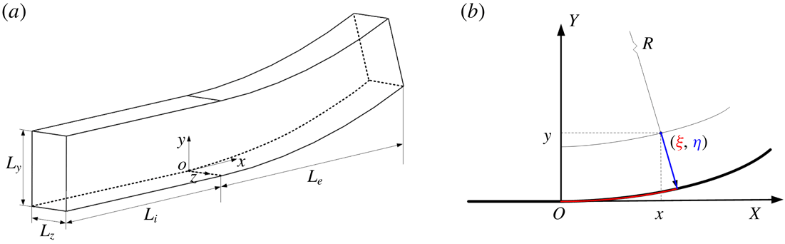In this study, we consider two concave radii of curvature, 908 and 308 mm, and we take $L_{e}=16\unicode[STIX]{x1D6FF}_{0}\approx 100$  mm and the total length of the computational domain is $L_{x}=185$  mm. For brevity, the two concave cases are denoted as CurvR908mm and CurvR308mm for radii of curvature of 908 and 308 mm, respectively. A sketch of the computational domain is shown in figure 1. A fixed coordinate system ( $x,y,z$ ) is used, denoting the streamwise, bottom wall-normal and spanwise directions, respectively, for the straight wall segment. The origin is set at the turning point, which is 85 mm downstream of the inlet. Thus the inlet plane is located at $x=-85$  mm. The curvilinear coordinates $(\unicode[STIX]{x1D709},\unicode[STIX]{x1D702},\unicode[STIX]{x1D701})$ in the concave region are transformed from the Cartesian coordinate system $(x,y,z)$ with $\unicode[STIX]{x1D709}=R\arctan (x/R-y)$ , $\unicode[STIX]{x1D702}=R-r=R-\sqrt{(R-y)^{2}+x^{2}}$ and $\unicode[STIX]{x1D701}=z$ . Thus the coordinate transformation coefficients ( $r_{\unicode[STIX]{x1D709}}$ , $r_{\unicode[STIX]{x1D702}}$ and $r_{\unicode[STIX]{x1D701}}$ ) are known for all cases.

Figure 1.

Sketch of the domain used for the simulations. (a) Sketch of the flat and concave domain. (b) Sketch of the concave radii of curvature.

Table 2.

Grid numbers and stretching control parameters for different cases.

A stretched grid is used near the wall in the $y$ direction, changing gradually to a uniform grid outside the boundary layer with a prescribed spacing. Grid smoothness is very important, especially when high-order schemes are used. Two grid stretching functions with at least second-order continuity at the interface are combined to give coordinates $y_{i}$ in the direction normal to the bottom wall as

(2.8) $$\begin{eqnarray}y_{i}=\left\{\begin{array}{@{}ll@{}}y_{b}{\displaystyle \frac{\sinh (\unicode[STIX]{x1D6FD}\unicode[STIX]{x1D702}_{j})}{\sinh (\unicode[STIX]{x1D6FD})}},\quad \unicode[STIX]{x1D702}_{j}={\displaystyle \frac{j-1}{N_{b}-1}},\quad & j\leqslant N_{b},\\ aj^{5}+bj^{3}+cj+y_{mid},\quad & j>N_{b},\end{array}\right.\end{eqnarray}$$

where $y_{mid}$ is the middle of the domain, while the parameters $a$ , $b$ and $c$ are fixed by continuity considerations up to second order. A predefined distance from the wall, $y_{b}$ , is used to specify the region for grid stretching, with $N_{b}$ the number of grid points inside this region. A fifth-order polynomial enables the grid to change quickly from a stretched grid near the wall to an almost uniform grid away from the wall.

In the $y$ direction, the grid spacing is $y_{1}^{+}=0.8$ for the first point off the wall and $\unicode[STIX]{x0394}y_{\max }^{+}=9.8$ in the centre of the domain (all wall units are calculated based on the inflow friction velocity). The streamwise direction has a uniform grid distribution, with $\unicode[STIX]{x0394}x^{+}=6.5$ . In the spanwise direction, the grid spacing is also uniform and fixed at $\unicode[STIX]{x0394}z^{+}=4.1$ . The grid suitability for the present simulations was also verified by changing the grid resolution in all directions. A sensitive feature was found to be the peak skin friction in the vicinity of the outlet on concave surface which varied by less than $5.0\,\%$ , for a grid that was coarsened by $50\,\%$ in all directions. A variant of the standard total variation diminishing scheme is employed for strong discontinuity capturing (Yee, Sandham & Djomehri Reference Yee, Sandham and Djomehri1999), which is turned off within boundary layers by incorporating the Ducros sensor (Ducros et al. Reference Ducros, Ferrand, Nicoud, Weber, Darracq, Gacherieu and Poinsot1999). Comparisons of mean profiles of flat plate with DNS results of Schlatter & Örlü (Reference Schlatter and Örlü2010) were made and found to be consistent (Sun et al. Reference Sun, Hu and Sandham2017). The boundary-layer thickness at $x=0$  mm is estimated as $\unicode[STIX]{x1D6FF}_{0}\approx 6.19$  mm and the compressible boundary-layer displacement and momentum thicknesses are ${\unicode[STIX]{x1D6FF}_{0}}^{\ast }=2.37$  mm and $\unicode[STIX]{x1D703}_{0}=0.48$  mm, respectively.

No-slip boundary conditions were enforced on the bottom wall (shown in figure 1). The wall temperature is fixed at a value equal to the stagnation temperature of the inflow. Integrated characteristic boundary conditions (Thompson Reference Thompson1990) are used at the outflow and the top boundary. Periodic boundary conditions are applied in the spanwise direction.

Figure 2.

Two-point correlations and energy spectra of the velocity components at different wall-normal locations $x/\unicode[STIX]{x1D6FF}_{0}=11.5$ . (a) Two-point correlations at $y/\unicode[STIX]{x1D6FF}_{0}=0.0587$ . (b) Two-point correlations at $y/\unicode[STIX]{x1D6FF}_{0}=0.2908$ . (c) Energy spectra at $y/\unicode[STIX]{x1D6FF}_{0}=0.0587$ . (d) Energy spectra at $y/\unicode[STIX]{x1D6FF}_{0}=0.2908$ .

2.3 Grid and numerical validity

Statistical data are based on averaging flow fields over 360 non-dimensional time units $(\unicode[STIX]{x1D6FF}_{0}/U_{\infty })$ after running the simulations for 240 non-dimensional units to let the flow develop. To check the spanwise domain size, two-point spanwise correlations of velocity perturbations at different wall-normal locations are given in figure 2(a,b). The correlation definition is the same as in Pirozzoli, Grasso & Gatski (Reference Pirozzoli, Grasso and Gatski2004). As shown, the correlation coefficients decay rapidly to zero with an increase in the spanwise separation. It is clear that the correlation coefficients reduce to zero well within the domain, suggesting that the simulation domain is sufficiently wide to resolve the turbulence dynamics. The adequacy of the spatial resolution is also confirmed by examining the one-dimensional energy spectra (Pirozzoli et al. Reference Pirozzoli, Grasso and Gatski2004), as shown in figure 2(c,d), where $Eu_{a}u_{a}$ is the energy spectrum for the velocity component. It can be seen that all spectra exhibit a drop off of at least four orders of magnitude. Compared to the DNS result of similar flows (Guarini et al. Reference Guarini, Moser, Shariff and Wray2000), these spectra suggest the resolution is adequate.

Turbulent boundary-layer mean velocity profiles and distributions of RMS values at $x=0$  mm on the flat plate (at the concave turning point) are evaluated. The mean inflow profile is generated using the same approach as that of Touber & Sandham (Reference Touber and Sandham2009). The inflow RMS values are taken from the DNS results of Schlatter & Örlü (Reference Schlatter and Örlü2010) for a similar Reynolds number. A compressible scaling, as suggested by Morkovin (Reference Morkovin and Favre1962) and validated by Duan & Beekman (Reference Duan and Beekman2011) for high Mach numbers, is used to transform the incompressible RMS values. The calculated compressible boundary-layer displacement and momentum thicknesses at $x=0$  mm are ${\unicode[STIX]{x1D6FF}_{0}}^{\ast }=2.37$  mm and $\unicode[STIX]{x1D703}_{0}=0.48$  mm, respectively. It should be noted that the Reynolds number based on the free-stream flow properties and the momentum thickness, i.e.  $Re_{\unicode[STIX]{x1D703}}=\unicode[STIX]{x1D70C}_{e}U_{e}\unicode[STIX]{x1D703}/\unicode[STIX]{x1D707}_{w}$ , is 4215. The corresponding Reynolds number under the van Driest scaling, i.e.  $Re_{\unicode[STIX]{x1D703},vd}=\unicode[STIX]{x1D70C}_{w}U_{e}^{vd}\unicode[STIX]{x1D703}^{vd}/\unicode[STIX]{x1D707}_{w}$ , is 1078. 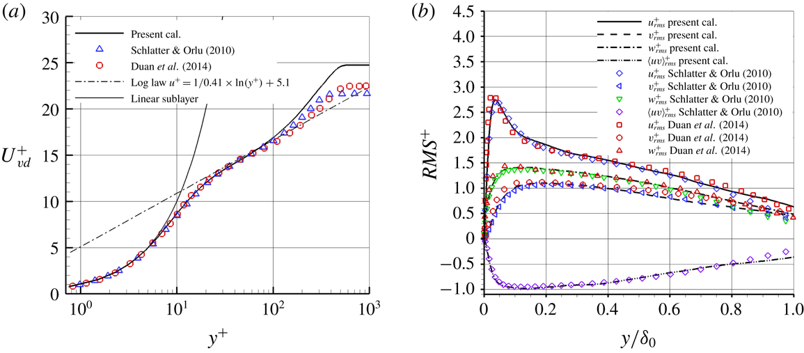The subscripts $e$ and $w$ denote the main flow and wall parameters, respectively, while the superscript $vd$ represents the value under the van Driest transform. Figure 3 shows that the mean and RMS values agree very well with the DNS results of Schlatter & Örlü (Reference Schlatter and Örlü2010), as found in a recent study on turbulent flow over an expansion corner (Sun et al. Reference Sun, Hu and Sandham2017). DNS data of a supersonic boundary layer from Duan & Beekman (Reference Duan and Beekman2011) are also compared in figure 3 and it is found that the current calculation agrees well with the compressible velocity profile and the Reynolds-stress data.

Figure 3.

(a) Mean and (b) RMS velocity distributions obtained at $x=0$  mm on the flat plate, compared with the incompressible flow data of Schlatter & Örlü (Reference Schlatter and Örlü2010) and supersonic flow data of Duan & Beekman (Reference Duan and Beekman2011). The van Driest transformation was applied to the mean velocity and a Morkovin scaling $\unicode[STIX]{x1D709}=\sqrt{\unicode[STIX]{x1D70C}/\unicode[STIX]{x1D70C}_{w}}$ to the RMS curves.

3.1 Mean flow field

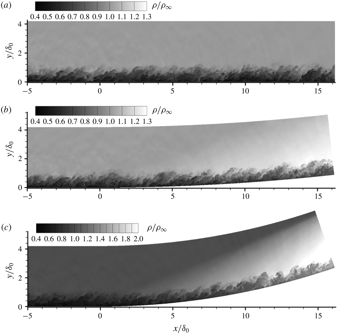
The time-averaged density fields together with sonic lines are given in figure 4 for the whole domain on the left-hand side and in an enlarged view on the right-hand side. It can be seen that the density on the concave surface increases in the main stream and in the boundary layer downstream of the turning point and the compression waves become more evident as the curvature radius decreases. The results correspond to the analysis of Spina et al. (Reference Spina, Smits and Robinson1994), which indicates that the boundary layer on concave walls becomes thinner. The local sonic line is superposed on the contours. Near the outlet, the sonic lines are smooth, with no sign of any artificial disturbances generated near the outflow boundary. An interesting part is that the subsonic region increases as the curvature radius decreases.

Figure 4.

Contours of time-averaged density of the flat plate and the concave cases, normalized by the inflow free-stream density. The local sonic line is superposed on the contour. (a) Flat plate. (b) CurvR908mm. (c) CurvR308mm.

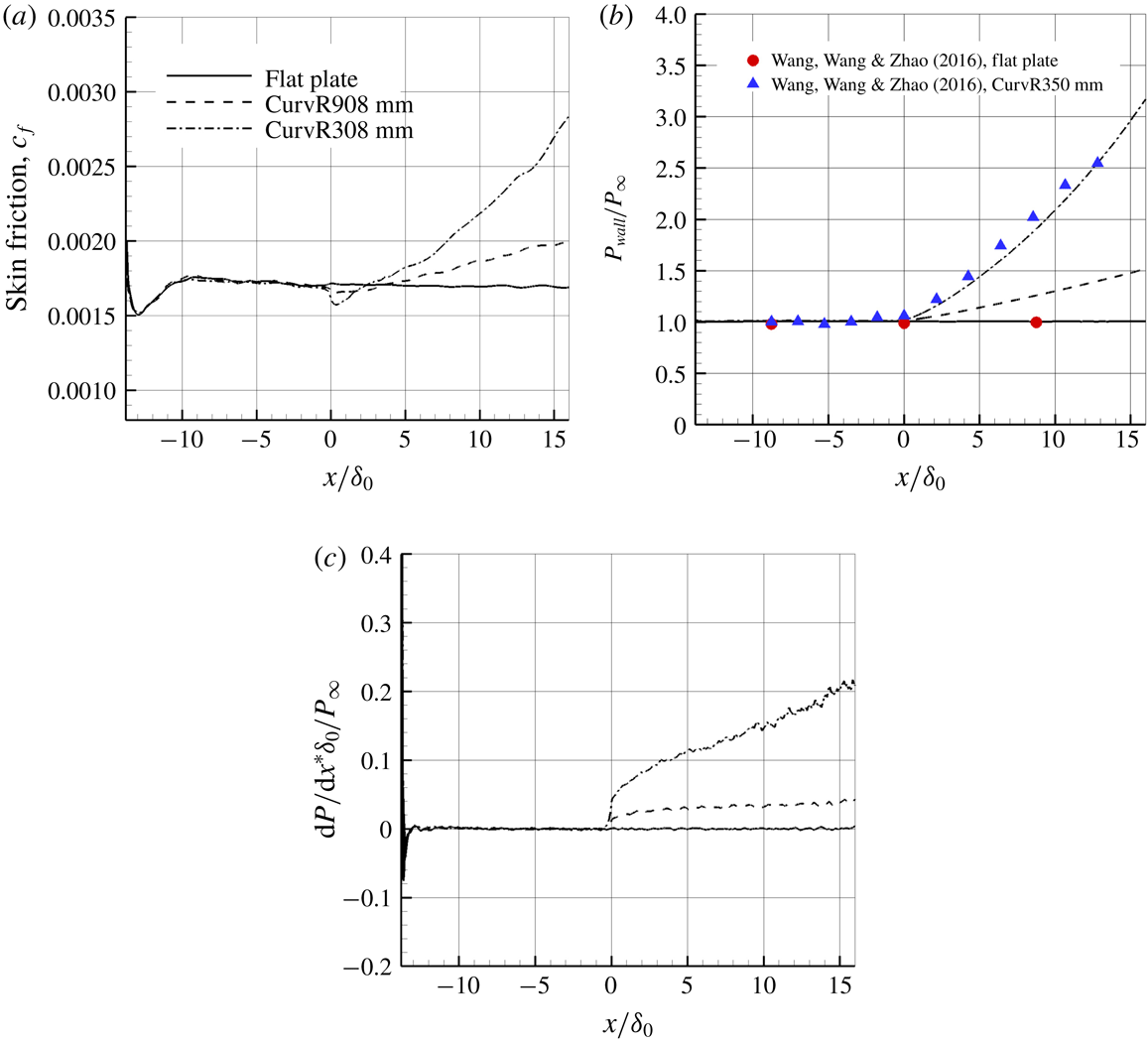
Profiles of the time-averaged skin friction, $C_{f}=2\unicode[STIX]{x1D70F}_{w}/(\unicode[STIX]{x1D70C}_{\infty }U_{\infty }^{2})$ , along the wall for the flat plate and the two concave cases are shown in figure 5. The skin friction starts to follow the expected results (Sun et al. Reference Sun, Hu and Sandham2017) of a turbulent boundary layer by $x/\unicode[STIX]{x1D6FF}_{0}=-5$ , which indicates that the artificial inflow condition recovers to turbulent boundary-layer flow roughly five inflow boundary-layer thicknesses before the turning point $x/\unicode[STIX]{x1D6FF}_{0}=0$ . The skin friction coefficient decreases slightly in the vicinity of the turning point, and increases further downstream, while the pressure increases consistently downstream of the turning point. Experimental data for the wall pressure distribution in a Mach 2.95 supersonic boundary layer (Wang, Wang & Zhao Reference Wang, Wang and Zhao2016b ) are superposed, showing a reasonable agreement. The deviation cannot be discussed further since the uncertainty is not known from the experiments. Figure 5(c) shows the pressure gradient distribution along the wall surface, where it is seen that the pressure gradient has an abrupt increase at $x/\unicode[STIX]{x1D6FF}_{0}=0.0$ for the concave cases and an approximately linear increase for $x/\unicode[STIX]{x1D6FF}_{0}>3$ . The flow on concave walls experiences a continuously increasing pressure all the way to the outflow.

Figure 5.

Mean flow parameters along the flat and concave surfaces. (a) Skin friction coefficient. (b) Wall pressure normalized by the free-stream pressure. (c) Non-dimensional wall pressure gradient.

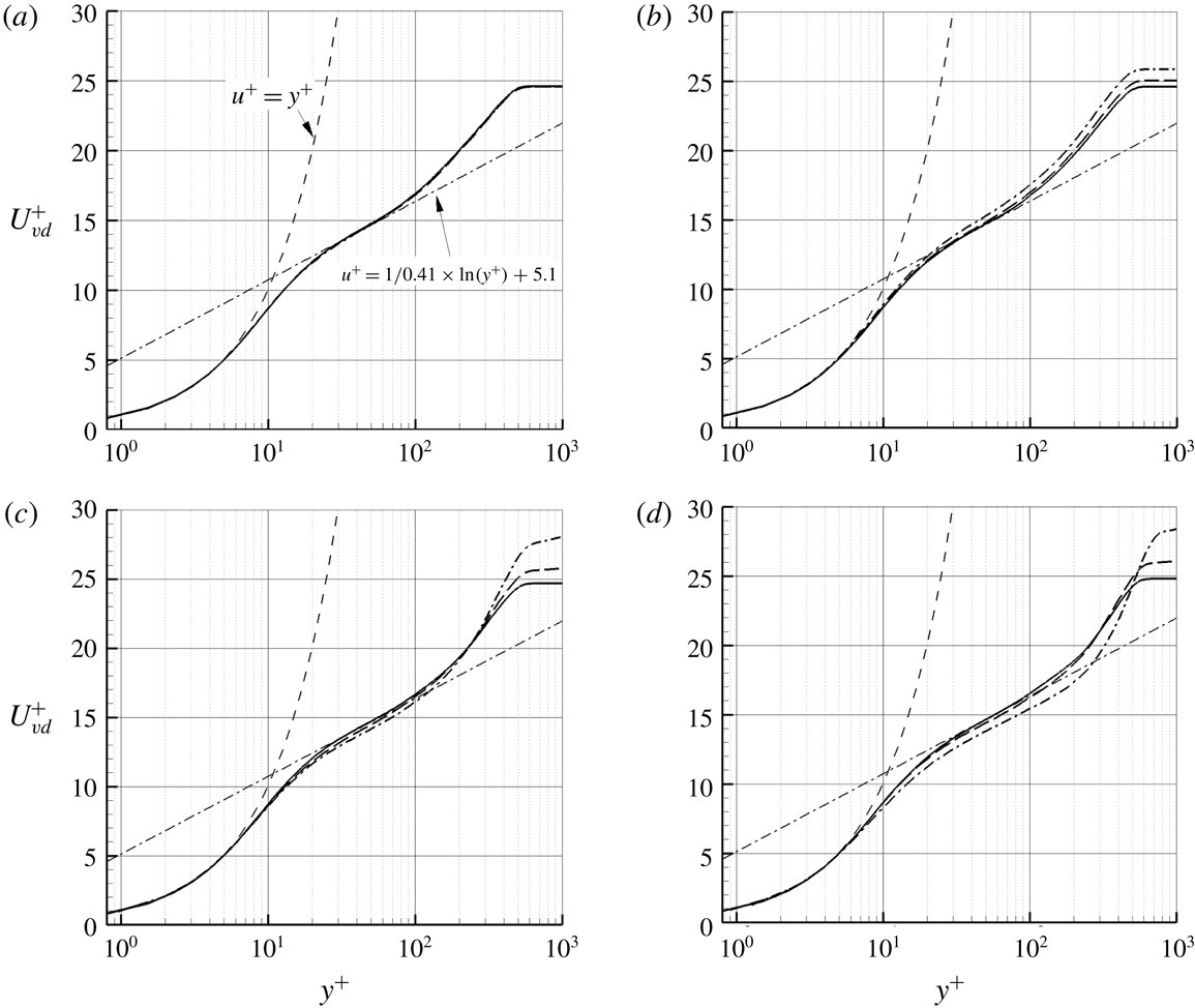
Figure 6 shows velocity profiles both upstream and downstream of the turning point. It can be seen that for concave cases, the velocity on the concave surface is lower than that on the flat plate over most of the boundary layer. Thus, the downstream velocity profiles become less full as the curvature radius increases. In figure 7, the velocity profiles are re-plotted again in wall coordinates using the van Driest transformation, which takes into account the variation of density in compressible boundary layers. Compared to the velocity profiles of the flat plate case, the velocity profiles on concave surfaces deviate slightly from the log-law around the turning point, and the difference becomes more significant further downstream. In the region near the boundary layer outer edge, the wake layer of the CurvR308mm case deviates significantly from the flat plate case.

Figure 6.

Mean velocity profile predictions at different locations (a)  $x/\unicode[STIX]{x1D6FF}_{0}=-2.42$ , (b)  $x/\unicode[STIX]{x1D6FF}_{0}=0.81$ , (c)  $x/\unicode[STIX]{x1D6FF}_{0}=5.65$ and (d)  $x/\unicode[STIX]{x1D6FF}_{0}=10.50$ , normalized by inflow free-stream velocity.

Figure 7.

Mean velocity profile predictions at different locations, with van Driest transformation applied to the mean velocity: (a)  $x/\unicode[STIX]{x1D6FF}_{0}=-2.42$ , (b)  $x/\unicode[STIX]{x1D6FF}_{0}=0.81$ , (c)  $x/\unicode[STIX]{x1D6FF}_{0}=5.65$ and (d)  $x/\unicode[STIX]{x1D6FF}_{0}=10.50$ .

The velocity changes differently in the inner part of the boundary layer of concave cases compared to the flat plate case, as shown in figure 8, where the same velocity profiles as given in figure 7(d) are re-plotted using the outer length scale $\unicode[STIX]{x1D6FF}_{0}$ . Under this scaling, the velocity near the wall increases, which is opposite to the behaviour in the outer region.

Figure 8.

Distribution of velocity as a function of wall-normal distance at $x/\unicode[STIX]{x1D6FF}_{0}=10.50$ normalized by inflow free-stream velocity $U_{\infty }$ (a) and local free-stream velocity $U_{e}$ over the boundary layer (b).

From the turbulent boundary-layer velocity profiles, it is possible to analyse the boundary-layer displacement thickness $\unicode[STIX]{x1D6FF}^{\ast }$ and the momentum thickness $\unicode[STIX]{x1D703}$ , which are defined as $\unicode[STIX]{x1D6FF}^{\ast }=\int _{0}^{h}(1-(\unicode[STIX]{x1D70C}/\unicode[STIX]{x1D70C}_{e})(u/U_{e}))\,\text{d}y$ and $\unicode[STIX]{x1D703}=\int _{0}^{h}(\unicode[STIX]{x1D70C}/\unicode[STIX]{x1D70C}_{e})(u/U_{e})(1-(u/U_{e}))\,\text{d}y$ , respectively. Here we integrate up to $h=1.5\unicode[STIX]{x1D6FF}_{0}$ to reduce the effects of variation in the free-stream properties $\unicode[STIX]{x1D70C}_{e}$ and $U_{e}$ . 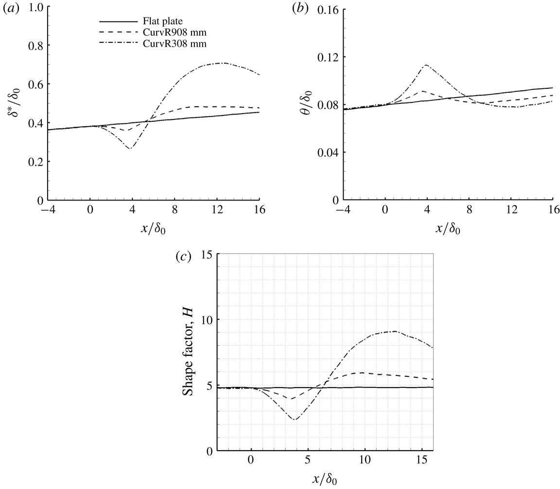Figure 9(a,b) shows the calculated results for different cases. Over the flat plate, both the displacement thickness and momentum thickness grow. Over the concave surfaces, $\unicode[STIX]{x1D6FF}^{\ast }$ experiences a drop after the turning point, followed by a rise downstream of $x/\unicode[STIX]{x1D6FF}_{0}\approx 4.0$ and eventually a reduction. The changes in the higher curvature case are more significant. The momentum thickness $\unicode[STIX]{x1D703}$ first rises above the flat plate values after the turning point, then starts to decrease at $x/\unicode[STIX]{x1D6FF}_{0}\approx 4.0$ , with both curved wall cases eventually having lower values than the flat plate case.

Figure 9.

The displacement thickness $\unicode[STIX]{x1D6FF}^{\ast }$ (a), the momentum thickness $\unicode[STIX]{x1D703}$ (b) and the shape factor $H$ (c) as a function of the streamwise location for the flat and concave cases.

Figure 9(c) shows the shape factor $(H=\unicode[STIX]{x1D6FF}^{\ast }/\unicode[STIX]{x1D703})$ as a function of the streamwise location of both concave cases. As discussed in previous work (Sun et al. Reference Sun, Hu and Sandham2017), a higher shape factor represents a velocity profile with less fullness. It is clearly seen that the shape factor increases significantly further downstream of the turning point on the concave surfaces and then reduces. It is found that $H=8.07$ for the CurvR308mm case at $x/\unicode[STIX]{x1D6FF}_{0}=15.5$ and $H=5.47$ for the CurvR908mm case, compared to $H=4.83$ for the flat plate case.

Figure 10.

The WPSD of pressure on the flat plate and concave walls, normalized by square of free-stream dynamic pressure: (a)  $x/\unicode[STIX]{x1D6FF}_{0}=-2.42$ , (b)  $x/\unicode[STIX]{x1D6FF}_{0}=0.81$ , (c)  $x/\unicode[STIX]{x1D6FF}_{0}=5.65$ and (d)  $x/\unicode[STIX]{x1D6FF}_{0}=10.5$ .

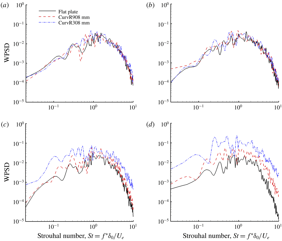
Pressure fluctuations were recorded on the wall surface at different positions for 360 non-dimensional time units with 240 samples. The response of the flow to the curvature is examined by comparing the frequency weighted power spectral density (WPSD), which was calculated using a 50 % segmental averaging method as in Hu, Morfey & Sandham (Reference Hu, Morfey and Sandham2006). As the flow is homogeneous in the spanwise direction, the WPSDs are averaged over the span. The WPSDs given in figure 10 show the pressure fluctuations at various locations for different cases. At $x/\unicode[STIX]{x1D6FF}_{0}=-2.42$ and 0.81, the pressure fluctuations are almost unchanged compared to the flat plate case. At $x/\unicode[STIX]{x1D6FF}_{0}=5.65$ , low-frequency peaks in the spectra appear for concave cases, while at $x/\unicode[STIX]{x1D6FF}_{0}=10.50$ the amplitudes are significantly higher throughout the energy-containing range. Thus the magnitude of the turbulent fluctuations increases with the curvature ratio and, in particular, low-frequency (presumed to be of large scale) structures appear to be generated on concave walls.

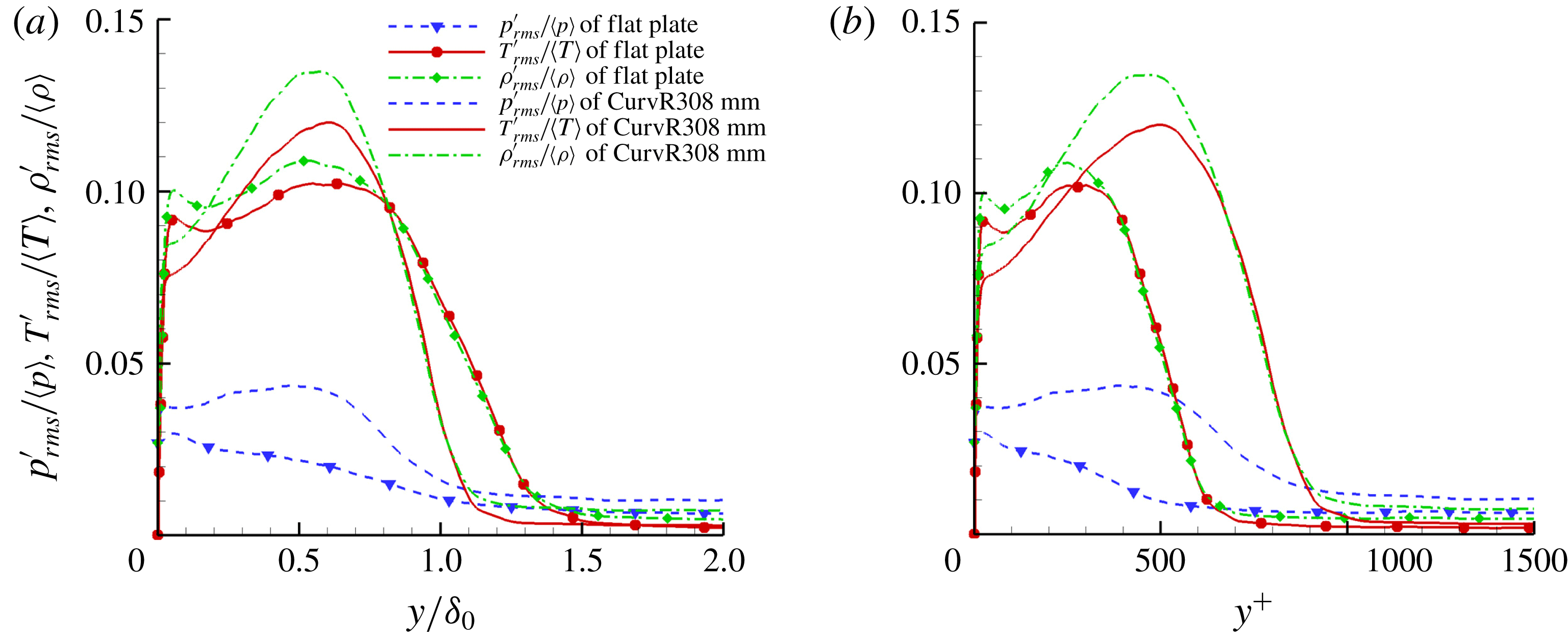
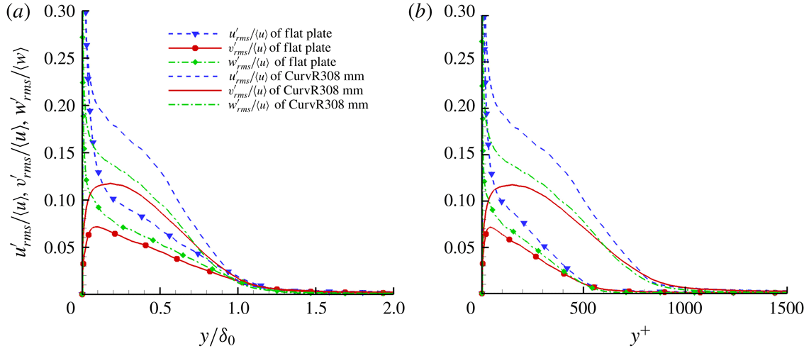
Figure 11 plots RMS values of pressure, temperature and density fluctuation normalized by local averaged $\langle p\rangle$ , $\langle T\rangle$ and $\langle \unicode[STIX]{x1D70C}\rangle$ . It is seen that the local magnitude of density fluctuations on the concave wall is always larger than that on the flat plate. For pressure and temperature fluctuations, the magnitude of the fluctuations increases most obviously in the outer region in the CurvR308mm boundary layer compared to the flat plate. In the inner layer, RMS values of pressure and temperature fluctuations of the CurvR308mm case are lower than those of the flat plate. Figure 12 shows plots of RMS values of velocity fluctuation. It is seen that for velocity fluctuations, the three components of the velocity fluctuations are all increased. These quantitative results exhibit the turbulence amplification from different aspects. The velocity and density fluctuations increase over the entire boundary layer but in the inner layer the pressure and temperature fluctuations are not enhanced, which might be related to the obvious augmentation of the averaged pressure and temperature due to concave compression. Recalling figure 2, the comparison of one-dimensional power spectra between the flat plate case and the concave case at $x/\unicode[STIX]{x1D6FF}_{0}=11.5$ shows that $E_{u_{\unicode[STIX]{x1D6FC}}u_{\unicode[STIX]{x1D6FC}}}$ of CurvR308mm at $y/\unicode[STIX]{x1D6FF}_{0}=0.0587$ is larger in the high-wavenumber region compared to the flat plate. At low wavenumbers, $E_{u_{\unicode[STIX]{x1D6FC}}u_{\unicode[STIX]{x1D6FC}}}$ of the CurvR308mm case is comparable to that of the flat plate, which means that the large-scale turbulence is not obviously enhanced in the inner region of the CurvR308mm boundary layer. At $y/\unicode[STIX]{x1D6FF}_{0}=0.2908$ , $E_{u_{\unicode[STIX]{x1D6FC}}u_{\unicode[STIX]{x1D6FC}}}$ of CurvR308mm is larger than that of the flat plate over the whole wavenumber range. This means that both the small and large scales of turbulence are enhanced.

Figure 11.

Plots of ${p^{\prime }}_{rms}/\langle p\rangle$ , ${\unicode[STIX]{x1D70C}^{\prime }}_{rms}/\langle \unicode[STIX]{x1D70C}\rangle$ and ${T^{\prime }}_{rms}/\langle T\rangle$ versus $y/\unicode[STIX]{x1D6FF}_{0}$ (a) and $y$ unit (b) for different cases at $x/\unicode[STIX]{x1D6FF}_{0}=11.5$ .

Figure 12.

Turbulence intensities of the fluctuating velocity components versus $y/\unicode[STIX]{x1D6FF}_{0}$ (a) and $y$ unit (b) for different cases at $x/\unicode[STIX]{x1D6FF}_{0}=11.5$ .

3.2 Thermal effects

The recovery temperature at the wall $Tr=281.2$  K is calculated according to $T_{r}=T_{\infty }+r(u_{\infty }^{2}/2C_{p})$ , with $r=(\Pr )^{1/3}$ . The recovery temperature has little variation along the curved section. To illustrate the concave wall heat transfer compared to the flat plate, figure 13 gives the Stanton number

(3.1) $$\begin{eqnarray}S_{t}=\frac{q_{w}}{\unicode[STIX]{x1D70C}_{\infty }\unicode[STIX]{x1D70C}_{\infty }C_{p}(T_{w}-T_{r})}\end{eqnarray}$$

along the wall, where $q_{w}=-k(\text{d}\bar{T}/\text{d}y)|_{w}$ .

Figure 13.

Stanton number along the wall in the streamwise direction.

Figure 14.

(a) Mean temperature and (b) wall-normal gradient profiles at $x/\unicode[STIX]{x1D6FF}_{0}=10.50$ .

Figure 15.

SRA profiles at (a)  $x/\unicode[STIX]{x1D6FF}_{0}=0.81$ and (b)  $x/\unicode[STIX]{x1D6FF}_{0}=10.50$ .

Figure 16.

Contours of density flow fields of the flat plate and the concave cases at $z/\unicode[STIX]{x1D6FF}_{0}=1.2$ for (a) flat plate, (b) CurvR908mm and (c) CurvR308mm, normalized by the inflow free-stream density.

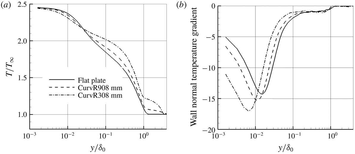
As seen from figure 13, the Stanton number increases on the concave walls compared to the flat plate, and becomes higher as the curvature increases. The temperature profiles depicted in figure 14 show that temperature is higher in the outer region of the concave boundary layer compared to the flat plate. The wall-normal temperature gradient for the concave cases decreases in the outer region but increases in the inner region, leading to the observed increase of the Stanton number on the concave wall. For the CurvR308mm case, the temperature decreases more quickly than for the CurvR908mm case and the flat plate. This tendency is similar to the velocity profile along the wall (analysed in § 3.1), which reflects the different character between the inner layer and the outer layer. The phenomenon is related to the amplification of the turbulence on the concave wall, and will be analysed in the following sections. A test of the strong Reynolds analogy (SRA) is given in figure 15. Morkovin’s SRA is well known for compressible turbulent boundary-layer flows. The SRA is tested using the Morkovin approximate relation (Morkovin Reference Morkovin and Favre1962)

(3.2) $$\begin{eqnarray}\frac{(\overline{T^{\prime \prime 2}})^{1/2}/\tilde{T}}{(\unicode[STIX]{x1D6FE}-1)M_{a}^{2}(\overline{u^{\prime \prime 2}})^{1/2}/\tilde{u} }\approx 1\end{eqnarray}$$

as well as considering the correlation of streamwise velocity and temperature, according to

(3.3) $$\begin{eqnarray}R_{u^{\prime \prime }T^{\prime \prime }}=\frac{-\overline{u^{\prime \prime }T^{\prime \prime }}}{(\overline{u^{\prime \prime 2}})^{1/2}(\overline{T^{\prime \prime 2}})^{1/2}},\end{eqnarray}$$

where a tilde denotes Favre average. Figure 15 shows the results at different streamwise locations. Note that the reference boundary-layer thickness $\unicode[STIX]{x1D6FF}_{0}=6.19$ is measured at the turning point $x/\unicode[STIX]{x1D6FF}_{0}=0.0$ , and the boundary layer on the concave wall is thinner than on the flat plate. That is why figure 15(b) seems slightly different at the edge of the boundary layer. The results show that the SRA relations are satisfied and $R_{u^{\prime \prime }T^{\prime \prime }}$ is almost independent of wall temperature except close to the wall. Through most of the boundary layer, $R_{u^{\prime \prime }T^{\prime \prime }}$ is approximately 0.6, similar to the results reported by Guarini et al. (Reference Guarini, Moser, Shariff and Wray2000), Maeder, Adams & Kleiser (Reference Maeder, Adams and Kleiser1998), Pirozzoli et al. (Reference Pirozzoli, Grasso and Gatski2004) and Duan & Beekman (Reference Duan and Beekman2011). On the concave wall, the SRA relations tend to be satisfied slightly better than along the flat plate.

4.1 Turbulence flow structures

Contours in a two-dimensional slice through instantaneous density fields are given in figure 16. It can be seen that the density on the concave surface increases in the main stream and in the boundary layer downstream of the turning point, and also that compression waves become evident as curvature radius decreases. As measured in previous studies (Donovan et al. Reference Donovan, Spina and Smits1994; Spina et al. Reference Spina, Smits and Robinson1994; Flaherty & Austin Reference Flaherty and Austin2013a ; Wang et al. Reference Wang, Wang and Zhao2016b ), the boundary-layer thickness decreases on a concave wall and on a flat plate with APG in a supersonic flow. In contrast to this, in recent nanoparticle planar laser scattering visualizations of instantaneous two-dimensional flow, Wang & Wang (Reference Wang and Wang2016) observed that the concave boundary layer becomes thicker. From the velocity profiles in the previous section we see that in the present study the boundary layer is on average thinner on concave walls, as seen also in the instantaneous slice shown in figure 16(c). However, another slice at a different spanwise location (figure 17) shows large structures that might be identified as an instantaneous increase of the boundary-layer thickness, which might explain the results of Wang & Wang (Reference Wang and Wang2016). This will be discussed further in § 4.3, and we attribute the variability in thickness to the formation of destabilizing structures with strong instantaneous spanwise variability.

Figure 17.

Contours of density flow fields of the CurvR308mm case at $z/\unicode[STIX]{x1D6FF}_{0}=1.8$ , normalized by the inflow free-stream density.

Figure 18.

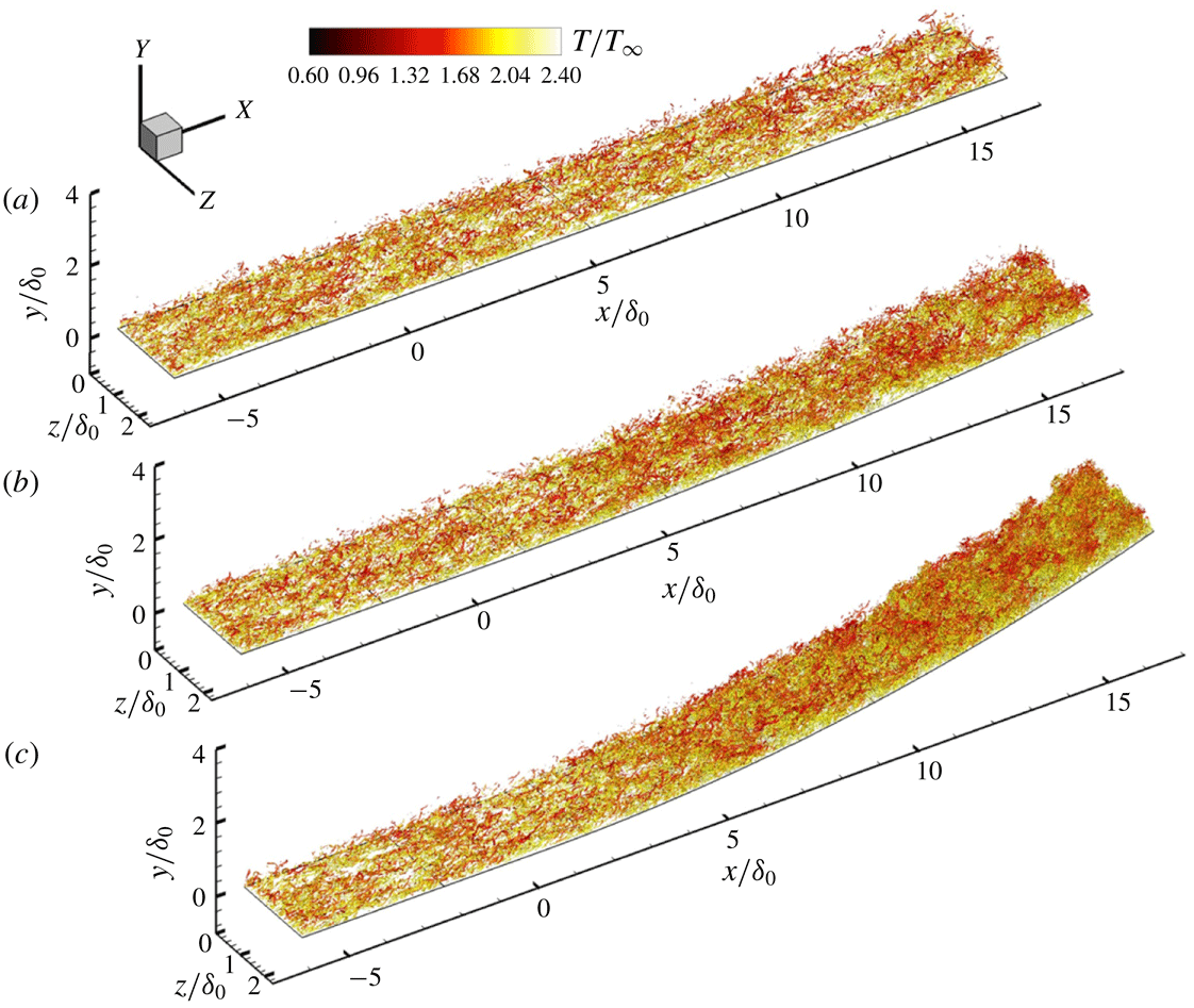
Iso-surface of $\unicode[STIX]{x1D706}_{2}$ coloured by the instantaneous temperature of different cases: (a) flat plate, (b) CurvR908mm and (c) CurvR308mm.

In order to investigate vortex structures before and after the turning point, figure 18 shows an iso-surface of $\unicode[STIX]{x1D706}_{2}$ , which is the second eigenvalue of the $3\times 3$ matrix comprising the velocity gradient components (Jeong & Hussain Reference Jeong and Hussain1995). A small negative value ( $\unicode[STIX]{x1D706}_{2}=-0.3$ ) is selected to visualize the turbulence structures. Compared with the flat plate, supersonic flow past concave surfaces shows an augmentation of $\unicode[STIX]{x1D706}_{2}$ vortices. The turbulence is rapidly amplified in the CurvR308mm case, as shown in figure 18(c). Recalling figures 16(c) and 17, a careful observation of the turbulent structures on the concave wall demonstrates that many smaller fluctuations are superimposed on the large-scale structures. Moreover it is found that new large-scale structures form in the downstream boundary layer on the curved surface.

4.2 Comparison of near-wall streaks and spanwise two-point correlations

The near-wall streaks in the turbulent flow field of the CurvR308mm case are analysed in this section. For the benefit of comparisons between concave cases and the flat plate, the concave wall is plotted in a body-fitted coordinate system $(\unicode[STIX]{x1D709},\unicode[STIX]{x1D702})$ , transforming the computational domain to a rectangular box. The transformed velocity components are given by $u_{t}=u\cos \unicode[STIX]{x1D6FD}-v\sin \unicode[STIX]{x1D6FD}$ and $v_{t}=u\sin \unicode[STIX]{x1D6FD}+v\cos \unicode[STIX]{x1D6FD}$ , respectively, where $\unicode[STIX]{x1D6FD}$ is the local wall turning angle (see figure 1).

The streamwise velocity fields in the transformed coordinates at the same wall-normal distance ( $y/\unicode[STIX]{x1D6FF}_{0}=0.0068$ ) are shown in figure 19(a) from a top view. Alternating low- and high-speed streaks can be clearly identified. The classic near-wall streaks occur in the upstream undisturbed boundary layer in both cases. In the inner layer further downstream, however, the quasi-streamwise structures break down into smaller vortices and an abundance of small structures are generated along the concave wall. The distance between neighbouring low-speed streaks decreases on the concave wall compared to the flat plate case, which will be quantified in the next paragraph with the two-point correlation results. At $y/\unicode[STIX]{x1D6FF}_{0}=0.255$ , shown in figure 19(b), the minimum streamwise velocity of the concave case is lower than that of the flat plate case at the same location, as discussed earlier. Large-scale streaks with enlarged streak spacing are seen on the concave wall, and are found to remain coherent over a long streamwise distance.

Figure 19.

Streamwise velocity contours at (a)  $y/\unicode[STIX]{x1D6FF}_{0}=0.0068$ and (b)  $y/\unicode[STIX]{x1D6FF}_{0}=0.255$ slices of the flat plate (top) and the CurvR308mm (bottom) cases.

To quantify the distance between two neighbouring low-speed streaks, two-point spanwise correlations of velocity perturbations are compared between the flat plate and the CurvR308mm cases at $x/\unicode[STIX]{x1D6FF}_{0}=15.5$ for different wall-normal distance, as given in figure 20. At $y/\unicode[STIX]{x1D6FF}_{0}=0.0068$ (figure 20 a) in the flat plate case, the minimum of the wall-normal velocity correlation is found at $z/\unicode[STIX]{x1D6FF}_{0}=0.045$ , which is the typical streak spacing in a zero-pressure-gradient boundary layer. For the CurvR308mm case, the streak width is significantly reduced, consistent with the increasing skin friction. This is in contrast to the behaviour away from the wall, where at $y/\unicode[STIX]{x1D6FF}_{0}=0.255$ (figure 19), an increase in the streak spacing compared to the flat plate case can be identified. This indicates that streaks might be organized into new patterns, corresponding to the large-velocity streaks seen in figure 19.

Figure 20.

Two-point spanwise correlations for velocity perturbations at $x/\unicode[STIX]{x1D6FF}_{0}=15.5$ : (a)  $y/\unicode[STIX]{x1D6FF}_{0}=0.0068$ and (b)  $y/\unicode[STIX]{x1D6FF}_{0}=0.255$ . The spanwise coordinates are normalized by the boundary-layer thickness $\unicode[STIX]{x1D6FF}_{0}$ .

4.3 Iso-surfaces and slices of instantaneous velocity in three-dimensional flow field

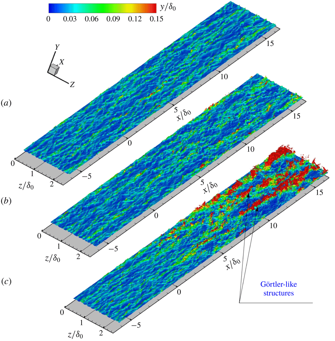
To understand the changes in coherent structures, iso-surfaces of the streamwise velocity, together with streamlines coloured by the wall-normal distance are illustrated and compared in figures 21 and 22. All the results are based on the domain transformation introduced in § 4.2.

Figure 21.

Turbulence coherent structures visualized with the iso-surface of $u_{t}/U_{\infty }=0.4$ coloured by the wall-normal distance. (a) Flat plate. (b) CurvR908mm. (c) CurvR308mm.

Figure 22.

Oblique view of three-dimensional streamlines originating from inflow wall parallel plane $y/\unicode[STIX]{x1D6FF}_{0}=0.0266$ and $x/\unicode[STIX]{x1D6FF}_{0}=-6.0$ , coloured by the wall-normal distance in $y/\unicode[STIX]{x1D6FF}_{0}$ unit. (a) Flat plate. (b) CurvR908mm. (c) CurvR308mm.

From figure 21, it is clear that smaller concave curvature radius (CurvR308mm), which means higher curvature ratio, tends to destabilize structures in the boundary layer. For the flat plate case shown in figure 21(a), we can clearly see the classic elongated streamwise structures in the iso-surface of $u_{t}=0.4$ . For the CurvR908mm case, the streaks are preserved, but the streaks appear more corrugated and lifted away from the concave wall. Upstream and for a short distance downstream ( $x/\unicode[STIX]{x1D6FF}_{0}<5$ ) of the turning point, the structures are very similar to those of the flat plate case. However, further downstream the structures start to produce smaller streaks. Most of the structures remain close to the wall as in the flat plate case. For the CurvR308mm case, the streaks on the concave wall develop into a new pattern and large-scale organized structures are lifted away from the wall into the outer layer. The orientation of these structures suggests that they are likely to be the Görtler-like structures previously shown in numerical simulations of hypersonic flow (Ren & Fu Reference Ren and Fu2015a ). From a comparison of figure 21(a–c), we can see that the concave effects strengthen the lift-up process of velocity streaks in the boundary layer, with the Görtler-like vortices pumping fluid packets from the inner layer outwards. Recalling the pressure fluctuation discussed in § 3.2, since Görtler instabilities lead to coherent large-scale structures in the concave boundary layer, the reason for the low-frequency pressure fluctuations becomes apparent. Observation on the iso-surface of $u_{t}=0.4$ at different time points reveals that the Görtler-like structures drift in the spanwise direction as time changes. Since they are not fixed in space, these structures cannot be investigated from an averaged view.

Figure 22 shows representative instantaneous streamlines, originating in the $y/\unicode[STIX]{x1D6FF}_{0}=0.0266$ plane and $x/\unicode[STIX]{x1D6FF}_{0}=-6.0$ upstream of the turning point. These streamlines, coloured by the wall-normal distance, illustrate the motion of the fluid. It is seen that the initially planar streamlines are lifted and tilted downstream of the turning point. For the flat plate case, the streamlines concentrate into streaky structures and are convected downstream. For the concave cases, the streamlines form into lifted streaks, consistent with the generation of Görtler-like vortices, and illustrate how the streamlines transport fluid from the upstream inner boundary layer to the outer layer downstream.

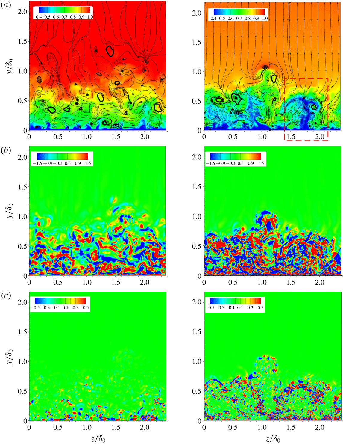
Figure 23(a) shows contours of the local velocity contour superimposed with the local in-plane streamlines for the instantaneous flow at $x/\unicode[STIX]{x1D6FF}_{0}=11.5$ . The predominant wall-normal flow on concave surface outside the boundary layer is due to surface curvature centrifugal effect. The region shown in the dashed-line window is an example of a mushroom structure, which is likely to be the typical consequence of a Görtler vortex, as in concave laminar flow (Ren & Fu Reference Ren and Fu2015a ). It is seen that the low-momentum fluid in the inner boundary layer is pumped into the outer layer by the Görtler-like structures. Figure 23(b) shows that small-scale vortices are more abundant on the concave wall. Combined with the $\unicode[STIX]{x1D706}_{2}$ vortex structures in figure 18(c) and the streaks in the inner boundary layer in figure 19, we can tell that small-scale turbulence is enhanced in the concave boundary layer. The vorticity transport equation can be written as

(4.1) $$\begin{eqnarray}\frac{\text{D}\unicode[STIX]{x1D74E}}{\text{D}t}=(\unicode[STIX]{x1D74E}\boldsymbol{\cdot }\unicode[STIX]{x1D735})\boldsymbol{u}-\unicode[STIX]{x1D74E}(\unicode[STIX]{x1D735}\boldsymbol{\cdot }\boldsymbol{u})-\frac{\unicode[STIX]{x1D735}p\times \unicode[STIX]{x1D735}\unicode[STIX]{x1D70C}}{\unicode[STIX]{x1D70C}^{2}}+\unicode[STIX]{x1D735}\times \left(\frac{\unicode[STIX]{x1D735}\boldsymbol{\cdot }\unicode[STIX]{x1D70F}}{\unicode[STIX]{x1D70C}}\right).\end{eqnarray}$$

The third term, $\unicode[STIX]{x1D735}p\times \unicode[STIX]{x1D735}\unicode[STIX]{x1D70C}/\unicode[STIX]{x1D70C}^{2}$ , describes vorticity production via the baroclinic mechanism, which occurs when the density and pressure gradients are misaligned. Pressure enters the vorticity equation only through this baroclinic term. It is important to note that vorticity can be generated by baroclinic torque in the concave flow, whereas the other terms in the vorticity equation describe the amplification, stretching, bending or diffusion of existing vorticity. The baroclinic production term is given by

(4.2) $$\begin{eqnarray}\displaystyle \boldsymbol{B}_{p} & = & \displaystyle \frac{(\unicode[STIX]{x1D735}p\times \unicode[STIX]{x1D735}\unicode[STIX]{x1D70C})}{\unicode[STIX]{x1D70C}^{2}}=\frac{1}{\unicode[STIX]{x1D70C}^{2}}\left(\frac{\unicode[STIX]{x2202}\unicode[STIX]{x1D70C}}{\unicode[STIX]{x2202}y}\frac{\unicode[STIX]{x2202}p}{\unicode[STIX]{x2202}z}-\frac{\unicode[STIX]{x2202}\unicode[STIX]{x1D70C}}{\unicode[STIX]{x2202}z}\frac{\unicode[STIX]{x2202}p}{\unicode[STIX]{x2202}y}\right)\boldsymbol{i}+\frac{1}{\unicode[STIX]{x1D70C}^{2}}\left(\frac{\unicode[STIX]{x2202}\unicode[STIX]{x1D70C}}{\unicode[STIX]{x2202}z}\frac{\unicode[STIX]{x2202}p}{\unicode[STIX]{x2202}x}-\frac{\unicode[STIX]{x2202}\unicode[STIX]{x1D70C}}{\unicode[STIX]{x2202}x}\frac{\unicode[STIX]{x2202}p}{\unicode[STIX]{x2202}z}\right)\boldsymbol{j}\nonumber\\ \displaystyle & & \displaystyle +\,\frac{1}{\unicode[STIX]{x1D70C}^{2}}\left(\frac{\unicode[STIX]{x2202}\unicode[STIX]{x1D70C}}{\unicode[STIX]{x2202}x}\frac{\unicode[STIX]{x2202}p}{\unicode[STIX]{x2202}y}-\frac{\unicode[STIX]{x2202}\unicode[STIX]{x1D70C}}{\unicode[STIX]{x2202}y}\frac{\unicode[STIX]{x2202}p}{\unicode[STIX]{x2202}x}\right)\boldsymbol{k}\end{eqnarray}$$

or

(4.3) $$\begin{eqnarray}\displaystyle \frac{\left(\unicode[STIX]{x1D735}p\times \unicode[STIX]{x1D735}\unicode[STIX]{x1D70C}\right)}{\unicode[STIX]{x1D70C}^{2}} & = & \displaystyle \frac{1}{\unicode[STIX]{x1D70C}^{2}}r_{\unicode[STIX]{x1D702}}r_{\unicode[STIX]{x1D701}}\left(\frac{\unicode[STIX]{x2202}\unicode[STIX]{x1D70C}}{\unicode[STIX]{x2202}\unicode[STIX]{x1D702}}\frac{\unicode[STIX]{x2202}p}{\unicode[STIX]{x2202}\unicode[STIX]{x1D701}}-\frac{\unicode[STIX]{x2202}\unicode[STIX]{x1D70C}}{\unicode[STIX]{x2202}\unicode[STIX]{x1D701}}\frac{\unicode[STIX]{x2202}p}{\unicode[STIX]{x2202}\unicode[STIX]{x1D702}}\right)\boldsymbol{i}\nonumber\\ \displaystyle & & \displaystyle +\,\frac{1}{\unicode[STIX]{x1D70C}^{2}}r_{\unicode[STIX]{x1D709}}r_{\unicode[STIX]{x1D701}}\left(\frac{\unicode[STIX]{x2202}\unicode[STIX]{x1D70C}}{\unicode[STIX]{x2202}\unicode[STIX]{x1D701}}\frac{\unicode[STIX]{x2202}p}{\unicode[STIX]{x2202}\unicode[STIX]{x1D709}}-\frac{\unicode[STIX]{x2202}\unicode[STIX]{x1D70C}}{\unicode[STIX]{x2202}\unicode[STIX]{x1D709}}\frac{\unicode[STIX]{x2202}p}{\unicode[STIX]{x2202}\unicode[STIX]{x1D701}}\right)\boldsymbol{j}+\frac{1}{\unicode[STIX]{x1D70C}^{2}}r_{\unicode[STIX]{x1D709}}r_{\unicode[STIX]{x1D702}}\left(\frac{\unicode[STIX]{x2202}\unicode[STIX]{x1D70C}}{\unicode[STIX]{x2202}\unicode[STIX]{x1D709}}\frac{\unicode[STIX]{x2202}p}{\unicode[STIX]{x2202}\unicode[STIX]{x1D702}}-\frac{\unicode[STIX]{x2202}\unicode[STIX]{x1D70C}}{\unicode[STIX]{x2202}\unicode[STIX]{x1D702}}\frac{\unicode[STIX]{x2202}p}{\unicode[STIX]{x2202}\unicode[STIX]{x1D709}}\right)\boldsymbol{k},\qquad\end{eqnarray}$$

which indicates the rate at which the vorticity is generated.

Figure 23(c) shows the distribution of the baroclinic production term on a slice at $x/\unicode[STIX]{x1D6FF}_{0}=11.5$ . The baroclinic production term in the outer region of the concave boundary layer has a higher magnitude than on the flat plate and arises near the interface of the high-speed flow with the low-speed flow, corresponding to the Görtler-like structures shown in figure 23(a). In (4.2), the normal pressure gradient $\unicode[STIX]{x2202}P/\unicode[STIX]{x2202}y$ (from centrifugal effects) can interact with spanwise density gradient $\unicode[STIX]{x2202}\unicode[STIX]{x1D70C}/\unicode[STIX]{x2202}z$ , leading to streamwise vorticity induced by these interactions. Therefore it is concluded that the Görtler-like vortices occurring in the outer region of the concave boundary layer can easily twist the original density and pressure gradients. Prominent pressure gradients interact with the density gradients and induce significant vorticity in the concave boundary layer. This corresponds to the generation of the abundant small vortices shown in figure 23(b). In the inner region, pressure gradients interact with the local density gradients and cause more vortices than the flat plate with zero pressure gradient while the influence of the Görtler instability on density gradients appears smaller.

Figure 23.

Streamwise velocity, vorticity and baroclinic production contours for the flat plate (left) and the CurvR308mm (right) case at $x/\unicode[STIX]{x1D6FF}_{0}=11.5$ . (a) Streamwise velocity ( $\text{u}_{t}/\text{U}_{\infty }$ ) contours, superimposed with in-plane streamlines. (b) Streamwise vorticity ( $\unicode[STIX]{x1D714}_{x}/(\text{U}_{\infty }/\unicode[STIX]{x1D6FF}_{0})$ ) distribution. (c) Baroclinic production ( $|B_{p}|/(U_{\infty }^{2})/\unicode[STIX]{x1D6FF}_{0}^{2}$ ).

The evolution of turbulent flow structures can be quantified using the anisotropy invariant map (Lumley Reference Lumley1978). This map comprises the second and third invariants of the Reynolds stress anisotropy tensor $(\unicode[STIX]{x1D623}_{ij})$ , which are defined as

(4.4) $$\begin{eqnarray}\left.\begin{array}{@{}c@{}}\displaystyle \unicode[STIX]{x1D623}_{ij}=\frac{\left\langle \unicode[STIX]{x1D70C}u_{i}^{\prime \prime }u_{j}^{\prime \prime }\right\rangle }{\left\langle \unicode[STIX]{x1D70C}u_{k}^{\prime \prime }u_{k}^{\prime \prime }\right\rangle }-\frac{1}{3}\unicode[STIX]{x1D6FF}_{ij},\\ \displaystyle II_{b}=\unicode[STIX]{x1D623}_{ij}\unicode[STIX]{x1D623}_{ji},\\ \displaystyle III_{b}=\unicode[STIX]{x1D623}_{ij}\unicode[STIX]{x1D623}_{jk}\unicode[STIX]{x1D623}_{ki}.\end{array}\right\}\end{eqnarray}$$

Figure 24.

Anisotropy invariant maps based on ( $\text{III}_{b}$ , $\text{II}_{b}$ ) and ( $\unicode[STIX]{x1D6F9},\unicode[STIX]{x1D711}$ ) respectively at $x/\unicode[STIX]{x1D6FF}_{0}=11.5$ for different cases. (a) Overall and (b) enlarged view.

Figure 24(a) shows the anisotropy invariant map at $x/\unicode[STIX]{x1D6FF}_{0}=11.5$ , with an expanded view of the part near the outer edge of the boundary layer in figure 24(b). It can be seen that there are significant changes over the concave surface. The near-wall region still approaches the two-component limit, but does so further from the one-component point, consistent with less well organized near-wall velocity streaks. The maximum anisotropy occurred in the CurvR308mm case at $y/\unicode[STIX]{x1D6FF}_{0}=0.0084$ , which falls approximately in the buffer layer. At the outer edge of the boundary layer the convex wall cases become closer to isotropic and the turbulence state spends more time close to axisymmetric compression. These characteristics are also observed in the DNS conducted by Grilli, Hickel & Adams (Reference Grilli, Hickel and Adams2013) and Tong et al. (Reference Tong, Li, Duan and Yu2017). Based on a comparison with figures 11 and 12, the anisotropy results are in accordance with the two-layer structure of the concave boundary layer.

Figure 25.

Schematic of Görtler instabilities in a supersonic concave boundary layer and the small vortices formed by the large baroclinic production induced by the density gradient from Görtler-like vortices and the pressure gradient from concave compression. (a) Görtler instabilities in the outer portion of the boundary layer twist the local gradient. (b) Baroclinic effects on the boundary layer experiencing an APG. (c) Görtler vortices promote exchange process in the outer boundary layer.

It is difficult to extract Görtler-like vortices from the chaotic background shown in figure 23(a,b), and this is probably the reason why no experiments have found Görtler-like vortices under turbulent conditions. Ren & Fu (Reference Ren and Fu2015b ) used instability analysis to show the nonlinear development of Görtler vortices and the formation of low- and high-speed streaks in a laminar supersonic boundary layer at Mach 3.0. Their results showed that a mushroom structure is developed in the flow field. As mentioned above, there is no regular Görtler structure in the current turbulent flow where small vortices stir and break down the large scales. However, the structures showed up clearly in the streamline plots of figure 22. It is believed that the Görtler vortices feed the generation of large numbers of small vortices and significantly promote the exchange of the inner layer with the outer layer. On the concave wall, the inner region is mainly affected by the APG and the local turbulence amplification can be explained by previous research (Lee & J.Sung Reference Lee and Sung2009; Franko & Lele Reference Franko and Lele2014) on flat plate supersonic boundary layers. As previously noted, the APG interacts with the density gradients formed around streaks in the inner layer, and the resulting baroclinic effects lead to the formation of many small vortices, as seen in figure 19.

Figure 25 summarizes the role of Görtler instabilities in the turbulent supersonic concave boundary layer. A schematic view of the Görtler vortices is shown in figure 25(a), which shows a typical mushroom shape and the associated modulation of the inner boundary layer. The important result is that Görtler vortices twist and distort the local density gradient. Figure 25(b) shows the inner region flow interaction with APG, which also represents the boundary-layer interaction with the APG without centrifugal effects. As given in previous studies (?Donovan et al. Reference Donovan, Spina and Smits1994; Flaherty & Austin Reference Flaherty and Austin2013b ; Wang, Wang & Zhao Reference Wang, Wang and Zhao2016a ), the boundary-layer thickness on the flat plate decreases when subject to APG. Comparing figures 25(a) and 25(b), the prominent difference is that the Görtler vortices induce stretching, twisting and distortion of the density gradient surfaces to intersect with compression wave sheet, which generate a larger baroclinic effect to induce more vortices than on the flat plate. Figure 25(c) shows that the compression waves interact with the Görtler vortices and induce abundant small vortices. It might be argued that incompressible flow on concave walls would also contain Görtler vortices and a turbulence augmentation through vortex breakdown. However, a favourable pressure gradient and a uniform density for incompressible flow on concave walls would slow down the turbulence production and even lead to relaminarization (Fernholz & Warnack Reference Fernholz and Warnack1998). For the supersonic boundary layer, favourable pressure gradients similarly weaken the coherent structures (Spalart & Watmuff Reference Spalart and Watmuff1993; Tichenor et al. Reference Tichenor, Humble and Bowersox2013; Sun et al. Reference Sun, Hu and Sandham2017) and lead to a turbulence suppression in the outer region of the boundary layer. For the supersonic concave boundary layer, as found by Kim, Samimy & Lee (Reference Kim, Samimy and Lee2001), the turbulence amplification was closely related to the linear increase in the mean density during the supersonic compression. It could be inferred that baroclinic effects are important and seem to be fundamental for the formation of small vortices and the corresponding turbulence augmentation. In the next section we will give more quantitative results based on TKE budgets.

5.1 Turbulent kinetic energy distribution

Figure 26.

The RMS velocity distributions at different streamwise locations, normalized by free-stream velocity. Solid black lines represent the CurvR308mm case. Dash-dotted red lines represent the flat plate case. The RMS velocity of the streamwise (●), wall-normal (▾), spanwise (▴) and velocity fluctuations, together with Reynolds shear stress (♦): (a)  $x/\unicode[STIX]{x1D6FF}_{0}=-2.42$ , (b)  $x/\unicode[STIX]{x1D6FF}_{0}=0.81$ , (c)  $x/\unicode[STIX]{x1D6FF}_{0}=5.65$ and (d)  $x/\unicode[STIX]{x1D6FF}_{0}=10.50$ .

Figure 26 compares the RMS values of all three velocity components and the Reynolds stress ( $\langle -u^{\prime }v^{\prime }\rangle$ ) on the flat plate and in the CurvR308mm case at different streamwise locations. On the concave wall, velocity fluctuations for all components are amplified. Just downstream of the turning point, the turbulence level increases slightly. Whereas the inner layer peaks are almost unchanged, in the outer layer turbulence is significantly augmented along the concave wall, and the magnitudes of all velocity fluctuations are larger than those of the flat plate case.

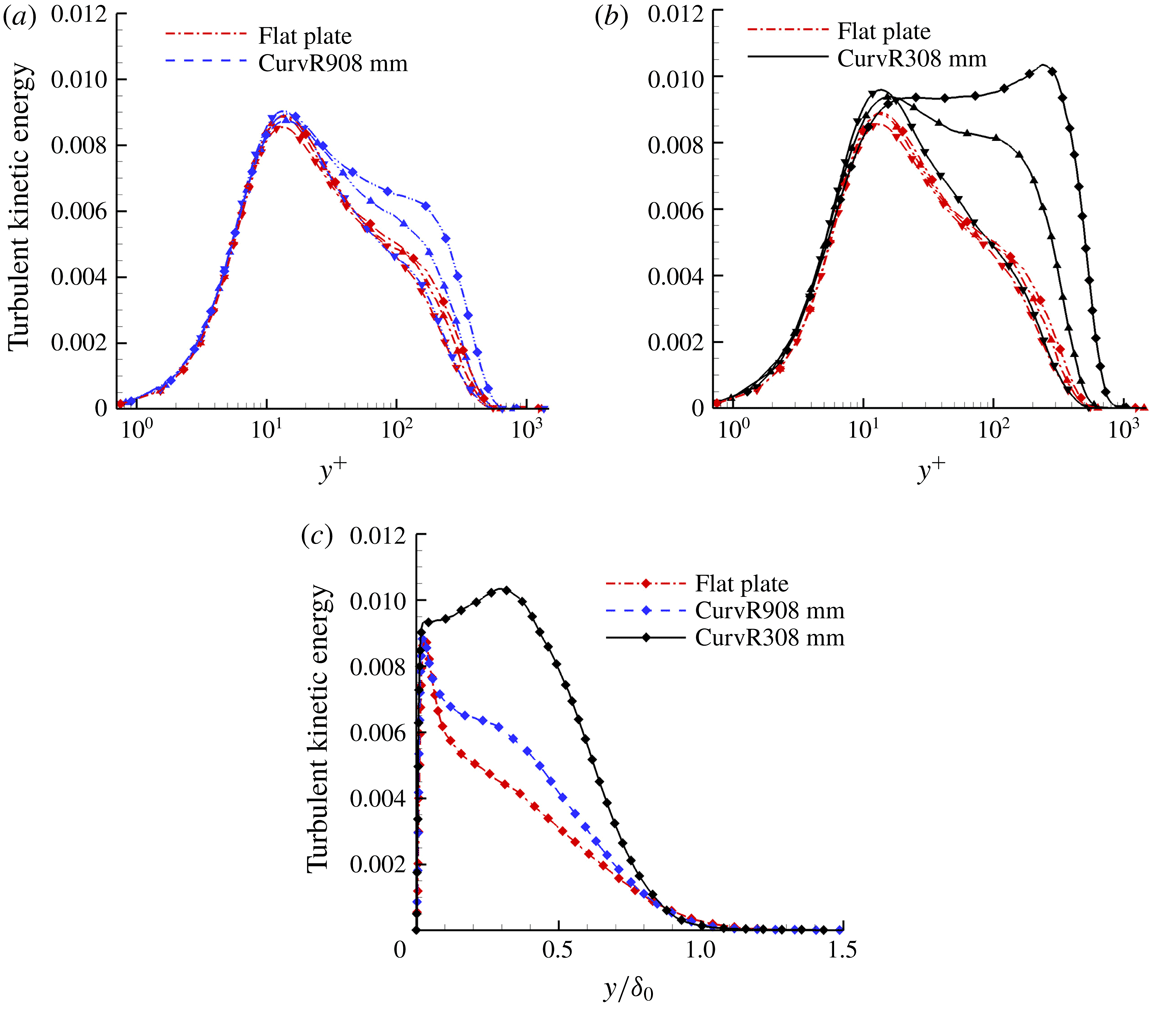
The TKE is defined as $\tilde{k}=\overline{\unicode[STIX]{x1D70C}u_{i}^{\prime \prime }u_{i}^{\prime \prime }}/2\bar{\unicode[STIX]{x1D70C}}$ , where the superscript refers to fluctuations from the Favre averages. The TKE profiles at different streamwise locations of various cases are shown in figure 27. As expected, significant amplification of the TKE occurs on the concave surface. Turbulence in the inner layer of the boundary layer (i.e. the inner peak at $y^{+}=12$ ) increases downstream of the turning point compared to the same location on the flat plate, but then decreases along the concave wall. By contrast, the outer layer of the boundary layer experiences strong turbulence amplification and an outer peak emerges. A smaller curvature radius (CurvR308mm) results in a larger amplification across the boundary layer, shown in figure 27(c). Therefore, a strong two-layer structure of turbulence can be identified in the concave region. The structure is attributed to the turbulence shear stress amplification in the boundary layer on the concave wall, presumed to be due to the large-scale Görtler structures, while the inner boundary layer remains in local equilibrium. The phenomenon of the outer peak formation is similar to the second outer peak occurring in high Reynolds number wall flow. Vallikivi, Ganapathisubramani & Smits (Reference Vallikivi, Ganapathisubramani and Smits2015a ) and Vallikivi, Hultmark & Smits (Reference Vallikivi, Hultmark and Smits2015b ) showed that for low Reynolds numbers there is no TKE peak in the outer layer of zero-pressure-gradient boundary layer, while for very high Reynolds number, a peak emerges in the outer layers. Smits, McKeon & Marusic (Reference Smits, McKeon and Marusic2011) summarized researches on high Reynolds number ( $46\,700\leqslant Re_{\unicode[STIX]{x1D703}}\leqslant 235\,000$ ) wall turbulence and indicated that very-large-scale motions make a significant contribution to the TKE and Reynolds stress production in the logarithmic and outer layer. This is relevant here since Görtler vortices play an important role in turbulence amplification for concave flows, whereas for high Reynolds number wall turbulence, the origin of the very-large-scale motions is still a challenging problem (Smits et al. Reference Smits, McKeon and Marusic2011).

Figure 27.

Turbulence kinetic energy profile comparison of various cases at different streamwise locations. (a) Comparison between flat plate and CurvR908mm case at $x/\unicode[STIX]{x1D6FF}_{0}=0.81$ (▾), $x/\unicode[STIX]{x1D6FF}_{0}=5.65$ (▴) and $x/\unicode[STIX]{x1D6FF}_{0}=10.50$ (♦). (b) Comparison between flat plate and CurvR308mm case at $x/\unicode[STIX]{x1D6FF}_{0}=0.81$ (▾), $x/\unicode[STIX]{x1D6FF}_{0}=5.65$ (▴) and $x/\unicode[STIX]{x1D6FF}_{0}=10.50$ (♦). (c) Comparison between flat plate, CurvR908mm case and CurvR308mm case at $x/\unicode[STIX]{x1D6FF}_{0}=15.35$ (♦). Dash-dotted line represents flat plate case. Dashed line represents CurvR908mm case. Solid line represents CurvR308mm case.

5.2 Turbulent kinetic energy budgets

The evaluation of budgets of the TKE mainly focuses on the following terms. The explicit forms of the different terms are given in Guarini et al. (Reference Guarini, Moser, Shariff and Wray2000) and Sun et al. (Reference Sun, Hu and Sandham2017) and briefly listed below:

(5.1) $$\begin{eqnarray}\frac{\unicode[STIX]{x2202}}{\unicode[STIX]{x2202}t}(\bar{\unicode[STIX]{x1D70C}}\bar{k})+\tilde{u} _{j}\frac{\unicode[STIX]{x2202}}{\unicode[STIX]{x2202}x_{j}}(\bar{\unicode[STIX]{x1D70C}}\bar{k})=P+T+II+D-\unicode[STIX]{x1D719}+V_{c},\end{eqnarray}$$

where

(5.2) $$\begin{eqnarray}\displaystyle & \displaystyle P=-\overline{\unicode[STIX]{x1D70C}u_{i}^{\prime \prime }u_{j}^{\prime \prime }}\frac{\unicode[STIX]{x2202}\tilde{u} _{i}}{\unicode[STIX]{x2202}x_{j}}, & \displaystyle\end{eqnarray}$$

(5.3) $$\begin{eqnarray}\displaystyle & \displaystyle T=-\frac{1}{2}\frac{\unicode[STIX]{x2202}}{\unicode[STIX]{x2202}x_{j}}\overline{\unicode[STIX]{x1D70C}u_{i}^{\prime \prime }u_{i}^{\prime \prime }u_{j}^{\prime \prime }}, & \displaystyle\end{eqnarray}$$

(5.4) $$\begin{eqnarray}\displaystyle & \displaystyle II=II_{t}+II_{d}=-\frac{\unicode[STIX]{x2202}}{\unicode[STIX]{x2202}x_{j}}\overline{p^{\prime }u_{i}^{\prime \prime }}\unicode[STIX]{x1D6FF}_{ij}+\overline{p^{\prime }\frac{\unicode[STIX]{x2202}u_{i}^{\prime \prime }}{\unicode[STIX]{x2202}x_{i}}}, & \displaystyle\end{eqnarray}$$

(5.5) $$\begin{eqnarray}\displaystyle & \displaystyle D=-\frac{\unicode[STIX]{x2202}}{\unicode[STIX]{x2202}x_{j}}\overline{\frac{u_{i}^{\prime \prime }}{\text{Re}}}{\unicode[STIX]{x1D70F}_{ij}}^{\prime }, & \displaystyle\end{eqnarray}$$

(5.6) $$\begin{eqnarray}\displaystyle & \displaystyle \unicode[STIX]{x1D719}=\overline{\frac{1}{\text{Re}}\frac{\unicode[STIX]{x2202}u_{i}^{\prime \prime }}{\unicode[STIX]{x2202}x_{j}}{\unicode[STIX]{x1D70F}_{ij}}^{\prime }}, & \displaystyle\end{eqnarray}$$

(5.7) $$\begin{eqnarray}\displaystyle & \displaystyle V_{c}=-\overline{u_{j}^{\prime \prime }}\frac{\unicode[STIX]{x2202}\bar{p}}{\unicode[STIX]{x2202}x_{j}}+\frac{\overline{u_{i}^{\prime \prime }}}{\text{Re}}\frac{\unicode[STIX]{x2202}\overline{\unicode[STIX]{x1D70F}_{il}}}{\unicode[STIX]{x2202}x_{l}}-\bar{\unicode[STIX]{x1D70C}}\bar{k}\frac{\unicode[STIX]{x2202}\tilde{u} _{j}}{\unicode[STIX]{x2202}x_{j}}, & \displaystyle\end{eqnarray}$$

(5.8) $$\begin{eqnarray}\displaystyle & \displaystyle C=-\tilde{u} _{j}\frac{\unicode[STIX]{x2202}}{\unicode[STIX]{x2202}x_{j}}(\bar{\unicode[STIX]{x1D70C}}\bar{k}). & \displaystyle\end{eqnarray}$$

Here, $P$ is the production term, showing the rate of generation of TKE by mean velocity gradients, $T$ is the turbulent transport, $II$ is the pressure diffusion and dilatation, $D$ is the viscous diffusion, $\unicode[STIX]{x1D719}$ is the viscous dissipation and $C$ is the convective term. Parameter $V_{c}$ includes the terms that arise when the density is not constant. Compared to other terms $V_{c}$ is small, therefore has not been included on the plot for clarity. Its maximum value is a factor of 28 and 26 smaller than that of the production term in the present calculation in the flat plate case and CurvR308mm case, respectively.

We firstly compare the TKE budgets at $x/\unicode[STIX]{x1D6FF}_{0}=0$ of the flat plate case, where the corresponding Reynolds number, based on the boundary-layer momentum thicknesses $\unicode[STIX]{x1D703}_{0}=0.48$  mm, under the van Driest scaling is approximately $Re_{\unicode[STIX]{x1D703}_{0}}=1078$ . All terms are normalized by the wall quantity $\unicode[STIX]{x1D70C}_{w}u_{\unicode[STIX]{x1D70F}}^{4}/\unicode[STIX]{x1D708}_{w}$ . All terms balance each other, and their sum is no more than $10^{-3}$ . Figure 28 compares the distributions of these terms with the incompressible results of Schlatter & Örlü (Reference Schlatter and Örlü2010) at Reynolds number $Re_{\unicode[STIX]{x1D703}}$ of 1000, with the results consistent with the incompressible simulations. The simulation data are also similar to results of Guarini et al. (Reference Guarini, Moser, Shariff and Wray2000). As Guarini et al. (Reference Guarini, Moser, Shariff and Wray2000) and Pirozzoli et al. (Reference Pirozzoli, Grasso and Gatski2004) pointed out, the agreement between the supersonic flow on a flat plate and the incompressible flow demonstrates the validity of Morkovin’s hypothesis (Morkovin Reference Morkovin and Favre1962), which means the compressibility terms are negligible throughout a spatially evolving supersonic turbulent boundary layer on the flat plate. Duan & Beekman (Reference Duan and Beekman2011) and Lagha et al. (Reference Lagha, Kim, Eldredge and Zhong2011) studied Mach number effects on a hypersonic boundary layer at zero pressure gradient and showed that the weak compressibility hypothesis remains valid for a large range of free-stream Mach numbers.

Figure 28.

The TKE budget at $x/\unicode[STIX]{x1D6FF}_{0}=0$ for the current flat plate case. Dash-dotted line represents the incompressible results of Schlatter & Örlü (Reference Schlatter and Örlü2010) at Reynolds number of $Re_{\unicode[STIX]{x1D703}}=1000$ . Solid line represents the current flat plate case.

Figure 29.

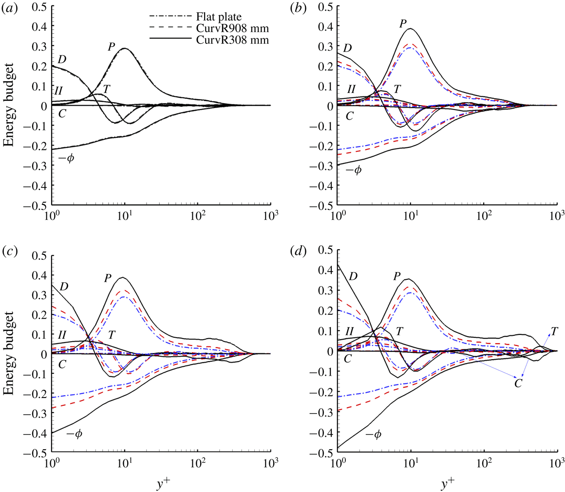
The TKE budget profiles of the flat plate case and concave cases at different streamwise locations: (a)  $x/\unicode[STIX]{x1D6FF}_{0}=-2.42$ , (b)  $x/\unicode[STIX]{x1D6FF}_{0}=0.81$ , (c)  $x/\unicode[STIX]{x1D6FF}_{0}=5.65$ and (d)  $x/\unicode[STIX]{x1D6FF}_{0}=10.50$ . Dash-dotted line represents the flat plate case. Dashed line represents the CurvR908mm case. Solid line represents the CurvR308mm case.

Figure 30.

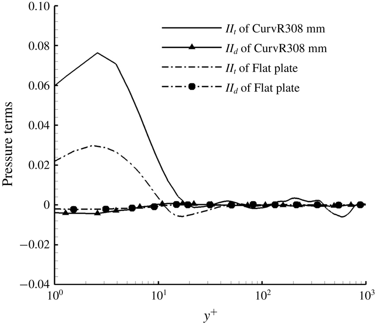
Comparison of pressure terms of flat plate case and CurvR308mm case at $x/\unicode[STIX]{x1D6FF}_{0}=10.50$ .

Figure 31.

The PDF of the dilatation is computed statistically in ( $x,y$ ) planes corresponding to different wall-normal locations $y/\unicode[STIX]{x1D6FF}_{0}\in$ (0.1, 0.5) and $x/\unicode[STIX]{x1D6FF}_{0}\in$ (0.81, 10.50) without scaling and with density scaling.

Figure 32.

Profiles of the turbulent Mach number $M_{t}$ (a,b) and the fluctuating RMS Mach number $M^{\prime }$ (c,d) of the flat plate and concave cases at different streamwise locations: (a)  $x/\unicode[STIX]{x1D6FF}_{0}=0.81$ (▾), $x/\unicode[STIX]{x1D6FF}_{0}=5.65$ (▴) and $x/\unicode[STIX]{x1D6FF}_{0}=10.50$ (♦). Dash-dotted line represents the flat plate case. Dashed line represents the CurvR908mm case. Solid line represents the CurvR308mm case.

Figure 33.

Effective Mach number $M_{c,bl}$ over the flat plate and concave walls.

To further assess the boundary layer on the concave walls, TKE budgets are compared to the flat plate results at different streamwise locations, as shown in figure 29. At the location $x/\unicode[STIX]{x1D6FF}_{0}=-2.42$ upstream of the corner, there is no difference between the flat plate and the concave cases. TKE budgets all show behaviour typical of a boundary layer at zero pressure gradient in which production is balanced by dissipation over most of the boundary layer, as also described by Guarini et al. (Reference Guarini, Moser, Shariff and Wray2000) and Pirozzoli et al. (Reference Pirozzoli, Grasso and Gatski2004). Viscous diffusion is only important in the near-wall region. In the viscous sublayer, production becomes negligible and diffusion is balanced by dissipation.

At $x/\unicode[STIX]{x1D6FF}_{0}=0.81$ in the turning region, compared to the flat plate case, all terms in the concave cases increase in magnitude in the inner layer. The TKE production increases slightly in the outer layer ( $y^{+}\in [60,500]$ ). The pressure diffusion and dilatation $II$ terms in the TKE equation become apparent due to the APG caused by concave compression. The convection term $C$ at the boundary-layer edge falls to larger negative values, which means the convection from the boundary layer to the main stream is augmented. The TKE becomes higher from the interaction of the boundary layer with the main stream at $x/\unicode[STIX]{x1D6FF}_{0}=0.81$ .

At $x/\unicode[STIX]{x1D6FF}_{0}=5.65$ , all terms in the TKE budget equation are amplified for the concave cases, while the TKE budget terms in the inner layer increase in magnitude with curvature rate. In the outer layer where $y^{+}\in [100,600]$ , the dissipation increases with curvature rate while TKE production and TKE convection terms are amplified significantly. The production augmentation is basically balanced by a negative increment in convection, which means the turbulence produced in the outer layer is mainly convected away.

At $x/\unicode[STIX]{x1D6FF}_{0}=10.50$ , the production term of the CurvR308mm case becomes larger than that of the CurvR908mm case, especially in the outer layer $y^{+}\in [100,1000]$ . This also corresponds to the generation of the outer peak in the TKE profile for the CurvR308mm case. The TKE pressure diffusion ( $II_{t}$ ) and dilatation ( $II_{d}$ ) terms become more significant due to the APG caused by the concave wall. Here we consider the contribution of the pressure terms, $II_{t}$ and $II_{d}$ . Figure 30 shows a comparison of pressure terms at $x/\unicode[STIX]{x1D6FF}_{0}=10.50$ between the CurvR308mm case and the flat plate case. The pressure diffusion term is larger than the pressure dilatation term, which indicates that pressure diffusion effect plays a dominant role, instead of the explicit compressibility effect. The magnitude of the convection term increases significantly in the outer layer of the boundary layer while the dissipation is amplified slightly, which means local convection of turbulent energy is amplified for the CurvR308mm case. The transport term is also amplified at $x/\unicode[STIX]{x1D6FF}_{0}=10.50$ and participates in balancing the production.

6.1 Dilatation

To further assess the compressibility and curvature effects, the probability distribution function (PDF) of the dilatation term, $\unicode[STIX]{x1D6E9}=\unicode[STIX]{x2202}_{x}u+\unicode[STIX]{x2202}_{y}v+\unicode[STIX]{x2202}_{z}w$ , is computed. Figure 31 shows the PDF, which is computed by averaging over the range $y/\unicode[STIX]{x1D6FF}_{0}\in (0.1,0.5)$ and $x/\unicode[STIX]{x1D6FF}_{0}\in (0.81,10.50)$ . For the flat plate case the PDF is sharp and peaks at zero dilatation. However, on the concave walls, the PDF is wider and the peak shifts to negative values of dilatation. The latter effect can be explained from the continuity equation

(6.1) $$\begin{eqnarray}\frac{\unicode[STIX]{x2202}\unicode[STIX]{x1D70C}}{\unicode[STIX]{x2202}t}+\frac{\unicode[STIX]{x2202}\unicode[STIX]{x1D70C}u_{i}}{\unicode[STIX]{x2202}x_{i}}=\frac{\unicode[STIX]{x2202}\unicode[STIX]{x1D70C}}{\unicode[STIX]{x2202}t}+\unicode[STIX]{x1D735}\unicode[STIX]{x1D70C}\boldsymbol{\cdot }\boldsymbol{u}+\unicode[STIX]{x1D6E9}\unicode[STIX]{x1D70C}=0.\end{eqnarray}$$

Since $\unicode[STIX]{x1D735}\unicode[STIX]{x1D70C}\boldsymbol{\cdot }\boldsymbol{u}$ is always positive on the concave wall, for small fluctuations we expect the average $\unicode[STIX]{x1D6E9}$ to be negative. With increasing curvature the PDF of dilatation becomes more skewed, with more extreme events of large negative dilation, which for higher Mach numbers or stronger curvatures may lead to the formation of eddy shocklets. A scaling of PDF $\bar{\unicode[STIX]{x1D70C}}\unicode[STIX]{x1D6E9}$ using the mean density $\bar{\unicode[STIX]{x1D70C}}$ has previously been used to collapse different PDF curves, as discussed by Lagha et al. (Reference Lagha, Kim, Eldredge and Zhong2011). Figure 31 includes the density scaling PDF; however, the distribution is similar to the non-scaled data for all the concave cases.

6.2 Turbulent Mach number

Turbulent Mach number $M_{t}=\sqrt{\overline{u_{j}^{\prime }u_{j}^{\prime }}}/\bar{c}$ profiles are shown in figure 32(a,b) at different streamwise locations for $x/\unicode[STIX]{x1D6FF}_{0}=0.81$ , 5.65 and 10.50. In addition to the turbulent Mach number, we also examine the RMS values of the local Mach number, the fluctuating Mach number $M^{\prime }$ ( $=(\overline{M^{2}}-\overline{M}^{2})^{1/2}$ ), which is different in compressible flows. The fluctuating Mach number profiles are shown in figure 32(c,d). For the flat plate case, the turbulent Mach number is no more than 0.3 and its maximum peak is located near to the wall. For the concave cases, turbulent Mach number starts to build a second peak which moves away from the wall, as seen in figure 32(a,b). The profiles of $M_{t}$ and $M^{\prime }$ exhibit a similar character with the outer peak shown in figure 27. In figure 32(c,d), the maximum of the second peak of the fluctuating Mach number exceeds 0.3 which suggests that the compressibility is approaching the borderline of Morkovin (Reference Morkovin and Favre1962).

6.3 Effective Mach number

An effective Mach number has also been proposed (Sandham Reference Sandham2016) to evaluate the compressibility effects of a turbulent boundary layer with APG variation from zero to separation, given by

(6.2) $$\begin{eqnarray}M_{c,bl}=\frac{\unicode[STIX]{x0394}U_{VD}^{+}}{U_{e}^{+}}\frac{M_{\infty }}{\left(1+a_{w}/a_{\infty }\right)}=\frac{\unicode[STIX]{x0394}U_{VD}^{+}}{U_{e}^{+}}\frac{M_{\infty }}{\left(1+\sqrt{T_{w}/T_{\infty }}\right)},\end{eqnarray}$$

where $a$ is the local speed of sound. Here, $\unicode[STIX]{x0394}U_{VD}^{+}$ refers to the van Driest-transformed velocity increment in the wake region compared to log law using the van Driest profile at $y=\unicode[STIX]{x1D6FF}$ , i.e.

(6.3) $$\begin{eqnarray}\unicode[STIX]{x0394}U_{VD}^{+}=U_{e,\unicode[STIX]{x1D6FF}}^{+}-\left(\frac{1}{\unicode[STIX]{x1D705}}\ln \unicode[STIX]{x1D6FF}_{}^{+}+b\right),\end{eqnarray}$$

where $U_{e,\unicode[STIX]{x1D6FF}}^{+}$ is the van Driest-transformed velocity at $y=\unicode[STIX]{x1D6FF}$ . The calculated results are shown in figure 33. The level of 0.3 is usually taken as the threshold above which compressibility effects are expected to be significant. We see that this is not reached for the CurvR308mm case and the compressibility effect increases as curvature ratio increases. Recalling the analysis of the dilatations, turbulent Mach number and fluctuating Mach number, it is inferred that the compressibility for the current concave cases does not exceed the threshold; however, for larger curvature ratios than those in this paper, the compressibility effects probably need be considered in turbulence modelling, which needs further investigations.