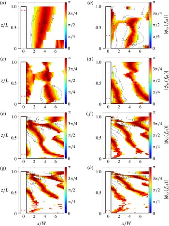
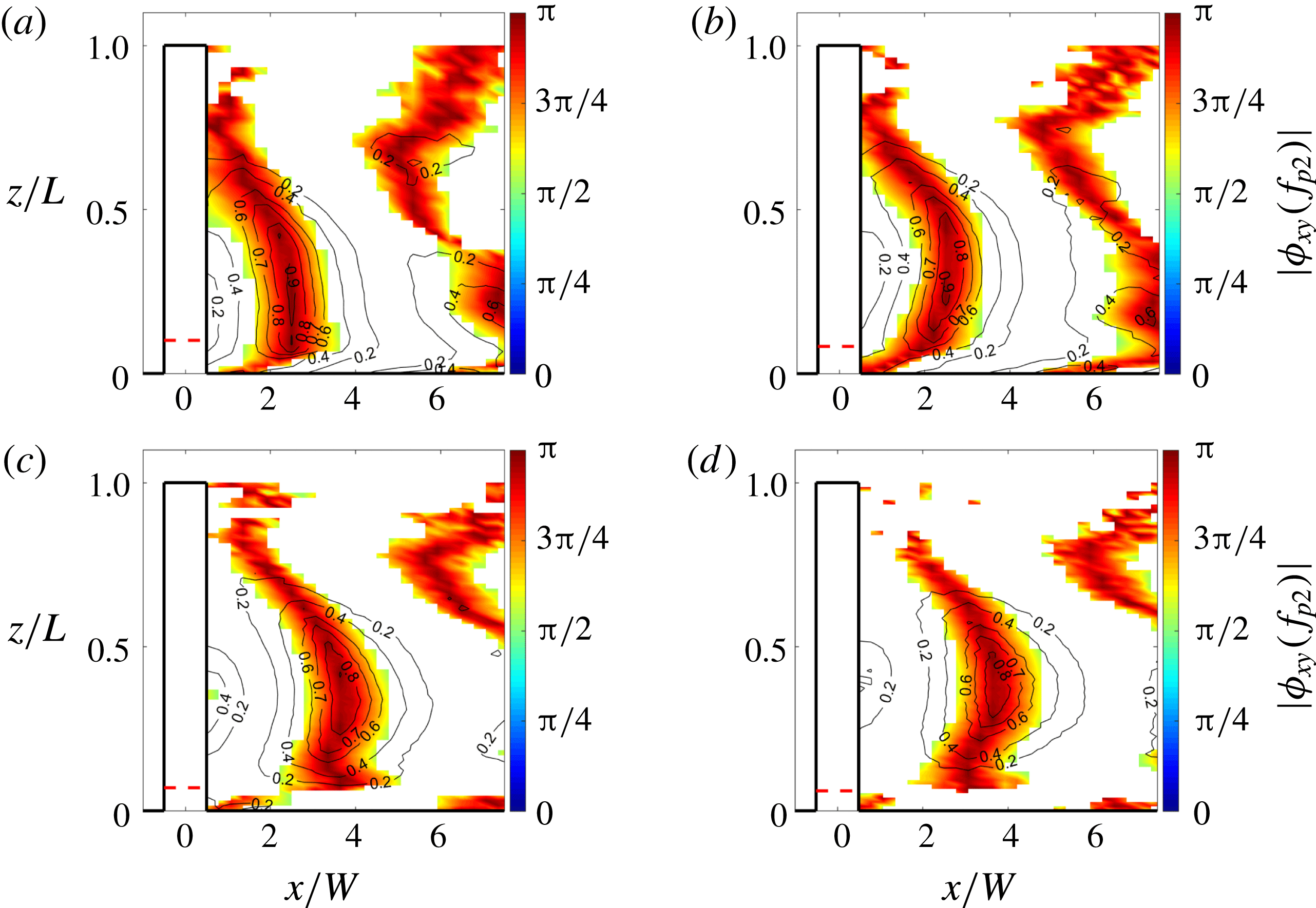
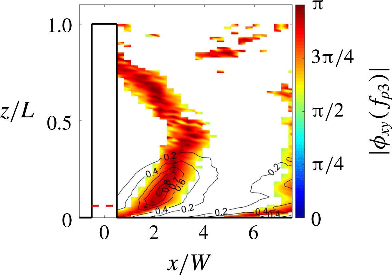
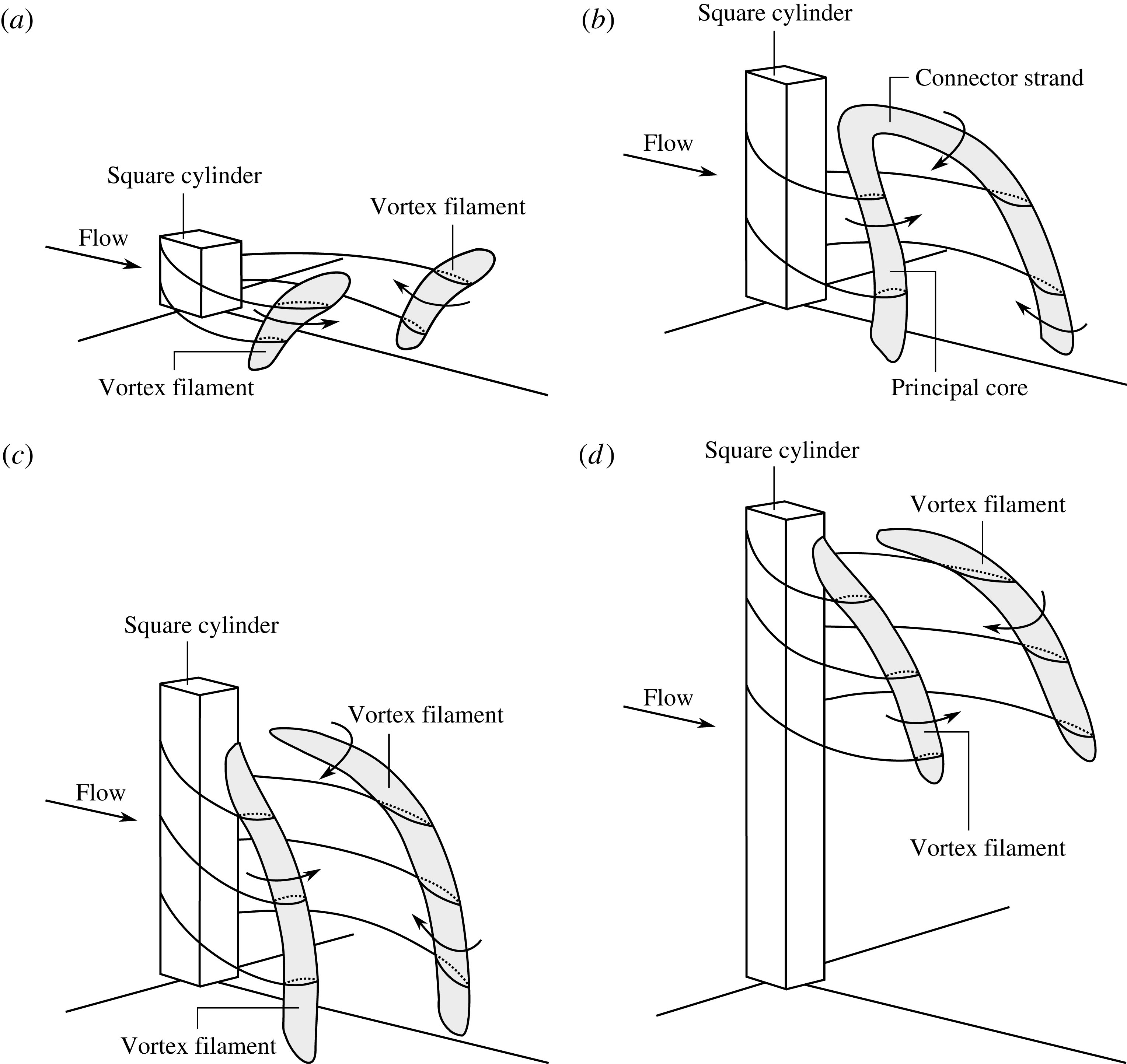
1 Introduction
Finite wall-mounted cylinders (FWMCs) in cross-flow are fundamental flow analogues for many industrial applications, such as aircraft landing gear, train pantographs, automotive external mirrors and submarine appendages. Of particular interest is an understanding of the noise producing physics, as this will lead to the creation of quieter transportation systems and a reduction in environmental noise pollution, a known public health issue (Passchier-Vermeer & Passchier Reference Passchier-Vermeer and Passchier2000). This paper concentrates on the noise generated by square FWMCs, how it is affected by aspect ratio and the near-wake flow structures responsible for its generation.
The wake of square FWMCs varies significantly from its two-dimensional counterpart. In the two-dimensional case, the noise is generally characterised by an Aeolian tone that is caused by quasi-periodic von Kármán vortex shedding and the associated fluctuating surface pressures. Curle (Reference Curle1955) developed the well-known theory that relates unsteady surface pressure to radiated noise, which has been confirmed many times experimentally (Keefe Reference Keefe1961; Leclercq & Doolan Reference Leclercq and Doolan2009, for example). FWMCs have a three-dimensional wake that alters the fluctuating surface pressure distribution and hence the radiated noise. The key factors that influence this redistribution are the aspect ratio (
 $L/W$
, where
 $L$
is the length of the cylinder and
 $W$
is its width or side length),
 $\unicode[STIX]{x1D6FF}/W$
(where
 $\unicode[STIX]{x1D6FF}$
is the oncoming boundary layer height), the cylinder geometry and the Reynolds number, although the effect of the Reynolds number has been shown to be small, especially for square FWMCs with fixed separation points (Bourgeois, Sattari & Martinuzzi Reference Bourgeois, Sattari and Martinuzzi2011). The wake and noise generation literature for square and circular FWMCs has recently been reviewed by Porteous, Moreau & Doolan (Reference Porteous, Moreau and Doolan2014); a concise updated review for square FWMCs will be presented below.
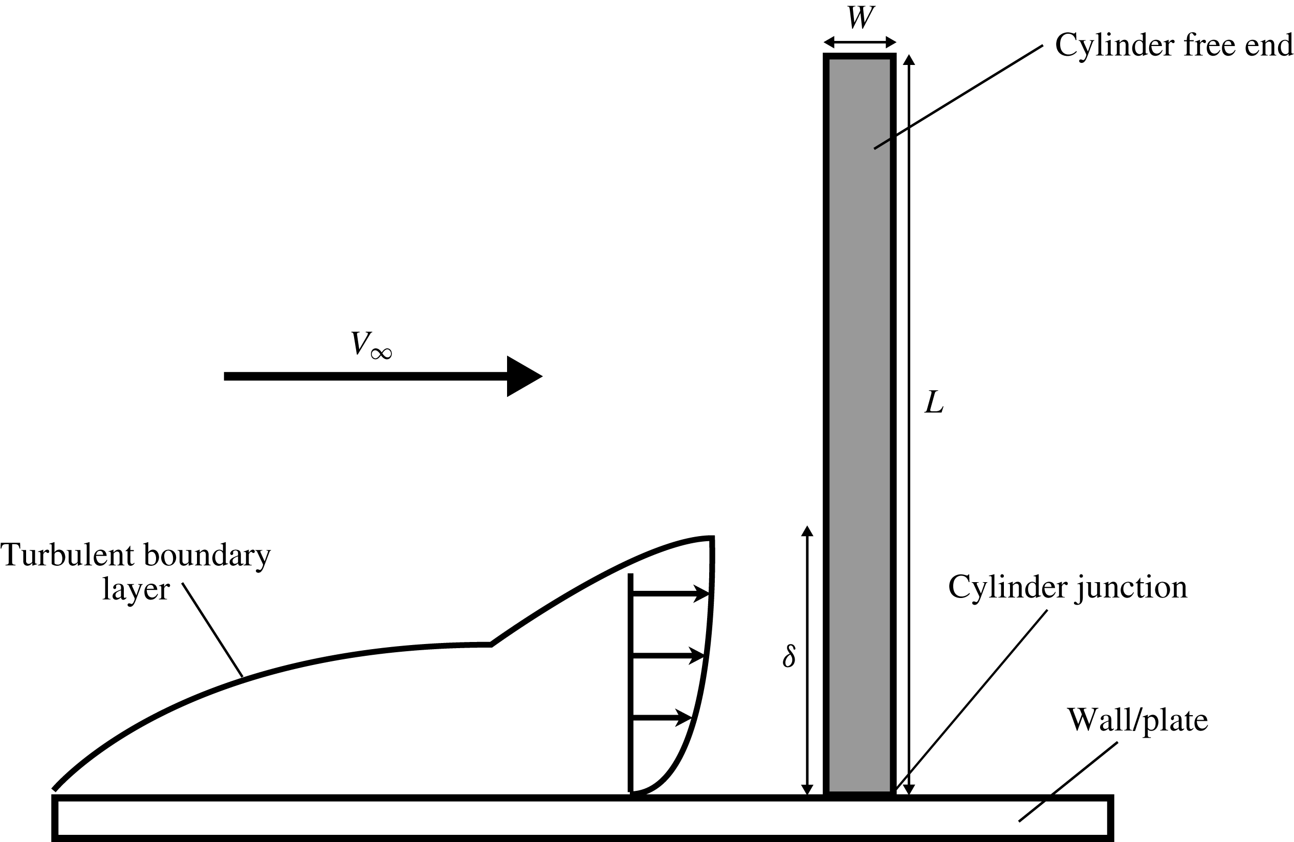
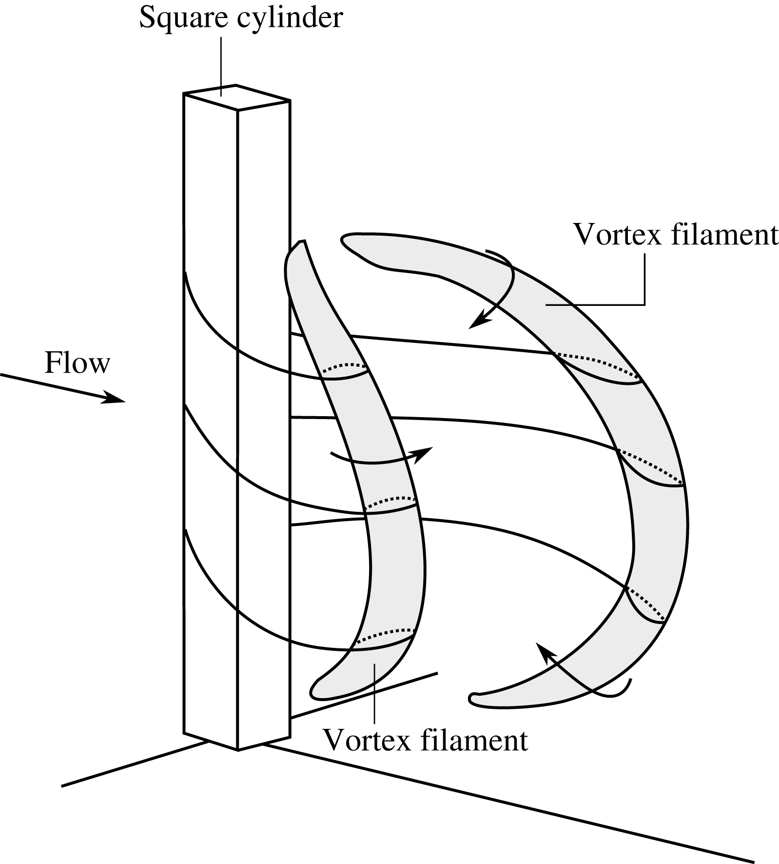
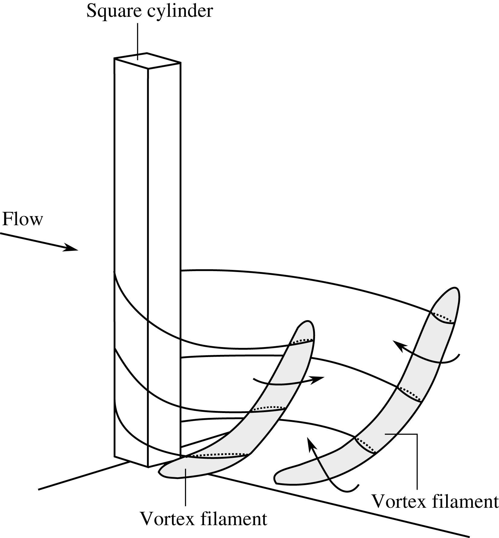
The square FWMC wake flow is influenced by the combined effects of the oncoming boundary layer in the junction region and the downwash created by flow over the free-end or tip region (figure 1). Sakamoto & Arie (Reference Sakamoto and Arie1983) first observed arch-type (or symmetric) vortex shedding occurring behind square FWMCs for
 $L/W\lesssim 2$
. Sakamoto & Oiwake (Reference Sakamoto and Oiwake1984) also noticed that the root-mean-square lift fluctuation decreases rapidly when arch-type vortex shedding is present.
A square FWMC mounted to a flat wall with width
 $W$
and span
 $L$
subject to a flow with free-stream velocity
 $V_{\infty }$
and an incoming boundary layer height of
 $\unicode[STIX]{x1D6FF}$
.

Wang et al. (Reference Wang, Zhou, Chan and Lam2006) experimentally studied the effect of boundary layer height on the square FWMC wake. The oncoming boundary layer height was shown to affect the amount of upwash from the junction region. Consequently, the influence of the boundary layer was felt outside of the junction region and influenced the wake along the entire span. The effect of aspect ratio (
 $3\leqslant L/W\leqslant 11$
) was investigated in detail for a fixed boundary layer height (
 $\unicode[STIX]{x1D6FF}/W=1.35$
) by Wang & Zhou (Reference Wang and Zhou2009). This work proposed a unified model for vortex shedding based on an arch-type model: the tip, base and spanwise vortices were considered as a single entity. The aspect ratio influenced the interaction between junction region upwash and tip region downwash, affecting the manner in which the arch vortex was shed into the wake. At low aspect ratios, strong interaction occurred, making the wake appear to be shed symmetrically; at high aspect ratios, the interaction weakened, allowing the arch to stagger, creating the appearance of non-symmetrical shedding.
Bourgeois et al. (Reference Bourgeois, Sattari and Martinuzzi2011) and Bourgeois, Noack & Martinuzzi (Reference Bourgeois, Noack and Martinuzzi2013) proposed a related ‘half-loop’ model, where vortex filaments are shed periodically and are linked with connector strands, leading to a fully connected alternating looped structure that is convected downstream. Hosseini, Bourgeois & Martinuzzi (Reference Hosseini, Bourgeois and Martinuzzi2013) investigated the wake for a square FWMC with
 $L/W=8$
with two boundary layer heights. Here, half-loop and full-loop wake structures were observed. A single shedding frequency was measured, which was taken as evidence that the wake structures were interconnected. The flow structures were bent towards either the free end and/or the junction depending on the boundary layer height.
Sattari, Bourgeois & Martinuzzi (Reference Sattari, Bourgeois and Martinuzzi2012) identified two modes of vortex shedding on a square FWMC with
 $L/W=4$
. The first, mode A, is anti-symmetric shedding that occurs during high-amplitude pressure fluctuations on the cylinder side face and is similar to von Kármán vortex shedding. Mode B, alternatively, is symmetrical vortex shedding during low-amplitude pressure fluctuations on the cylinder. Mode B occurs more frequently towards the free end, where downwash from the tip interacts with the vortex shedding process. Proper orthogonal decomposition (POD) analysis by Wang, Cao & Zhou (Reference Wang, Cao and Zhou2014) confirmed that symmetrical shedding occurs more often towards the free end, and anti-symmetrical shedding occurs in the mid-span.
The aeroacoustics of square FWMCs is much less studied than the wake, although the two are of course linked. King & Pfizenmaier (Reference King and Pfizenmaier2009) have provided the first experimental data for finite square cylinders from testing in a free jet (there was no wall junction in this study, only a free end). Here, two aspect ratios were tested:
 $L/W=16.7$
and
 $L/W=25$
. Strong vortex shedding noise was measured; however, instead of a single Aeolian tone, multiple tones were observed in the spectra. These additional tones were attributed to the additional flow structures generated at the tip of the cylinder, although no flow measurements were performed.
Becker et al. (Reference Becker, Hahn, Kaltenbacher and Lerch2008) performed a comprehensive experimental study of a square FWMC with
 $L/W=6$
. The radiated sound was dipolelike, although with the dipole lobes shifted upstream. Wall-pressure fluctuations were not evenly distributed along the cylinder, confirming the link between the three-dimensionality of the wake and the noise source (wall pressure). In general, the frequency of the Aeolian tone was found to be lower than what would be expected from an equivalent two-dimensional square cylinder. Moreover, the flow over the free tip was shown to influence the development of the vortex wake.
Moreau & Doolan (Reference Moreau and Doolan2013) carried out a comprehensive experimental aeroacoustic investigation of square FWMCs for
 $0.97\leqslant L/W\leqslant 13.6$
. They confirmed the dipolelike nature of the acoustic field and found that it scaled with the sixth power of the Mach number. Importantly, a cellular vortex shedding structure was observed, which was dependent on the aspect ratio. For
 $L/W\geqslant 8.7$
, two vortex cells were observed and two Aeolian tones were recorded. This is an interesting and important result because it confirms a cellular variation in the wake, which does not agree with the wake models put forward by Wang & Zhou (Reference Wang and Zhou2009), Bourgeois et al. (Reference Bourgeois, Sattari and Martinuzzi2011, Reference Bourgeois, Noack and Martinuzzi2013) and Sattari et al. (Reference Sattari, Bourgeois and Martinuzzi2012); these wake models are based on a continuous vortex structure across the span, rather than the cellular one observed by Moreau & Doolan (Reference Moreau and Doolan2013).
In order to shed additional light on the noise producing physics of square FWMCs, new experimental results are presented here, for a very wide range of aspect ratios (
 $0.29\leqslant L/W\leqslant 22.9$
). Multiple vortex shedding tones are comprehensively analysed and related to the wake structures using a novel method that utilises both acoustic and wake velocity signals. The specific aims of this paper are to (1) comprehensively characterise the noise produced by square FWMCs, (2) determine the flow patterns associated with FWMC wakes for different aspect ratios, (3) measure the salient flow parameters around the FWMC for differing aspect ratios and (4) relate these patterns and features to the flow-induced noise. The results presented in this paper are the first to comprehensively demonstrate the highly nonlinear behaviour of FWMC noise with changing aspect ratio due to the complicated three-dimensional wake structure of the FWMC. Furthermore, this is also the only study to investigate the wake dynamics of square FWMCs for
 $L/W\geqslant 14$
.
2 Experimental methodology
2.1 Facility description
Flow-induced noise and wake velocity measurements were taken in the University of Adelaide’s anechoic wind tunnel (AWT). In this wind tunnel, air is supplied via a 3 kW centrifugal fan (Fantech model no. 27B B1) located above the test chamber. The air is passed through an 8 m long silencer. The silencer has five
 $90^{\circ }$
corners (each with turning vanes installed to minimise pressure loss) and is lined with 200 mm thick acoustic foam (BaryNal). The flow then enters a circular settling chamber where it passes through a series of fine wire mesh gauze screens and a honeycomb section. After exiting the settling chamber, the air flows through a rectangular contraction with a contraction ratio of 3.67 and an outlet with a height of 75 mm (in the ‘
 $y$
’ direction) and a width of 275 mm (in the ‘
 $z$
’ direction). The turbulence intensity at the maximum contraction outlet velocity of
 $38~\text{m}~\text{s}^{-1}$
is approximately 0.4 %.
The flow is exhausted into an anechoic chamber with internal dimensions of
 $1.4~\text{m}\times 1.4~\text{m}\times 1.6~\text{m}$
. The walls of this chamber are lined with pyramid shaped foam wedges (with a height of 295 mm and a base width of
 $100~\text{mm}\times 100~\text{mm}$
) which provide a near anechoic environment above 250 Hz. A funnel shaped collector is located approximately 800 mm from the exit plane of the contraction outlet to eliminate air recirculation within the chamber, making the area outside of the jet flow near quiescent.
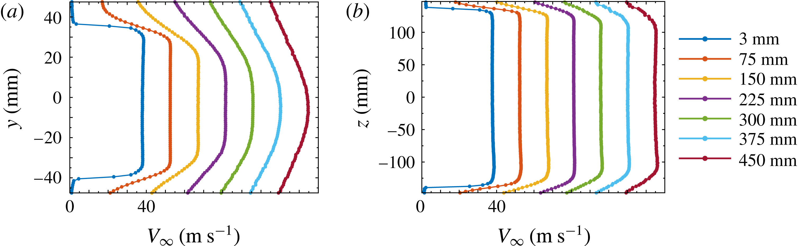
Figure 2 shows the profiles of the mean velocity across the exit plane of the contraction outlet in the
 $y$
and
 $z$
directions at
 $V_{\infty }=38~\text{m}~\text{s}^{-1}$
. The results are repeated for various downstream stations, starting from the jet exit plane at
 $x=0$
and repeating every 75 mm. The profiles show that the outlet flow is highly uniform at locations up to 150 mm away from the exit plane in both the
 $y$
and
 $z$
directions.
The mean velocity profiles across the mid-plane of the contraction outlet at various downstream stations in (a) the
 $y$
direction and (b) the
 $z$
direction at
 $V_{\infty }=38~\text{m}~\text{s}^{-1}$
. Each profile (starting from
 $x=3~\text{mm}$
) is displaced by
 $15~\text{m}~\text{s}^{-1}$
from the previous profile.

2.2 Cylinder test rig
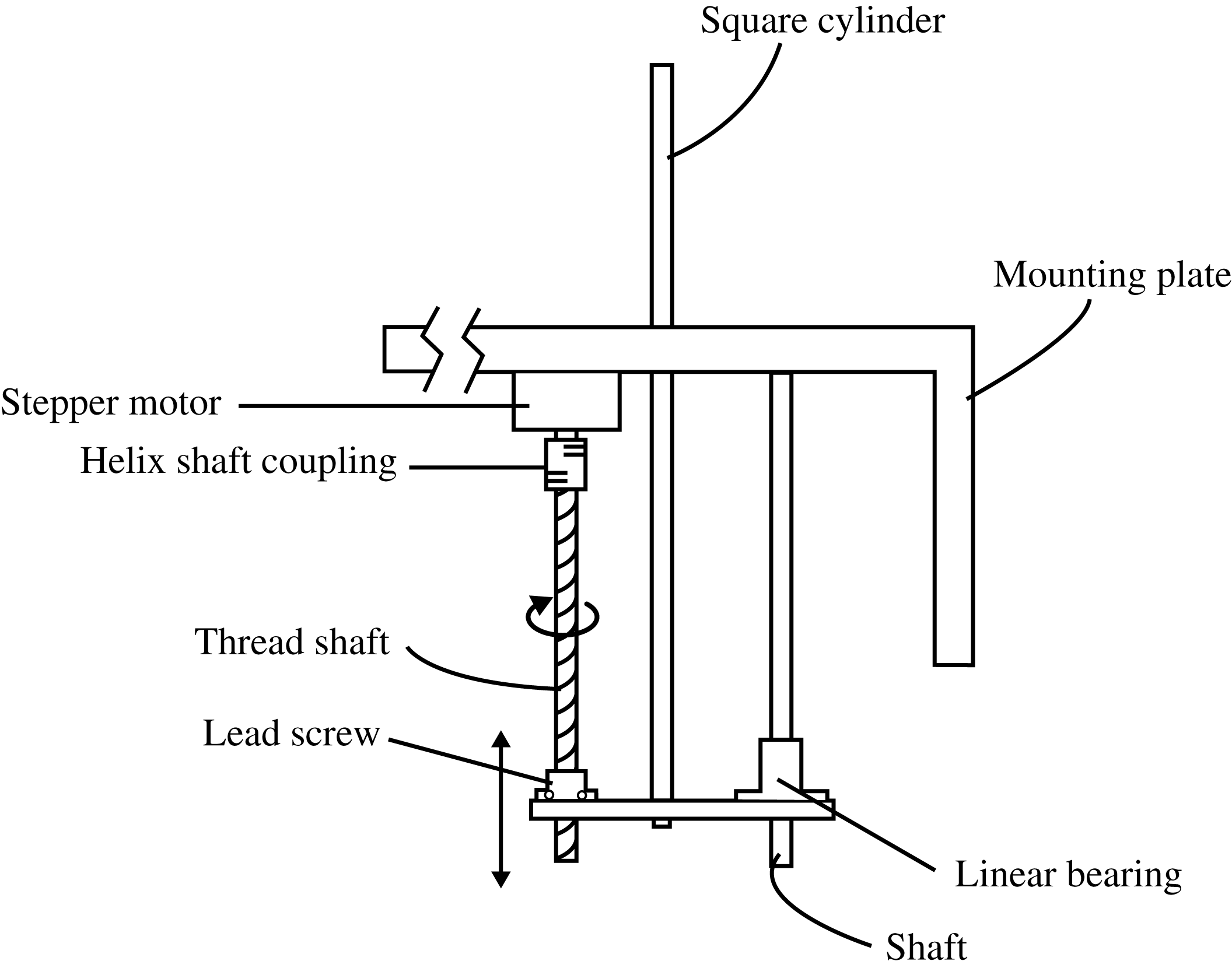
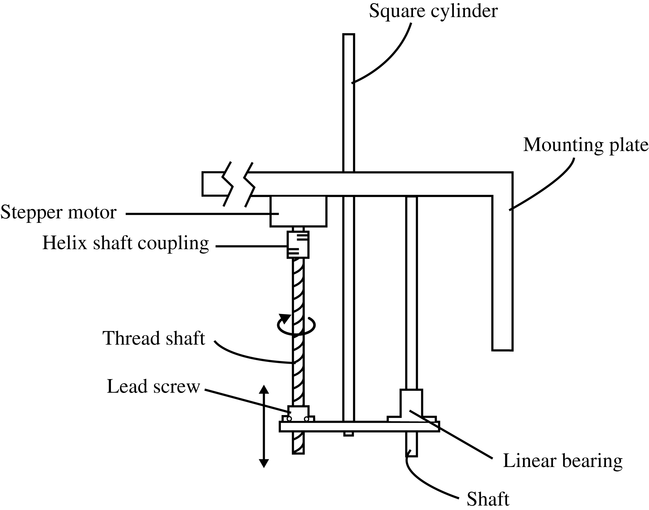
A test rig was designed to automatically change the aspect ratio of the square cylinder in small increments. A schematic of the rig is shown in figure 3. A stepper motor is used to rotate a 300 mm threaded shaft with an 8 mm pitch via a helical shaft coupling. As the threaded shaft rotates, a lead screw transfers the rotational motion into linear motion. The lead screw is fastened onto a small acrylic plate, where a 300 mm long square cylinder with a width of 7 mm is mounted at one end. The cylinder is driven linearly through a square hole in a flat plate made from 10 mm thick aluminium. The aluminium plate measures 300 mm in the streamwise (‘
 $x$
’) direction and 150 mm in the cross-stream (‘
 $y$
’) direction, while the hole is located in the centre of the plate at a position of 43 mm downstream of the jet exit plane. The maximum wetted length of the cylinder is 160 mm. The flat plate has a
 $90^{\circ }$
elbow and is mounted onto the contraction outlet flange such that the surface of the flat plate is flush with the inner sidewall of the contraction outlet. The acrylic plate that holds the lead screw and the cylinder is also connected to a linear bearing mounted on an additional aluminium shaft to ensure that the cylinder tracks smoothly. The stepper motor is controlled via an Arduino Uno microcontroller with an Adafruit Motor Shield. The uncertainty in the movement of the system is estimated to be
 $\pm 0.5/80=\pm 6.25\times 10^{-3}~\text{mm}$
for every 2 mm of linear motion.
A schematic of the rig constructed to automatically change the aspect ratio of the cylinder.
Unless otherwise stated, the coordinate system used in this paper has its origin at the junction of the FWMC, centred on the FWMC axis. The
 $x$
direction runs parallel with the free-stream flow, the
 $z$
direction runs parallel with the span of the FWMC and the
 $y$
direction runs orthogonal to both, in the cross-stream direction (figure 5).
2.3 Microphone measurements
Noise measurements were taken using a G.R.A.S.
 $1/4$
inch 40PH array microphone. The G.R.A.S. microphone has a flat frequency response (to within
 $\pm 1~\text{dB}$
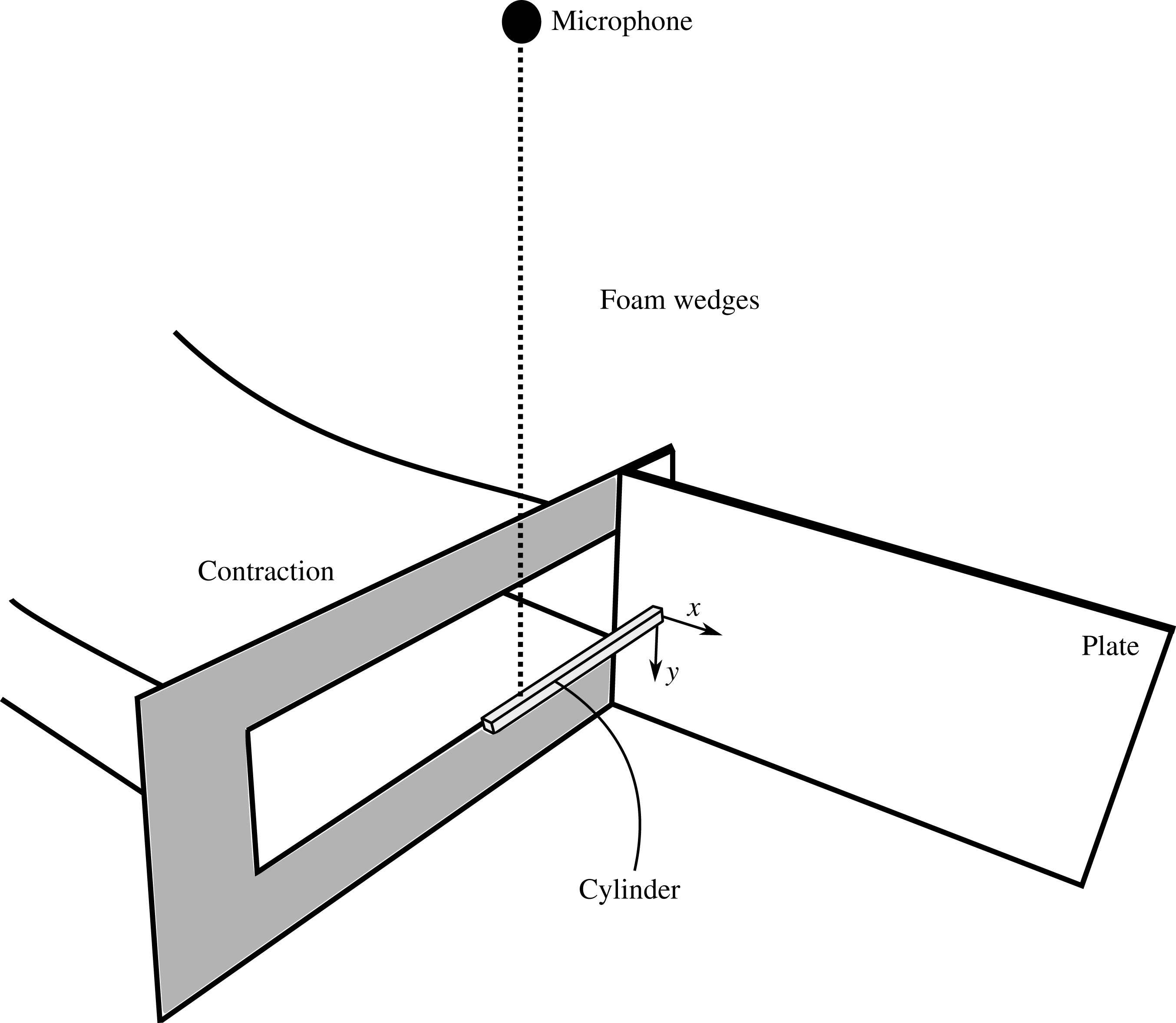
) from 20 Hz to 10 kHz. As shown in figure 4, the microphone was placed 0.5 m directly above the cylinder face, in the middle of the contraction; that is, at the location
 $(x,y,z)=(0,-500,137.5)$
in the above mentioned coordinate system. A National Instruments PXI Express Chassis (Model PXIe-1082) with PXIe-4499 simultaneous sample and hold ADC cards was used to collect microphone data. Each microphone measurement was sampled at 32 768 Hz for 30 s.
A schematic diagram of the experimental set-up for the microphone measurements.

2.4 Hot-wire anemometry
Hot-wire anemometry was used to perform a wake survey of the streamwise velocity downstream of the FWMCs. A Dantec Dynamics miniature hot-wire (model 55P16) controlled by an IFA300 Constant Temperature Anemometer system was used for the wake survey. Platinum plated tungsten wire was used as the sensing element, which had a diameter of
 $5~\unicode[STIX]{x03BC}\text{m}$
and a length of 1.25 mm. The hot-wire was held in an aerodynamic probe support constructed from a 3 mm diameter aluminium rod with a
 $90^{\circ }$
bend. This rod was secured to a
 $20~\text{mm}\times 20~\text{mm}$
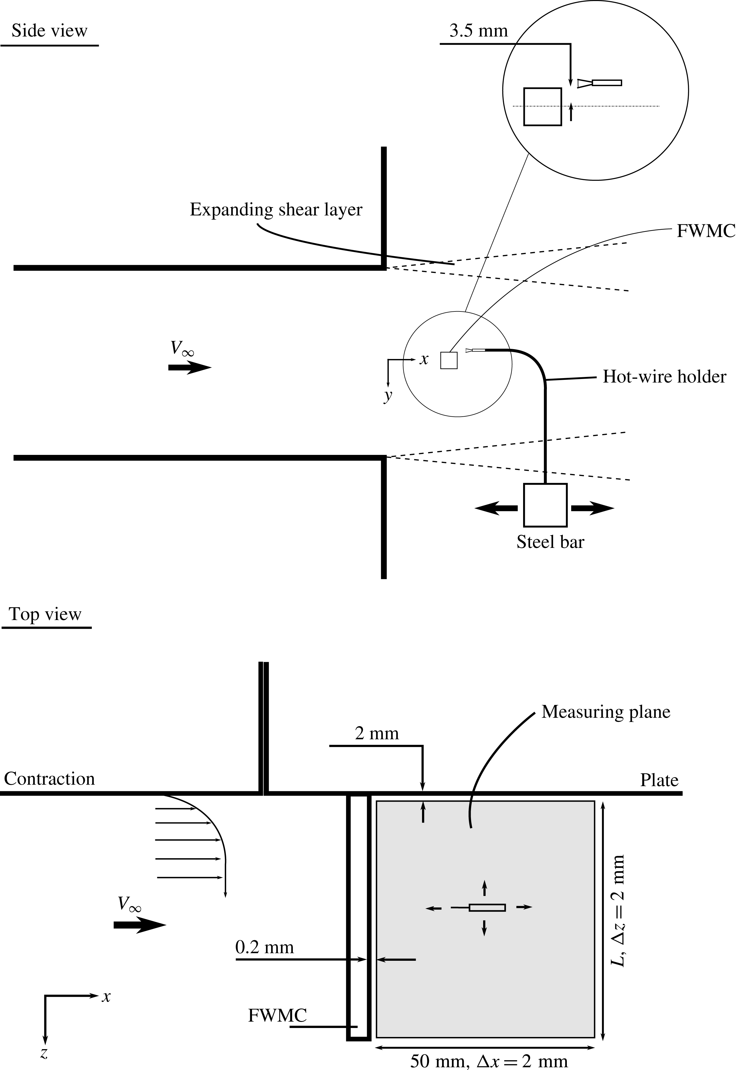
solid steel square bar that was mounted to the Dantec traverse, allowing the hot-wire to permit movement in all three directions. The mounting bar was kept out of the jet flow so that it did not introduce unwanted blockage effects. The set-up is illustrated in figure 5. As shown in figure 5, the hot-wire was oriented parallel to the cylinder width.
A schematic diagram of the experimental set-up for the hot-wire wake survey measurements.

The hot-wire was used to survey the wake behind different aspect ratio cylinders. The measurement plane behind each aspect ratio cylinder was a grid of points that measured 50 mm in the streamwise (
 $x$
) direction and the span of the cylinder in the spanwise (
 $z$
) direction. The measurement plane began at approximately 0.2 mm from the trailing edge of the cylinder and 2 mm above the surface of the plate (see figure 5). Additionally, the measurement plane was located at
 $y/W=0.6$
to avoid entering the reverse flow region in the cylinder wake. The grid increments were
 $\unicode[STIX]{x0394}x=\unicode[STIX]{x0394}z=2~\text{mm}$
. A hot-wire velocity record was taken at each node in the grid. The National Instruments PXI Express Chassis (Model PXIe-1082) with PXIe-4499 simultaneous sample and hold ADC cards was used to collect the hot-wire data. Each velocity record was sampled at 32 768 Hz for 15 s.
2.4.1 Calibration
The hot-wire was calibrated inside the AWT instead of a dedicated calibrator. This type of in situ calibration was preferred because the orientation of the hot-wire could be kept constant throughout the wind tunnel experiment. The hot-wire is weakly sensitive to the yaw and pitch components of the velocity (Perry Reference Perry1982). Therefore, if the hot-wire is calibrated in a nominal orientation, any deviation of the hot-wire position from this nominal orientation will be reflected in the relationship between the bridge voltage and the free-stream velocity (the calibration function). Hence, in situ calibration can eliminate probe misalignment error.
To create the calibration function, the hot-wire was placed on the traverse arm and positioned in the potential core of the wind tunnel (approximately 10 mm away from the contraction exit plane). The wind tunnel was then run at 11 different velocities ranging from 0 to
 $38~\text{m}~\text{s}^{-1}$
. The velocity of the tunnel was monitored using a Pitot tube connected to a 10 Torr MSK Baratron pressure transducer via 5 m long plastic tubing with an outer diameter of 5 mm. A fifth-degree polynomial was then fitted through the points to obtain the calculation function,
 $u=f(E)$
, relating the air velocity normal to the hot-wire (in this case the streamwise velocity),
 $u$
, to the bridge voltage,
 $E$
(Perry Reference Perry1982). Two calibration curves were generated for every cylinder wake that was surveyed: one curve before the survey and one directly after. These two calibration curves were averaged to obtain the final calibration curve for each cylinder wake survey.
Bruun (Reference Bruun1995) suggested that the maximum velocity used in the calibration routine should be as high as 1.5 times the maximum velocity used for experiments. Since the experimental free-stream velocity was set at
 $32~\text{m}~\text{s}^{-1}$
, the in situ calibration process described above did not provide an adequate calibration velocity range because the maximum speed of the tunnel was only
 $38~\text{m}~\text{s}^{-1}$
. To overcome this, velocities that lay beyond the calibration range were extrapolated from the calibration function. Extrapolation is not usually recommended because large linearisation errors can occur. However, in this study, a customised technique, known as the ‘modified extrapolation method’, was developed to minimise the linearisation errors for velocities beyond the calibration range, and is outlined below.
Suppose that a polynomial calibration curve,
 $u=f(E)$
, has been created between bridge voltages
 $E_{min}$
and
 $E_{max}$
, giving corresponding velocities of
 $u_{min}$
and
 $u_{max}$
. A voltage
 $E_{1}>E_{max}$
is converted to a velocity by first using the original transfer function,
 $u_{a}=f(E_{1})$
. A second data reduction is then performed by calculating the derivative of the transfer function,
 $B=\unicode[STIX]{x2202}f(E)/\unicode[STIX]{x2202}E|_{E=E_{max}}$
, at
 $E=E_{max}$
. The second velocity,
 $u_{b}$
, is calculated as
 $u_{b}=B(E_{1}-E_{max})+u_{max}$
. The final reduced velocity is given as the average of
 $u_{a}$
and
 $u_{b}$
.
This procedure was tested outside the wind tunnel in a TSI manual velocity calibrator (Model 1128). A calibration was performed between velocities of
 $0$
and
 $60~\text{m}~\text{s}^{-1}$
. The calibration curve, however, was only generated using points between 2 and
 $38~\text{m}~\text{s}^{-1}$
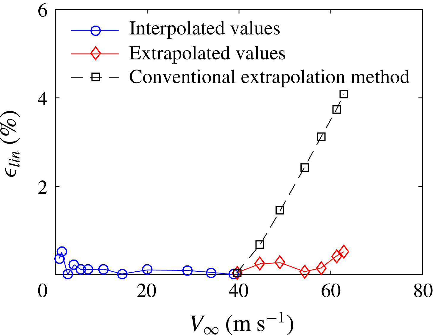
, simulating an AWT calibration. Velocities that lay outside this range were reduced using the extrapolation procedure described above. The extrapolated relative linearisation error,
 $\unicode[STIX]{x1D716}_{lin}$
, calculated as the difference between the extrapolated values and the true values normalised by their velocity, is shown in figure 6. This figure also shows the relative linearisation error for velocities that lie in the calibration range. By using the extrapolation technique described above, the linearisation errors are reduced to levels that are comparable to velocities that lie inside the calibration range. The errors associated with conventional extrapolation techniques, i.e. simply using the original transfer function in an extended domain, are also shown. By comparison, the linearisation errors associated with the conventional extrapolation technique are much higher than those of the modified extrapolation technique used in this study.
The linearisation error of the hot-wire using the modified extrapolation technique.

2.4.2 Sources of experimental error in the hot-wire measurements
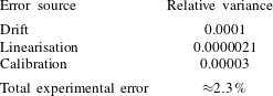
There were several sources of experimental error during the hot-wire experiments. These included errors associated with hot-wire drift, temperature variations, linearisation, digital quantisation, probe alignment and calibration error. Table 1 summarises the uncertainty of each contribution expressed as a relative variance (the relative standard deviation squared) based on an assumed probability distribution of each error. The methodology used to calculate these errors can be found in Porteous (Reference Porteous2016). This analysis estimated that the errors associated with temperature, probe misalignment and quantisation were negligible.
A summary of the major contributors to hot-wire measurement error.
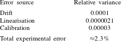
The total experimental error of a hot-wire velocity measurement was calculated using the law of propagation of errors. According to Lira (Reference Lira2002), by assuming that all sources of error are uncorrelated, the total experimental error of a single hot-wire measurement can be calculated using
 $$\begin{eqnarray}\unicode[STIX]{x1D716}_{total}=2\sqrt{\sum \frac{\text{var}_{i}(u)}{\mathop{V}_{\infty }^{2}}},\end{eqnarray}$$
where
 $\text{var}_{i}(u)/V_{\infty }^{2}$
is the relative variance of the
 $i$
th source of error. Table 1 summarises the magnitude of experimental sources of error discussed previously. It should be noted that the temperature error, bit error and probe misalignment error were assumed to be 0 % (Porteous Reference Porteous2016). The total experimental error was estimated as 2.3 %. There was one exception: for
 $L/W=10$
, the larger drift error causes the velocity uncertainty to increase to a maximum of 14 %.
2.4.3 Error in regions of high turbulence intensity
The final error type that will be discussed is the error caused when the hot-wire measures in regions where the turbulence intensity,
 $T.I.=\unicode[STIX]{x1D70E}/V_{\infty }>0.3$
. This error is different from those described above because it is a source that causes averaging errors in statistical estimates rather than an uncertainty at any one individual data point.
When a hot-wire is placed in a highly turbulent region, a combination of heat transfer nonlinearities and quadratic nonlinearities occurs due to the transverse components of velocity (Perry Reference Perry1982). As well as the streamwise component of velocity, transverse components of velocity will also add to the heat transfer from the wire, essentially raising the effective cooling velocity. Bradbury (Reference Bradbury1976) modelled the effect of transverse components of velocity. In his analysis, the effective cooling velocity,
 $V_{e}$
, is given by the Pythagorean sum of two velocity components,
 $u$
(in the streamwise direction) and
 $v$
(in the transverse direction), that are normal to the wire,
 $$\begin{eqnarray}V_{e}=(u^{2}+v^{2})^{0.5}.\end{eqnarray}$$
The probability density function of the turbulence,
 $p(u,v)$
, is assumed to be Gaussian with a streamwise mean velocity and variance of
 $V_{\infty }$
and
 $\unicode[STIX]{x1D70E}^{2}$
respectively and a transverse mean velocity and variance of 0 and
 $K^{2}\unicode[STIX]{x1D70E}^{2}$
respectively, where
 $K$
is a scalar constant. Then, according to Bradbury (Reference Bradbury1976), the apparent mean velocity,
 $V_{a}$
, sensed by the wire immersed in the turbulent velocity field is given by
 $$\begin{eqnarray}V_{a}=\iint V_{e}p(u,v)\,\text{d}u\,\text{d}v=\frac{1}{2\unicode[STIX]{x03C0}K\unicode[STIX]{x1D70E}^{2}}\iint (u^{2}+v^{2})^{0.5}\text{e}^{-(u-V_{\infty })^{2}/2\unicode[STIX]{x1D70E}^{2}}\text{e}^{-v^{2}/2K^{2}\unicode[STIX]{x1D70E}^{2}}\,\text{d}u\,\text{d}v.\end{eqnarray}$$
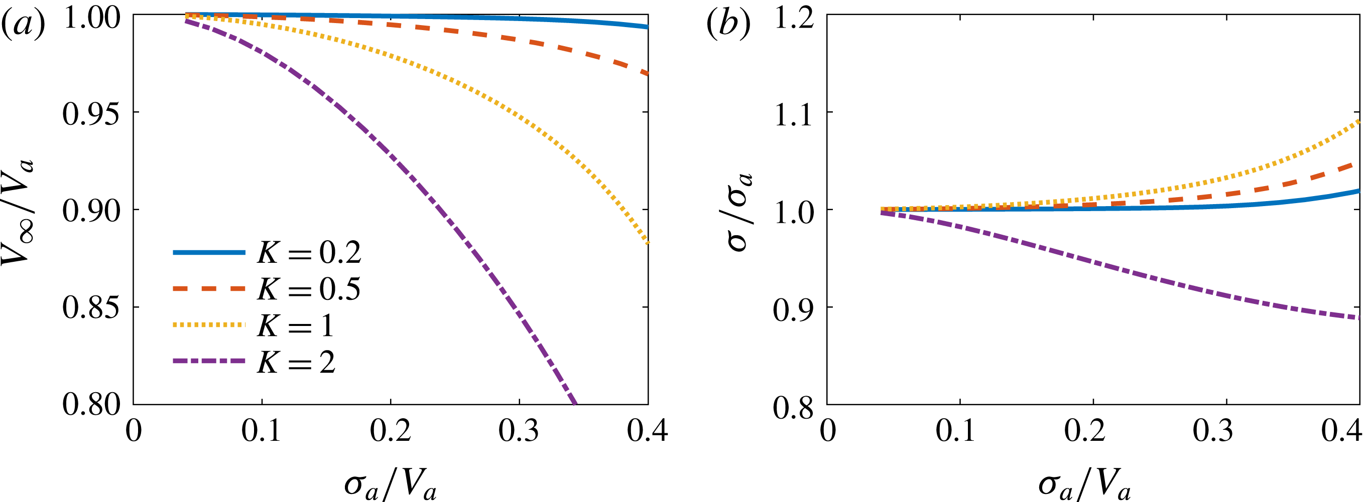
Figure 7(a,b) presents the ratio of the actual streamwise velocity to the apparent mean velocity,
 $V_{\infty }/V_{a}$
, and the ratio of the actual streamwise turbulence to the apparent streamwise turbulence
 $\unicode[STIX]{x1D70E}/\unicode[STIX]{x1D70E}_{a}$
, sensed by a hot-wire as a function of the apparent turbulence intensity of the velocity field,
 $\unicode[STIX]{x1D70E}_{a}/V_{a}$
, using (2.3). It is observed that as the apparent turbulence intensity increases, the apparent velocity deviates significantly from the true velocity. Similarly, for the apparent turbulence intensity, there is more deviation the higher the turbulence is, although, surprisingly, the effect is less severe. For the orientation of the hot-wire in the current experiments, the most important components of velocity are the streamwise components and the spanwise components that act parallel to the span of the cylinder. Wang & Zhou (Reference Wang and Zhou2009) and Rostamy et al. (Reference Rostamy, Sumner, Bergstrom and Bugg2012) showed that the streamwise and spanwise components of the fluctuating velocity in the free end and junction of the square FWMC wake have approximately the same order of magnitude. This corresponds to a value of
 $K=1$
in (2.3). From the turbulence model, the error in the measured mean velocity would be approximately 8 % at a longitudinal turbulence level of
 $\unicode[STIX]{x1D70E}=0.35$
. The error in the measured turbulence intensity would be approximately 5 % at the same turbulence level.
(a) The ratio of the true mean velocity to the apparent mean velocity,
 $V_{\infty }/V_{a}$
, and (b) the ratio of the true velocity turbulence to the apparent velocity turbulence,
 $\unicode[STIX]{x1D70E}/\unicode[STIX]{x1D70E}_{a}$
, both as a function of the apparent turbulence intensity,
 $\unicode[STIX]{x1D70E}_{a}/V_{a}$
, and degree of homogeneity of that turbulence that the hot-wire is immersed in,
 $K$
.

2.5 Test conditions
The experiments conducted in the AWT were performed at a free-stream velocity of
 $V_{\infty }=32~\text{m}~\text{s}^{-1}$
, corresponding to a Reynolds number of
 $Re_{W}=V_{\infty }W/\unicode[STIX]{x1D708}=1.4\times 10^{4}$
. The cylinder rig was used to incrementally change the aspect ratio in the range from
 $L/W=0.29$
to
 $L/W=22.9$
. The size of each increment was
 $\unicode[STIX]{x0394}L/W=0.29$
(2 mm in length), which yielded a total of 80 different aspect ratio cylinders. For the hot-wire wake surveys, a subset of eight different aspect ratio FWMCs were used. These aspect ratios were
 $L/W=1.4$
, 4.3, 7.1, 10.0, 12.9, 15.7, 18.6 and 21.4.
2.6 Incoming wall boundary layer characteristics
To characterise the incoming flow conditions, the wall boundary layer profile at the cylinder location (but with the cylinder removed) was measured in the AWT at
 $V_{\infty }=32~\text{m}~\text{s}^{-1}$
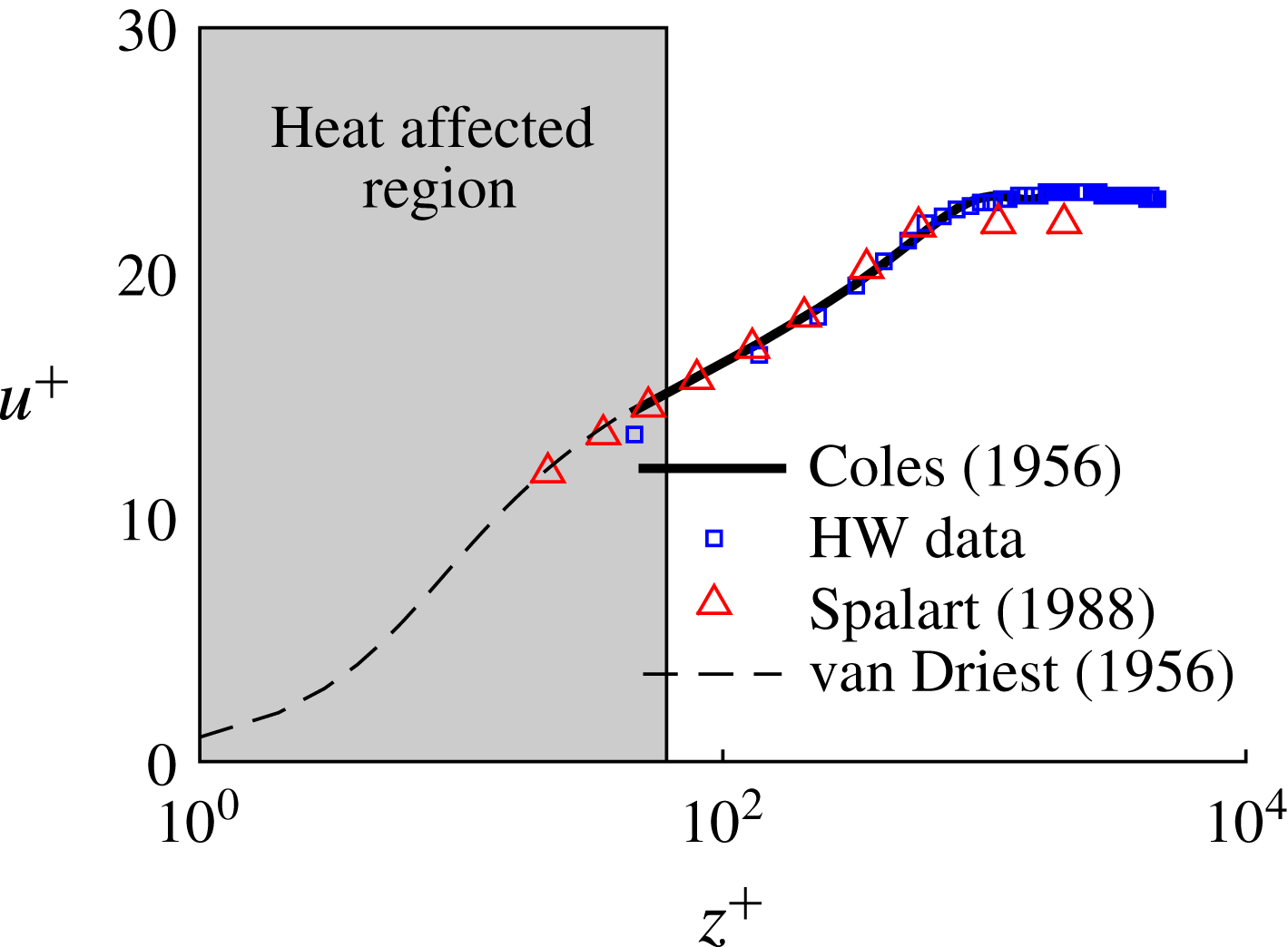
. Figure 8 shows the plate mean velocity boundary layer profile in wall units. In this figure,
 $z^{+}=zu_{\unicode[STIX]{x1D70F}}/\unicode[STIX]{x1D708}$
and
 $u^{+}=\overline{u(z)}/u_{\unicode[STIX]{x1D70F}}$
, where
 $u_{\unicode[STIX]{x1D70F}}$
is the friction velocity and
 $\unicode[STIX]{x1D708}$
is the kinematic viscosity of air. The friction velocity,
 $u_{\unicode[STIX]{x1D70F}}$
, was found by fitting the boundary layer mean velocity profiles to the law of the wake for turbulent boundary layers (Coles Reference Coles1956), described by
 $$\begin{eqnarray}u^{+}=\frac{1}{\unicode[STIX]{x1D705}}\log (z^{+})+C+\frac{2\unicode[STIX]{x1D6F1}}{\unicode[STIX]{x1D705}}\sin ^{2}\left(\frac{y\unicode[STIX]{x03C0}}{2\unicode[STIX]{x1D6FF}}\right),\end{eqnarray}$$
where
 $\unicode[STIX]{x1D705}=0.41$
and
 $C=5.0$
. In this equation, both the friction velocity,
 $u_{\unicode[STIX]{x1D70F}}$
, and the parameter
 $\unicode[STIX]{x1D6F1}$
(which describes the boundary layer streamwise pressure gradient) were found by varying them independently until the total variance between (2.4) and the measured data was minimised. It should be noted that when the hot-wire was close to the wall, heat transfer from the aluminium plate altered the temperature of the sensing element, which reduced the measured velocity. By observing the change in hot-wire bridge voltage as the hot-wire moved closer to the wall while the flow velocity was zero, the heat affected region was found to occur when
 $z/W\leqslant 0.3$
. Figure 8 compares the measured data with the fitted equation, and good agreement is observed. Figure 8 also compares the boundary layer with numerical data of Spalart (Reference Spalart1988) at a similar Reynolds number. Good agreement is achieved, which further confirms the turbulent nature of the boundary layer. For completeness, the near-wall solution of van Driest (Reference van Driest1956) is also given for
 $z^{+}<30$
.
Incoming boundary layer mean velocity profile in wall units. The profiles are compared with Coles law of the wake, van Driest’s near-wall solution (van Driest Reference van Driest1956) and results of Spalart (Reference Spalart1988).

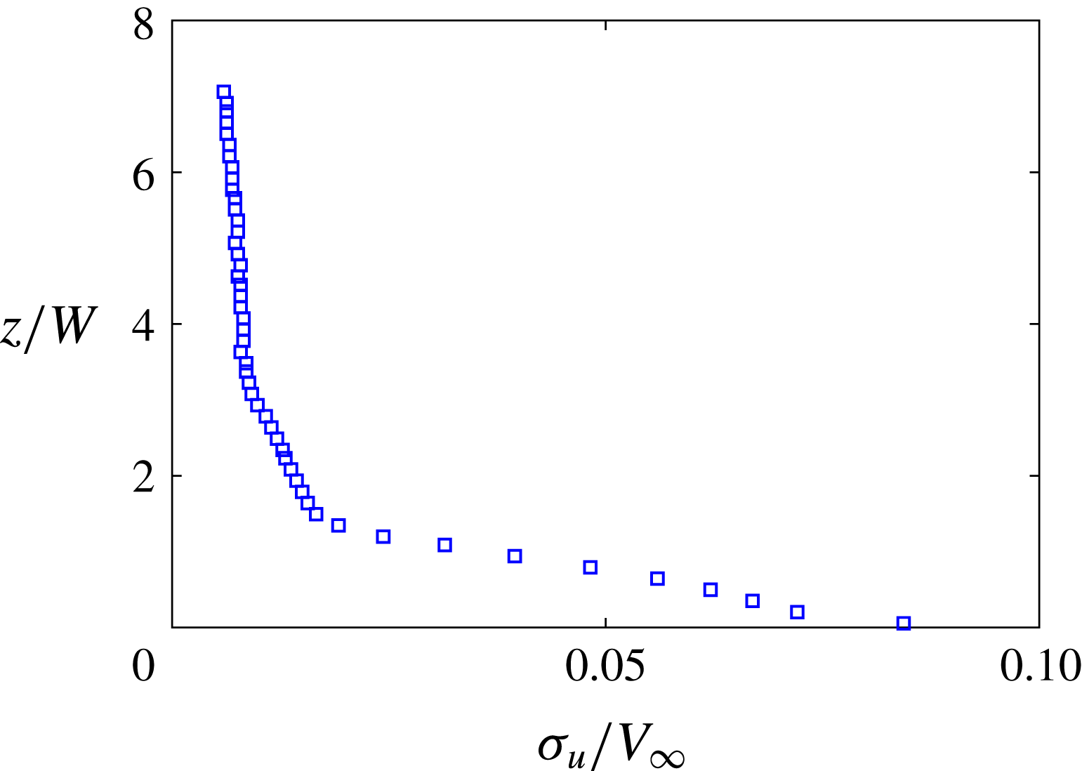
Figure 9 shows the wall normal turbulent intensity profile. The maximum turbulence intensity close to the wall is approximately
 $T.I.=8\,\%$
, which quickly reduces to the free-stream value of
 $T.I.=0.5\,\%$
by
 $z/W=4$
.
Incoming boundary layer turbulence intensity profile.

Table 2 shows the measured boundary layer integral properties, normalised by the appropriate scale. These include the boundary layer thickness,
 $\unicode[STIX]{x1D6FF}/W$
, the friction velocity,
 $u_{\unicode[STIX]{x1D70F}}/V_{\infty }$
, the parameter
 $\unicode[STIX]{x1D6F1}$
, the displacement thickness,
 $\unicode[STIX]{x1D6FF}^{\ast }/W$
, the momentum thickness,
 $\unicode[STIX]{x1D703}^{\ast }/W$
, the shape factor,
 $H=\unicode[STIX]{x1D6FF}^{\ast }/\unicode[STIX]{x1D703}^{\ast }$
, and the Reynolds number based on the momentum thickness,
 $Re_{\unicode[STIX]{x1D703}}=V_{\infty }\unicode[STIX]{x1D703}/\unicode[STIX]{x1D708}$
.
A comparison of key characteristics of the incoming boundary layer.

According to Wilcox (Reference Wilcox2006), a
 $\unicode[STIX]{x1D6F1}$
value of between 0 and 0.6, as given in table 2, indicates a near-zero streamwise pressure gradient. It is also shown in table 2 that the AWT boundary layer has a shape factor of
 $H=1.6$
. According to Pope (Reference Pope2000), a fully developed turbulent boundary layer has a shape factor of 1.3 while a laminar boundary layer has a shape factor of
 $H=2.6$
. This indicates that the incoming boundary layer is in a turbulent and nearly fully developed state.
3 Experimental results
3.1 Point microphone measurements
3.1.1 Overall sound pressure level
Curle’s theory (Curle Reference Curle1955) can be used to calculate the mean-square sound pressure,
 $\overline{p_{a}^{2}}$
, generated by an infinite square cylinder with width
 $W$
, undergoing vortex shedding at a Strouhal number,
 $St=fW/V_{\infty }$
(Phillips Reference Phillips1956),
 $$\begin{eqnarray}\overline{p_{a}^{2}}=\frac{V_{\infty }^{6}\unicode[STIX]{x1D70C}^{2}St^{2}\overline{C_{l}^{2}}LsW}{16c_{0}^{2}r^{2}},\end{eqnarray}$$
where
 $r$
is the distance from the cylinder axis to the far-field microphone (placed orthogonally to the cylinder axis) and the flow,
 $\overline{C_{l}^{2}}$
is the mean-square lift coefficient,
 $s$
is the spanwise correlation factor and
 $c_{0}$
is the speed of sound. Equation (3.1) demonstrates that the mean-square acoustic pressure is a function of three parameters that characterise the vortex shedding dynamics. These include the mean-square lift coefficient,
 $\overline{C_{l}^{2}}$
, which describes the amplitude of vortex shedding, the Strouhal number,
 $St$
, which characterises the frequency of vortex shedding, and the spanwise correlation length,
 $s$
, which is a measure of the spanwise three-dimensionality of the vortex filaments as they are shed off the cylinder face. Mathematically,
 $s$
is defined as the spatial integral of the cross-correlation coefficient at zero time delay,
 $\unicode[STIX]{x1D70C}_{z,z+\unicode[STIX]{x0394}z}(0)$
, between positions
 $z$
and
 $z+\unicode[STIX]{x0394}z$
, i.e.
 $$\begin{eqnarray}s=\int _{-\infty }^{\infty }\unicode[STIX]{x1D70C}_{z,z+\unicode[STIX]{x0394}z}(0)\,\text{d}z.\end{eqnarray}$$
Therefore, from (3.1), changes in the mean-square acoustic pressure reflect the dynamic changes in the cylinder near wake.
Many authors (Keefe Reference Keefe1961; Amiet Reference Amiet1975; Schlinker & Fink Reference Schlinker and Fink1976; Casalino & Jacob Reference Casalino and Jacob2003; Norberg Reference Norberg2003; Hutcheson & Brooks Reference Hutcheson and Brooks2006; Leclercq & Doolan Reference Leclercq and Doolan2009; Fujita Reference Fujita2010; Oguma, Yamagata & Fujisawa Reference Oguma, Yamagata and Fujisawa2013) have shown good experimental agreement between the mean-square sound pressure measured for ‘infinitely long’ or two-dimensional cylinders (with both square and circular cross-sections) and (3.1). The conditions for an ‘infinitely long’ cylinder can be achieved when
 $L/W>30$
(Fox & West Reference Fox and West1993). Alternatively, according to Fox & West (Reference Fox and West1990), ‘infinitely long’ cylinder conditions can also be produced for cylinders with aspect ratios as low as 7 if appropriately sized end plates are fitted at either end. This means that if end plates are used, then mean-square sound pressure measurements for low-aspect-ratio cylinders (
 $7<L/W<30$
) can also be predicted using (3.1). Hence, a comparison of the experimentally obtained mean-square sound pressures of FWMCs of various aspect ratios with those predicted by (3.1) for ‘infinite’ cylinders of the same aspect ratio will yield a direct quantification of the total influence that the free end and junction have on the overall periodic wake dynamics.
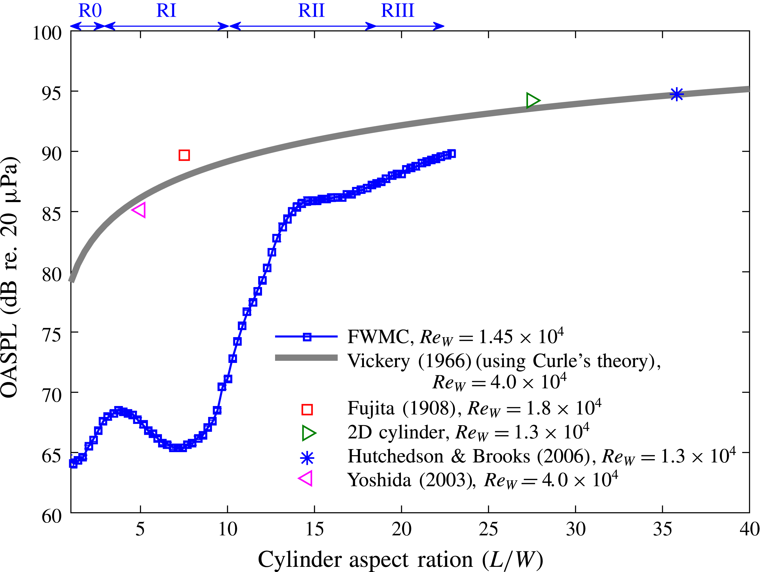
A comparison of OASPLs in dB re.
 $20~\unicode[STIX]{x03BC}\text{Pa}$
for square FWMCs with aspect ratios in the range
 $0.29\leqslant L/W\leqslant 22.9$
. The data are compared with (3.1) using measurements of an infinite square cylinder provided by Vickery (Reference Vickery1966) (
 $s=6$
,
 $St=0.13$
and
 $\overline{C_{l}^{2}}=1.7$
) and experimentally obtained noise data measured by Fujita et al. (Reference Fujita, Sha, Furutani and Suzuki1998), Yoshida, Koike & Fukano (Reference Yoshida, Koike and Fukano2003) and Hutcheson & Brooks (Reference Hutcheson and Brooks2006) for 2D square cylinders of various lengths. The boundaries of the different shedding regimes, R0 to RIII, are shown at the top.

Figure 10 shows the measured overall sound pressure level (OASPL) in dB re.
 $20~\unicode[STIX]{x03BC}\text{Pa}$
against the aspect ratio for
 $0.29\leqslant L/W\leqslant 22.9$
as measured by the single microphone above the FWMC. To estimate the OASPL, the experimental time series data were first digitally bandpass filtered between 0.3 kHz and 16 kHz using a sixth order bandpass Butterworth filter. The OASPL was then estimated as the mean-square pressure of the filtered time series. The statistical random error in the OASPL estimate is
 $\pm 0.4~\text{dB}$
re.
 $20~\unicode[STIX]{x03BC}\text{Pa}$
with 95 % confidence (Bendat & Piersol Reference Bendat and Piersol2010). Figure 10 also compares the experimental results with the theoretical OASPL calculated by (3.1). The theoretical prediction was calculated using an experimentally obtained Strouhal number of
 $St=0.13$
, a correlation factor of
 $s=6$
and a sectional mean-square lift coefficient
 $\overline{C_{l}^{2}}=1.7$
which were acquired from experiments on an infinitely long square cylinder in flow with
 $Re_{W}=4\times 10^{4}$
by Vickery (Reference Vickery1966). Curle’s theory predicts that given constant values of
 $s$
,
 $St$
and
 $\overline{C_{l}^{2}}$
, the OASPL of an infinite cylinder (with end plates if
 $L/W<30$
) will vary linearly with the aspect ratio. Figure 10 also compares (3.1) with experimentally measured OASPLs of several square cylinders fitted with end plates (‘infinitely’ long) with various aspect ratios (ranging from
 $L/W=6$
to
 $L/W=33$
) and Reynolds numbers (ranging from
 $Re_{W}=1.3\times 10^{4}$
to
 $Re_{W}=4\times 10^{4}$
). The data were taken by Fujita et al. (Reference Fujita, Sha, Furutani and Suzuki1998) for an infinite square cylinder with
 $L/W=8$
(with end plates), Hutcheson & Brooks (Reference Hutcheson and Brooks2006) for a 2D square cylinder with
 $L/W=33$
(with end plates), Yoshida et al. (Reference Yoshida, Koike and Fukano2003) for a 2D square cylinder with
 $L/W=6$
(with end plates) and an infinite square cylinder with
 $L/D=27.5$
taken in the AWT (without end plates). The results have been rescaled to a velocity of
 $32~\text{m}~\text{s}^{-1}$
and a cylinder width of
 $W=7~\text{mm}$
using (3.1). The experimentally obtained OASPLs for infinitely long cylinders show good agreement with those predicted by (3.1) using the data of Vickery (Reference Vickery1966). This indicates that the wake dynamics of infinitely long square cylinders is aspect ratio and Reynolds number invariant within the Reynolds number range of
 $1.3\times 10^{4}<Re_{W}<4\times 10^{4}$
and aspect ratio range of
 $6<L/W<33$
.
The variation of the OASPL for the FWMCs with aspect ratio deviates significantly from that predicted by (3.1), in both trend and magnitude. For all aspect ratios, the OASPL is less than that predicted by (3.1). For very low aspect ratios (
 $L/W<2$
), it is expected that regular periodicity in the wake is suppressed through strong downwash (Sumner, Heseltine & Dansereau Reference Sumner, Heseltine and Dansereau2004; Hosseini et al.
Reference Hosseini, Bourgeois and Martinuzzi2013), so a lower OASPL is expected. However, even for
 $L/W\geqslant 2$
, where vortex shedding is present, the measured OASPL is below the predicted value. This highlights the disruptive impact that the junction and the free end have on the vortex shedding characteristics across the span of the FWMC.
As the aspect ratio increases above
 $L/W=15$
, the OASPL approaches the value predicted by (3.1). For example, at
 $L/W=23$
, the difference between the value of (3.1) and the experimental value of the FWMC is only 3 dB. However, for
 $0.29\leqslant L/W\leqslant 22.9$
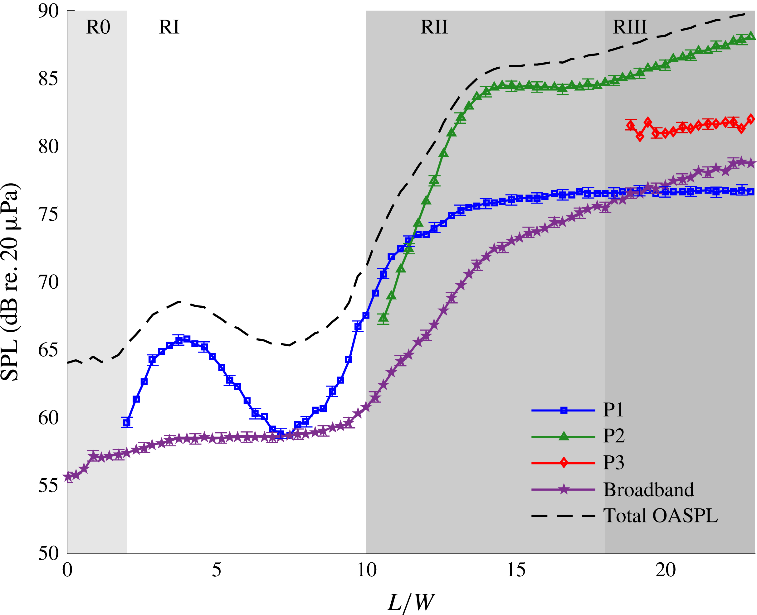
, the variation of the OASPL is not monotonic. At this point, it is convenient to split the variation of the OASPL with the FWMC aspect ratio as a transition through four aspect ratio shedding regimes, called R0–RIII. The aspect ratio ranges over which these regimes are defined are shown in figure 10.
The first regime, known as the ‘very-low-aspect-ratio regime’ or R0, occurs for
 $L/W<2$
. For these low-aspect-ratio cylinders, the noise levels are less than 1 dB above background noise levels. As will be shown, in R0, tonal vortex shedding noise is not detected by the microphone.
The second regime, known herein as the ‘low-aspect-ratio regime’ or RI, occurs for
 $2\leqslant L/W<10$
and is characterised by a local maximum in the OASPL which occurs at
 $L/W\approx 4$
and a local minimum in the OASPL which occurs at
 $L/W\approx 7$
. Similar observations have been made by Moreau & Doolan (Reference Moreau and Doolan2013) on circular FWMCs, where the OASPL was observed to increase at
 $L/D=3.1$
. In this study, it was explained that below
 $L/D=8$
, vortex shedding was suppressed except at
 $L/D=3.1$
, where vortex shedding reappeared. One Aeolian tone is measured throughout this regime, although it is substantially weaker at
 $L/W=7$
than at
 $L/W=4$
(see §§ 3.2.1, 3.2.2 and 3.2.4).
The third regime, known herein as the ‘transitional-aspect-ratio regime’ or RII, occurs for
 $10<L/W<18$
. In this regime, the OASPL experiences a very rapid rate of increase, increasing by 15 dB between
 $L/W=10$
and
 $L/W=14$
. Afterwards, a small plateau occurs between
 $L/W=14$
and
 $L/W=16$
where the OASPL remains constant, after which it begins to rise.
The fourth and final regime, known herein as the ‘high-aspect-ratio regime’ or RIII, occurs for
 $L/W\geqslant 18$
. Here, the OASPL steadily rises from 87 dB at
 $L/W=18$
to 90 dB at
 $L/W=23$
. Between
 $L/W=18$
and
 $L/W=23$
, the rate of increase of the OASPL is much slower than in RII. Nevertheless, this slower rate of increase is still larger than what one would expect for an infinite cylinder and the OASPL is still below that predicted by (3.1). The OASPL will approach that of (3.1) as the aspect ratio is increased towards infinity because the relative influences of the junction and free-end regions become small compared with the mid-span of the cylinder. It is remarkable that end effects can have such a profound impact on the properties of the flow-induced noise from the cylinder even at aspect ratios as high as
 $L/W\approx 20$
. In fact, if the curve for FWMC noise in figure 10 were linearly extrapolated until it intersected the theoretical curve generated by (3.1), it would intersect at approximately
 $L/D=30$
, consistent with the observations of aerodynamic lift and drag made by Fox & West (Reference Fox and West1993) for circular FWMCs.
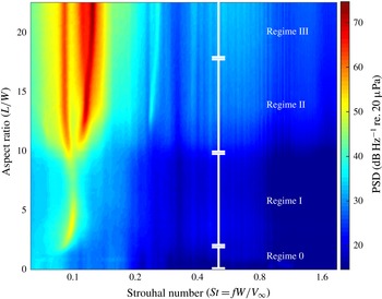
Variation of the acoustic PSD with aspect ratio, expressed in
 $\text{dB}~\text{Hz}^{-1}$
re.
 $20~\unicode[STIX]{x03BC}\text{Pa}$
, for
 $V_{\infty }=32~\text{m}~\text{s}^{-1}$
. The labelled shedding regime boundaries correspond to spectra with 0, 1, 2 and 3 vortex shedding tones respectively.

3.1.2 Acoustic power spectral density
The power spectral density (PSD) of the acoustic signal is used to investigate vortex shedding in more detail. To generate the PSD of the acoustic pressure fluctuations, the same acoustic pressure time records as used to calculate the OASPL were digitally bandpass filtered between 0.3 kHz and 16 kHz using a sixth order bandpass Butterworth filter. The autospectra were then estimated using Welch’s averaged modified periodogram method (Welch Reference Welch1967). The records were divided into
 $B=479$
blocks, each with
 $2^{12}$
data points, giving a frequency resolution of
 $\unicode[STIX]{x0394}f=8~\text{Hz}$
, or
 $\unicode[STIX]{x0394}St=0.002$
. The uncertainty at each narrowband frequency is
 $\pm 0.5~\text{dB}~\text{Hz}^{-1}$
with a 95 % level of confidence (Bendat & Piersol Reference Bendat and Piersol2010).
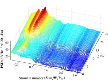
Figure 11 shows the variation of acoustic PSD with aspect ratio for
 $V_{\infty }=32~\text{m}~\text{s}^{-1}$
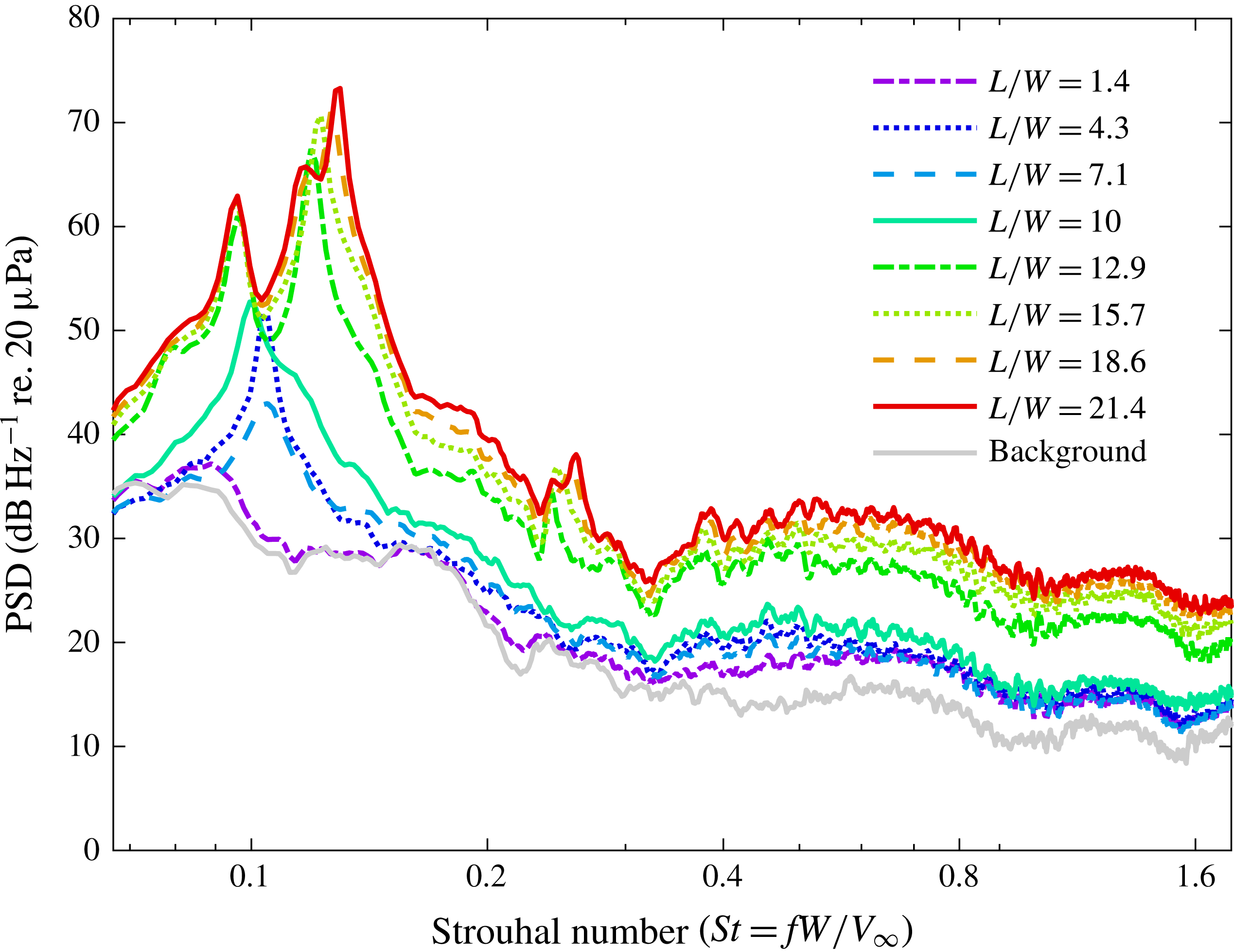
. Figure 12 is a waterfall diagram of the same data, showing the shape of the individual autospectra across all aspect ratios. Finally, figure 13 shows the autospectra for select aspect ratio FWMCs compared with the background level, which is the level obtained with the cylinder removed, but with the mounting plate still attached to the contraction.
Variation of the acoustic PSD with aspect ratio of the FWMC, presented as a waterfall diagram, expressed in
 $\text{dB}~\text{Hz}^{-1}$
re.
 $20~\unicode[STIX]{x03BC}\text{Pa}$
, for
 $V_{\infty }=32~\text{m}~\text{s}^{-1}$
. The colour is proportional to the PSD level.

Narrowband acoustic spectra for selected aspect ratio FWMCs for
 $V_{\infty }=32~\text{m}~\text{s}^{-1}$
. The frequency resolution is
 $\unicode[STIX]{x0394}f=8~\text{Hz}$
or
 $\unicode[STIX]{x0394}St=0.002$
.

Figure 13 shows that in R0 (
 $L/W<2$
), no tonal components are measured and the spectrum for
 $St<0.3$
collapses onto the background spectrum (the noise measured with the plate and no cylinder in place). The absence of any sharp peak near
 $St=0.1$
suggests that regular vortex shedding is either too weak to be detected or is suppressed.
In RI, the acoustic spectrum is characterised by a single Aeolian peak centred at approximately
 $St=0.1$
(see figure 11). Figure 13 shows that the exact frequency of the dominant peak changes as the aspect ratio increases from 2 to 10. An important feature in RI is that the magnitude of the peak at
 $L/W=7.1$
is weaker than that at
 $L/W=4.3$
, which explains the existence of a local minimum in the OASPL at
 $L/W=7.1$
in figure 10.
In RII, the frequency spectrum changes dramatically. A bifurcation occurs at
 $L/W\approx 10$
and two vortex shedding peaks are observed, one at
 $St<0.10$
and one at
 $St>0.10$
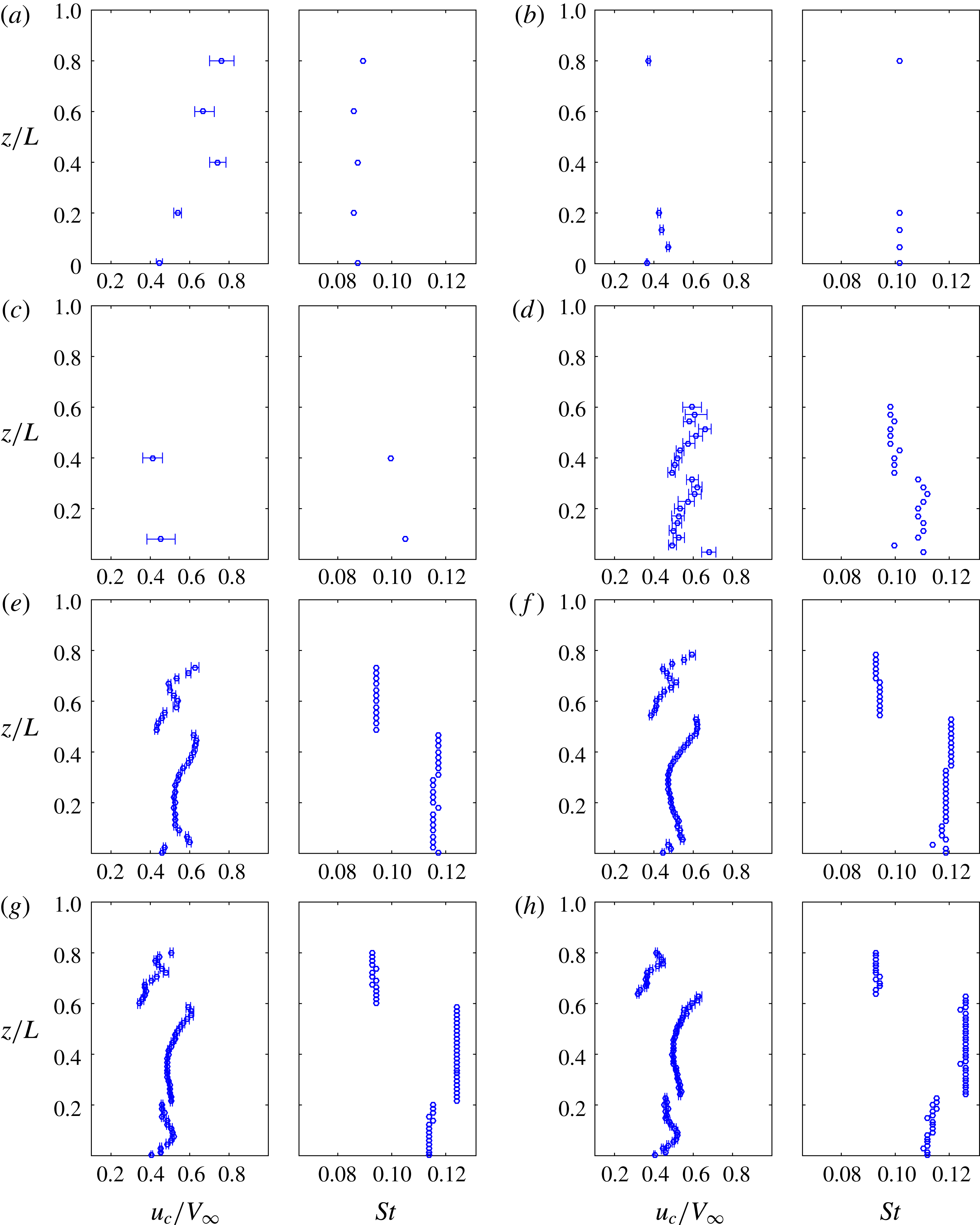
(see figure 11). Moreau & Doolan (Reference Moreau and Doolan2013) showed that these two peaks are caused by two different vortex shedding frequencies occurring along the cylinder axis. The dual peaks are indicative of a cellular shedding mode that sometimes occurs in infinite circular cylinders (Gerich & Eckelmann Reference Gerich and Eckelmann1982) given the right inflow conditions. A cellular shedding mode is where different spanwise portions of the cylinder shed with different frequencies, creating different spanwise ‘cells’ of constant frequency. According to Moreau & Doolan (Reference Moreau and Doolan2013), the lower-frequency peak is associated with a cell of vortex structures towards the free end of the cylinder and the higher-frequency peak with a second cell of vortex structures towards the junction.
In a similar manner to RII, the beginning of RIII is also characterised by a bifurcation that occurs at
 $L/W\approx 18$
at
 $St=0.115$
, creating a third peak between the two previous ones. This peak is difficult to observe in figure 11 due to the colour scheme, but can be clearly seen in figures 12 and 13. These results demonstrate that a triple cellular shedding mode is occurring in the wake of the cylinder. A triple shedding mode has never before been observed in square FWMC flow, probably because all other investigations have focused on aspect ratios
 $L/W<14$
.
3.1.3 Peak frequency
As shown in figure 13, the acoustic spectrum of an FWMC will exhibit up to three main peaks in the acoustic spectrum depending on the aspect ratio. For regime R0, no peaks occur. In RI, only one dominant peak can be identified. This peak is known as ‘P1’ and varies with the aspect ratio within RI. The peak P1 continues to exist into RII and RIII as the lower-frequency peak. In RII, in the range
 $10<L/W<18$
, a second, higher-frequency, peak occurs, referred to as ‘P2’. Finally, for
 $L/W>18$
, a third peak occurs between P1 and P2, known as ‘P3’. Like P1, the frequencies of P2 and P3 also vary with the aspect ratio within their respective regimes.
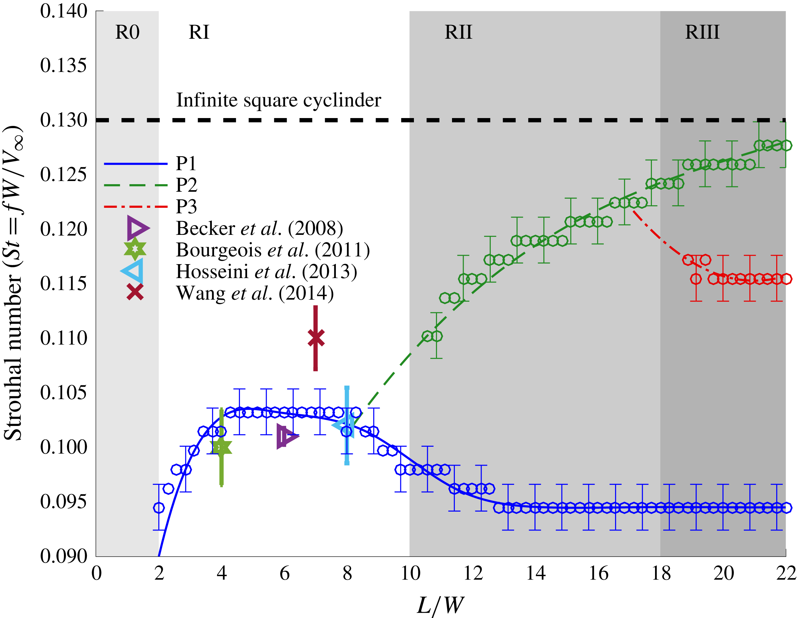
Figure 14 plots the frequency (Strouhal number) of each peak as a function of the aspect ratio. Because of the finite frequency resolution (
 $\unicode[STIX]{x0394}f=8~\text{Hz}$
), the uncertainty in the peak frequency (at 95 % confidence assuming a rectangular distribution) is approximately
 $f_{e}=\pm 2\unicode[STIX]{x0394}f/\sqrt{3}=\pm 9.2~\text{Hz}$
, corresponding to a Strouhal number uncertainty of
 $St_{e}=\pm 0.002$
, shown as error bars in figure 14. Also shown are the measured Strouhal numbers of vortex shedding of various aspect ratio square FWMCs measured in other studies. These measurements include that of Becker et al. (Reference Becker, Hahn, Kaltenbacher and Lerch2008) for an
 $L/W=6$
square FWMC using a far-field microphone and those of Bourgeois et al. (Reference Bourgeois, Sattari and Martinuzzi2011), Hosseini et al. (Reference Hosseini, Bourgeois and Martinuzzi2013) and Wang et al. (Reference Wang, Cao and Zhou2014) for
 $L/W=8$
, 6 and 4 square FWMCs respectively, using hot-wire anemometry.
The variation of the frequency of each peak (P1, P2 and P3) as a function of the FWMC aspect ratio. The data are compared with the vortex shedding peak frequencies of square FWMCs from other studies including Hosseini et al. (Reference Hosseini, Bourgeois and Martinuzzi2013) (
 $L/W=8$
,
 $Re=1.2\times 10^{4}$
and
 $\unicode[STIX]{x1D6FF}/W=0.72$
), Wang et al. (Reference Wang, Cao and Zhou2014) (
 $L/W=7$
,
 $Re=0.93\times 10^{4}$
and
 $\unicode[STIX]{x1D6FF}/W=1.35$
), Becker et al. (Reference Becker, Hahn, Kaltenbacher and Lerch2008) (
 $L/W=6$
,
 $Re=3.8\times 10^{4}$
and
 $\unicode[STIX]{x1D6FF}/W=0.27$
) and Bourgeois et al. (Reference Bourgeois, Sattari and Martinuzzi2011) (
 $L/W=4$
,
 $Re=1.2\times 10^{4}$
and
 $\unicode[STIX]{x1D6FF}/W=0.72$
). The frequency,
 $f$
, is non-dimensionalised as the Strouhal number,
 $St=fW/V_{\infty }$
.

Initially, P1 increases from
 $St=0.09$
and appears to reach a stable value of
 $St=0.102$
in the range
 $4<L/W<8$
. This is the aspect ratio range where most other investigations on square FWMCs have taken place and there is good agreement between the present results and other studies. The exception is the study by Wang et al. (Reference Wang, Cao and Zhou2014), who measured a Strouhal number of
 $St=0.11$
for an
 $L/W=7$
square FWMC in a boundary layer thickness of
 $\unicode[STIX]{x1D6FF}/W=1.35$
and a Reynolds number of
 $Re=0.93\times 10^{4}$
.
In the range
 $7.7<L/W<14$
, the Strouhal number of P1 decreases. At
 $L/W=14$
, the beginning of RIII, the Strouhal number of P1 reaches a constant value of
 $St=0.095$
. At the same time, P2 starts to occur at
 $L/W=10.6$
, the beginning of RII, and the Strouhal number of P2 increases in value towards the two-dimensional value of
 $St=0.13$
as the aspect ratio increases. The peak P3 begins to form at
 $L/W=18$
and by
 $L/W=18.9$
is sufficiently well resolved to be distinct from P2. The Strouhal number of P3 is constant at
 $St=0.115$
.
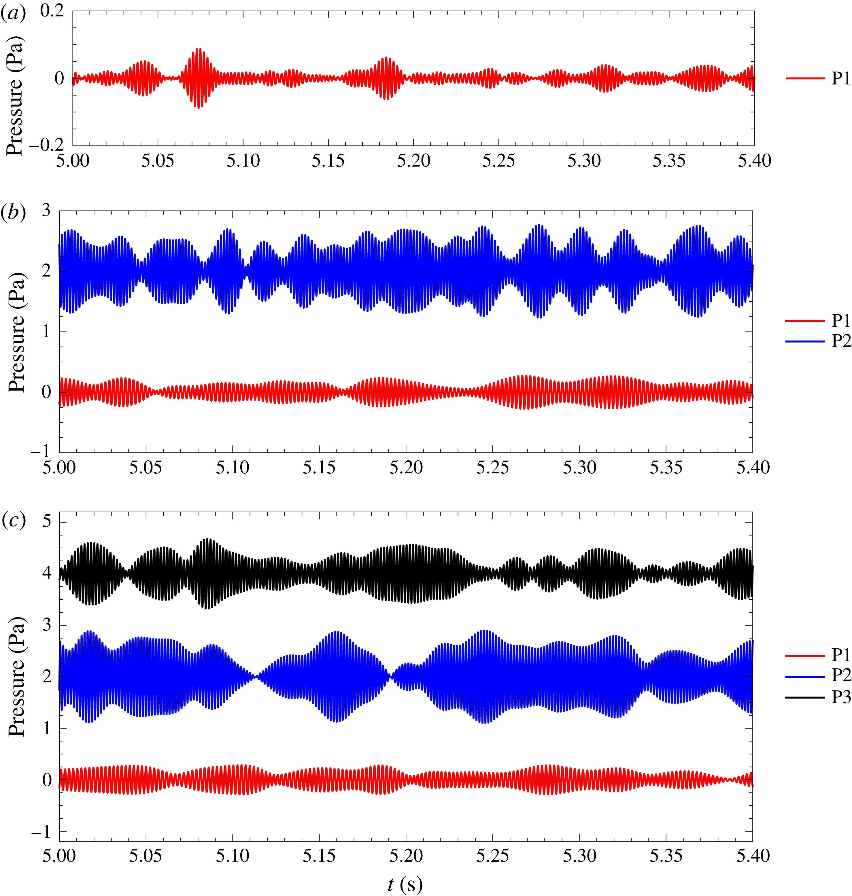
Figure 15 shows the time series of acoustic measurements for FWMCs with three selected aspect ratios of
 $L/W=7.1$
, 15.7 and 21.4 at the peak tonal frequencies. This figure shows a 0.4 s long time series of the measured data that has been filtered using a bandpass Butterworth filter with 80 Hz bandwidth centred on the peak tonal frequencies (P1–P3). The temporal evolution of the acoustic tones can be seen in figure 15. The tonal noise displays random modulation and is observed to occur in short bursts. Time series data indicate that the vortex shedding modes responsible for tonal noise generation occur intermittently and independently.
Time series of acoustic signals for the FWMCs at the peak tonal frequencies: (a)
 $L/W=7.1$
, RI; (b)
 $L/W=15.7$
, RII; (c)
 $L/W=21.4$
, RIII. The time series of the acoustic signals at P2 and P3 have been offset by 2 and 4 Pa respectively.

3.1.4 Peak magnitude
Figure 16 shows the magnitudes of P1–P3 and the broadband component against aspect ratio. The magnitude of an individual peak in the acoustic spectrum is defined as the sound pressure level (SPL) obtained when the acoustic spectrum is integrated in a frequency band arranged symmetrically around the peak frequency. Here, the integration bandwidth was set to 48 Hz (much larger than the half-power bandwidth of each peak). The magnitude of the broadband noise is defined as the level obtained when integrating the acoustic spectrum from
 $St=0.3$
to
 $St=2$
. The uncertainty limits in the magnitude were calculated by integrating the upper and lower limits of the 95 % confidence interval of the acoustic spectrum (Bendat & Piersol Reference Bendat and Piersol2010) and are shown in the figure. The OASPL calculated previously is overlaid for reference.
The variation of the magnitude of each peak (P1, P2 and P3) and the broadband component as a function of the FWMC aspect ratio.

The peak P1 starts to occur at the beginning of RI with a magnitude of approximately 57 dB and rises to a local maximum of 66 dB at
 $L/W=4$
. At
 $L/W=4$
, 54 % of the total OASPL is contained in P2, indicating that at
 $L/W=4$
, P1 is the dominant source of noise. In contrast, at
 $L/W=7.4$
, the magnitude of P1 drops significantly to 58 dB. In fact, the reduction in noise magnitude is so great that the levels become comparable to the broadband noise levels. At
 $L/W=7.4$
, both the broadband component and P1 contribute approximately 20 % to the total OASPL, with the remaining 60 % contributed by other low-frequency sources in the spectrum. The OASPL correspondingly decreases to a level only slightly higher than the background level (the level obtained at
 $L/W=0$
in figure 10). Throughout RI, the broadband noise levels stay approximately constant at
 ${\approx}58~\text{dB}$
, irrespective of the aspect ratio.
Towards the end of RI, there is a rapid increase in the magnitude of P1. From
 $L/W=7.4$
to 14, the magnitude of P1 increases from 58 dB to 75 dB. This increase continues into the beginning of RII, after which the rate of increase gradually slows. Beyond
 $L/W=14$
(towards the end of RII and into RIII), the magnitude of P1 remains constant at 75 dB.
The beginning of RII also marks the onset of P2. The magnitude of P2 rapidly increases as soon as P2 forms, increasing from 67 dB to 84 dB from
 $L/W=10.6$
to 14. The rapid increase of both P1 and P2 at the beginning and end of RII respectively causes a rapid rise in the OASPL throughout RII. By the end of RII, P2 overtakes P1 as the dominant source of noise, contributing 70 % of the OASPL. Unlike P1, the rate of increase in the magnitude of P2 stops abruptly at
 $L/W=14$
to create a small plateau. After maintaining a constant level over most of RI, the broadband component increases from
 $L/W=10$
to 23. However, like P2, this increase is most rapid in RII and, at
 $L/W=14$
, the rate of change of the magnitude of the broadband noise decreases. Based on these observations, it is concluded that
 $L/W=14$
marks a significant change in the noise producing mechanisms of FWMCs and that the flow structures that produce P2 (and evidently the broadband noise component) are affected by this change. Conversely, the structures that generate P1 are not affected by this change.
From
 $L/W=14$
to 18, the magnitude of P2 stabilises at 84.5 dB, which causes the OASPL to maintain a constant level. During this, P2 contributes increasingly less noise to the OASPL, decreasing from 73 % at
 $L/W=14\,\%$
to 60 % at
 $L/W=18$
. When P3 starts to form at
 $L/W=18$
(the boundary between RII and RIII), the magnitude of P2 begins to rise again to a final value of 88 dB and its contribution increases from 60 % at
 $L/W=18\,\%$
to 66 % at
 $L/W=23$
. From an aspect ratio of
 $L/W=18$
, the magnitude of P3 remains constant at 81 dB and contributes increasingly less to the OASPL, starting from 24 % at
 $L/W=18.9\,\%$
to 16.3 % at
 $L/W=23$
. Interestingly, when P3 is formed, the magnitude of the broadband component slightly exceeds that of P1. By
 $L/W=23$
, the broadband component contributes approximately 7.7 % of the OASPL, while P1 contributes only 4 %.
3.2 Wake velocity measurements
3.2.1 Mean velocity
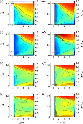
Figure 17 shows colourmaps of normalised mean velocity contours in the wake of the FMWCs. The abscissa axis has been normalised by the span of each cylinder so that
 $z/L=1$
is the free end and
 $z/L=0$
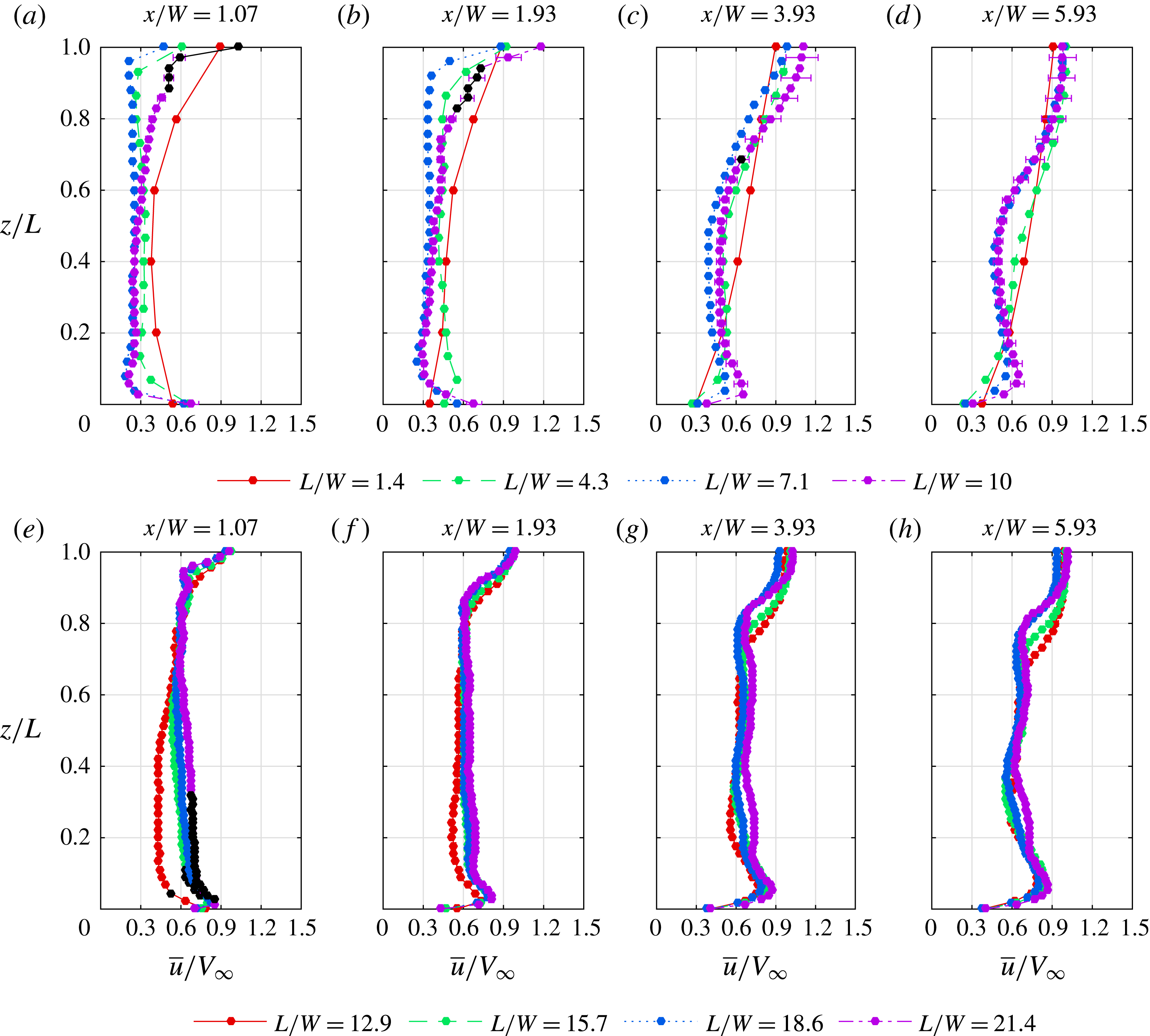
is the junction of the cylinder. The relative height of the boundary layer for each aspect ratio is indicated by a dashed line. Figure 18 directly compares the mean velocity between aspect ratios at various downstream stations. The 95 % confidence levels shown in figure 18 were calculated by taking the square and the sum of the variances of the statistical and experimental uncertainties (Bendat & Piersol Reference Bendat and Piersol2010). The uncertainty at
 $L/W=10$
is larger than other aspect ratio FWMCs because of the large hot-wire drift error during the measurement. It should also be noted that the mean streamwise velocity may be overpredicted by as much as 5 % in regions of turbulence intensity
 $T.I.>0.3$
. In these results, no correction is applied for high-turbulence effects, but spatial regions of
 $T.I.>0.3$
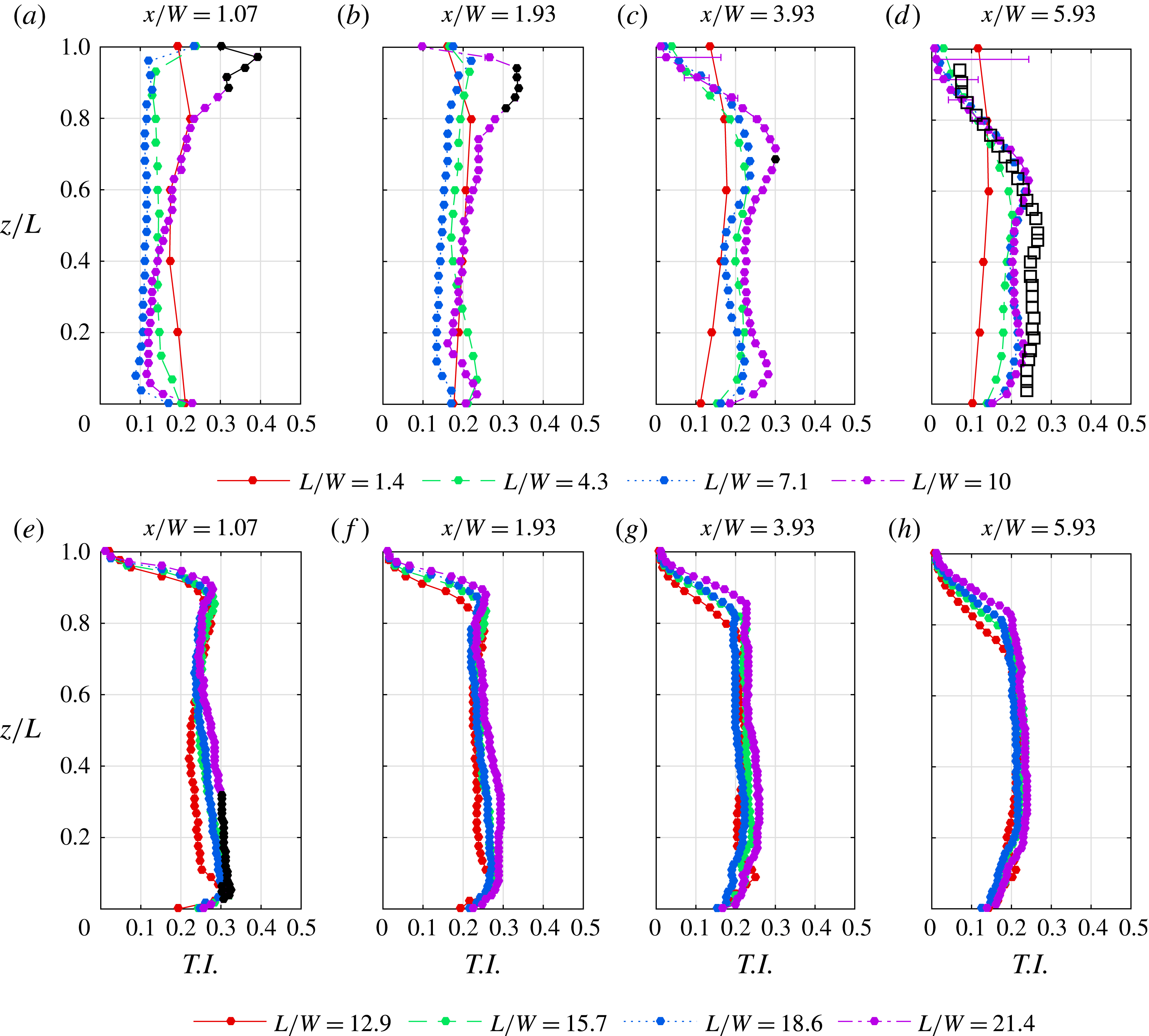
are shaded with cross-hatching in figure 17 and also shown in black in figure 18.
Colourmaps showing the mean velocity contours in the wake of eight different aspect ratio FMWCs: (a)
 $L/W=1.4$
, R0; (b)
 $L/W=4.3$
, RI; (c)
 $L/W=7.1$
, RI; (d)
 $L/W=10$
, RII; (e)
 $L/W=12.9$
, RII; (f)
 $L/W=15.7$
, RII; (g)
 $L/W=18.6$
, RIII; (h)
 $L/W=21.4$
, RIII. The mean velocity is normalised by the free-stream velocity,
 $V_{\infty }=32~\text{m}~\text{s}^{-1}$
, while the ordinate axis has been normalised by the height of each cylinder so that
 $z/L=1$
is the free end of the cylinder. The plane of the hot-wire measurements was
 $y/W=0.6$
. The relative height of the boundary layer for each aspect ratio is indicated by a dashed line.

A salient feature of each map in figure 17 is the size of the region of higher-velocity fluid in the upper right corner. The region is indicative of velocity recovery in the wake, and is related to the descending shear layer over the free end. The pressure difference between the free stream and the cylinder base accelerates high-velocity irrotational fluid from the free stream over the free end and transports it into the wake core, a process known as ‘downwash’ (Rostamy et al. Reference Rostamy, Sumner, Bergstrom and Bugg2012). (‘Base’ refers to the leeward wall of the cylinder, not the junction of the cylinder.) The stronger the downwash is, the more rapid the velocity recovery is and the deeper the free stream descends into the wake. According to Wang et al. (Reference Wang, Zhou, Chan and Lam2006) and Bourgeois et al. (Reference Bourgeois, Sattari and Martinuzzi2011), the presence of downwash implies the presence of a pair of streamwise ‘free-end’ vortices, whose sense of rotation acts to draw fluid from the free stream and push it down in the wake.
The spanwise mean velocity profiles at various downstream locations in the wake: (a)
 $1.4<L/W<10$
; (b)
 $12.9<L/W<21.4$
.

At
 $L/W=1.4$
in figure 17(a), the shear layer descends across the entire cylinder span. The velocity, however, never recovers to the free-stream value. This is due to the relatively high height of the boundary layer compared with the span of the cylinder (
 $\unicode[STIX]{x1D6FF}/L\approx 0.9$
). Because the boundary layer itself contains low-velocity fluid, the imminent acceleration of this fluid over the free end into the wake still results in a streamwise velocity lower than the free stream. Accordingly, as the aspect ratio increases to
 $L/W=4.3$
and 7.1 in figures 17(b) and 17(c), the relative height of the boundary layer reduces to
 $\unicode[STIX]{x1D6FF}/L\approx 0.3$
and 0.2 respectively, and the velocity recovers to the free-stream value. At
 $L/W=10$
, figure 18(d) shows that there is a region at
 $x/W=3$
and
 $z/L=1$
where the velocity is 20 % greater than the free stream. While this may indicate that there is enhanced acceleration around the free end, implying that the base pressure at the free end for
 $L/W=10$
is higher than
 $L/W<10$
, the measurements were taken in regions of high turbulence intensity and could be an artificial inflation of the mean velocity. At
 $L/W\geqslant 12.9$
, the maximum velocity recovery returns to the free-stream value (see figure 17
e–h).
As
 $L/W$
increases from 12.9 to 21.4, the extent that the free stream penetrates into the wake approaches aspect ratio independence. The results suggest that at
 $L/W\geqslant 12.9$
, the wake dynamics of the free end decouples from the wake dynamics of the mid-span and the junction.
A second important feature of the mean velocity maps in figure 17 is the injection of high-speed fluid near the junction of the cylinder, starting at
 $x/W\approx 2$
. According to Bourgeois (Reference Bourgeois2012), high-speed fluid near the junction is an indication of the presence of ‘upwash’, where high-speed fluid from the free stream is entrained into the wake and forced, in a spanwise direction, into the reverse flow region. With this upwash, a significant amount of streamwise flow is present, due to the entrainment of free-stream fluid. Similarly to downwash, Hosseini et al. (Reference Hosseini, Bourgeois and Martinuzzi2013) has related upwash to the presence of streamwise junction vortices.
From figure 17(a), it appears that no upwash exists at
 $L/W=1.4$
. As the aspect ratio increases to
 $L/W=21.4$
in figure 17(h), the magnitude of the streamwise velocity at the junction progressively increases. A jet-like injection forms at
 $x/W\approx 2$
, which rises, in the spanwise direction, off the plate as the measurement position moves downstream. A local maximum in the streamwise velocity is measured for
 $L/W\geqslant 7.1$
at
 $z/L\approx 0.1$
and
 $x/W=6$
, as demonstrated in figure 18.
For
 $L/W\leqslant 4.3$
, no local maximum in the junction mean velocity exists (see figure 18); hence, upwash is weak or not existent for
 $L/W<4.3$
. For
 $7.1\leqslant L/W\leqslant 15.7$
, there is a rapid rise in the maximum velocity in the junction region from 55 % of the free-stream value to approximately 85 % of the free-stream value, after which the upwash becomes independent of the aspect ratio. Upwash is still weak at
 $L/W=7.1$
, but strengthens rapidly as
 $L/W$
approaches 12.9. By the time the FWMC reaches
 $L/W=15.7$
, upwash is strong, but invariant with aspect ratio.
3.2.2 Turbulence intensity
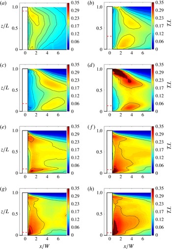
Figure 19 shows colourmaps of the streamwise turbulence intensity contours in the wake of the FWMCs. Here, the streamwise turbulence intensity is denoted
 $T.I.=\unicode[STIX]{x1D70E}_{u}/V_{\infty }$
, and is calculated as the standard deviation of the velocity of the signal normalised by the free-stream value. Similarly to figure 17, the abscissa axis has been normalised by the span of each FWMC so that
 $z/L=1$
is the free end. The height of the boundary layer relative to the FWMC span for each aspect ratio is indicated by a dashed red line. Figure 20 compares the turbulence intensity between aspect ratios at various downstream stations. Figure 20(a) also compares the turbulence intensity results with similar results from Wang et al. (Reference Wang, Zhou, Chan and Lam2006) at
 $x/W=6$
for an FWMC with
 $L/W=6$
. The uncertainty bounds of the turbulence intensity were calculated by taking the sum of the square of the experimental uncertainty and statistical uncertainty (Bendat & Piersol Reference Bendat and Piersol2010). The large error for the measurements at
 $L/W=10$
is a result of the relatively large hot-wire drift error during these measurements. Once again, spatial regions of
 $T.I.>0.3$
are shaded with cross-hatching in figure 19 and also shown in black in figure 20. Unlike mean velocity measurements, turbulence intensity measurements are relatively insensitive to transverse turbulence, and the error is estimated to be less than 2 % for
 $T.I.<0.3$
.
Colourmaps showing the turbulence intensity contours in the wake of eight different aspect ratio FWMCs: (a)
 $L/W=1.4$
, R0; (b)
 $L/W=4.3$
, RI; (c)
 $L/W=7.1$
, RI; (d)
 $L/W=10$
, RII; (e)
 $L/W=12.9$
, RII; (f)
 $L/W=15.7$
, RII; (g)
 $L/W=18.6$
, RIII; (h)
 $L/W=21.4$
, RIII. The turbulence intensity is denoted
 $T.I.=\unicode[STIX]{x1D70E}_{u}/V_{\infty }$
, calculated as the standard deviation of the velocity of the signal normalised by the free-stream value. The ordinate axis has been normalised by the span of each cylinder so that
 $z/L=1$
is the free end of the cylinder. The plane of the hot-wire measurements was
 $y/W=0.6$
. The relative height of the boundary layer for each aspect ratio is indicated by a dashed line.

Spanwise profiles of the turbulence intensity at various downstream locations in the wake: (a)
 $L/W=1.4\leqslant L/W\leqslant 10$
; (b)
 $12.9<L/W\leqslant 21.4$
. The results are also compared with similar results from Wang et al. (Reference Wang, Zhou, Chan and Lam2006) at
 $x/W=6$
for an
 $L/W=6$
FWMC (square symbols).

Figure 19 shows that for
 $L/W=4.3$
, 7.1 and 10, there are two prominent concentrations of turbulence intensity, one near the free end and one near the junction. For
 $L/W=1.4$
, only one concentration exists. The results are qualitatively similar to the particle image velocimetry measurements presented by Wang & Zhou (Reference Wang and Zhou2009) for
 $L/W=3$
, 5 and 7 square FWMCs in a similar boundary layer height of
 $\unicode[STIX]{x1D6FF}/W=1.35$
at a slightly lower Reynolds number of
 $Re_{W}=0.93\times 10^{4}$
. In that study, the turbulence intensity field of the
 $L/W=3$
cylinder wake displayed only one maximum near the free end, while the turbulence intensity fields of the
 $L/W=5$
and 7 wakes displayed two maxima. According to Wang & Zhou (Reference Wang and Zhou2009), the presence of two maxima in the turbulence field is caused by streamwise junction and free-end vortices, respectively. A cylinder with
 $L/W=3$
was found (using streamwise vorticity measurements) to have a dipole vortex topology, where a pair of counter-rotating vortices were observed near the free end. On the other hand, cylinders with
 $L/W=5$
and 7 were found to have quadrupole wake topologies, where an additional pair of counter-rotating vortices were found near the junction.
Bourgeois (Reference Bourgeois2012) explained that a dipole wake is the result of ‘half-loop’ shedding, where opposite signed vortices are connected by vortex filaments formed in the separating shear layer over the free end of the cylinder. These filaments are ‘bent’ upstream due to Biot–Savart induction and consequently project a pair of counter-rotating streamwise vortices in the cross-stream plane near the free end. Similarly, Bourgeois (Reference Bourgeois2012) found that a quadrupole wake is the result of ‘full-loop’ shedding, where vortex filaments are also rotated in the upstream direction at the junction due to interaction with the horseshoe vortex. In contrast to the findings of Wang & Zhou (Reference Wang and Zhou2009), Bourgeois (Reference Bourgeois2012) found that the T.I. field will still exhibit two maxima (one at the free end and one at the junction) regardless of whether half- or full-loop shedding occurs, the only difference being that full-loop shedding tends to shift the concentration of turbulence intensity at the junction much closer to the FWMC base when compared with half-loop shedding. Consequently, the present streamwise turbulence intensity maps do not allow for the direct identification of dipole or quadrupole wakes. Hence, there is ambiguity in whether the vortex topologies of
 $L/W=1.4$
–10 are either quadrupole or dipole.
It has been inferred by Bourgeois (Reference Bourgeois2012) that the wake of the
 $L/W=6$
FWMC used by Wang et al. (Reference Wang, Zhou, Chan and Lam2006) immersed in a boundary layer thickness of
 $\unicode[STIX]{x1D6FF}/W=1$
had a quadrupole style wake because of the presence of upwash at the junction. In the present results, no appreciable upwash flow has been measured (or inferred from the mean velocity maps) until
 $L/W=10$
. Therefore, while the present results do not allow for the direct identification of the wake topology, it is likely that FWMCs with
 $L/W<10$
have dipole wakes. Ogunremi & Sumner (Reference Ogunremi and Sumner2015) found that square FWMCs of
 $3\leqslant L/W\leqslant 9$
in a boundary layer of height
 $\unicode[STIX]{x1D6FF}/W=1.5$
had dipole wakes, confirming that the boundary layer must be greater than
 $\unicode[STIX]{x1D6FF}/W=1.5$
for a quadrupole wake to be induced. Hassan, Bourgeois & Martinuzzi (Reference Hassan, Bourgeois and Martinuzzi2015) have also demonstrated that the vortex legs shed off FWMCs with
 $L/W=4$
immersed in a boundary layer thickness of
 $\unicode[STIX]{x1D6FF}/W=1.3$
have less severe wake retraction than that of a quadrupole style wake. One possibility raised by Hassan et al. (Reference Hassan, Bourgeois and Martinuzzi2015) is that their FWMC was in a ‘transitional’ state between quadrupole and dipole vortex topologies.
Unlike their lower-aspect-ratio counterparts, cylinders in RII and RIII (
 $L/W>10$
) do not have well established vortex flow topologies. It is unclear whether these FWMCs have quadrupole or dipole wakes or another alternative. Figure 19(e–h) shows that as the aspect ratio increases above
 $L/W=10$
, the two turbulence intensity concentrations retreat towards the free end and junction respectively, so that they lie at
 $x/W\approx 1$
. The turbulence intensity at the mid-span (
 $z/L=0.5$
) also generally increases with aspect ratio. The high degree of streamwise turbulence intensity near the free-end and junction regions (see figure 20) for these high-aspect-ratio cylinders indicates that strong free-end and junction vortices are present, consistent with a quadrupole style full-loop shedding wake. Section 3.1 has shown, however, that multiple Aeolian like tones exist for these high-aspect-ratio FWMCs, corresponding to a spanwise cellular vortex structure, where different spanwise regions of the cylinder shed with different frequencies. A cellular variation in vortex shedding frequency across the span implies that multiple independent vortex structures form across the FWMC span. Therefore, it is unlikely that conventional full-loop quadrupole or half-loop dipole wake structures, like those described by Wang & Zhou (Reference Wang and Zhou2009) and Bourgeois et al. (Reference Bourgeois, Sattari and Martinuzzi2011), exist at these high aspect ratios.
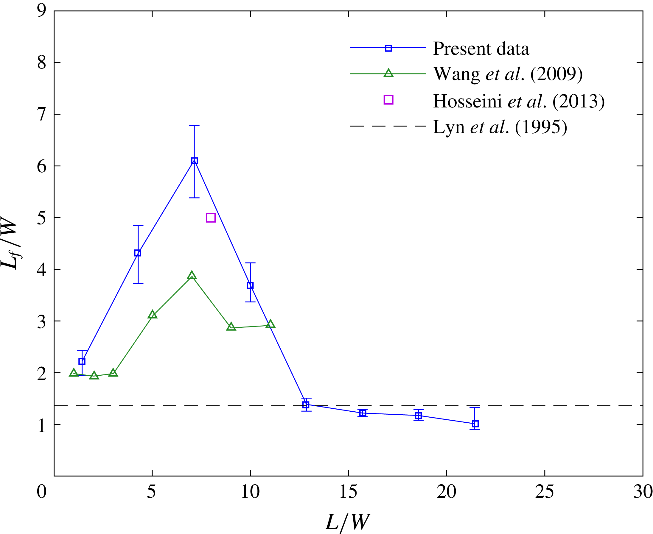
A flow quantity that is commonly used to characterise the wake of an infinite cylinder is the formation length (Williamson Reference Williamson1996). The formation length is defined as the point where the streamwise velocity fluctuations on the wake centreline first reach a local maximum. The physical relevance of the formation length of an infinite cylinder is discussed by Gerrard (Reference Gerrard1966) and Unal & Rockwell (Reference Unal and Rockwell1988); it is essentially the point downstream of the cylinder where fluid from outside the wake first crosses the centreline of the cylinder on average. For an infinite cylinder, the length of the formation region is indicative of the strength of vortex shedding; the shorter the formation length is, the higher the Reynolds stress production is and the stronger the vortex shedding is.
Figure 21 plots the location of the maximum of the turbulence intensity at mid-span, a measure of the formation length,
 $L_{f}$
, for different aspect ratio cylinders. These measurements are also compared with similar measurements made by Wang & Zhou (Reference Wang and Zhou2009) (
 $1\leqslant L/W\leqslant 11$
) and Hosseini et al. (Reference Hosseini, Bourgeois and Martinuzzi2013) (
 $L/W=8$
) for square FWMCs and Lyn et al. (Reference Lyn, Einav, Rod and Park1995) for an infinite cylinder.
The variation of the wake formation length,
 $L_{f}/W$
, at the mid-span of the FWMC, with aspect ratio. The results are compared with the data of Wang & Zhou (Reference Wang and Zhou2009) and Hosseini et al. (Reference Hosseini, Bourgeois and Martinuzzi2013) for square FWMCs and Lyn et al. (Reference Lyn, Einav, Rod and Park1995) for an infinite cylinder.

Figure 21 shows that the formation length increases rapidly from approximately
 $L_{f}/W=2$
at
 $L/W=1.4$
to a maximum of
 $L_{f}/W=6$
at
 $L/W=7.1$
, greater than that expected for an infinitely long cylinder found by Lyn et al. (Reference Lyn, Einav, Rod and Park1995). For higher aspect ratios, the formation length becomes similar to that for an infinite cylinder as the flow at the FWMC mid-span becomes free from the influence of the free end and junction.
The most important observation in these results is that the elongation of the formation length at
 $L/W=7$
is coincident with the reduction in the magnitude of P1 (and the OASPL) at
 $L/W=7$
(see figure 16). The turbulence intensity results presented here indicate that the strength of the vortices at
 $L/W=7$
is much less than for those of higher or lower aspect ratio.
3.2.3 Spectral maps
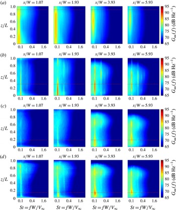
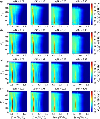
Figures 22 and 23 show spectral maps of the PSDs of the velocity fluctuations, denoted
 $G_{uu}(f)$
, at various downstream positions in the wake for each FWMC. In these maps, the abscissa axis is the Strouhal number of the velocity fluctuations, the ordinate axis is the normalised span of the cylinder and the colour denotes the PSD of the velocity fluctuations in
 $\text{dB}~\text{Hz}^{-1}$
re.
 $20~\unicode[STIX]{x03BC}\text{m}~\text{s}^{-1}$
. The PSDs were estimated using Welch’s averaged modified periodogram method (herein referred to ‘Welch’s method’) (Welch Reference Welch1967) by dividing each time record into
 $B=240$
overlapping blocks of
 $2^{12}$
data points. This gave a frequency resolution of
 $\unicode[STIX]{x0394}f=8~\text{Hz}$
and a spectral density estimate (based on the statistical uncertainty) with a 95 % confidence of
 $\pm 0.6~\text{dB}~\text{Hz}^{-1}$
at each narrowband frequency.
Spectral maps of the streamwise velocity fluctuations,
 $G_{uu}(f)$
, at various downstream stations: (a)
 $L/W=1.4$
, R0; (b)
 $L/W=4.3$
, RI; (c)
 $L/W=7.1$
, RI; (d)
 $L/W=10$
, RII. The values are expressed in
 $\text{dB}~\text{Hz}^{-1}$
re.
 $20~\unicode[STIX]{x03BC}\text{m}~\text{s}^{-1}$
.

Spectral maps of the streamwise velocity fluctuations,
 $G_{uu}(f)$
, at various downstream stations: (a)
 $L/W=12.9$
, RII; (b)
 $L/W=15.7$
, RII; (c)
 $L/W=18.6$
, RIII; (d)
 $L/W=21.4$
, RIII. The values are expressed in
 $\text{dB}~\text{Hz}^{-1}$
re.
 $20~\unicode[STIX]{x03BC}\text{m}~\text{s}^{-1}$
.

The velocity spectral maps at
 $L/W=1.4$
in figure 22(a) show strong fluctuations at
 $St\approx 0.09$
. This indicates that a periodic signal is occurring in the wake of the cylinder, despite the fact that no Aeolian tone is detected. At
 $x/W=1.07$
in figure 22(a), the fluctuations are strongest near the junction region. Moving downstream, the strength of the velocity fluctuations decays, but decays more rapidly at the junction region. Eventually, at
 $x/W=5.93$
, the peak velocity fluctuations occur at
 $z/L=0.7$
.
The wakes shown in figure 22(b–d) for
 $L/W=4.3$
, 7.1 and 10 respectively have different characteristics compared with those of figure 22(a). All three wakes display strong wake periodicity at
 $St\approx 0.1$
. However, unlike figure 22(a), strong velocity fluctuations are not measured close to the cylinder at
 $x/W=1.07$
. Instead, the peak velocity fluctuations occur at
 $x/W\geqslant 2$
. This is consistent with the observation that the formation length is elongated.
Another characteristic is that the highest-magnitude fluctuations first form at the junction region of the cylinder. For example, for
 $L/W=4.3$
at
 $x/W=1.93$
in figure 22(b), the strongest velocity fluctuations are localised entirely within the boundary layer. These observations are consistent with the investigation of Casalino & Jacob (Reference Casalino and Jacob2003), who observed that a cylinder will experience enhanced vortex shedding near an end plate because the end plate prevents spanwise velocity fluctuations from disrupting the wake in that region, thereby promoting two-dimensional flow.
In fact, the wakes appear to be split into two regions, namely a region of strong velocity fluctuations at
 $St=0.1$
near the junction, as discussed previously, and a secondary region of weaker velocity fluctuations, also at
 $St=0.1$
, localised near the free end. These two regions correspond to the two peaks found in the turbulence intensity maps, thus confirming that the peaks in the turbulence intensity are generated by the passage of periodically shed vortices. As demonstrated in the turbulence intensity maps, the spatial separation between the tip and junction fluctuations decreases further downstream. At
 $x/W\approx 6$
, the two peaks merge to form a single ‘cell’ of vortex shedding.
As the aspect ratio increases towards higher values as in figure 23, the wake is dominated by stronger vortex shedding and multi-cellular wake structures. At
 $L/W=12.9$
in figure 23(a), two vortex shedding peaks are observed: a lower frequency peak towards the free end of the cylinder beginning from
 $z/L=0.4$
to 1 and a higher frequency peak at the junction region starting from
 $z/L=0$
to 0.4. The magnitude of the velocity fluctuations at the free-end cell decays downstream at a much faster rate than that associated with the higher-frequency peak at the junction. The same phenomenon is observed for
 $L/W=15.7$
. However, as the aspect ratio increases, the starting point of the free-end cell moves towards the free end of the cylinder, so the total length of the free-end cell remains constant. At
 $L/W=21.4$
, a third cell of vortex shedding is observed at the junction region, which extends from
 $z/L=0$
through the boundary layer to
 $z/L=0.2$
. The frequency of this cell lies between those of the first and second cells. Similarly to the free-end cell, the velocity fluctuations associated with this cell decay downstream at a more rapid rate than the mid-span cell.
3.2.4 Phase maps
Kawamura et al. (Reference Kawamura, Hiwada, Hibino, Mabuchi and Kumada1984), Wang & Zhou (Reference Wang and Zhou2009), Bourgeois, Sattari & Martinuzzi (Reference Bourgeois, Sattari and Martinuzzi2010) and Hosseini et al. (Reference Hosseini, Bourgeois and Martinuzzi2013) used dual hot-wires placed either side of square and circular FWMCs to understand the spatial evolution of the vortices under the action of upwash and downwash. In these studies, an upstream curvature of the vortex filaments was visualised by comparing the average phase between each of the hot-wire signals as one hot-wire was traversed along the span. Here, we educe the orientation of the vortex filaments using a similar technique, but with the reference signal being the acoustic pressure measured with a microphone. A similar analysis was performed by Becker et al. (Reference Becker, Hahn, Kaltenbacher and Lerch2008) but in a cross-stream plane, rather than a plane that was aligned with the free-stream velocity and the cylinder span. The visualisation technique is based on the fact that the location of the microphone is fixed, so the microphone signal serves as a reference signal with fixed statistical properties. Therefore, if at a certain position, the velocity signal has a certain phase difference with the acoustic pressure, and at another position, a similar phase difference is measured, then the two points can be thought of as being in phase. As explained by Bourgeois et al. (Reference Bourgeois, Sattari and Martinuzzi2010), the inherent assumption with this visualisation technique is that the fluctuating velocity at a single point is governed primarily by the nearest vortex, with the effect of other vortices in the flow field being negated. As such, isocontours of constant phase will be aligned with the vortex filaments in the flow.
Figures 24–26 are colourmaps showing the positions in the FWMC wake with similar phase between the velocity fluctuations (measured by the traversing wake hot-wire at
 $y/W=0.6$
) and acoustic pressure fluctuations (measured by the single microphone 0.5 m directly above the cylinder) at the frequency for which each peak was determined. That is, the positions of equal phase at the frequencies where P1, P2 and P3 are mapped in figures 24–26, respectively. To generate these figures, the time-averaged phase at a particular frequency was calculated according to (Bendat & Piersol Reference Bendat and Piersol2010)
 $$\begin{eqnarray}\hat{\unicode[STIX]{x1D719}}_{xy}(f)=\tan ^{-1}\frac{\text{Im}({\hat{G}}_{xy}(f))}{\text{Re}({\hat{G}}_{xy}(f))}.\end{eqnarray}$$
The absolute value of the phase,
 $|\unicode[STIX]{x1D719}(f_{p})|$
, where
 $f_{p}$
is the peak frequency, was taken to avoid sharp discontinuities in the map due to the ambiguity at the
 $-\unicode[STIX]{x03C0}$
to
 $\unicode[STIX]{x03C0}$
boundary. For visual clarity, the colouring of each map is restricted to only show phase from
 $0.5\unicode[STIX]{x03C0}$
to
 $\unicode[STIX]{x03C0}$
.
The spatial distribution of phase,
 $|\unicode[STIX]{x1D719}_{xy}(f_{p1})|$
, at the frequency where P1 occurs: (a)
 $L/W=1.4$
, R0; (b)
 $L/W=4.3$
, RI; (c)
 $L/W=7.1$
, RI; (d)
 $L/W=10$
, RII; (e)
 $L/W=12.9$
, RII; (f)
 $L/W=15.7$
, RII; (g)
 $L/W=18.6$
, RIII; (h)
 $L/W=21.4$
, RIII. The colourmaps are restricted to only show
 $|\unicode[STIX]{x1D719}_{xy}(f_{p1})|=\unicode[STIX]{x03C0}/2$
to
 $\unicode[STIX]{x03C0}$
. The contour levels denote those parts of the in-phase structures that are coherent with the acoustic pressure measured with the microphone.

The spatial distribution of phase,
 $|\unicode[STIX]{x1D719}_{xy}(f_{p2})|$
, at the frequency where P2 occurs: (a)
 $L/W=12.9$
, RII; (b)
 $L/W=15.7$
, RII; (c)
 $L/W=18.6$
, RIII; (d)
 $L/W=21.4$
, RIII. The colourmaps are restricted to only show
 $|\unicode[STIX]{x1D719}_{xy}(f_{p2})|=\unicode[STIX]{x03C0}/2$
to
 $\unicode[STIX]{x03C0}$
. The contour levels denote those parts of the in-phase structures that are coherent with the acoustic pressure measured with the microphone.

The spatial distribution of phase,
 $|\unicode[STIX]{x1D719}_{xy}(f_{p3})|$
, at the frequency where P3 occurs for
 $L/W=21.4$
. The colourmap is restricted to only show
 $|\unicode[STIX]{x1D719}_{xy}(f_{p3})|=\unicode[STIX]{x03C0}/2$
to
 $\unicode[STIX]{x03C0}$
. The contour levels denote those parts of the in-phase structures that are coherent with the acoustic pressure measured with the microphone.

Conceptual sketch of the vortex structures that generate P1: (a)
 $L/W=1.4$
, R0; (b)
 $L/W=4.3$
and 7.1, RI; (c)
 $L/W=10$
, RII; (d)
 $L/W\geqslant 12.9$
, RII and RIII.

Like coherence estimates, the error in the phase angle estimate varies with the coherence level at the measurement point. The 95 % confidence intervals in the phase angle estimates using (3.3) were found to be between
 $\pm 0.01\unicode[STIX]{x03C0}$
radian and
 $\pm 0.09\unicode[STIX]{x03C0}$
radian.
To help to visualise the vortex structures, black contours have been added to represent the distribution of the in-phase structures that are coherent with the microphone. This is calculated by multiplying the absolute value of the phase at each point in space by the value of the coherence between the microphone and the hot-wire at the same point, and scaling the result so that 0 indicates no coherence and 1 indicates full coherence. In this manner, those parts of the vortex structures that are noise producing are shown by the contours. Moreover, figures 27–29 show conceptual sketches of the vortex structures responsible for P1–P3 based on interpretation of the phase maps in figures 24–26.
The maps for P1 (figure 24) show a distinct transition of the noise producing structures moving from cylinders in R0 (
 $L/W<2$
), through RI (
 $2<L/W<10$
) and finally to RII (
 $10<L/W<18$
) and RIII (
 $L/W>18$
). At
 $L/W=1.4$
in figure 24(a) (the only cylinder in R0), there appears to be a single dominant structure across the entire FWMC span. The contours show that this structure is moderately coherent with the acoustic pressure fluctuations, the highest coherence (
 $\unicode[STIX]{x1D6FE}_{xy}^{2}=0.5$
) occurring at the mid-span. This is consistent with the idea that this structure forms intermittently. The structure is also inclined downstream from the junction to the free end, and is illustrated in figure 27(a). The downstream inclination of the in-phase structures and the coherence contours explains why a high decay rate of fluctuating velocity and coherence was found near the junction region in figure 22.
Conceptual sketch of the vortex structures that generate P2 for
 $L/W\geqslant 12.9$
, RII and RIII.

Conceptual sketch of the vortex structures that generate P3 for
 $L/W=21.4$
, RIII.

The similar in-phase structures for
 $L/W=4.3$
and
 $L/W=7.1$
in figure 24(b,c) (the cylinders within RI) indicate that related noise generating structures are formed within RI. For these aspect ratios, the primary noise producing structure is located near the junction and is parallel to the FWMC span. The primary spanwise structure at
 $x/W\approx 5$
is also connected to another in-phase structure very close to the cylinder at
 $x/W\approx 1$
. The connection occurs via an in-phase strand at
 $z/L=0.6$
with low coherence with the acoustic pressure fluctuations. For
 $L/W=4.3$
, the structure close to the cylinder has a moderate level of coherence with the Aeolian tone across the entire cylinder span, while the corresponding structure for
 $L/W=7.1$
has almost no coherence with the microphone. This is consistent with the elongation of the formation length observed at
 $L/W=7.1$
(see figure 21), which delays the formation of coherent noise producing structures until much further downstream, and coincident with the reduction in the magnitude of P1 (and the OASPL) at
 $L/W=7$
(see figure 16). It should be noted that the form of the in-phase structures presented in figure 24(b,c) bears some resemblance to the half-loop shedding structure proposed by Bourgeois et al. (Reference Bourgeois, Sattari and Martinuzzi2011). In this vortex model, alternate upright vortices are shed in the lower portion of the FWMC, near the junction. These filaments are known as the ‘principal core’ of the loop. As each successive vortex is shed, vorticity over the free end of the cylinder connects the anteceding vortex filament from the opposite side, as shown in figure 27(b). This filament is known as a ‘connector strand’. In the present results, it is proposed that the upright structures at
 $x/W=5$
are the imprints of the principal cores of the loops, while the connecting structures at
 $z/L=0.6$
are the remnants of the connection strands. The results presented here suggest that the principal core of the loop is split into two noise producing components, one near the junction and one near the free end at
 $z/L\approx 0.7$
. These two concentrations of coherence occur where the peaks in the turbulence intensity maps occur, providing evidence that the peaks in the turbulence intensity maps are caused by the passage of these looping structures.
In figure 24(d), the map for
 $L/W=10$
is yet again different from its predecessors. This aspect ratio cylinder occurs at the boundary of RI and RII. No looping structures appear to be present in the phase map. Instead, vertical structures inclined upstream towards the free end are present, as illustrated in figure 27(c). In this manner, the vortices appear to ‘peel’ off the cylinder as they are shed. Further downstream, what is presumably the same structure is observed to deform significantly near the free end. While high coherence with the Aeolian tone is detected close to the cylinder across the majority of the span, the coherence decays rapidly as the structure deforms downstream.
The maps for
 $L/W>10$
in figure 24 (those cylinders that lie in RII and RIII) are alike. This is unsurprising because, up until this point, the flow and noise results associated with P1 at
 $L/W\geqslant 12.9$
have shown little variation. As pointed out previously, this indicates that for
 $L/W\geqslant 12.9$
, the free-end region has reached a state where it is independent from the rest of the cylinder. Hence, the flow-induced noise and fluid dynamic properties related to P1 remain constant, regardless of the aspect ratio. The predominant in-phase structures for these aspect ratios show a series of vortex filaments inclined upstream towards the free end, as illustrated in figure 27(d). The highest coherence with the acoustic pressure occurs at the free end closest to the cylinder. The coherence pattern follows the inclination of the vortices, which are highly deformed and irregular. Towards the junction region, there is no coherence with the acoustic pressure. The vortex filaments also lose an organised phase structure, signifying that the vortex filaments do not extend towards the junction region.
Moving to the structures associated with P2 (see figures 25 and 28), the in-phase components of the velocity are similar for each aspect ratio. Unlike those associated with P1, the structures that generate P2 are large scale, well organised, regular and do not have significant inclination with respect to the axis of the cylinder. The coherence contours demonstrate that the dominant region of noise production from these structures is centralised at the mid-span of the cylinder. The portion of these upright structures close to the cylinder extremities is not coherent with Aeolian tone production. This coincides with the breakdown of an organised phase relationship at the cylinder extremities, which is particularly evident in figure 25(c,d).
Finally, the structures that generate P3 are shown in figures 26 and 29. Similarly to P2, the major noise contribution occurs at the junction where the phase appears to be most organised. This is consistent with P3 being associated with the junction cell of vortex shedding. Near the free end, the structures have no coherence with the Aeolian tone. Like those that generate P1, this structure is inclined downstream, although the angle of inclination is in the opposite direction to P1. However, unlike P1, the in-phase filaments appear to be regularly organised and a complicated lattice of vortex structures is not observed.
3.2.5 The convection velocity
The last quantity to be examined using the measurements of fluctuating velocity is the streamwise convection velocity,
 $u_{c}$
, of the shed vortex filaments as they propagate downstream. According to Moreau, Brooks & Doolan (Reference Moreau, Brooks and Doolan2012), the streamwise convection velocity can be estimated using
 $$\begin{eqnarray}u_{c}=2\unicode[STIX]{x03C0}\frac{f}{\unicode[STIX]{x2202}\unicode[STIX]{x1D719}/\unicode[STIX]{x2202}x},\end{eqnarray}$$
where
 $f$
is the shedding frequency in Hz and
 $\unicode[STIX]{x2202}\unicode[STIX]{x1D719}/\unicode[STIX]{x2202}x$
is the rate of change of phase (in radians) with streamwise distance. To measure the rate of change of phase, the phase plots presented in figures 24–26 were ‘unwrapped’ by changing the absolute values of discontinuities greater than
 $\unicode[STIX]{x03C0}$
to their
 $2\unicode[STIX]{x03C0}$
complements. The gradient of the resulting curve was estimated using a least squares approach.
The least squares method was found to be the most well conditioned method for estimating the convection velocity in such a highly three-dimensional environment with the data set available. However, this method inherently calculates the spatially averaged convection velocity over the range of data considered in the least squares fit, which extended from the cylinder base to approximately three cylinder widths downstream from the cylinder base.
For some points along the span of the FWMCs, a straight line could not be used because the streamwise phase variation was not linear, even when the phase was unwrapped. This generally occurred at positions of high vortex filament curvature or areas of low coherence with the acoustic pressure measured by the microphone. To account for this, those positions where the correlation coefficient (Bendat & Piersol Reference Bendat and Piersol2010) between the estimated linear trend and the measured data was less than
 $r^{2}=0.97$
were rejected.
The random uncertainties in the measured convection velocities were calculated by using a Monte Carlo analysis. The measured values of the phase were perturbed with a variance given by (3.3) and the curve fitting procedure was carried out on the perturbed data. The largest uncertainty bounds are associated with areas of low coherence of the velocity with the acoustic pressure, for example at
 $L/W=7.1$
(figure 30
c), although generally the error is small at
 $\unicode[STIX]{x0394}u_{c}/V_{\infty }<0.05$
.
Figure 30 shows the variation of the measured streamwise convection velocity normalised by the free-stream value,
 $u_{c}/V_{\infty }$
, across the normalised span,
 $z/L$
, of select aspect ratio FWMCs. The right-hand side of each panel shows the frequency (expressed as the Strouhal number,
 $St$
) of the dominant tone measured at that particular point to illustrate the single, dual and triple shedding behaviour.
The convection velocity,
 $u_{c}/V_{\infty }$
, of the most energetic vortices along the span,
 $z/L$
, of select aspect ratio FWMCs: (a)
 $L/W=1.4$
, R0; (b)
 $L/W=4.3$
, RI; (c)
 $L/W=7.1$
, RI; (d)
 $L/W=10$
, RII; (e)
 $L/W=12.9$
, RII; (f)
 $L/W=15.7$
, RII; (g)
 $L/W=18.6$
, RIII; (h)
 $L/W=21.4$
, RIII. The right-hand side of each panel shows the frequency,
 $St=fW/V_{\infty }$
, of the most dominant vortices at a particular spanwise station.

At
 $L/W=1.4$
in figure 30(a) (R0), the convection velocity reaches a maximum of
 $u_{c}/V_{\infty }\approx 0.7$
towards the top of the cylinder. This is in general agreement with the observations made previously whereby the top of the vortex filament was shown to be inclined downstream. These results suggest that secondary free-end flow convects the top of the vortex structure forming off the
 $L/W=1.4$
FWMC towards the ground plane. For
 $L/W=4.3$
and
 $L/W\leqslant 7.1$
in figure 30(b,c) (RII), the convection velocity data are sparse. This is due to a combination of high vortex curvature and low signal coherence. Nevertheless, the nominal convection velocity appears to be slower than that of
 $L/W=1.4$
at
 $u_{c}\approx 0.4$
and uniform across the span. This is agreement with the observations made by Bourgeois et al. (Reference Bourgeois, Sattari and Martinuzzi2010), where a constant convection velocity was measured along the span of an
 $L/W=4$
FWMC.
At aspect ratios with
 $L/W\geqslant 10$
(RII) in figure 30(e–f), multi-cell shedding occurs and spanwise variations in the measured convection velocity become more apparent. At
 $L/W=10$
(figure 30
d), the convection velocity is centred at
 $u_{c}=0.5$
but appears to be split into two regions. Although
 $L/W=10$
has been classified as an RI cylinder based on the fact that only one tonal peak was resolved in its flow-induced noise spectrum, it clearly shows evidence of a developing junction cell at a slightly higher frequency than that at the free end. This is the reason for the two distinct regions of convection velocity. The boundary between the developing junction cell and the free-end cell occurs at
 $z/L=0.3$
. At this point, the convection velocity experiences a marked reduction in magnitude.
At higher aspect ratios, dual and triple cellular shedding exist (see figure 30 e–f). The mid-span, free-end and junction regions all show higher convection velocities towards the free end and junction respectively. For these aspect ratios, the convection velocity also reduces substantially very close to the junction plate. This is probably caused by the low velocity deep within the boundary layer significantly retarding the passage of vortices near the junction. Regardless of the shape of the convection velocity profile, the boundary of each cell in figure 30(e–f) is characterised by a significant reduction in convection velocity. This suggests that the effect of the downwash from the free end and from the junction acts to retard the rate at which vortices are formed.
Based on these results, the mechanism through which a cellular vortex wake forms for FWMCs in RII and RIII appears to be a spanwise gradient in convection velocity caused by progressively increasing downwash and upwash. For FWMCs in RI, the FWMC is short enough to allow a mutual interaction between downwash near the free end and spanwise flow near the junction. However, for FWMCs in RII, the FWMC is long enough to allow the formation of two-dimensional vortices at the lower portion of the FWMC that are free from the influence of the free end. Downwash from the free end retards the formation of vortices near the free end but not those near the junction. Hence, there is a disparity in the convection velocities near the junction and the free end, causing two cells to form. A similar mechanism occurs for FWMCs in RIII.
4 Conclusion
A comprehensive study characterising the flow-induced noise from square FWMCs with aspect ratios in the range
 $0.29<L/W<23$
in a turbulent boundary layer has been conducted. The investigation is novel in that it is the first time that aspect ratios greater than 14 have been studied. Based on the aspect ratio of the FWMCs, four shedding regimes were identified, namely R0 (
 $L/W<2$
), RI (
 $2<L/W<10$
), RII (
 $10<L/W<18$
) and RIII (
 $L/W>18$
). The regime RIII had never been previously identified. Each shedding regime was characterised by a progressively higher number of tonal components in the acoustic spectrum. Based on the magnitude and frequency of these components, RI was found to display higher three-dimensional characteristics, while RII and RIII were associated with ever increasing two-dimensionality.
A hot-wire survey was undertaken to understand the fluid dynamics responsible for the observed noise generation. The results indicated that at low aspect ratios (R0 and RI), spanwise flow or downwash dominates the wake, creating a highly three-dimensional shedding environment. In particular, the effect of downwash on the cylinder is maximised at
 $L/W\approx 7$
, leading to an elongation of the vortex formation length and a significant reduction in the flow-induced noise. For these FWMCs, the looping vortex structures found by Bourgeois et al. (Reference Bourgeois, Sattari and Martinuzzi2011) and Hosseini et al. (Reference Hosseini, Bourgeois and Martinuzzi2013) were visualised using a novel phase eduction technique which spatially mapped those points in space where the velocity signal was in phase with the acoustic pressure measured by a microphone. It was found that the principal core of the loops generates the most noise perpendicular to the cylinder. For higher aspect ratios in RII and RIII, the main noise producing structures are significantly different, consisting of a series of inclined vortex filaments, where the angle of inclination varies between vortex cells.