1 Introduction
Oscillatory flow around a circular cylinder near a plane boundary has been the topic of a number of studies due to its relevance in engineering applications such as offshore pipelines subjected to wave loading. Most of the existing studies on the topic focused on the hydrodynamic forces (Sarpkaya Reference Sarpkaya1976; Jacobsen et al.
Reference Jacobsen, Bryndum and Fredsøe1984; Kozakiewicz, Sumer & Fredsøe Reference Kozakiewicz, Sumer and Fredsøe1992) and flow structures (Sumer, Jensen & Fredsøe Reference Sumer, Jensen and Fredsøe1991; Mouazé & Bélorgey Reference Mouazé and Bélorgey2003) at relatively high Keulegan
 $-$
Carpenter number (
 $KC$
) and Reynolds number (
 $Re$
), or Stokes number (
 $\unicode[STIX]{x1D6FD}$
), which are defined as
 $$\begin{eqnarray}KC=\frac{U_{m}T}{D},\quad Re=\frac{U_{m}D}{\unicode[STIX]{x1D708}},\quad \unicode[STIX]{x1D6FD}=\frac{Re}{KC}=\frac{D^{2}}{T\unicode[STIX]{x1D708}},\end{eqnarray}$$
where
 $U_{m}$
and
 $T$
are the amplitude and period of the oscillation velocity, respectively,
 $\unicode[STIX]{x1D708}$
is the kinematic viscosity of the fluid and
 $D$
is the cylinder diameter. The flow is also influenced by the gap distance (e) between the plane boundary and the cylinder, normally defined as the gap-to-diameter ratio or the gap ratio (
 $e/D$
).
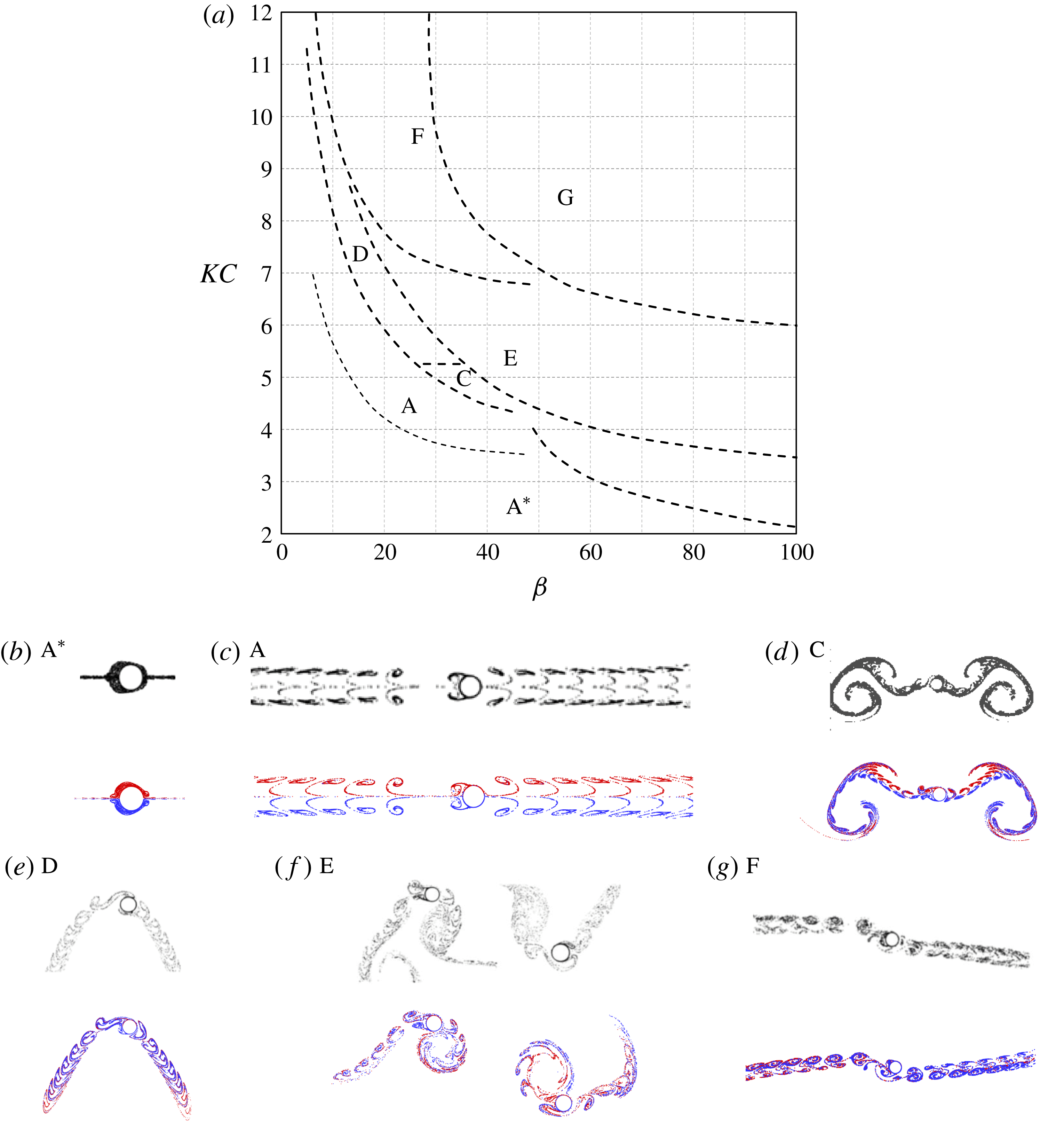
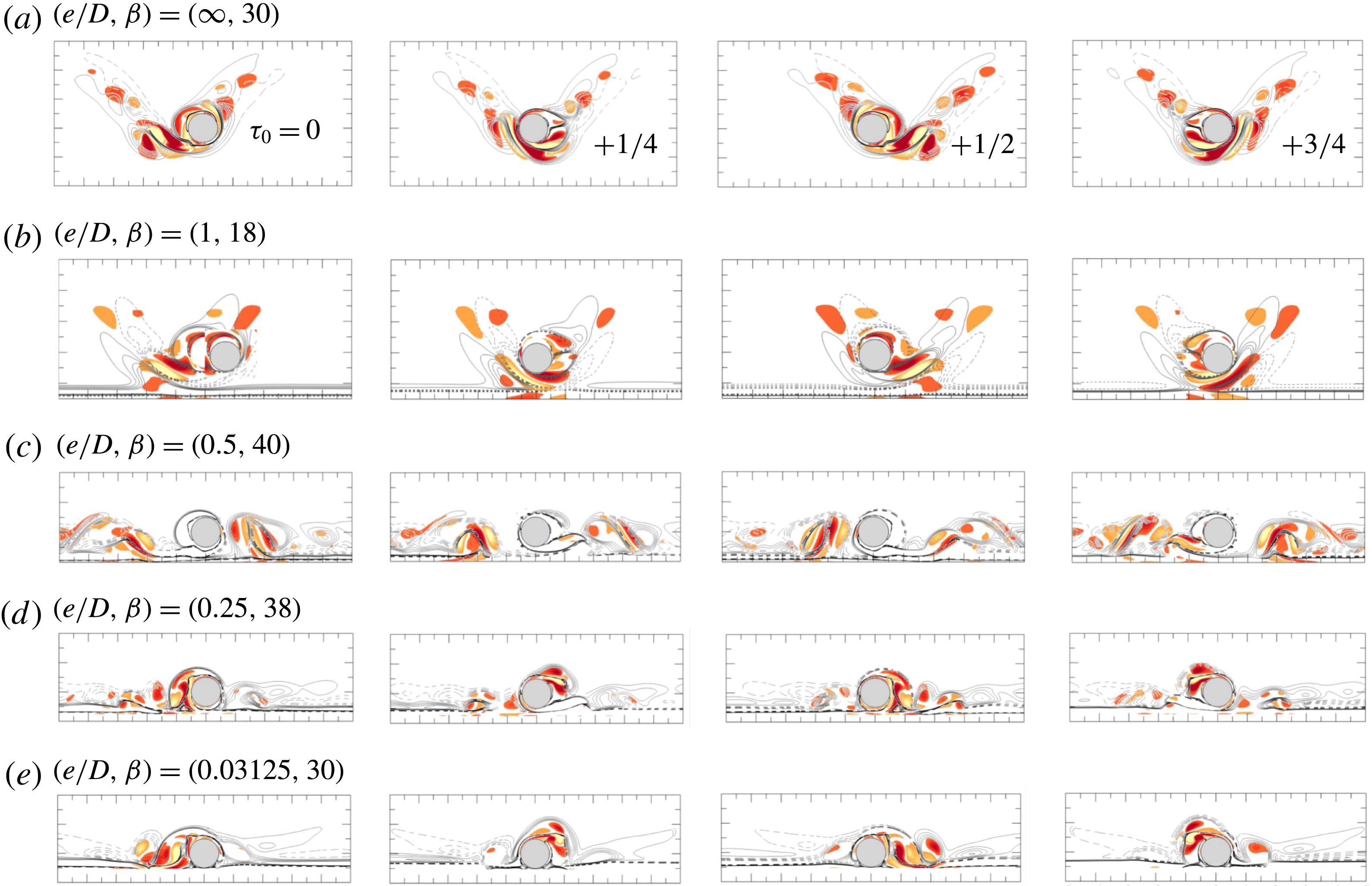
Flow regime map for oscillatory flow past an isolated cylinder reproduced from Tatsuno & Bearman (Reference Tatsuno and Bearman1990) and comparison of streaklines of the present study (red and blue) with those by Zhao & Cheng (Reference Zhao and Cheng2014) and Tong et al. (Reference Tong, Cheng, Zhao and An2015) (grey) at selected parameters. Regime
 $\text{A}^{\ast }$
, symmetric without vortex shedding, streakline at
 $(KC,\unicode[STIX]{x1D6FD})=(3.14,52.8)$
; A, symmetric with vortex shedding, streakline at (11, 7.4); B, longitudinal vortices streaked flow; C, rearrangement of large vortices, streakline at (5, 36); D, transverse street, streakline at (6.28, 22.1); E, transverse street with irregular switching, streakline at (6.28, 25.6) in the 120th (left) and 190th (right) cycle; F, diagonal double pair, streakline at (8.16, 27); and G, circulatory flow streaming that intermittently changes directions. The flows are two-dimensional in regimes A and
 $\text{A}^{\ast }$
, while they are three-dimensional in all other regimes. The streaklines are obtained by constantly releasing massless particles at 120 points around the cylinder surface and integrating their velocity from 32 instantaneous flow fields per period for 8 periods. The particles released from the upper surface of the cylinder are dyed red with the ones from the lower surface dyed blue. It was noted by Tatsuno & Bearman (Reference Tatsuno and Bearman1990) that it is very difficult to determine the onset of vortex shedding, thus the critical curve between regime
 $\text{A}^{\ast }$
and that in regime A is lighter due to the uncertainty.

Oscillatory flow around an isolated circular cylinder has been extensively studied (Bearman et al.
Reference Bearman, Downie, Graham and Obasaju1985; Williamson Reference Williamson1985; Obasaju, Bearman & Graham Reference Obasaju, Bearman and Graham1988; Tatsuno & Bearman Reference Tatsuno and Bearman1990; Justesen Reference Justesen1991; Dütsch et al.
Reference Dütsch, Durst, Becker and Lienhart1998). Tatsuno & Bearman (Reference Tatsuno and Bearman1990) reported a flow regime map comprising of eight flow regimes over
 $KC\leqslant 12$
and
 $\unicode[STIX]{x1D6FD}\leqslant 100$
(reproduced in figure 1). Some typical flow patterns obtained from numerical simulations in the present study are also included for comparison, along with some published numerical results (Zhao & Cheng Reference Zhao and Cheng2014; Tong et al.
Reference Tong, Cheng, Zhao and An2015). A brief description of each of the flow regimes is given in the caption of figure 1 and more details can be found in Tatsuno & Bearman (Reference Tatsuno and Bearman1990). The slight differences between the experimental and numerical results in regime E and regime F (figure 1) are attributed to: (i) regime E flow is aperiodic, implying the streaklines shown at different instants would be different even if the same numerical method and mesh were employed; (ii) the diagonal direction of regime F is arbitrary, which is perhaps affected by bifurcation from the numerical perturbation. Although flows in regimes C, D, E and F are three-dimensional (3-D), two-dimensional (2-D) numerical simulations are still capable of capturing the key characteristics of the flow in the cross-sectional plane (Nehari, Armenio & Ballio Reference Nehari, Armenio and Ballio2004; Elston, Blackburn & Sheridan Reference Elston, Blackburn and Sheridan2006; Tong et al.
Reference Tong, Cheng, Xiong, Draper, An and Lou2017). As summarized by Elston, Sheridan & Blackburn (Reference Elston, Sheridan and Blackburn2004), three symmetry states exist for the flows in the (
 $x,y$
)-plane, which are:
 $$\begin{eqnarray}\displaystyle & \displaystyle K_{x}:\unicode[STIX]{x1D714}_{z}(x,y,t)=-\unicode[STIX]{x1D714}_{z}(x,-y,t), & \displaystyle\end{eqnarray}$$
 $$\begin{eqnarray}\displaystyle & \displaystyle H_{1}:\unicode[STIX]{x1D714}_{z}(x,y,t)=-\unicode[STIX]{x1D714}_{z}(-x,y,t+T/2), & \displaystyle\end{eqnarray}$$
 $$\begin{eqnarray}\displaystyle & \displaystyle H_{2}:\unicode[STIX]{x1D714}_{z}(x,y,t)=\unicode[STIX]{x1D714}_{z}(-x,-y,t+T/2). & \displaystyle\end{eqnarray}$$
Here
 $\unicode[STIX]{x1D714}_{z}$
is the spanwise vorticity. Figure 1 shows that the cross-sectional flows hold the
 $K_{x}$
symmetry (or the reflection symmetry) in regimes A and
 $\text{A}^{\ast }$
, the
 $H_{1}$
spatio-temporal symmetry in regimes B and D and the
 $H_{2}$
spatio-temporal symmetry in regime F. Irregular transverse vortex shedding and turbulent motions are observed in regime G without any trace of the above-defined symmetry states.
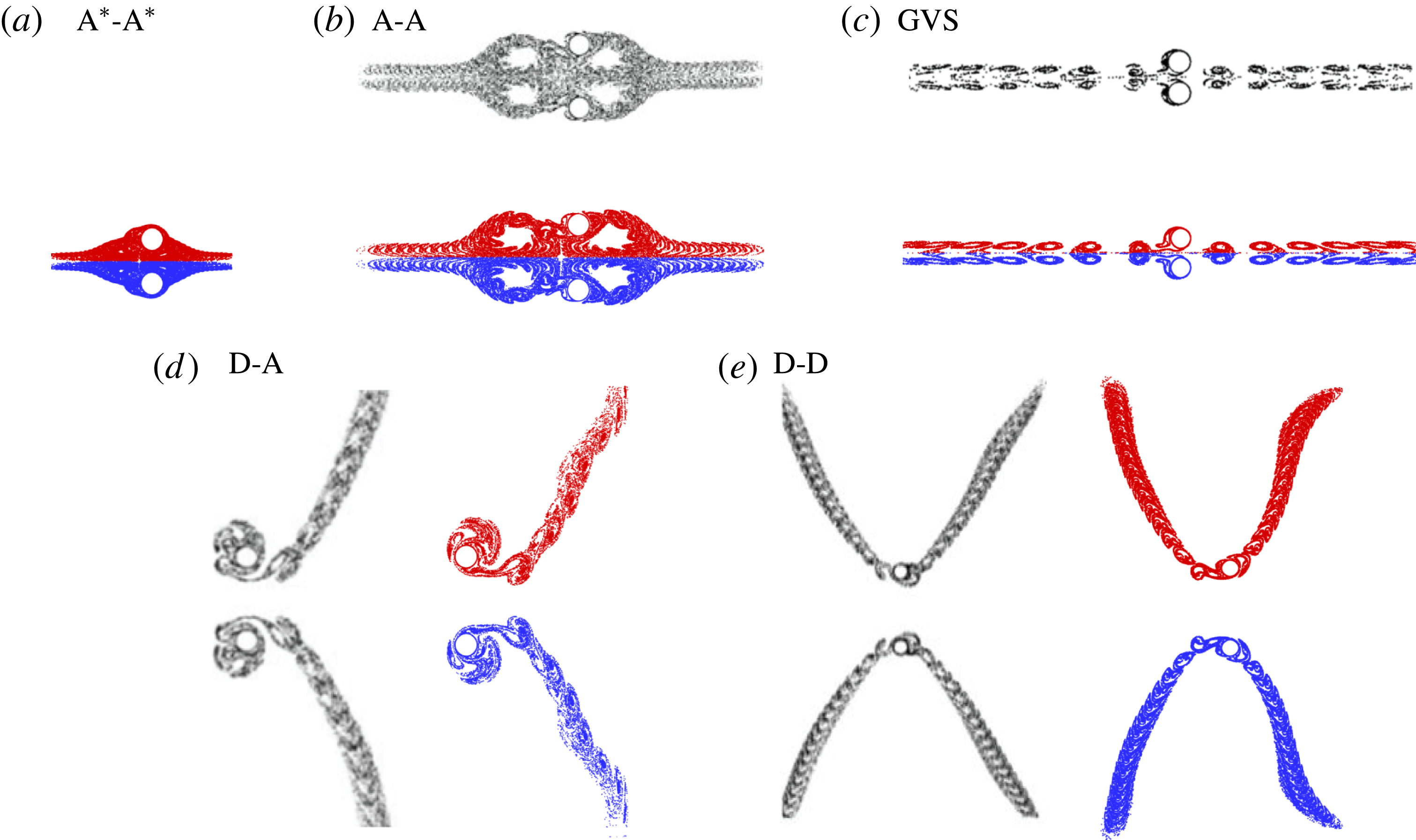
Flow regimes illustrated by streaklines for oscillatory flow past two side-by-side cylinders. The ones with red and blue colours are based on the present simulations, and those with grey are from Zhao & Cheng (Reference Zhao and Cheng2014) at the same control parameters. (a) Regime
 $\text{A}^{\ast }-\text{A}^{\ast }$
at
 $(G/D,KC,\unicode[STIX]{x1D6FD})=(1,3,50)$
; (b) regime A-A at (2, 5, 30); (c) regime GVS at (0.5, 5, 30); (d) regime D-A at (3, 7, 21.4); (e) regime D-D at (4, 6, 25).

Elston et al. (Reference Elston, Sheridan and Blackburn2004) carried out a Floquet stability analysis and direct numerical simulation (DNS) to investigate the
 $K_{x}$
symmetry breaking within the range of
 $KC\leqslant 10$
and
 $\unicode[STIX]{x1D6FD}\leqslant 100$
. The predicted marginal curve from the 2-D analysis agrees very well with the regime boundary reported by Tatsuno & Bearman (Reference Tatsuno and Bearman1990) for flow transitions from regime A to D, A to C and B to E. Elston et al. (Reference Elston, Blackburn and Sheridan2006) further detected a ‘freezing point’ along the marginal curve, where the critical complex-conjugate pair of Floquet multipliers coalesce at a single real value and the instability mode becomes synchronous with the base flow. At low
 $\unicode[STIX]{x1D6FD}$
below the freezing point, the flow instability is synchronous with the base flow, while at high
 $\unicode[STIX]{x1D6FD}$
above the point the instability is quasi-periodic with a secondary period that is larger than the period of flow oscillations (Elston et al.
Reference Elston, Blackburn and Sheridan2006).
Zhao & Cheng (Reference Zhao and Cheng2014) investigated the oscillatory flow regimes around two side-by-side cylinders, which is somewhat relevant to the present study in topology. The streaklines of some selected flow regimes are reproduced in figure 2 to facilitate the following discussion. Specifically, the flow regimes that have been identified for a single cylinder were also observed in the two-cylinder system. More interestingly, the flow may show features of a combination of two different regimes, as in regime D-A (figure 2 d), which is a spatial combination of regime A at one side of the cylinder bundle, but regime D at the other side. In addition, vortex shedding from the gap between the two cylinders dominates when the gap distance is relatively small, resulting in the gap vortex shedding (GVS) regime (figure 2 c).
To investigate the effect of wall proximity, Rao et al. (Reference Rao, Thompson, Leweke and Hourigan2013) studied the onset of 2-D instability and transition to three dimensions of the steady incoming flow past a circular cylinder translating parallel to a no-slip wall at different gap heights by DNS and Floquet analysis. In addition, the effect of cylinder rotations was considered by Rao et al. (Reference Rao, Stewart, Thompson, Leweke and Hourigan2011) and Rao et al. (Reference Rao, Thompson, Leweke and Hourigan2015). For oscillatory flow, Sarpkaya (Reference Sarpkaya1976) measured the drag, inertia and lift coefficients acting on a circular cylinder placed at various gap ratios for
 $2\leqslant KC\leqslant 40$
and
 $4000\leqslant Re\leqslant 25\,000$
. The drag and inertia coefficients and the oscillation magnitude of lift forces were found to increase as
 $e/D$
was reduced. For a wall-mounted circular cylinder (i.e.
 $e/D=0$
), the direction of the lift force was found to be always away from the wall. In contrast, a large lift force towards the wall was observed at small
 $e/D$
. Sumer & Fredsøe (Reference Sumer and Fredsøe1997) studied the correlation between temporal variations of force coefficients and vortex motions within
 $0<e/D<25$
. Scandura, Armenio & Foti (Reference Scandura, Armenio and Foti2009) performed a 3-D DNS for
 $0.25\leqslant e/D\leqslant 1.5$
at
 $KC=10$
,
 $\unicode[STIX]{x1D6FD}=20$
and 50. It was found that a reduction of
 $e/D$
leads to a transition from an aperiodic to a cycle-to-cycle periodic vortex motion. The comparison between the 2-D and 3-D results supports the use of the 2-D model for the study of oscillatory flow around cylinders placed close to a plane wall, even at
 $Re=500$
.
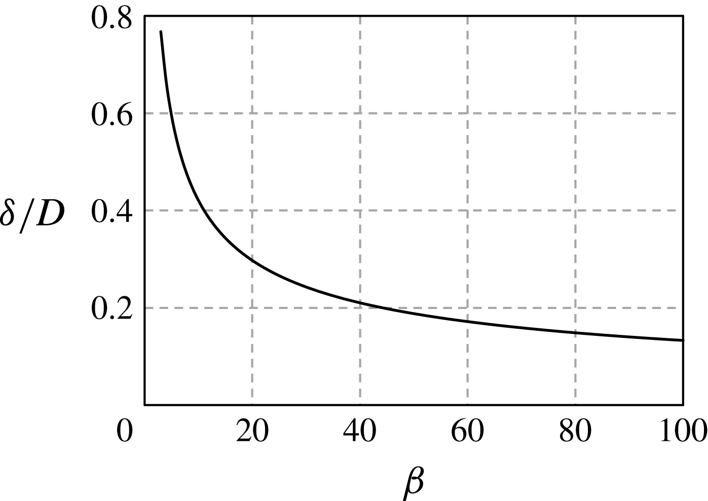
The variation of normalized thickness of the Stokes layer (
 $\unicode[STIX]{x1D6FF}/D$
) with the Stokes number,
 $\unicode[STIX]{x1D6FD}$
, covered in this study.

The thickness of the wall boundary layer has been long believed to be significant for steady flow (Zdravkovich Reference Zdravkovich1985). However, to date, little attention has been paid to the influence of the thickness of the Stokes boundary layer
 $\unicode[STIX]{x1D6FF}$
on oscillatory flows around a cylinder near a plane boundary, possibly because
 $\unicode[STIX]{x1D6FF}$
is relatively small at high
 $\unicode[STIX]{x1D6FD}$
(or
 $Re$
) values. However, this may not be the case for the flow with relatively low
 $\unicode[STIX]{x1D6FD}$
(or
 $Re$
) values where the influence of
 $e/\unicode[STIX]{x1D6FF}$
on the flow may become important. This somewhat motivates the present study, where the flow is investigated over the parameter ranges
 $3\leqslant KC\leqslant 12$
,
 $Re\leqslant 300$
and
 $0.03125\leqslant e/D\leqslant 2.0$
. The variation of the normalized thickness of the Stokes boundary layer,
 $\unicode[STIX]{x1D6FF}/D$
, with
 $\unicode[STIX]{x1D6FD}$
is shown in figure 3, where
 $$\begin{eqnarray}\frac{\unicode[STIX]{x1D6FF}}{D}=\frac{3\unicode[STIX]{x03C0}}{4}\left(\frac{1}{\unicode[STIX]{x03C0}\unicode[STIX]{x1D6FD}}\right)^{1/2}.\end{eqnarray}$$
This is adapted and modified from (11) of Carstensen, Sumer & Fredsøe (Reference Carstensen, Sumer and Fredsøe2010). It should be noted that (1.5) is only valid for an undisturbed plane oscillatory boundary layer flow. The thickness of the plane boundary layer beneath the cylinder would inevitably change with the approach of the cylinder.
The remainder of the paper is organized in the following manner. In § 2, the mathematical models are introduced. In § 3, the regime maps are given, followed by discussions on the vortex motions and hydrodynamic forces for each of the regimes. The hysteresis phenomenon is investigated in § 4, and the 3-D effects are briefly shown in § 5. Finally, the concluding remarks are given in § 6. Detailed validations of numerical methods are presented in the appendix.
2 Computational methods
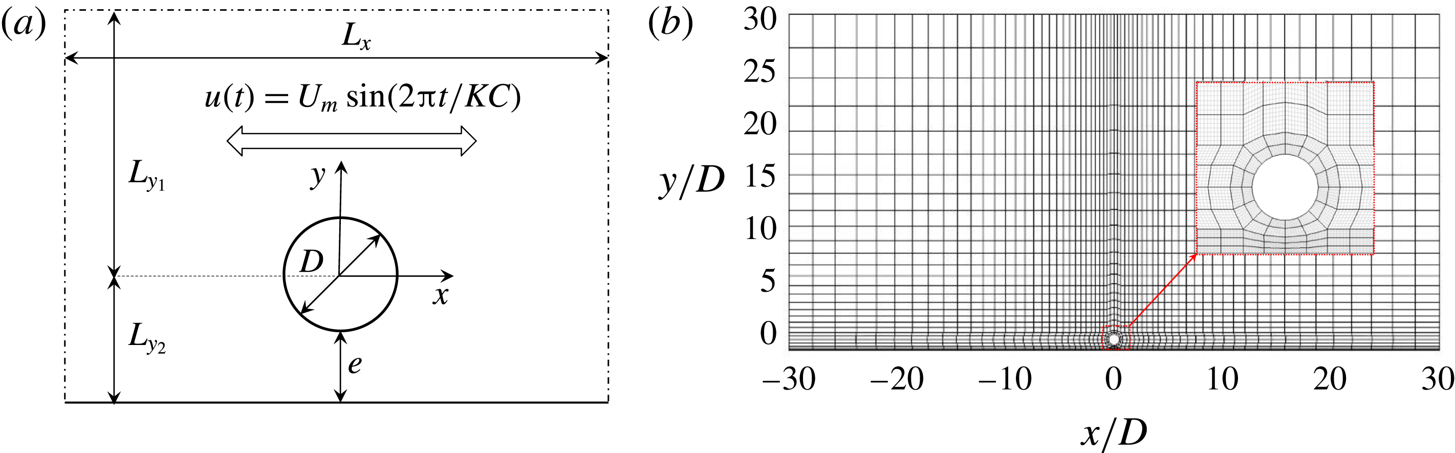
The problem investigated in this study is illustrated in figure 4. A frame of reference is defined with its origin at the centre of the cylinder and its axes are referred to as (
 $x,y$
). The size of computation domain is represented by
 $L_{x}\times (L_{y1}+L_{y2})$
, where
 $L_{x}$
is the distance between streamwise boundaries, and
 $L_{y1}$
and
 $L_{y2}$
are respectively the lengths from the upper and lower boundaries to the
 $x$
-axis (i.e.
 $y=0$
). The fluid motion is governed by the incompressible Navier–Stokes (N–S) equations, expressed in dimensionless form as,
 $$\begin{eqnarray}\displaystyle & \displaystyle \frac{\unicode[STIX]{x2202}\boldsymbol{u}}{\unicode[STIX]{x2202}t}=-(\boldsymbol{u}\boldsymbol{\cdot }\unicode[STIX]{x1D735})\boldsymbol{u}-\unicode[STIX]{x1D6FB}p+Re^{-1}\unicode[STIX]{x1D6FB}^{2}\boldsymbol{u}, & \displaystyle\end{eqnarray}$$
 $$\begin{eqnarray}\displaystyle & \displaystyle \unicode[STIX]{x1D6FB}\boldsymbol{\cdot }\boldsymbol{u}=0, & \displaystyle\end{eqnarray}$$
where
 $\boldsymbol{u}=(u,v)$
is the velocity field and
 $p(x,y,t)$
is the pressure field. The velocity components,
 $u(x,y,t)$
and
 $v(x,y,t)$
, are in the
 $x$
- and
 $y$
-directions, respectively. The velocity components have been normalized by maximum free-stream velocity
 $U_{m}$
and the axes are normalized by cylinder diameter
 $D$
.
(a) Schematic illustration of the geometry settings; and (b) a typical mesh configuration along with a close-up view at
 $e/D=0.5$
with
 $N_{p}=7$
. The
 $h$
-type elements are given in black and
 $p$
-type elements are shown in grey.

The above N–S equations are solved using a spectral/
 $hp$
element method embedded in an open source code, Nektar++ (Cantwell et al.
Reference Cantwell, Moxey, Comerford, Bolis, Rocco, Mengaldo, De Grazia, Yakovlev, Lombard and Ekelschot2015). For a 2-D mesh, the total resolution is determined by the distribution of
 $h$
-type elements and interpolant order
 $N_{p}$
for the
 $p$
-type refinement. The Fourier-spectral/
 $hp$
method is adopted to solve the three-dimensional N–S equations, although only a few 3-D cases are conducted and reported in § 5. The 3-D simulations consist of using a spectral/
 $hp$
element method to spatially discretize the N–S equations in the (
 $x,y$
)-plane and a Fourier expansion in the
 $z$
-direction to reveal 3-D features of the flow. Therefore, the velocity vector is written in the form of the Fourier expansion with a total node number of
 $2N$
in the spanwise direction, where each Fourier component
 $\hat{\boldsymbol{u}}_{m}$
is a complex mode at the discrete wavenumber
 $k=2\unicode[STIX]{x03C0}mD/L_{z}$
, where
 $m(=0,1,\ldots ,N-1)$
is the Fourier mode index. Hence only a 2-D mesh is required for the Fourier-spectral/
 $hp$
approach. A more elaborate introduction to this numerical method can be found in Bolis (Reference Bolis2013).
The boundary conditions employed in the simulation are described briefly. The free-stream velocity is specified as
 $u_{\infty }(t)=U_{m}\text{sin}(2\unicode[STIX]{x03C0}t/KC)$
and
 $v_{\infty }=0$
at the streamwise boundaries (inlet and outlet) and the upper open boundaries. Zero Dirichlet velocity boundary conditions are applied on the cylinder surface and the plane boundary. A high-order Neumann pressure boundary condition is imposed for all domain boundaries, as described by Blackburn & Henderson (Reference Blackburn and Henderson1999). Initial conditions of zero flow velocity and pressure are employed in the simulations unless otherwise specified. Attentions have been paid to the choice of the inlet and outlet boundary conditions because of the different choices reported in the literature. For examples, Shen & Chan (Reference Shen and Chan2013) adopted the Dirichlet velocity boundary condition at the inlet and Neumann velocity boundary condition at the outlet. Scandura et al. (Reference Scandura, Armenio and Foti2009) employed a periodic boundary condition in the streamwise direction. An, Cheng & Zhao (Reference An, Cheng and Zhao2010) adopted the Dirichlet velocity boundary condition on both inlet and outlet boundaries. To examine these three choices, a validation test is carried out. It is found that the numerical results are independent of the choice of inlet/outlet boundary conditions, as long as the boundaries are set sufficiently far away from the cylinder to allow a fully developed oscillatory boundary layer flow in the neighbourhood of the cylinder. It is also found that the Stokes boundary layer is normally fully developed within a distance of approximately
 $10\unicode[STIX]{x1D6FF}({\sim}2D)$
from the inlet/outlet boundaries. A relatively long streamwise domain length (
 ${>}40D$
) is adopted to avoid potential influence from the inlet/outlet boundary conditions.
Temporal Floquet analysis is carried out to examine the growth rate of velocity and pressure perturbations (
 $\boldsymbol{u}^{\prime },p^{\prime }$
) for a
 $T$
-periodic base flow
 $\boldsymbol{U}$
. The linearized Navier–Stokes and continuity equations of velocity and pressure perturbations read:
 $$\begin{eqnarray}\displaystyle & \displaystyle \frac{\unicode[STIX]{x2202}\boldsymbol{u}^{\prime }}{\unicode[STIX]{x2202}t}=-\boldsymbol{U}\boldsymbol{\cdot }\unicode[STIX]{x1D6FB}\boldsymbol{u}^{\prime }-\boldsymbol{u}^{\prime }\boldsymbol{\cdot }\unicode[STIX]{x1D6FB}\boldsymbol{U}-\unicode[STIX]{x1D6FB}p^{\prime }+Re^{-1}\unicode[STIX]{x1D6FB}^{2}\boldsymbol{u}^{\prime }, & \displaystyle\end{eqnarray}$$
 $$\begin{eqnarray}\displaystyle & \displaystyle \unicode[STIX]{x1D6FB}\boldsymbol{\cdot }\boldsymbol{u}^{\prime }=0, & \displaystyle\end{eqnarray}$$
where the perturbations are numerically determined with respect to the base flow through an iterative approach (Henderson & Barkley Reference Henderson and Barkley1996; Elston et al.
Reference Elston, Sheridan and Blackburn2004, Reference Elston, Blackburn and Sheridan2006). Perturbation solutions can be written as a sum of components
 $\tilde{\boldsymbol{u}}(t_{0})\text{exp}\unicode[STIX]{x1D70E}(t-t_{0})$
, where
 $\tilde{\boldsymbol{u}}(t_{0})$
is a
 $T$
-periodic Floquet eigenfunction evaluated at an arbitrary phase
 $t_{0}$
, and
 $\unicode[STIX]{x1D70E}$
is a Floquet exponent. The Floquet multiplier
 $\unicode[STIX]{x1D707}\equiv \text{exp}(\unicode[STIX]{x1D70E}T)$
can be either real or a complex-conjugate pair. Instability occurs when the Floquet multiplier
 $|\unicode[STIX]{x1D707}|>1$
.
The global stability analysis method employed in this study is generally the same as the method reported by Barkley & Henderson (Reference Barkley and Henderson1996) and Elston et al. (Reference Elston, Blackburn and Sheridan2006), except for the method of enforcing the symmetry in the base flow. In Elston et al. (Reference Elston, Sheridan and Blackburn2004), reflection symmetry was imposed on the base flow to investigate
 $K_{x}$
symmetry breaking. Since
 $H_{1}$
symmetry breaking is the focus of this study, the method of enforcing symmetry in the base flow reported by Elston et al. (Reference Elston, Sheridan and Blackburn2004) is not applicable in this study. For this reason, a new stabilization technique is proposed to enforce
 $H_{1}$
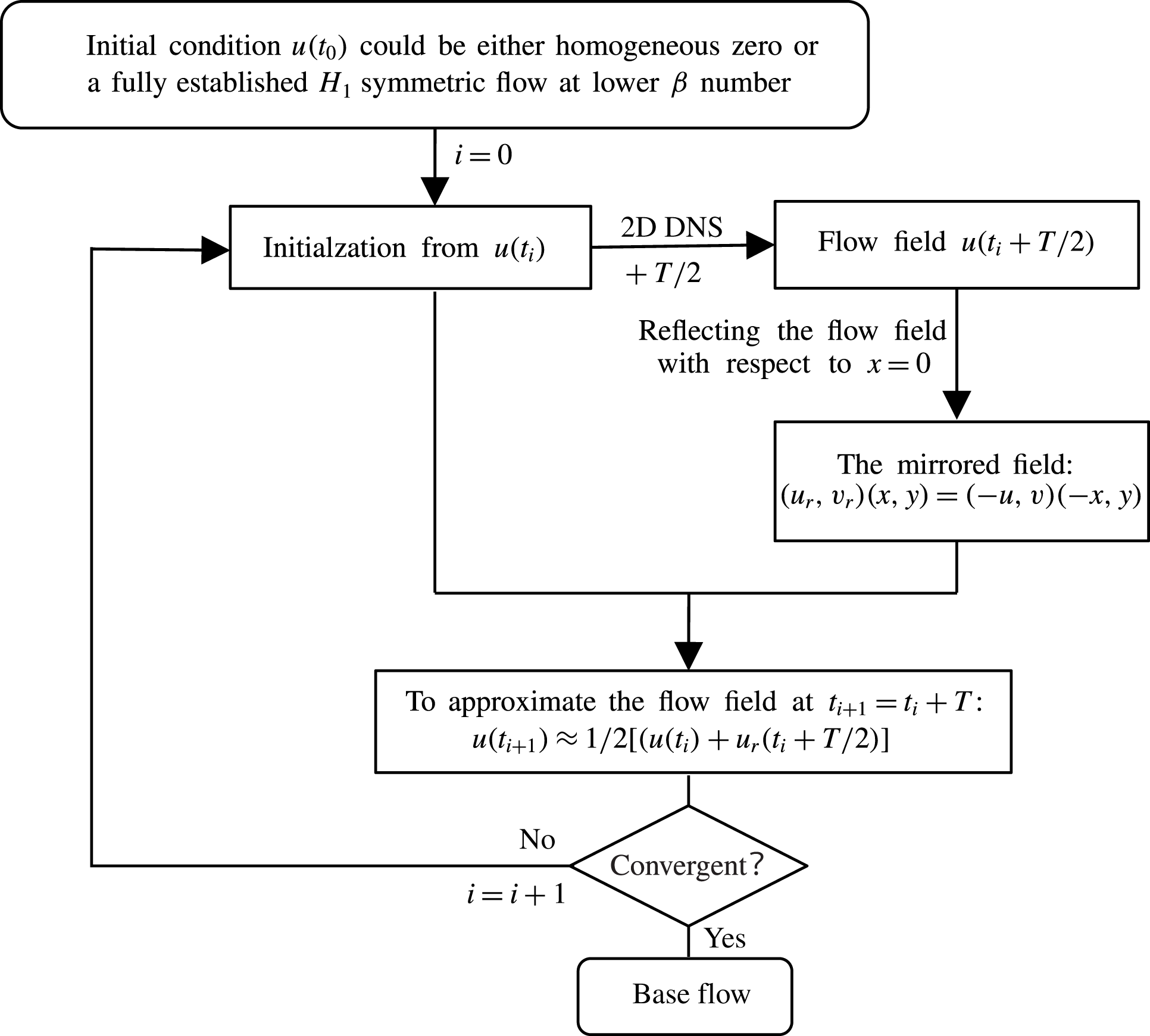
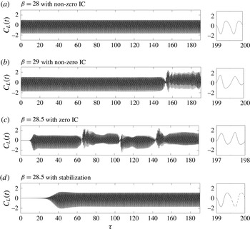
symmetry of the base flow, which is introduced in figure 32 in the appendix.
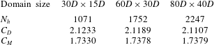
A careful mesh sensitivity study was carried out to determine the size of the computational domain and the order of interpolant (
 $N_{p}$
) used, which is also detailed in the appendix. The chosen values of
 $L_{x}\times L_{y1}=60D\times 30D$
and
 $N_{p}=7$
are comparable with those employed in previous relevant studies (Elston et al.
Reference Elston, Blackburn and Sheridan2006; Scandura et al.
Reference Scandura, Armenio and Foti2009; An et al.
Reference An, Cheng and Zhao2010). The Floquet analysis model is also validated against that used in Elston et al. (Reference Elston, Blackburn and Sheridan2006) with satisfactory agreement.
3 Classification of flow regimes
3.1 Flow regimes
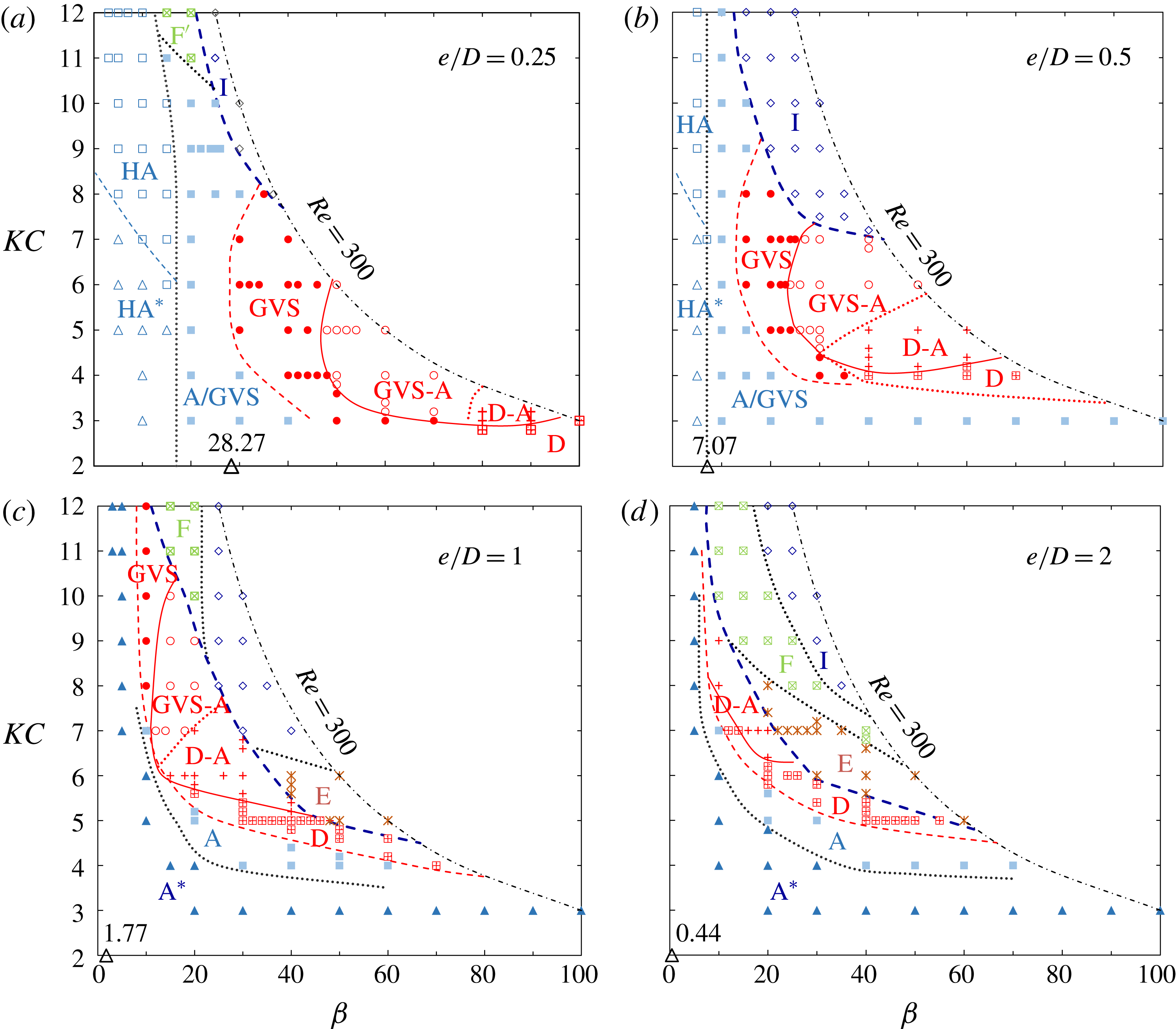
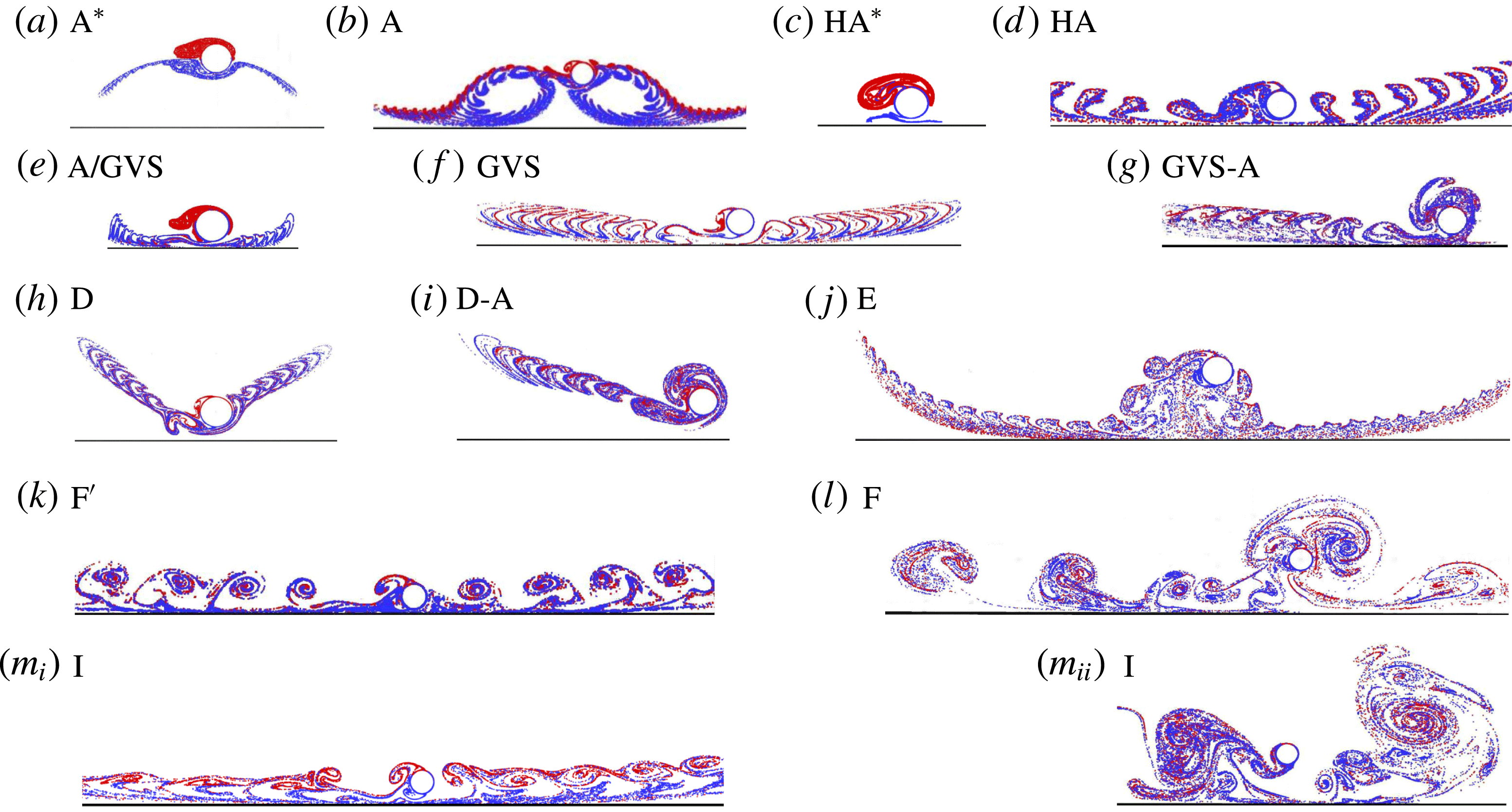
The flow regimes are mapped out in figure 5 at
 $e/D=0.25$
, 0.5, 1 and 2 in
 $(KC,\unicode[STIX]{x1D6FD})$
-space for
 $3\leqslant KC\leqslant 12$
and
 $\unicode[STIX]{x1D6FD}\leqslant 300/KC$
, while a representative flow pattern for each identified regime is given in figure 6. The
 $KC$
and
 $\unicode[STIX]{x1D6FD}$
resolutions used to generate figure 5 range from 0.1 to 1 and from 1 to 10 respectively. Fine resolution is employed to identify the regime boundaries.
Classifications of oscillatory flow regimes around a circular cylinder above a plane boundary at different gap ratios based on 2-D DNS results. The boundary lines are obtained based on the flow identification at discrete data points, which are marked with different symbols and colours along with regime names. The synchronous and asynchronous regimes with regard to the oscillatory flow are distinguished by the bold dashed line (– – – blue). Only the red solid lines (—— red) represent an abrupt change between regimes, while all others represent a gradual transition between adjacent regimes. The upper limit of
 $Re=300$
for the current research is represented by dot-dashed lines (– ⋅ – ⋅ –). The open triangle marker (▵) on the horizontal axis indicates the corresponding Stokes number where the thickness of undisturbed Stokes boundary layer calculated by (1.5) is identical to the gap size,
 $e$
.

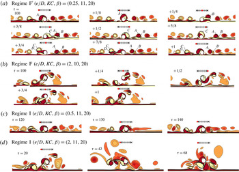
Flow patterns represented by streaklines in different flow regimes for oscillatory flow around a circular cylinder above a no-slip plane boundary: (a) regime
 $\text{A}^{\ast }$
at
 $(e/D,KC,\unicode[STIX]{x1D6FD})=(2,4,20)$
; (b) A at (2, 5, 30); (c)
 $\text{HA}^{\ast }$
at (0.25, 4, 10); (d) HA at (0.25, 10, 10) (see movie 1 available at https://doi.org/10.1017/jfm.2018.164); (e) transitional regime A/GVS at (0.5, 4, 20); (f) GVS at (0.5, 6, 20) (see movie 2); (g) GVS-A at (0.5, 6, 30) (see movie 3); (h) D at (0.5, 4, 50); (i) D-A at (1, 6, 25); (j) E at (2, 6, 30) (see movie 4); (k)
 $\text{F}^{\prime }$
at (0.25, 11, 20) (see movie 5); (l) F at (2, 10, 20) (see movie 6); (
 $m_{i}$
) I at (0.5, 11, 20) and (
 $m_{ii}$
) I at (2, 11, 20).

A number of distinctive flow regimes are observed, as shown in figures 5 and 6. The naming of flow regimes follows the conventions previously reported in the literature as much as possible. Among these, regimes
 $\text{A}^{\ast }$
, A, D, E, F are similar to those found in oscillatory flow around an isolated circular cylinder (Tatsuno & Bearman Reference Tatsuno and Bearman1990), and regimes GVS and D-A are similar to those identified for two side-by-side cylinders (Zhao & Cheng Reference Zhao and Cheng2014). Although these flows are not strictly identical to those found previously, the naming convention is retained to avoid creating too many new regime names. The regimes
 $H\text{A}^{\ast }$
, HA, GVS-A and I are unique for oscillatory flow around a circular cylinder near a plane boundary. Here the prefix ‘H’ stands for ‘half’ because of its spatial similarity to a half of regime
 $\text{A}^{\ast }$
or A structure for an isolated cylinder. The superscript ‘
 $^{\ast }$
’ indicates no vortex shedding, which is inherited from the definition of regime
 $\text{A}^{\ast }$
in previous studies and ‘I’ represents ‘irregularity’, where no clear cycle-to-cycle periodicity is observed. A transitional region between regimes
 $\text{HA}^{\ast }/\text{HA}$
and GVS is marked with A/GVS in the regime map at
 $e/D=0.25$
and 0.5, because the flow possesses the features of both regimes. In general, an abrupt change is only observed along boundary lines between regime GVS to GVS-A and D to D-A (or E) within the parameter space.
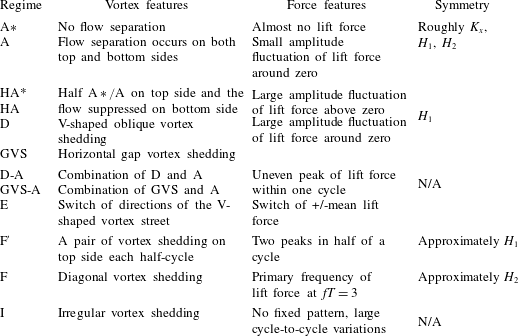
The classification of flow regimes is primarily based on visual observations of instantaneous vorticity contours and the streaklines of the 2-D DNS results, with the aid of information derived from hydrodynamic forces. Each of the flow regimes is characterized by unique vortex shedding features, force characteristics, synchronization and symmetry states. The main criteria used for the classification are summarized in table 1.
The features and the criteria of identification for each flow regime.

A prominent feature is that the flow regimes are highly dependent on
 $e/D$
. The flow regime map for
 $e/D=2$
tends to resemble the map of an isolated cylinder shown in figure 1, suggesting the weak influence of the plane boundary at
 $e/D>2$
. As
 $e/D$
is reduced, the regime maps change significantly, especially at the lower end of the
 $\unicode[STIX]{x1D6FD}$
range. The newly identified flow regimes (
 $\text{HA}^{\ast }$
, HA, GVS-A and I) are either associated with small
 $e/D$
or/and low
 $\unicode[STIX]{x1D6FD}$
values. The typical flow features in each regime will be explained below based on vorticity contours and hydrodynamic forces. In the present study, the inline force coefficient
 $C_{x}$
and lift coefficient
 $C_{L}$
are used to plot Lissajous phase diagrams. The force coefficients are defined as
 $C_{x}=F_{x}/(0.5\unicode[STIX]{x1D70C}DU_{m}^{2})$
and
 $C_{L}=F_{y}/(0.5\unicode[STIX]{x1D70C}DU_{m}^{2})$
, where
 $\unicode[STIX]{x1D70C}$
is the fluid density.
 $F_{x}$
and
 $F_{y}$
are the inline and transverse forces respectively and are obtained by integrating pressure and viscous forces over the surface of the cylinder. The flow states of symmetry can be identified based on Lissajous phase diagram of
 $C_{x}-C_{L}$
: (i) a closed loop suggests cycle-to-cycle periodicity; (ii) a horizontal line implies
 $K_{x}$
symmetry; (iii) a symmetric Lissajous phase diagram about
 $C_{x}=0$
means
 $H_{1}$
symmetry; and (iv) a symmetric Lissajous phase diagram about (
 $0,0$
) indicates
 $H_{2}$
symmetry.
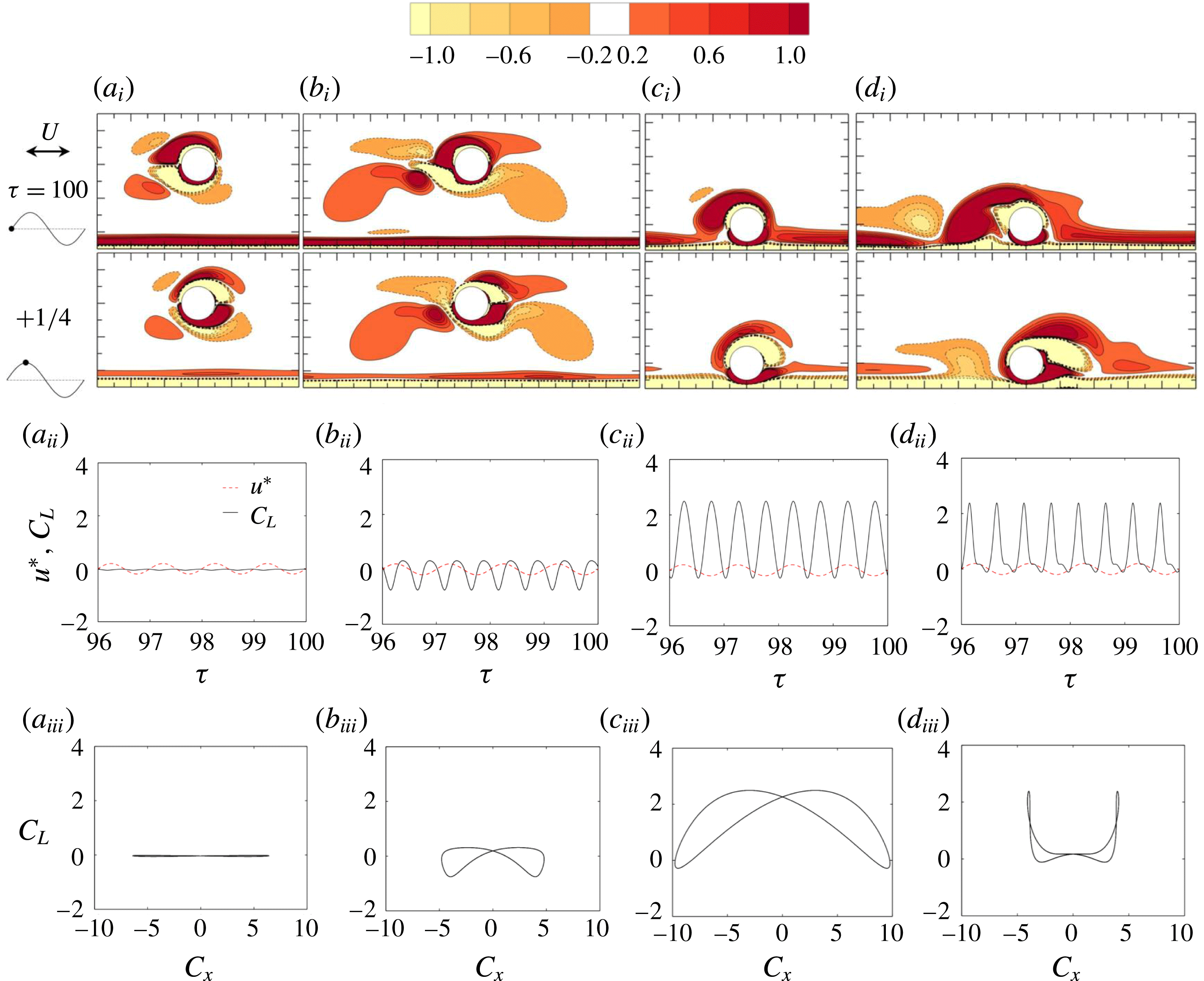
From top to bottom are (
 $i$
) the instantaneous contours of
 $\unicode[STIX]{x1D714}_{z}$
between
 $\unicode[STIX]{x1D714}_{z}=1$
(light colours) and
 $+1$
(dark ones) with cutoff level
 $\pm 0.2$
(this applies to other vorticity contours unless otherwise specified), and the phase
 $\unicode[STIX]{x1D70F}_{0}$
of sampling is indicated by
 $\bullet$
in the sinusoidal velocity signal; (
 $ii$
) the transient trace of
 $C_{L}$
(solid black lines) along with scaled free-stream velocity
 $u^{\ast }=u_{\infty }/5$
(dashed red lines); and (
 $iii$
) Lissajous phase diagram of
 $C_{x}{-}C_{L}$
. From left to right are (a) regime
 $\text{A}^{\ast }$
at
 $(e/D,KC,\unicode[STIX]{x1D6FD})=(2,4,20)$
; (b) regime A at (2, 5, 30); (c) regime H
 $\text{A}^{\ast }$
at (0.25, 4, 10); and (d) regime HA at (0.25, 10, 10). Due to the strict
 $H_{1}$
symmetry, only two snapshots at
 $\unicode[STIX]{x1D70F}_{0}=0$
and 1/4 are shown in (
 $i$
) and those at
 $\unicode[STIX]{x1D70F}_{0}=1/2$
and 3/4 can be obtained by (1.3).

3.1.1 Regimes
 $A^{\ast }$
, A,
$HA^{\ast }$
and HA


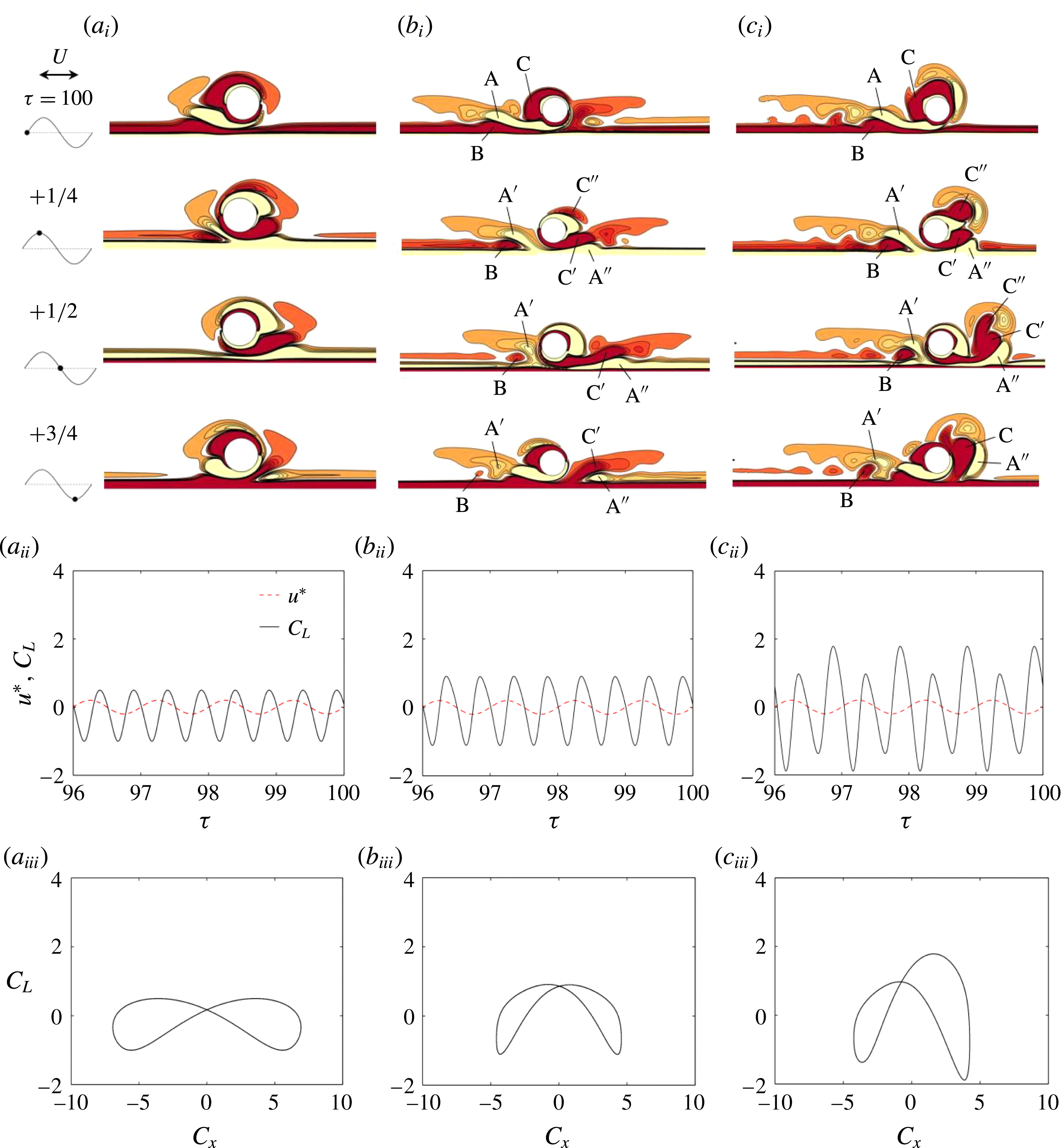
As shown in figure 7(a,b), the flows in regime
 $\text{A}^{\ast }$
/A resemble their counterparts around an isolated cylinder (figure 1). Due to the proximity of the plane boundary, there is a slight asymmetry in the flow about the oscillating axis, which gives rise to a non-zero lift in regime A.
The newly reported regimes
 $\text{HA}^{\ast }$
/HA (figure 7
c,d) only exist for
 $\unicode[STIX]{x1D6FF}/e>1$
and are similar to the flow observed by Sumer et al. (Reference Sumer, Jensen and Fredsøe1991) at
 $e/D=0$
and
 $KC=4$
. Regime
 $\text{HA}^{\ast }$
is characterized by vortices attached to the upper half of the cylinder surface, without discernible vortex shedding. The streaklines (figure 6
c) from the upper surface are convected in a similar way to the upper half of regime
 $\text{A}^{\ast }$
(figure 6
a), but the streaklines on the bottom half of the cylinder surface are quite different and form a narrow horizontal strip moving along with the Stokes boundary layer. The particles released from the upper and lower cylinder surfaces do not mix, suggesting a rather weak interaction between the shear layers formed on the cylinder surface. Figure 7(c) for regime
 $\text{HA}^{\ast }$
flow illustrates a regular and smooth temporal variation of the lift with a positive non-zero mean. The amplitude of
 $C_{x}$
is larger than its counterpart in regime A/
 $\text{A}^{\ast }$
.
Same as figure 7 but (a) transitional regime A/GVS at
 $(e/D,KC,\unicode[STIX]{x1D6FD})=(0.5,4,20)$
; (b) regime GVS at (0.5, 6, 20); and (c) regime GVS-A at (0.5, 6, 30).

The flow features observed in regime HA (figure 7
d) are characterized by the shedding of one vortex from the top side in each half of an oscillation period, while the formation of the vortex on the gap side is suppressed due to the Stokes boundary layer. The streaklines (figure 6
d) show that fluid particles are transported nearly horizontally but with an upwards inclination. The variation of
 $C_{L}$
(figure 7
d) is strong and the value is almost always positive.
3.1.2 Regimes GVS, GVS-A, D and D-A
Regimes GVS and GVS-A only emerge at
 $e/D\leqslant 1$
, where the plane boundary has a significant influence on the flow around the cylinder. These flow patterns, along with the transitional regime A/GVS, are illustrated in figure 8. By comparing figure 8(a, b), it is obvious that the gap vortex shedding strengthens with increasing
 $KC$
. The streakline patterns, shown in figure 6(e,f), also show that the particles are convected horizontally with a slight upwards inclination due to the gap flow.
Regimes GVS and A may coexist due to the influence of wall proximity, forming a combined regime GVS-A. The flow is in regime GVS at the left-hand side in figure 8(c), but remains in regime A at the other side. The flow structure is asymmetric about
 $x=0$
, which was also observed by Sumer et al. (Reference Sumer, Jensen and Fredsøe1991) and An et al. (Reference An, Cheng and Zhao2010) for
 $4<KC<7$
and
 $e/D<1$
.
Figure 8(b,c) compares the shedding and movement of a pair of vortices, A and B (shed from the gap in the previous half-cycle) and a vortex C (attached to the upper cylinder surface) for GVS and GVS-A in a typical oscillation period. After the flow reversal, vortex A is split into two vortices
 $\text{A}^{\prime }$
and
 $\text{A}^{\prime \prime }$
. The vortex C is also split into two parts during the acceleration phase with the major part
 $\text{C}^{\prime }$
flowing through the gap and the minor part
 $\text{C}^{\prime \prime }$
washing over the upper surface. The major difference between GVS and GVS-A at
 $\unicode[STIX]{x1D70F}=t/T=100.25$
is that
 $\text{C}^{\prime }$
is stronger than
 $\text{C}^{\prime \prime }$
in GVS, opposite to GVS-A. The vortices
 $\text{A}^{\prime }$
and B remain at the left-hand side while the vortices
 $\text{A}^{\prime \prime }$
and
 $\text{C}^{\prime }$
are convected to the right-hand side. For GVS flow, vortices
 $\text{C}^{\prime }$
and
 $\text{A}^{\prime \prime }$
in the second half of the cycle are spatio-temporal mirror images of the vortices A and B in the previous half-cycle. Successive vortex pairs are convected away from the gap, resulting in a vortex street at either side of the cylinder, as shown in figure 6(f). On the other hand, the vortices
 $\text{C}^{\prime }$
and
 $\text{A}^{\prime \prime }$
roll up at
 $\unicode[STIX]{x1D70F}=100.5$
for GVS-A, merging with vortex
 $\text{C}^{\prime \prime }$
, and are washed back towards the cylinder during the flow reversal. The flow in regime GVS-A is still strictly cycle-to-cycle periodic, as can be seen from the closed loop Lissajous phase diagram shown in figure 8(c), but breaks
 $H_{1}$
symmetry. Two cycles of lift fluctuation are observed in each flow period with two peaks of different magnitudes.
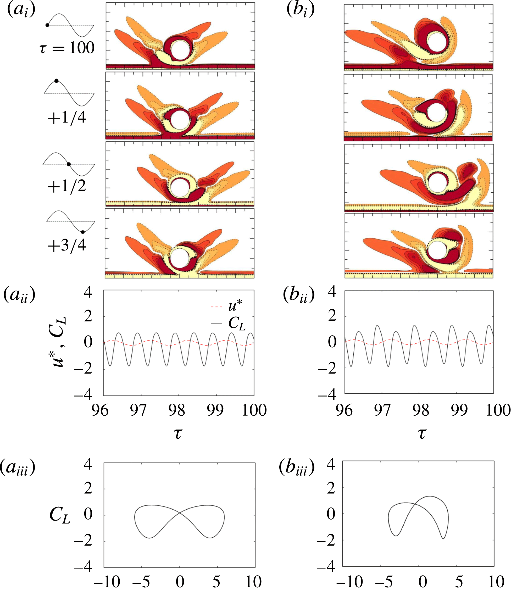
Regime D features V-shaped oblique vortex shedding (figure 9 a) while regime D-A flow exhibits the characteristics of both regimes D and A of an isolated cylinder (figure 9 b). By comparing regimes GVS and D with GVS-A and D-A, two major differences are found: (i) the shed vortices are convected horizontally along the boundary layer in regime GVS/GVS-A while in regime D/D-A they are ejected away with an upwards inclination angle; (ii) the mean lift force in regime GVS/GVS-A is approximately zero and that of regime D/D-A is almost always negative.
Same as figure 7 but (a) regime D at
 $(e/D,KC,\unicode[STIX]{x1D6FD})=(0.5,4,50)$
; and (b) regime A-D at (1, 6, 25).

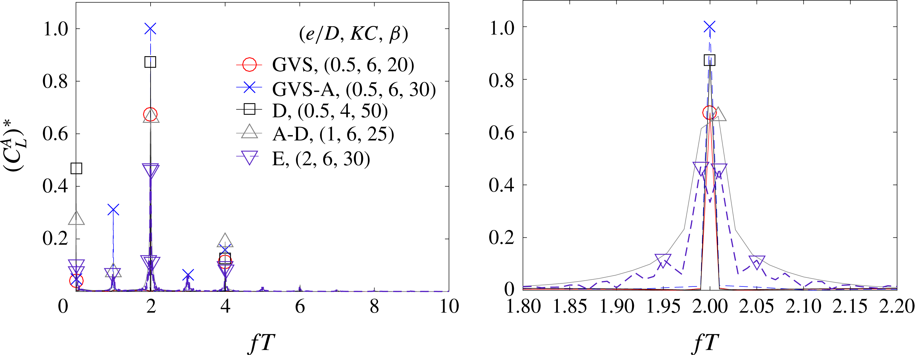
A fast Fourier transform (FFT) of the time series of the lift coefficient in these four regimes is shown in figure 10. The frequency is normalized by the flow oscillation frequency as
 $f/f_{\infty }=fT$
. The amplitude at
 $fT=0$
represents the amplitude of the mean lift force, which is approximately zero for GVS/GVS-A and non-zero for D/D-A. Their primary non-zero frequencies all occur at
 $fT=2$
frequency as expected, and the extra peaks observed at
 $fT=1$
for GVS-A and D-A flows suggest
 $H_{1}$
symmetry breaking.
Comparison of the spectrum of the lift coefficient in regimes GVS, GVS-A, D, D-A and E at the selected parameters as shown in figures 8, 9 and 11 with a close-up view around
 $fT=2$
. The amplitudes
 $(C_{L}^{A})^{\ast }$
have been normalized by the peak value
 $(C_{L}^{A})_{max}=1.41$
from regime GVS-A at
 $fT=2$
.

3.1.3 Regime E
As summarized by Tatsuno & Bearman (Reference Tatsuno and Bearman1990), regime E flow for an isolated cylinder temporarily resembles regime D for the V-shaped transverse vortex street but with intermittent switching of oblique directions with respect to the axis of oscillation. Similar flow patterns are also observed for the wall-bounded cylinder at
 $e/D\geqslant 1$
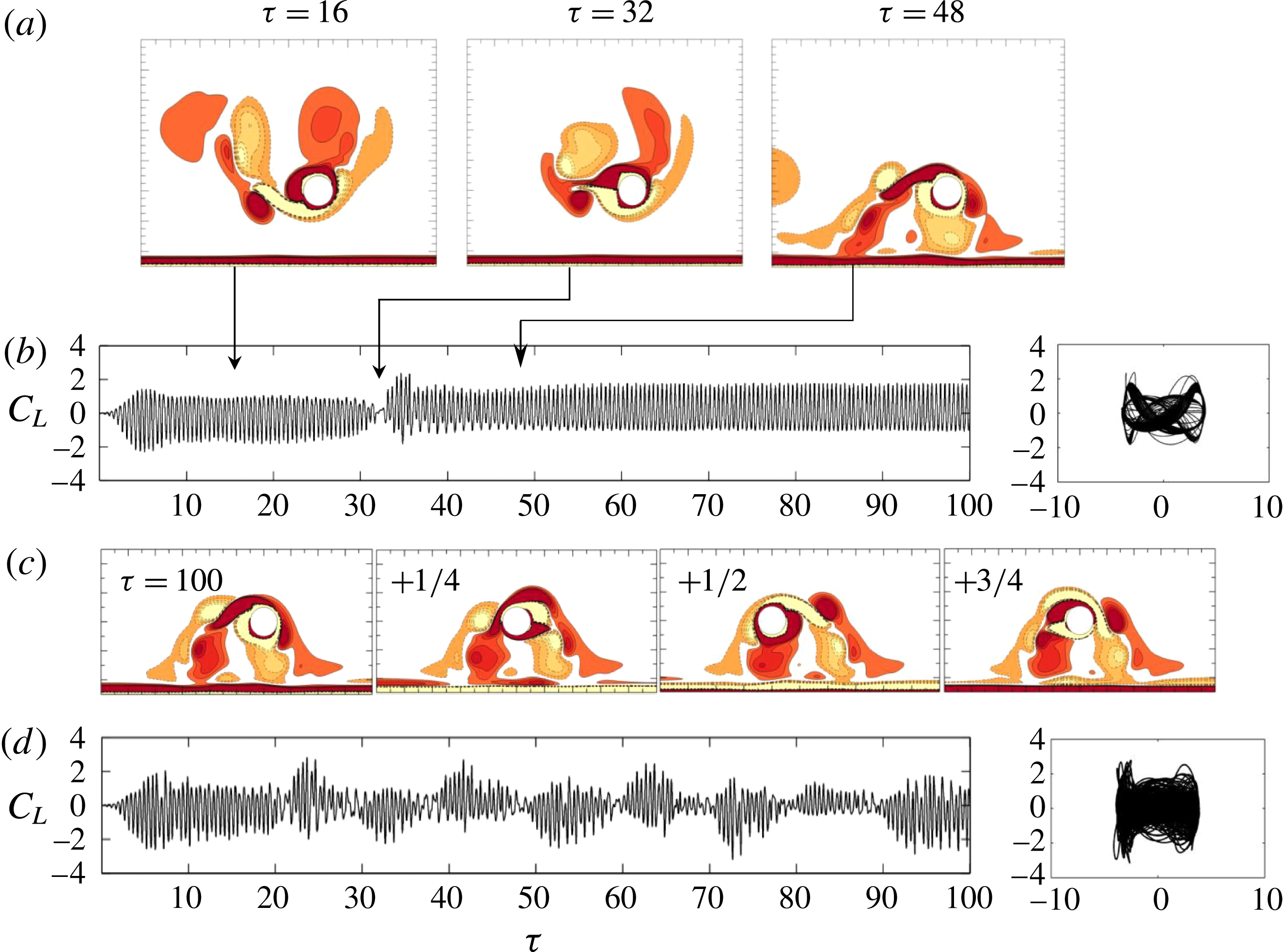
. Figure 11(a) shows an example of regime E flow at
 $(e/D,KC,\unicode[STIX]{x1D6FD})=(2,6,30)$
but with only one switching of the oblique direction at
 $\unicode[STIX]{x1D70F}=32\sim 34$
(the flip of mean lift forces from negative to positive). As shown in figure 10, there are double characteristic frequencies peaking around
 $fT=2$
. Figure 11(b) gives another example with more frequent switching at a higher
 $\unicode[STIX]{x1D6FD}$
value. Correspondingly, the characteristic frequencies still peak around
 $fT=2$
but the FFT results are relatively broad banded. Regime E is not observed at
 $e/D=0.25$
and 0.5, where it is replaced by regimes GVS, GVS-A, D or D-A. Generally, the proximity of a plane boundary appears to have a stabilizing effect on the periodicity of the flow, especially at
 $e/D=0.25$
and 0.5 within
 $Re<300$
. This is partially attributed to the favourable pressure gradient formed over the gap, which will be discussed in § 4. The gap effect is strong at small gap ratios, and dictates the convection direction of vortices.
3.1.4 Regimes
$F^{\prime }$
and F

In regime
 $\text{F}^{\prime }$
, a vortex pair is shed horizontally from the upper surface of the cylinder every half-cycle. An example is shown in figure 12(a). Vortex A shown at
 $\unicode[STIX]{x1D70F}=100$
was developed in the previous flow cycle and forms a vortex pair with the newly generated vortex B at
 $\unicode[STIX]{x1D70F}=100.25$
. This pair of vortices is shed from the cylinder and a new vortex C begins to develop at the end of the first half-cycle of the flow. Since the vortex shedding and development process in the second half of the flow cycle approximately mirror those observed in the first half of the flow cycle, regime
 $\text{F}^{\prime }$
generally possess a
 $H_{1}$
symmetry. Similar flow patterns have also been found in the experimental study of Sumer et al. (Reference Sumer, Jensen and Fredsøe1991) at
 $e/D=0$
and
 $KC=10$
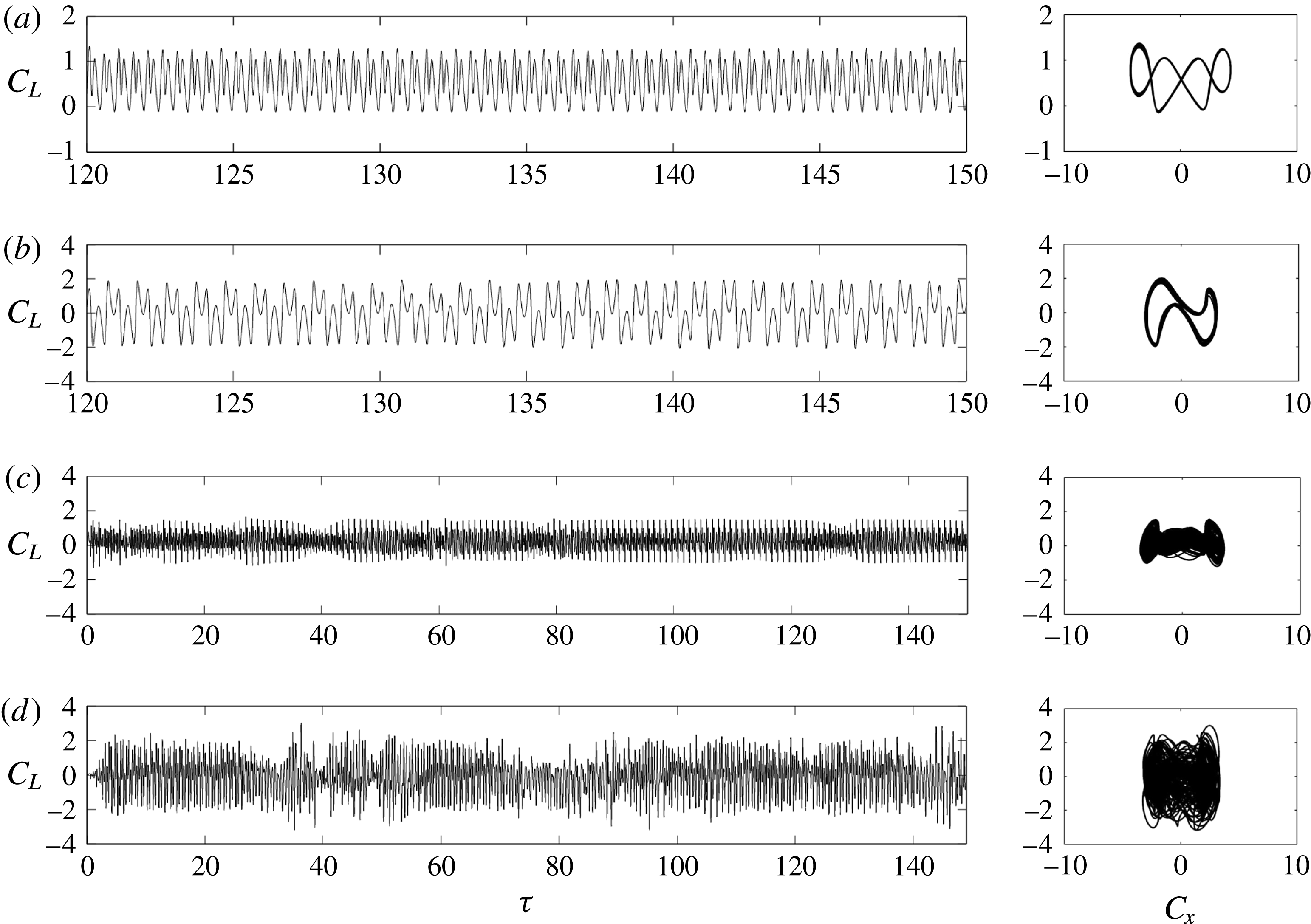
. As shown in figure 13(a), the value of
 $C_{L}$
is almost always positive and is characterized by four peaks every cycle of flow oscillation. The Lissajous phase diagram shows the periodicity and rough
 $H_{1}$
symmetry of the flow.
Regime F flow around a circular cylinder close to a plane boundary is also characterized by diagonal vortex shedding (figure 12
b), similar to its counterpart for an isolated cylinder. However the shed vortices cannot be convected to the far field due to the plane boundary confinement. The cycle-to-cycle variations of the flow are evident in regime F (figure 13
b). A similar observation has also been made by Scandura et al. (Reference Scandura, Armenio and Foti2009) at
 $(e/D,KC,\unicode[STIX]{x1D6FD})=(1.5,10,20)$
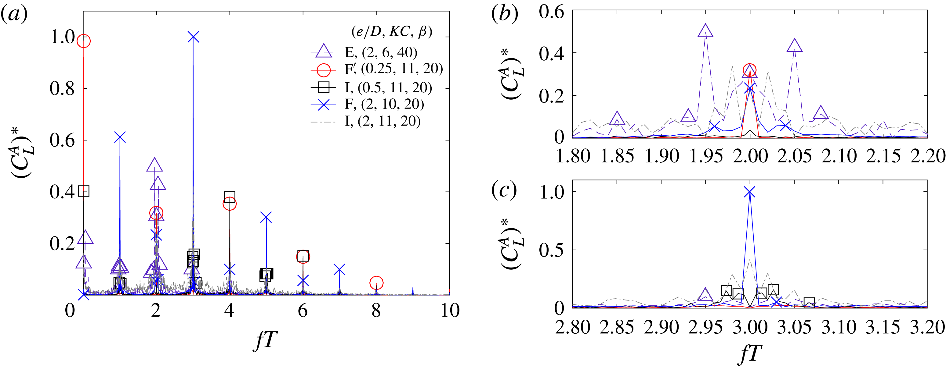
and (0.625, 10, 20). The dominant frequency component of regime
 $\text{F}^{\prime }$
is
 $fT=4$
(figure 14), in contrast to that of regime F at
 $fT=3$
due to the
 $H_{1}$
symmetry breaking in regime F.
(a,c) Instantaneous vorticity contours at different instants and (b,d) the transient trace of
 $C_{L}$
along with the Lissajous phase diagram; (
 $a,b$
) regime E at
 $(e/D,KC,\unicode[STIX]{x1D6FD})=(2,6,30)$
and regime E at (2, 6, 40).

Instantaneous vorticity contours in different flow regimes. The red dot on a scale bar above each contour represents the phase angle of the free oscillatory flow.

Transient trace of
 $C_{L}$
(left) and Lissajous phase diagram of
 $C_{x}{-}C_{L}$
(right) for the same cases as shown in figure 12. (a) Regime
 $\text{F}^{\prime }$
at
 $(e/D,KC,\unicode[STIX]{x1D6FD})=(0.25,11,20)$
; (b) regime F at (2, 10, 20); (c) regime I at = (0.5, 11, 20); and (d) regime I at (2, 11, 20).

Comparison of the spectrum of the lift coefficient in regimes E,
 $\text{F}^{\prime }$
, I and F at the selected parameters as shown in figures 12 and 13 with close-up view around
 $fT=2$
and 3. The amplitudes
 $(C_{L}^{A})^{\ast }$
have been normalized by the peak value
 $(C_{L}^{A})_{max}=1.16$
from regime F at
 $fT=3$
.

The temporal vortex shedding motions of regime
 $\text{F}^{\prime }$
and F in half a cycle are similar to their counterparts in steady flow past a near-wall cylinder (Rao et al.
Reference Rao, Thompson, Leweke and Hourigan2013, Reference Rao, Thompson, Leweke and Hourigan2015). This is possibly because
 $KC/2$
(
 $=U_{m}T/(2D)\sim 5$
) in the oscillatory flow is close to the inverse of the Strouhal number of the steady flow (
 $St=fD/U=D/(UT)\sim 0.2$
) since a vortex pair is shed every half-cycle for the oscillatory flow and every cycle for the steady flow.
3.1.5 Regime I
A regime I flow features irregular and unpredictable cycle-to-cycle variations. Figure 12(c,d) shows two typical examples of flow patterns in regime I at
 $e/D=0.5$
and 2 respectively. The irregular variation of the corresponding transient traces of
 $C_{L}$
indicates the irregularity of both flows (figure 13
c,d). For the first case, it is observed that the pattern of vortex motions is similar to that in regime
 $\text{F}^{\prime }$
in the cycle prior to
 $\unicode[STIX]{x1D70F}=120$
. However, at
 $\unicode[STIX]{x1D70F}=130$
, the flow pattern resembles that in regime HA. Further, at
 $\unicode[STIX]{x1D70F}=140$
and 150, the flow field is characterized by a vortex pair shed from the gap and a single vortex shed from the upper surface. The dominant frequency component of
 $C_{L}$
for regime I is
 $fT=4$
, while multiple peaks occur around
 $fT=3$
as shown in figure 14. This suggests that the flow irregularly switches among several states.
For the second case (figures 12
d and 13
d), the irregularity of the flow is much stronger, and the spectrum of
 $C_{L}$
(figure 14) becomes broadbanded. In the first 30 cycles, the flow is a typical regime F and diagonal vortex shedding is aligned in the south-west and north-east directions. However, the flow becomes unstable and large cycle-to-cycle variations of
 $C_{L}$
are also observed. Although the flow displays the features of regime F sometimes, it also shows irregular transitions, such as those observed at
 $\unicode[STIX]{x1D70F}=42$
and 68 (figures 12
d and 13
d).
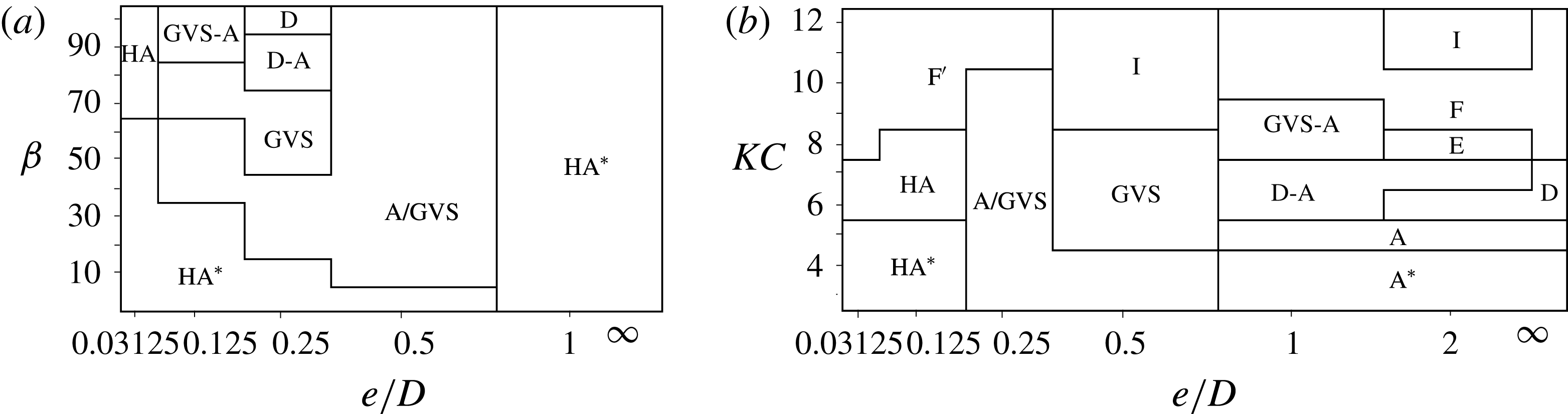
Classifications of the flow regimes at (a)
 $KC=3$
on an
 $e/D$
-
 $\unicode[STIX]{x1D6FD}$
map and (b)
 $\unicode[STIX]{x1D6FD}=20$
on an
 $e/D$
-
 $KC$
map.

The streamwise velocity components
 $u$
at five streamwise locations for different gap ratios at
 $(KC,\unicode[STIX]{x1D6FD})=(5,20)$
at time
 $\unicode[STIX]{x1D70F}=100.25$
. The thickness of Stokes boundary layer by (1.5) is indicated at
 $x/D=10$
.

3.2 Influence of wall proximity
The influence of the plane boundary on flow behaviour is considered in this section. The regime maps shown in figure 5 are re-plotted in figure 15 in the (
 $e/D,\unicode[STIX]{x1D6FD}$
)-space at
 $KC=3$
and in the
 $(e/D,KC)$
-space at
 $\unicode[STIX]{x1D6FD}=20$
, with more data from the two small gap ratios
 $e/D=0.03125$
and 0.125.
The boundaries of regimes
 $\text{HA}^{\ast }/\text{HA}$
are dependent on both
 $e/D$
and
 $\unicode[STIX]{x1D6FD}$
and specifically, depend largely on
 $\unicode[STIX]{x1D6FF}/e$
, where
 $\unicode[STIX]{x1D6FF}$
is inversely proportional to the square-root of
 $\unicode[STIX]{x1D6FD}$
as shown in (1.5) and figure 3. These flows are mostly observed at low
 $\unicode[STIX]{x1D6FD}$
values and small gap ratios. This is expected because the occurrence of H
 $\text{A}^{\ast }$
and HA flows is primarily due to the interaction of the shear layer developed on the gap side of the cylinder surface and the Stokes boundary layer developed on the plane boundary. The shear layers developed on the gap side of the cylinder surface and on the plane boundary are of opposite sign and their interactions become stronger as
 $e/D$
is reduced. This is the primary reason regime H
 $\text{A}^{\ast }$
and HA flows are observed for
 $\unicode[STIX]{x1D6FF}/e\geqslant 1$
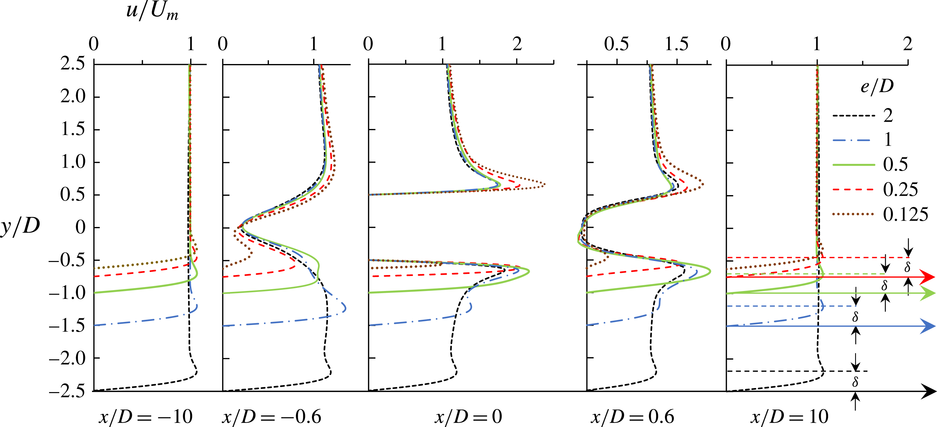
for the gap ratios investigated. This can be further demonstrated by the velocity profiles shown in figure 16, where the streamwise velocity on the gap side around the cylinder is much smaller than that on the top side on the counterpart for larger gap ratios. Similar to regime HA* and HA, regime
 $\text{F}^{\prime }$
only occurs at large
 $\unicode[STIX]{x1D6FF}/e$
where the vortex shedding through the gap is largely suppressed.
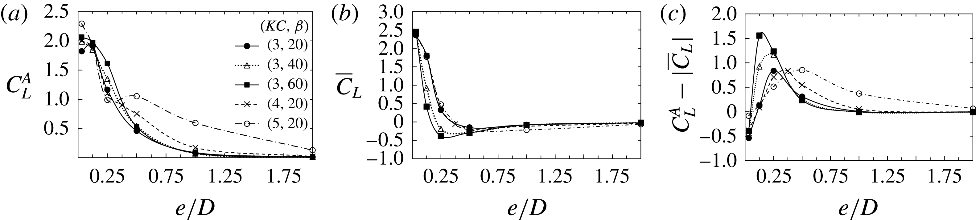
Comparison of the amplitude of the lift coefficient
 $C_{L}^{A}$
at frequency
 $fT=2$
by FFT, the mean lift coefficient
 $\overline{C}_{L}$
, and the difference between
 $C_{L}^{A}$
and
 $|\overline{C}_{L}|$
.

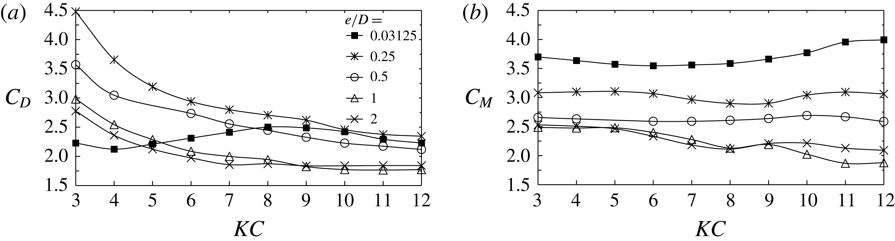
Variation of (a) the drag and (b) the inertia coefficients with
 $KC$
at a fixed stokes number
 $\unicode[STIX]{x1D6FD}=20$
. The drag coefficient
 $C_{D}$
and inertia coefficient
 $C_{M}$
are determined by the Morison equation
 $F_{x}(t)=1/2\unicode[STIX]{x1D70C}DC_{D}|u(t)|u_{\infty }+1/4\unicode[STIX]{x1D70C}D^{2}C_{M}du_{\infty }/dt$
, where
 $\unicode[STIX]{x1D70C}$
is the density of fluid. The least squares method is adopted to determine the coefficients from the inline force over 100 cycles.

As the cylinder is placed further away from the Stokes boundary layer with
 $\unicode[STIX]{x1D6FF}/e<1$
, the influence of the latter becomes weaker and the gap flow is enhanced due to the plane boundary blockage effect (Anagnostopoulos & Minear Reference Anagnostopoulos and Minear2004). This leads to a stronger shear layer on the gap side of the cylinder surface, as shown by the velocity profile for
 $e/D=0.5$
in figure 16. This explains why the regimes GVS/GVS-A appear at
 $\unicode[STIX]{x1D6FF}/e<1$
and
 $e/D\leqslant 1$
. When the gap ratio is further increased, the flow behaviour asymptotically resembles that of an isolated cylinder.
The flow irregularity increases with
 $KC$
and
 $Re$
and is dependent on
 $e/D$
. At
 $e/D=0.25$
, almost no transverse vortex develops within the parameter space and the overall flow pattern is regular. The proximity of the plane boundary stabilizes the flow, especially at
 $KC\leqslant 6$
, because the gap effect is so strong at small gap ratios that it dictates the convection direction of vortices. For intermediate gap ratios, the nonlinear interaction between separated vortices and the Stokes boundary layer gives rise to more irregularity in flow pattern at
 $KC>6$
, compared to the cases that are regarded as regime F for an isolated cylinder. At
 $e/D=2$
, the confinement effect of the plane boundary becomes rather weak and irregularity is more attributed to the vortex shedding pattern around the cylinder itself.
The plane boundary also has a significant influence on the lift coefficient, as shown in figure 17. In general, the lift force is positive (away from the wall) and is largest in regime H
 $\text{A}^{\ast }$
, which occurs at small gap ratios. The mean lift force is approximately zero in regime GVS with relatively strong variation at intermediate gap ratios. The instantaneous lift force vanishes for regime A/
 $\text{A}^{\ast }$
flows. A more careful examination of figure 17 reveals that the amplitude of variation of the lift coefficient (
 $C_{L}^{A}$
) is more sensitive to
 $KC$
, while the mean lift coefficient (
 $|\overline{C}_{L}|$
) is more sensitive to
 $\unicode[STIX]{x1D6FD}$
. Based on the above observation, an index
 $C_{L}^{A}-|\overline{C}_{L}|$
is designed to indicate the strength of gap vortex shedding. At a fixed combination of
 $e/D$
and
 $KC$
, the vortex shedding becomes stronger with increasing
 $\unicode[STIX]{x1D6FD}$
. On the other hand, at a fixed
 $\unicode[STIX]{x1D6FD}$
, the critical
 $e/D$
for the strongest gap vortex shedding increases with
 $KC$
. In addition, the drag and inertia coefficients for
 $\unicode[STIX]{x1D6FD}=20$
are shown in figure 18. Both coefficients increase with decreasing gap ratio, while drag coefficient decreases with increasing
 $KC$
, with an exception at
 $e/D=0.03125$
.
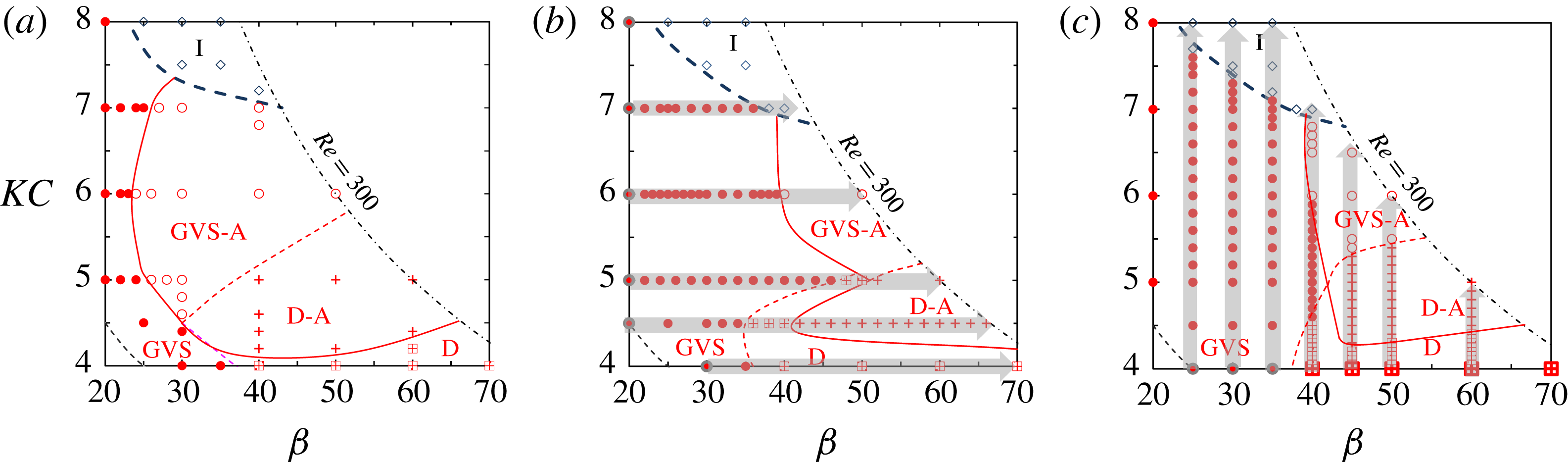
Comparison of the regime map obtained by different initial conditions at
 $e/D=0.5$
. (a) The regime map based on simulations initialized from zero homogeneous condition (same as the figure given in figure 5
b). (b) The regime map based on simulations initialized by a fully developed flow field from the adjacent lower
 $\unicode[STIX]{x1D6FD}$
number. That is, for instance at
 $KC=6$
, the simulation at
 $\unicode[STIX]{x1D6FD}=30$
was started from an instantaneous flow field at
 $\unicode[STIX]{x1D6FD}=29$
. (c) The regime map based on simulations initialized by the fully developed flow from the adjacent smaller
 $KC$
number. The starting point and direction for successive initialization is marked by the dark grey outline and grey arrow, respectively, in (b) and (c).

4 Hysteresis phenomenon
4.1 The influence of initial conditions
Hysteresis, where the flow develops into different flow regimes with different initial conditions, was found for oscillatory flow around a circular cylinder near a plane boundary. To quantify the hysteresis phenomenon, the regime map presented in figure 5 at
 $e/D=0.5$
(obtained with zero initial conditions) is reproduced in figure 19(a), by successively initializing the flow with a fully developed flow field obtained either at the adjacent lower
 $\unicode[STIX]{x1D6FD}$
but constant
 $KC$
, as shown in figure 19(b), or alternatively, at the adjacent lower
 $KC$
but a constant
 $\unicode[STIX]{x1D6FD}$
in figure 19(c). The interval of
 $\unicode[STIX]{x1D6FD}$
or
 $KC$
is not a fixed value and is determined by trial and error, with fine resolutions approaching the regime boundaries. The minimum intervals for
 $KC$
and
 $\unicode[STIX]{x1D6FD}$
used in the simulations are 0.1 and 1, respectively. To facilitate discussions, the zero and non-zero initial conditions (IC) are referred to as zero IC and non-zero IC, respectively.
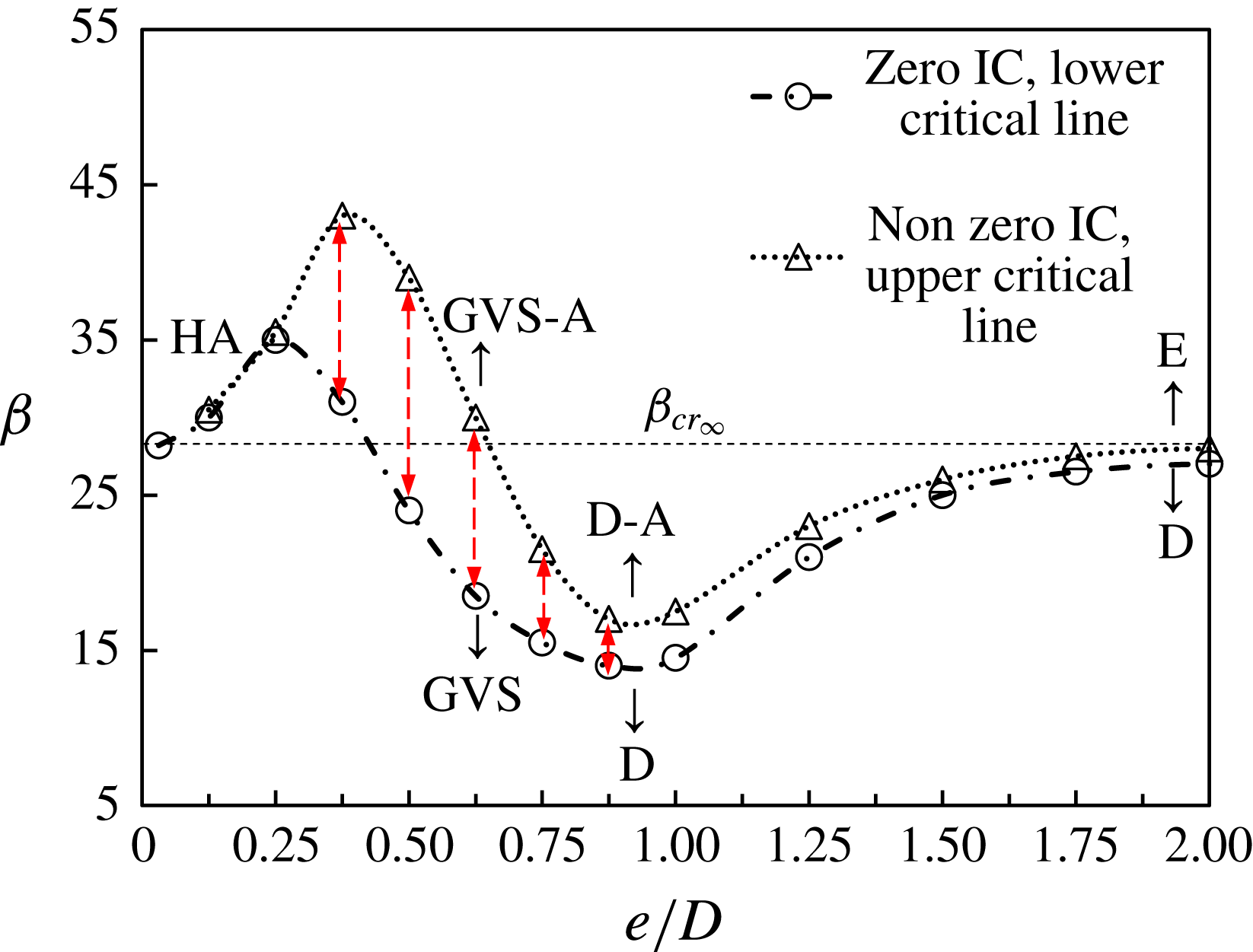
The results shown in figure 19 confirm the existence of hysteresis where the locations of regime boundaries between GVS and GVS-A, D and D-A and GVS-A and D-A are not only dependent on initial conditions but also on the route of parameter change. In the following discussion, the hysteresis phenomenon is illustrated by increasing
 $\unicode[STIX]{x1D6FD}$
at a fixed
 $KC$
only, although other options in changing the parameters are also available.
The marginal curve of the
 $H_{1}$
symmetry at
 $KC=6$
by 2-D Floquet analysis and 2-D DNS with zero initial condition (IC) and non-zero IC. The red dashed lines denote the gap
 $\unicode[STIX]{x0394}\unicode[STIX]{x1D6FD}_{cr}$
between the lower critical Stokes
 $(\unicode[STIX]{x1D6FD}_{cr})_{min}$
and upper critical Stokes number
 $(\unicode[STIX]{x1D6FD}_{cr})_{max}$
.

(a) The variation of Floquet multiplier
 $|\unicode[STIX]{x1D707}|$
for marginal stability of the
 $H_{1}$
symmetry at
 $KC=6$
for an isolated cylinder. The critical Stokes number
 $\unicode[STIX]{x1D6FD}_{cr_{\infty }}=28.3$
is obtained by extrapolating the points with
 $|\unicode[STIX]{x1D707}|>1$
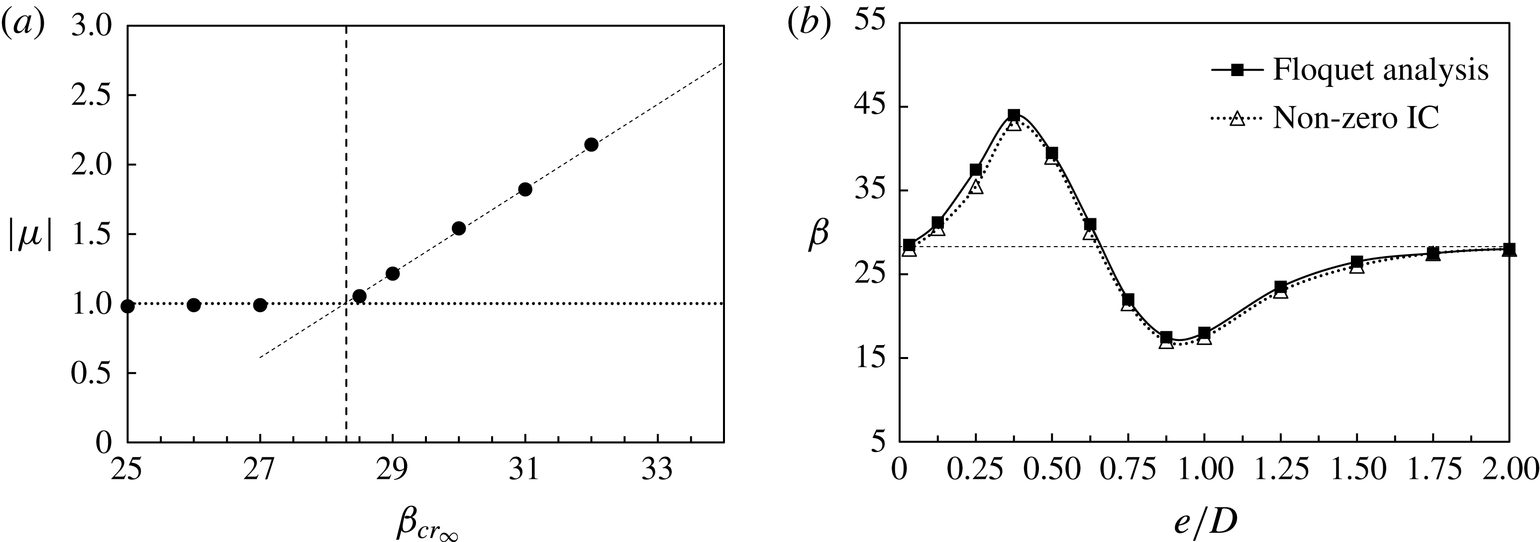
. (b) Comparison on the marginal curves of the
 $H_{1}$
symmetry for
 $0.03125\leqslant e/D\leqslant 2$
at
 $KC=6$
from the Floquet analysis and from 2-D DNS with non-zero initial condition.

It is observed that the regime boundaries obtained using non-zero IC shift to the right (higher
 $\unicode[STIX]{x1D6FD}$
), relative to those obtained using zero IC. For instance, at
 $KC=6$
, the transition from regime GVS to GVS-A occurs at
 $\unicode[STIX]{x1D6FD}=24$
with zero IC (figure 19
a), but does not occur until
 $\unicode[STIX]{x1D6FD}=39.5$
with non-zero IC (figure 19
b). This is attributed to the larger disturbances introduced by zero IC than those by the non-zero IC. For the sets of initial conditions, the base flow in regime GVS with
 $KC=6$
is unconditionally stable with respect to
 $H_{1}$
symmetry for
 $\unicode[STIX]{x1D6FD}<24$
and absolutely unstable for
 $\unicode[STIX]{x1D6FD}>39.5$
. The results demonstrate the subcritical nature of bifurcations of oscillatory flow around a circular cylinder near a plane boundary.
4.2 The influence of gap ratios and boundary conditions
The influence of
 $e/D$
on the hysteresis is also investigated through 2-D DNS in figure 20. Over a range of
 $0.03125\leqslant e/D\leqslant 2.0$
at a fixed
 $KC$
of 6, two marginal stability curves are obtained by initiating the simulations with non-zero IC and zero IC, respectively. The two marginal stability curves are clearly different over
 $0.25<e/D<1.0$
. The one obtained using non-zero IC lies above that obtained using zero IC, and they are referred to as the upper and lower marginal stability curves correspondingly. The gap between these marginal curves is referred to as the hysteresis range between
 $(\unicode[STIX]{x1D6FD}_{cr})_{min}$
and
 $(\unicode[STIX]{x1D6FD}_{cr})_{max}$
, denoted by
 $\unicode[STIX]{x0394}(\unicode[STIX]{x1D6FD}_{cr})=(\unicode[STIX]{x1D6FD}_{cr})_{max}-(\unicode[STIX]{x1D6FD}_{cr})_{min}$
.
Figure 21 further explores the physical mechanisms responsible for the two distinct variation trends through Floquet analysis. The time-stepper approach reported by Barkley & Henderson (Reference Barkley and Henderson1996) is employed in the Floquet analysis. The convergence tolerance for the Floquet multiplier is set as
 $10^{-6}$
. An algorithm for stabilization used to obtain the base flow with enforced
 $H_{1}$
symmetry is detailed in the appendix. The critical Stokes number
 $\unicode[STIX]{x1D6FD}_{cr}$
is estimated by extrapolation of the Floquet multipliers
 $|\unicode[STIX]{x1D707}|$
that are larger than 1.0 to
 $|\unicode[STIX]{x1D707}|$
= 1 as illustrated in figure 21(a), in the same way as that reported in Elston et al. (Reference Elston, Blackburn and Sheridan2006). The marginal stability curve from the Floquet analysis at
 $KC=6$
over a range of
 $e/D$
is shown in figure 21(b), together with that from DNS with non-zero IC. It is seen that the marginal stability curves obtained from the Floquet analysis and DNS agree well. This is attributed to the fact that the infinitesimal disturbances introduced in the Floquet analysis are comparable to the small finite disturbances (less than 1% in terms of overall energy) introduced in DNS with successive initializations. The predicted
 $\unicode[STIX]{x1D6FD}_{cr_{\infty }}$
for an isolated cylinder at
 $KC=6$
is 28.3, and is very close to the value of
 $\unicode[STIX]{x1D6FD}_{cr_{\infty }}\approx 28$
reported by DNS with non-zero IC.
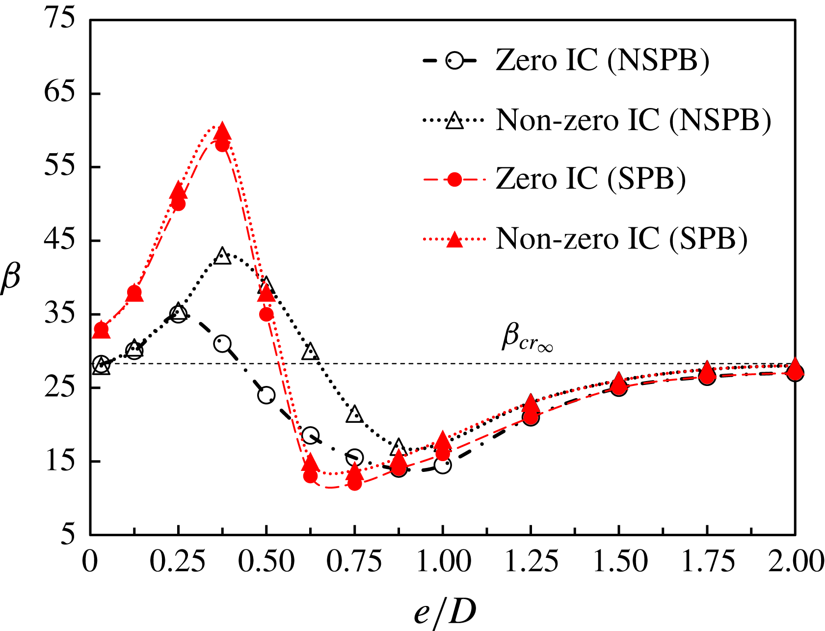
Comparison on the marginal curves of the
 $H_{1}$
symmetry at
 $KC=6$
by DNS with different conditions. NSPB, no-slip plane boundary condition; SPB, slip plane boundary condition; IC, initial condition.

The existence of the no-slip plane boundary possibly affects the stability of the flow through the following two mechanisms. (i) The blockage effect: which introduces a geometric asymmetry about the
 $x$
-axis (
 $y=0$
) and the gap flow; and (ii) the interaction between the Stokes boundary layer developed above the no-slip plane boundary and the shear layers developed over the cylinder surface (along with the resultant shed vortices). Although those two flow mechanisms are prime candidates responsible for the distinct variation trends of
 $\unicode[STIX]{x0394}\unicode[STIX]{x1D6FD}_{cr}$
and
 $\unicode[STIX]{x1D6FD}_{cr}$
observed in this study, their individual roles are not clear. To quantify their individual contributions to the observed trends, additional DNS are carried out with the same parameters except that a slip plane boundary condition (i.e.
 $\unicode[STIX]{x2202}u/\unicode[STIX]{x2202}y=0$
,
 $v=0$
), denoted as SPB, is imposed on the plane boundary. Under SPB, the influence of the Stokes boundary layer is removed while the blockage effect is retained. The marginal stability curves obtained for oscillatory flow above an SPB through DNS with zero IC and non-zero IC are shown in figure 22, together with their counterparts from the no-slip plane boundary (NSPB). It is seen that the overall variation trends of the marginal stability curves with
 $e/D$
obtained using an SPB are similar, but the hysteresis range
 $\unicode[STIX]{x0394}\unicode[STIX]{x1D6FD}_{cr}$
for flow above an SPB is much smaller than its counterpart above a NSPB and remains almost a constant over the entire range of
 $e/D$
. This suggests that the existence of the Stokes boundary layer over the plane boundary is mainly responsible for the large values of
 $\unicode[STIX]{x0394}\unicode[STIX]{x1D6FD}_{cr}$
over
 $0.25<e/D<1$
, possibly through the interaction between the Stokes boundary layer and the shear layers developed over the cylinder. This is indirectly supported by the fact that
 $\unicode[STIX]{x0394}\unicode[STIX]{x1D6FD}_{cr}$
values obtained using the two sets of boundary conditions are almost identical for
 $e/D>1.0$
, where the interaction is expected to be weak. The interaction between the Stokes boundary layer and the flow developed around the cylinder is illustrated qualitatively in figure 23 for
 $0.125\leqslant e/D\leqslant 1.0$
, in comparison with the flow around the cylinder over an SPB in the same range of
 $e/D$
.
The variation of
 $\unicode[STIX]{x1D6FD}_{cr}$
with
 $e/D$
for the case with a NSPB (shown in figure 20) is also explained. The observed decrease of
 $\unicode[STIX]{x1D6FD}_{cr}$
with
 $e/D$
over
 $0.875\leqslant e/D<2.0$
is due to peak flow velocity increase through the gap, induced by the blockage effect of the plane boundary. The flow instability over the range of
 $e/D$
is expected to be dominated by the flow around the gap side. Therefore, as the cylinder moves closer to the plane boundary, the blockage effect keeps increasing, leading to a further reduction of
 $\unicode[STIX]{x1D6FD}_{cr}$
from
 $\unicode[STIX]{x1D6FD}_{cr_{\infty }}$
. The increase of peak flow velocity through the gap with reduction in
 $e/D$
is quantified in figure 16 (
 $x/D=0$
) till
 $e/D=0.5$
, although it is sampled at a fixed point. It is also seen the peak velocity over the top of the cylinder barely changes. The observed trend in peak velocity is expected to be typical for the (
 $KC,\unicode[STIX]{x1D6FD}$
)-space. When
 $e/D$
is reduced below a critical value (about 0.875),
 $\unicode[STIX]{x1D6FD}_{cr}$
starts to increase with reduction in
 $e/D$
, peaking at
 $e/D=0.25$
for zero IC and 0.375 for non-zero IC.
Comparison of instantaneous contours of
 $\unicode[STIX]{x1D714}_{z}$
between slip plane boundary condition (SPB, upper) and no-slip boundary condition (NSPB, lower).

4.3 The favourable pressure gradient
The observed variation of
 $\unicode[STIX]{x1D6FD}_{cr}$
with
 $e/D$
over
 $0.375\leqslant e/D<0.873$
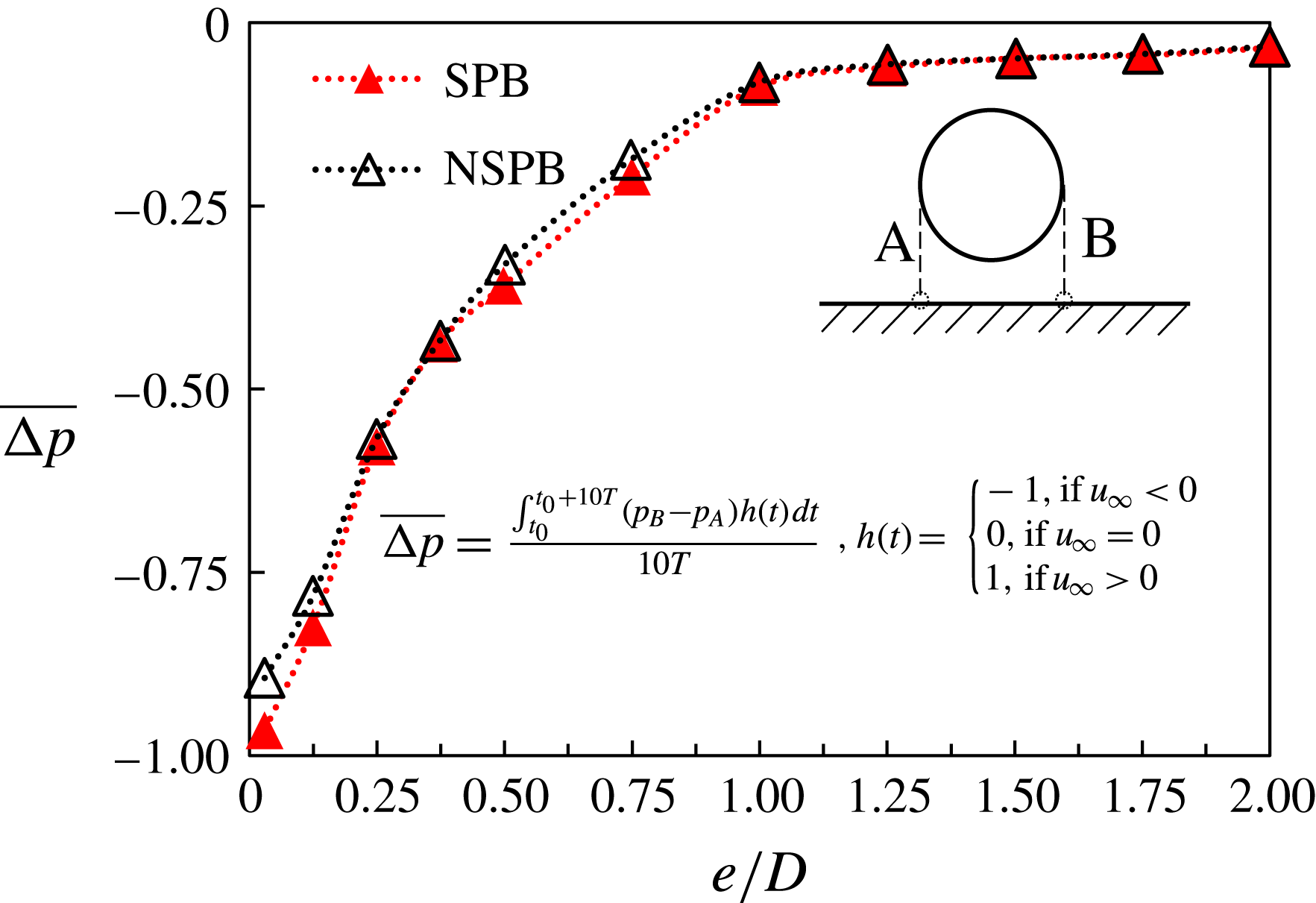
is attributed to the stabilization introduced by the favourable pressure gradient over the gap. The favourable pressure gradient over the gap increases as
 $e/D$
is reduced, as shown in figure 24 where the variation of pressure gradient over two points on the plane boundary with
 $e/D$
is quantified at
 $(KC,\unicode[STIX]{x1D6FD})=(6,30)$
. It is well known from stability theory that a favourable pressure gradient often improves the stability of the flow. Therefore, the effect of the favourable pressure gradient on the flow around the gap side of the cylinder is to improve its stability, counter-balancing the effect of the peak flow velocity increase mentioned above. The lower peak of
 $\unicode[STIX]{x1D6FD}_{cr}$
near
 $e/D=0.875$
signals the onset of the effect of favourable pressure gradient. As
 $e/D$
is further reduced, the increase in peak velocity through the gap starts to diminish while the favourable pressure gradient starts to increase rapidly, causing a change of flow instability from occurring on the gap side to the top side of the cylinder, at a gap ratio where
 $\unicode[STIX]{x1D6FD}_{cr}$
peaks at
 $(e/D)_{\mathit{peak}}=0.25$
and 0.375 for zero IC and non-zero IC, respectively. The reduction of
 $\unicode[STIX]{x1D6FD}_{cr}$
with
 $e/D$
for
 $e/D<(e/D)_{peak}$
is because the flow over the dominant side (the top side) for flow instability is enhanced as
 $e/D$
is reduced. The peak velocity above the cylinder increases with reduction of
 $e/D$
for
 $e/D<(e/D)_{peak}$
as shown in figure 16 (
 $x/D=0$
).
4.4 Eigenmodes by linear stability analysis
Figure 25 illustrates the influence of wall proximity on the eigenmodes. It is seen that the leading eigenmodes are scattered around the gap side of the cylinder for
 $e/D>0.25$
and over the top side for
 $e/D<0.25$
. The transition of the initiation location of flow instability thus takes place at
 $e/D=0.25$
. This is consistent with the trends of marginal stability curves obtained by DNS shown in figure 22.
Variation of pressure drop between the detecting points A and B as a function of gap ratios at
 $KC=6$
and
 $\unicode[STIX]{x1D6FD}=30$
.

4.5 Discussion on the marginal stability curves
The flow mechanisms responsible for the differences between the marginal stability curves obtained using a NSPB and an SPB are explained based on the above results. Three major differences between the marginal stability curves obtained using a NSPB and an SPB are observed in figure 22: (i) the marginal stability curves obtained using an SPB shift slightly to the left of those obtained using a NSPB; (ii) the difference between the maximum
 $(\unicode[STIX]{x1D6FD}_{cr})_{max}$
and the minimum
 $(\unicode[STIX]{x1D6FD}_{cr})_{min}$
for using an SPB is larger than its counterpart obtained using a NSPB; and (iii) the observed difference in
 $\unicode[STIX]{x1D6FD}_{cr}$
values at
 $e/D=0.03125$
. These differences can all be attributed to the existence of the Stokes layer for a NSPB and the absence of the Stokes layer for an SPB. The absence of the Stokes layer for an SPB causes an increase of flow rate through the gap side in the case with a NSPB at the same gap ratio, resulting in a smaller gap ratio that is required to pass the same gap flow. This causes the marginal stability curves obtained using an SPB to shift to the left of those obtained using a NSPB. The increased flow rate through the gap for an SPB also leads to a smaller
 $(\unicode[STIX]{x1D6FD}_{cr})_{min}$
and a larger
 $(\unicode[STIX]{x1D6FD}_{cr})_{max}$
than their counterparts for a NSPB. The difference in
 $\unicode[STIX]{x1D6FD}_{cr}$
values at
 $e/D=0.03125$
is because the gap still has considerable influence on
 $\unicode[STIX]{x1D6FD}_{cr}$
even at such a small gap size for an SPB while such an influence is diminished for a NSPB due to the influence of the Stokes boundary layer.
5 Flow three-dimensionality considerations
The findings reported so far in this study are purely based on 2-D DNS and 2-D Floquet analysis. A legitimate question about the validity of the findings is the influence of three-dimensionality on the findings presented in this study, as the flow will be three-dimensional over a certain area of the parameter space.
For an isolated cylinder, previous studies have demonstrated that 2-D simulations are capable of resolving the flow regimes accurately in the parameter space (Nehari et al.
Reference Nehari, Armenio and Ballio2004; Elston et al.
Reference Elston, Blackburn and Sheridan2006; Tong et al.
Reference Tong, Cheng, Xiong, Draper, An and Lou2017). Therefore the question comes down to whether the existence of the plane boundary will enhance the three-dimensionality of the flow to such a degree that 2-D models are no longer able to simulate the key features of the flow. As suggested by Scandura et al. (Reference Scandura, Armenio and Foti2009), flow three-dimensionality tends to be suppressed as the cylinder approaches the wall and the results of 3-D simulations are similar to 2-D results at
 $Re=200$
. For a time-periodic flow, the 3-D effects only modulate the sectional transverse force along the axis of the cylinder, but rarely modify the overall force on the cylinder. Based on the results presented in figure 22, the flow three-dimensionality is expected to be enhanced as compared to that around an isolated cylinder when
 $e/D$
is reduced down to around 0.5 and weakened for
 $e/D<0.5$
. The enhancement of three-dimensionality is mainly on the gap side due to the increase in peak flow velocity caused by the blockage effect. Since the magnitude of velocity increase on the gap side is rather insignificant (figure 16), its influence on flow three-dimensionality is expected to be small. For this reason, it is believed that the present findings will remain valid when the flow becomes three-dimensional over a certain area of the parameter space. To demonstrate this, 3-D DNS and 3-D Floquet analysis are carried out for a few cases only, due to the limited computational resources.
Instantaneous contours
 $\unicode[STIX]{x1D714}_{z}$
of the base flow (grey lines) and the leading eigenmode (colour contours) at
 $KC=6$
and a
 $\unicode[STIX]{x1D6FD}$
just above
 $\unicode[STIX]{x1D6FD}_{cr}$
with respect to
 $H_{1}$
symmetry at different gap ratios.

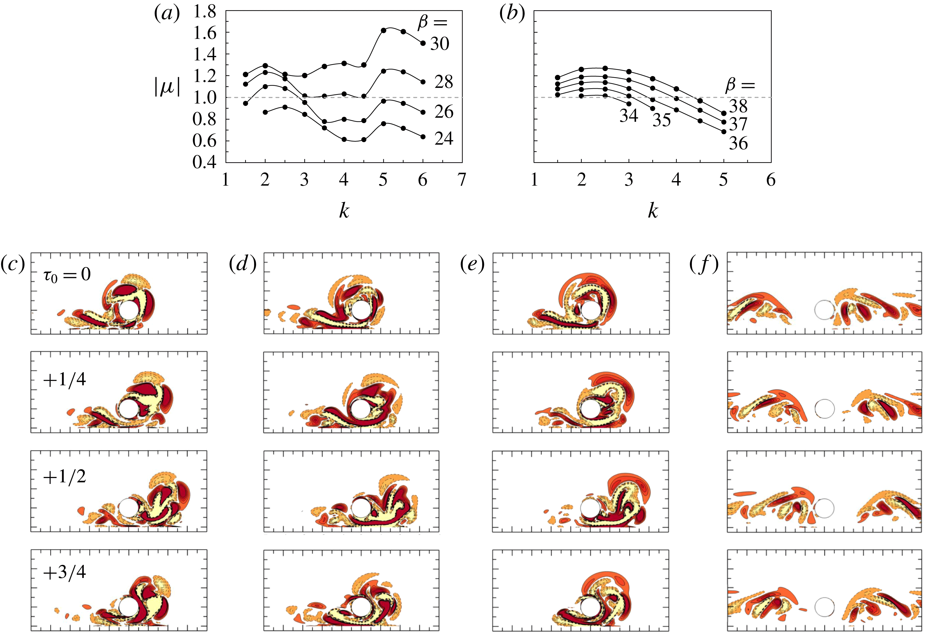
Floquet multipliers as functions of wavenumber and Stokes number for the three-dimensional instability at
 $(e/D,KC)=(0.5,6)$
are shown in (a) for regime GVS-A, whose base flows are obtained from zero IC, and (b) for regime GVS, whose base flows are obtained from non-zero IC. The critical wavenumber (k) and Stokes number are estimated at (a)
 $k_{c}=2.2$
and
 $\unicode[STIX]{x1D6FD}_{cr,3-\text{D}}=24.8$
, (b)
 $k_{c}=2.3$
and
 $\unicode[STIX]{x1D6FD}_{cr,3-\text{D}}=33.9$
. The vorticity contours of eigenmodes at
 $k=2$
, 4 and 5.5 and
 $\unicode[STIX]{x1D6FD}=26$
for GVS-A are shown in (
 $c$
–
 $e$
), and those at
 $k=2.5$
and
 $\unicode[STIX]{x1D6FD}=34$
for GVS are shown in (f), respectively.

5.1 Three-dimensional Floquet stability analysis
Three-dimensional Floquet stability analysis is conducted at
 $(e/D,KC)=(0.5,6)$
, following the same approach of Henderson & Barkley (Reference Henderson and Barkley1996) and Elston et al. (Reference Elston, Blackburn and Sheridan2006). The purpose of 3-D Floquet stability analysis is mainly to provide guidance to 3-D DNS in determining the critical Stokes number for onset of the 3-D instability, and the spanwise length of the computational domain through determining the spanwise wave length of the 3-D instability. The Floquet analysis results are shown in figure 26(a,b), where the base flows are obtained using zero IC and non-zero IC (by increasing
 $\unicode[STIX]{x1D6FD}$
), respectively. The fully developed base flow initialized with zero IC is in GVS-A while that initialized with non-zero IC evolves into a GVS flow. The critical Stokes number for the 3-D instability for the regime GVS-A base flow is
 $\unicode[STIX]{x1D6FD}_{cr,\text{3-D}}=24.8$
and for the GVS base flow is
 $\unicode[STIX]{x1D6FD}_{cr,\text{3-D}}=33.9$
. This indicates that the flow would remain two-dimensional up to
 $\unicode[STIX]{x1D6FD}=24.8$
with zero IC and
 $\unicode[STIX]{x1D6FD}=33.9$
with non-zero IC. For
 $24<\unicode[STIX]{x1D6FD}_{cr,\text{3-D}}=33.9<39.5$
(where
 $\unicode[STIX]{x1D6FD}=24$
and 39.5 denote the lower and upper
 $\unicode[STIX]{x1D6FD}_{cr}$
for 2-D
 $H_{1}$
symmetry breaking), there must exist a range of
 $\unicode[STIX]{x1D6FD}$
where 3-D instability is not involved in the hysteresis phenomenon. However, whether the upper
 $\unicode[STIX]{x1D6FD}_{cr}$
for 2-D
 $H_{1}$
symmetry breaking is affected by 3-D instability remains to be checked by fully 3-D simulations.
5.2 Three-dimensional DNS
The purpose of 3-D DNS is to confirm the credibility of the hysteresis results and regime maps that are identified by 2-D simulations, especially for the flow in regime GVS. A convergence test on the choice of spanwise length
 $L_{z}$
and resolution
 $2N$
in the 3-D DNS is carried out at
 $e/D=0.5$
with
 $\unicode[STIX]{x1D6FD}=30$
and
 $KC=6$
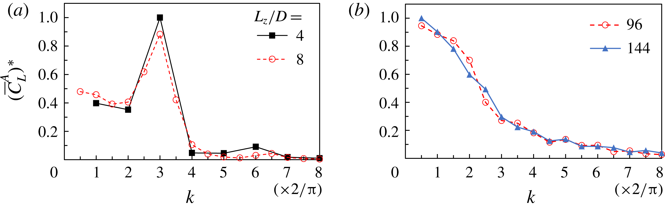
and the results are shown in figure 27. Figure 27(a) shows that for both
 $L_{z}/D=4$
and 8 the primary wavenumber is
 $2k/\unicode[STIX]{x03C0}$
= 3, despite the lowest wavenumber extending to
 $2k/\unicode[STIX]{x03C0}=0.5$
for
 $L_{z}/D=8$
. Therefore, a conservative selection of
 $L_{z}/D=8$
is made to allow for a wider spectrum being included. The spanwise resolution is further checked at maximum Reynolds number (
 $Re=300$
, or
 $\unicode[STIX]{x1D6FD}=50$
). Different from that at
 $\unicode[STIX]{x1D6FD}=30$
, the amplitude of the lift force monotonically decreases at higher wavenumber, which is different from the case of
 $\unicode[STIX]{x1D6FD}=30$
, but similar to the case reported by Scandura et al. (Reference Scandura, Armenio and Foti2009). Since the results obtained with
 $2N=96$
and 144 are very similar,
 $2N=96$
is chosen to allow for a timely completion of the 3-D simulations up to
 $Re=300$
.
Comparison of characteristic wavenumber obtained by FFT of the sectional lift force at (a)
 $\unicode[STIX]{x1D6FD}=30$
for spanwise length
 $L_{z}/D=4$
and 8 with fixed
 $2N=96$
, and (b)
 $\unicode[STIX]{x1D6FD}=50$
for spanwise resolution
 $2N=96$
and 144 with fixed
 $L_{z}/D=8$
. Results are averaged for 10 oscillation periods from
 $\unicode[STIX]{x1D70F}=50$
to 60 when the three-dimensional instabilities have been well developed. The original wavenumber is normalized by
 $2\unicode[STIX]{x03C0}/L_{z}$
for comparison of different spanwise length. The amplitudes
 $(\overline{C}_{L}^{A})^{\ast }$
have been normalized by the peak value.

Figure 28 shows results of 3-D DNS between
 $\unicode[STIX]{x1D6FD}=30$
and 50 with
 $(e/D,KC)=(0.5,6)$
, visualized by using the
 $Q$
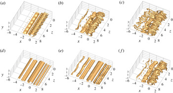
-criterion (Hussain Reference Hussain1986). Based on the 2-D regime maps shown in figure 19(a), the fully developed flows initiated with zero IC are in regime GVS-A. Although the corresponding 3-D results shown in figure 28(a–c) clearly indicate that the flows are 3-D at
 $\unicode[STIX]{x1D6FD}=30$
, 40 and 50, their structures resemble 2-D regime GVS-A structures, and are also similar to the 3-D structures shown in figure 20 of Scandura et al. (Reference Scandura, Armenio and Foti2009) at
 $(e/D,KC,\unicode[STIX]{x1D6FD})=(0.625,10,20)$
. If the spanwise-averaged flow is used to classify the flow, the flows at
 $\unicode[STIX]{x1D6FD}=30$
, 40 and 50 will be categorized in regime GVS-A.
Figure 29 compares the spanwise-averaged flow and corresponding trace of force coefficients of 3-D results with those obtained using 2-D simulation at
 $\unicode[STIX]{x1D6FD}=50$
, where the three-dimensionality is strongest among the three cases examined. There is no significant difference between them, suggesting that similar flow regime maps to those obtained using 2-D simulations (figure 19
a) would have been obtained if 3-D DNS were employed. In addition, the hysteresis is also observed in the 3-D DNS, as shown in figure 28(d) where the flow remains in regime GVS and two-dimensional at
 $\unicode[STIX]{x1D6FD}=30$
when it is initiated with non-zero IC. Figure 28(e) shows that the flow is weakly three-dimensional at
 $\unicode[STIX]{x1D6FD}=38$
but maintains the features of regime GVS. The obvious regime GVS-A is observed at
 $\unicode[STIX]{x1D6FD}=40$
in figure 28(f) with non-zero IC, indicating the upper limit for
 $H_{1}$
symmetry breaking is consistent with
 $\unicode[STIX]{x1D6FD}_{cr}=39.5$
predicted by the 2-D model. This gives us confidence that although the regime maps and hysteresis range obtained using 2-D simulation may not be the exactly same as those obtained using 3-D simulations, 2-D results do reflect the real flow mechanisms well.
The isosurface of
 $Q=0.25$
of the 3-D DNS results at
 $(e/D,KC)=(0.5,6)$
: GVS-A flow at (a)
 $\unicode[STIX]{x1D6FD}=30$
, (b) 40 and (c) 50 by zero IC; and GVS flow at (c)
 $\unicode[STIX]{x1D6FD}=30$
, (d) 38 and (f) 40 by successive iteration.

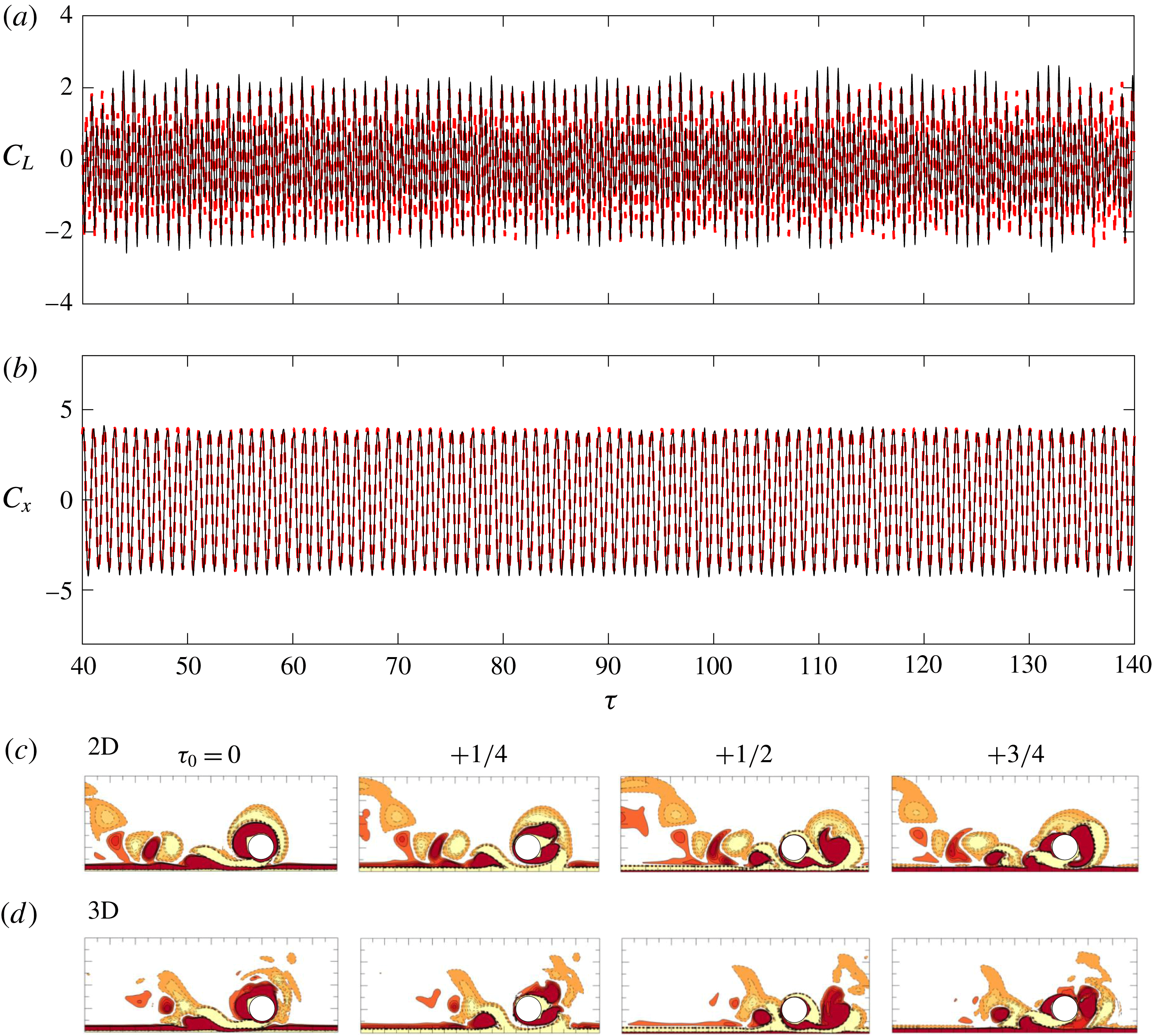
Comparison of (a) lift force coefficient and (b) inline force coefficient between 3-D (- - - - - red) and 2-D (——) results, and corresponding instantaneous vorticity contours (c) and (d) at
 $(e/D,KC,\unicode[STIX]{x1D6FD})=(0.5,6,50)$
. The 3-D results are averaged along the spanwise direction.

6 Conclusions
Oscillatory flow around a circular cylinder close to a plane boundary at low-to-intermediate
 $KC$
(
 $3\leqslant KC\leqslant 12$
) and
 $Re$
(
 ${\leqslant}300$
) is studied by both direct numerical simulation (DNS) and Floquet analysis. The main conclusions are summarized as follows.
(i) In total twelve flow regimes are classified and mapped out at four gap-to-diameter ratios (
 $e/D=0.25$
, 0.5, 1 and 2). Some of the flow regimes are unique for the flow investigated.
(ii) The influence of the plane boundary on the flow regimes is discussed, in terms of the size of the gap (e) and the thickness of the Stokes boundary layer (
 $\unicode[STIX]{x1D6FF}$
). At relatively large
 $\unicode[STIX]{x1D6FF}/e$
(
 ${>}1.0$
) values, regime
 $\text{HA}^{\ast }$
, HA and
 $\text{F}^{\prime }$
appear when the vortices only develop on the top side of the cylinder because of the suppression of vortex shedding through the gap. At
 $e/D\leqslant 1$
and
 $\unicode[STIX]{x1D6FF}/e<1.0$
, the plane boundary restricts the formation of transverse vortices but enhances the flow through the gap with horizontal vortex shedding along the streamwise direction, giving rise to regime GVS (gap vortex shedding) and GVS-A. As
 $e/D$
increases beyond
 $e/D>1.0$
, the influence of the plane boundary becomes weak and the flow asymptotes towards that around an isolated circular cylinder.
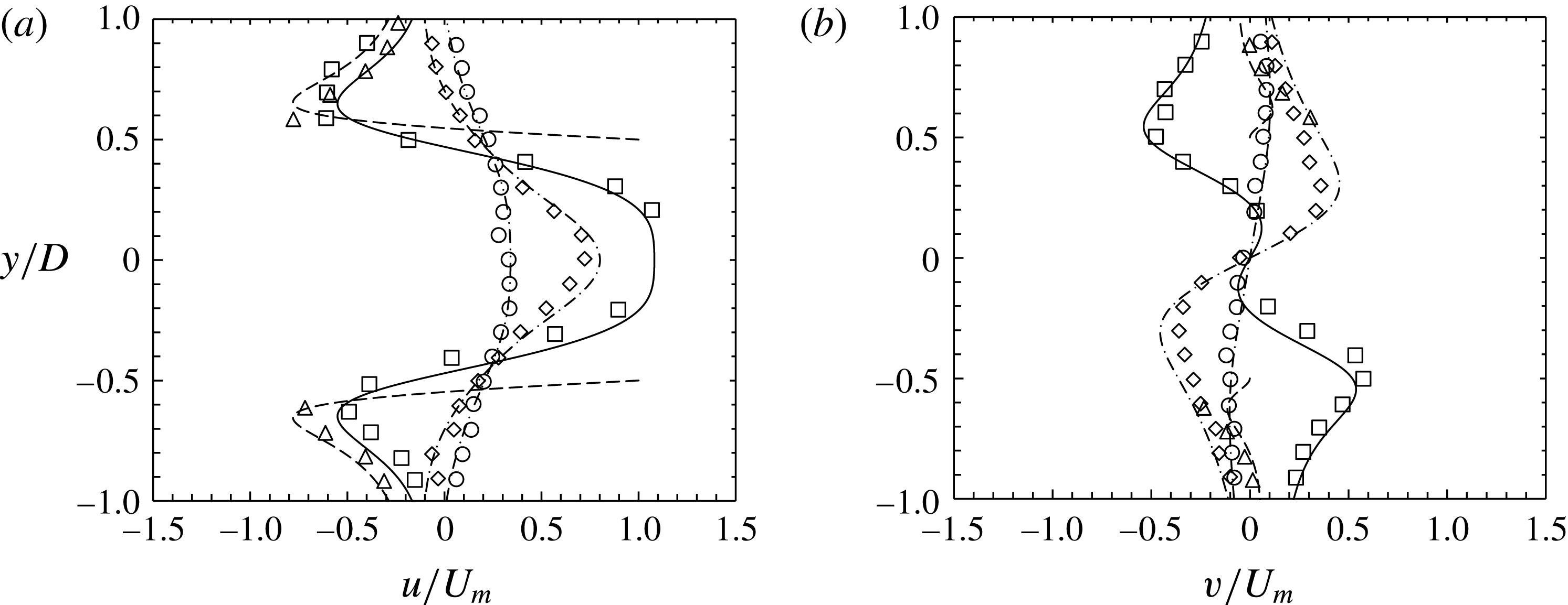
Comparison of the streamwise and transverse velocity distribution of an isolated cylinder for
 $(KC,\unicode[STIX]{x1D6FD})=(5,20)$
between the present results (lines) and the experimental data (markers) by Dütsch et al. (Reference Dütsch, Durst, Becker and Lienhart1998). Due to the difference between oscillatory flow around fixed cylinder (present study) and oscillating cylinder in otherwise still water, the phase angle and velocity were transformed through:
 $\unicode[STIX]{x1D6F9}=\unicode[STIX]{x1D711}-90^{\circ }$
,
 $u=U(t)-U_{m}\text{sin}(\unicode[STIX]{x1D711})$
and
 $v=V(t)$
, where
 $\unicode[STIX]{x1D6F9},U$
and
 $V$
are the parameters in the present study, and
 $\unicode[STIX]{x1D719},u$
and
 $v$
are the ones in Dütsch et al. (Reference Dütsch, Durst, Becker and Lienhart1998), and
 $U_{m}$
is the maximum free-stream velocity. The velocity components were sampled at
 $x/D=0.6$
, ▫/——; 0.0, ▵/; 0.6, ♢/–
 $\cdot$
–
 $\cdot$
; 1.2, ○/— ⋅ ⋅ —.

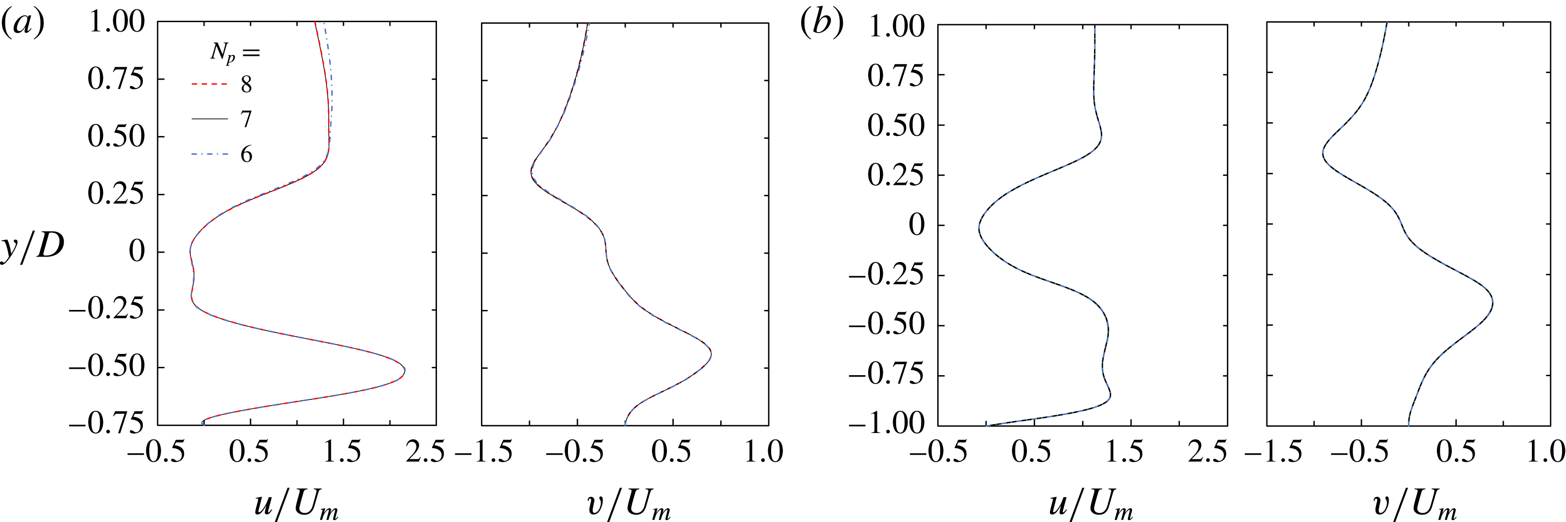
 $N_{p}$
-convergence results for the velocity components
 $u$
and
 $v$
at
 $x=0.6D$
and
 $\unicode[STIX]{x1D70F}=100.25$
, using parameter values of (a)
 $(e/D,KC,\unicode[STIX]{x1D6FD})=(0.5,3,100)$
and (b) (0.25, 3, 100).

(iii) Hysteresis is discovered over a relatively large range
 $0.25<e/D<1$
. Additional direct numerical simulations with a slip plane boundary demonstrate that the Stokes boundary layer is responsible for the large hysteresis range.
(iv) The blockage effect due to the plane boundary, the favourable pressure gradient over the gap between the cylinder and the plane boundary and the side swapping of the locations where flow instability occurs (relative to the cylinder) are all responsible for the trend in the marginal stability curve for a tempo-spatial symmetry with
 $e/D$
.
(v) Three-dimensionality has little influence on the hysteresis effect and the 2-D
 $H_{1}$
symmetry breaking over the parameter space covered in this study. The spanwise-averaged vortex motions of the 3-D flow are not very different from those obtained by the 2-D simulation. The regime classification based on the 2-D results is largely correct and reflects the physics of the flow.
Acknowledgements
C.X. would like to express his sincere thanks to the University of Western Australia for the SIRF Scholarship provided to support this study. L.C. would like to acknowledge the support from the National Natural Science Foundation of China (Grants ID 51479025). H.A. would like to acknowledge the support by the Australian Research Council through DECRA Scheme (DE150100428). The authors would like to acknowledge the support from the Pawsey Supercomputing Centre with funding from the Australian Government and the Government of Western Australia.
Supplementary movies
Supplementary movies are available at https://doi.org/10.1017/jfm.2018.164.
Appendix A. Model validation
The predicted velocity distributions around an isolated cylinder are validated against the experimental data of Dütsch et al. (Reference Dütsch, Durst, Becker and Lienhart1998) in figure 30. The coordinate system of the present data was transformed into those used in Dütsch et al. (Reference Dütsch, Durst, Becker and Lienhart1998) (see caption), where the cylinder oscillated in otherwise still water. The comparison suggests that the numerical results agree well with the measured data.
Validation of Floquet analysis on the instantaneous vorticity contours for isolated cylinder against Elston et al. (Reference Elston, Blackburn and Sheridan2006): (a) the real and imaginary parts of the Floquet eigenfunction at the same phase of the motion cycle between results from present study (colour) and Elston et al. (Reference Elston, Blackburn and Sheridan2006) (grey) at
 $KC=4.7$
and
 $\unicode[STIX]{x1D6FD}=40$
; (b) streamwise vorticity isosurface for the regime D instability at
 $(KC,\unicode[STIX]{x1D6FD},k)=(7,14.15,1.75)$
, Elston et al. (Reference Elston, Blackburn and Sheridan2006) (left) and present study (right); (c) comparison of the curve of marginal stability from two-dimensional Floquet analysis. (d) Floquet multipliers as functions of wavenumber
 $k$
for the three-dimensional secondary instability of regime D at
 $(KC,\unicode[STIX]{x1D6FD})=(8,10.85)$
. The figures are reproduced with the permission of the authors.

Flow diagram for demonstration of the stabilization technique to obtain the
 $H_{1}$
symmetric flow.

The transient trace of
 $C_{L}$
for the isolated cylinder at
 $KC=6$
: (a) and (b) by non-zero initial condition, indicating
 $28<\unicode[STIX]{x1D6FD}_{cr_{\infty }}<29$
, (c) and (d) by zero initial condition at
 $\unicode[STIX]{x1D6FD}=28.5$
, where the latter is obtained with stabilization technique for Floquet analysis. The dashed line in (d) denotes the trace of
 $C_{L}$
of
 $0.5<t_{0}\leqslant 1$
is the repetition of that of
 $0<t_{0}\leqslant 0.5$
when using the stabilization technique.

The domain size effect is investigated on a family of meshes, which are all similar to figure 4(b) except for different resolutions employed below the cylinder at different gap ratios. It was performed at the maximum
 $KC$
of 12 employed in this study, and at a fixed interpolant order,
 $N_{p}=7$
. The calculated drag and inertia force coefficients shown in table 2 suggest that domain size effects are not significant for a domain of
 $L_{x}\times L_{y1}=60D\times 30D$
with force coefficient accuracy up to two digits after the decimal point.
Comparison of drag (
 $C_{D}$
) and inertia (
 $C_{M}$
) coefficients calculated by the Morison equation, for different domain sizes and number of elements
 $N_{h}$
at
 $(e/D,KC,Re)=(0.5,12,200)$
, with the order of interpolant function employed within each element held constant at
 $N_{p}=7$
.
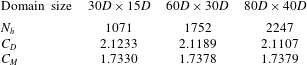
In figure 31,
 $N_{p}$
-convergence is checked at
 $\unicode[STIX]{x1D6FD}=100$
, which is the maximum Stokes number (for smallest
 $\unicode[STIX]{x1D6FF}$
) in this study, on meshes
 $e/D=0.25$
and 0.5, where the blockage effect is strong. Differences between the results are negligible, which suggests that
 $N_{p}=7$
is sufficient to produce converged results for the thinnest shear layer in this study. The 2-D and 3-D Floquet analyses results are validated against Elston et al. (Reference Elston, Blackburn and Sheridan2006) for an isolated cylinder. Figure 32(a) compares the real and imaginary parts of the critical Floquet eigenfunction with respect to 2-D
 $K_{x}$
symmetry breaking and figure 32(b) compares the isosurface of 3-D instability in regime D. Figures 32(c) and 32(d) further quantitatively compare the critical curves for symmetry breaking at
 $3<KC<10$
and the variation of Floquet multiplier as functions of wavenumber
 $k$
for the three-dimensional secondary instability of regime D at
 $(KC,\unicode[STIX]{x1D6FD})=(8,10.85)$
. These results all show good agreement among them.
Appendix B. Stabilization method
The algorithm of the stabilization method employed in the present study for
 $H_{1}$
symmetric flow is demonstrated in figure 33 and is briefly introduced below:
(i) evolve the flow field by solving the Navier–Stokes equations in half of a flow period from
$u(t_{i})$
to
$u(t_{i}+T/2)$
;(ii) obtain the mirrored flow field
$u_{r}(t_{i}+T/2)$
by reflecting the flow field
$u(t_{i}+T/2)$
about
$x=0$
;(iii) estimate the flow field
$u(t_{i}+T)$
by averaging the flow fields at
$u(t_{i})$
and
$u_{r}(t_{i}+T/2)$
, and uses it as the initial condition for solution process in the next flow period
$t_{i}+1=t_{i}+T$
;(iv) repeat the above procedure until a converged base flow is obtained.


It is validated against transition from regime D to E for an isolated cylinder. The DNS results show that the flow remains
 $H_{1}$
symmetric up to 28 by employing successive initialization with interval
 $\unicode[STIX]{x0394}\unicode[STIX]{x1D6FD}=1$
(figure 34
a,b). The intermittently flip of
 $C_{L}$
at
 $\unicode[STIX]{x1D6FD}=28.5$
indicates the flow is in regime E (figure 34
c) with zero IC. Even for such a flow, the
 $H_{1}$
symmetric base flow has been obtained by implementing the stabilization method proposed in this study (figure 34
d). The predicted critical Stokes number
 $\unicode[STIX]{x1D6FD}_{cr_{\infty }}=28.3$
from the base flow agrees well with DNS (28–29) and experimental results (
 ${\sim}28$
).