1 Introduction
Highly three-dimensional geometries associated with supersonic engine intakes and control surfaces can induce complex shock systems which promote shock boundary layer interactions (SBLIs) and potentially undesirable effects. These often swept interactions can significantly influence efficiency, unsteady loading and surface heating (Dolling Reference Dolling2001). It is therefore of paramount importance to understand three-dimensional (3-D) SBLIs so that designs may be improved in future vehicles. Fundamental studies of various shock boundary layer interactions (SBLIs) have often sought to retain a non-dimensional form, whereby the only length scale is the boundary layer which offers a more generalised flow field (Settles & Dolling Reference Settles, Dolling and Hemsch1992). The introduction of sweep retains this form, enabling further analysis of fundamental SBLI physics.
SBLIs featuring swept impinging oblique shocks are poorly understood due to a lack of research on this unique configuration. Until recently, only one study has been reported in literature and is limited to hypersonic flow (Holden Reference Holden1984). A renewed interest in sustained high-speed atmospheric flight has fuelled recent research efforts that show complex flow fields with separated flow and significant unsteadiness (Hainsworth, Dawson-Ruiz & Little Reference Hainsworth, Dawson-Ruiz and Little2014; Dawson-Ruiz, Pederson & Little Reference Dawson-Ruiz, Pederson and Little2015; Gross & Fasel Reference Gross and Fasel2016; Threadgill et al. Reference Threadgill, Stab, Doehrmann and Little2017; Doehrmann et al. Reference Doehrmann, Padmanabhan, Threadgill and Little2018; Gross, Little & Fasel Reference Gross, Little and Fasel2018). While 3-D SBLIs have been subject to investigation by the aerospace research community, a fundamental parametric appreciation of the various intricacies related to swept impinging oblique SBLIs remains unexplored.
Various other types of swept SBLI have been studied in a range of configurations, most notably for interactions induced by straight sharp fins (Settles & Kimmel Reference Settles and Kimmel1986; Lu, Settles & Horstman Reference Lu, Settles and Horstman1990; Lu & Settles Reference Lu and Settles1990; Alvi & Settles Reference Alvi and Settles1992; Lu Reference Lu1993) and swept compression ramps (Bachalo Reference Bachalo1975; Settles, Perkins & Bogdonoff Reference Settles, Perkins and Bogdonoff1980; Settles & Bogdonoff Reference Settles and Bogdonoff1982; Settles & Teng Reference Settles and Teng1984; Settles, Horstman & McKenzie Reference Settles, Horstman and McKenzie1986; Erengil & Dolling Reference Erengil and Dolling1993). Such configurations generate a shock system that interacts with the incoming boundary layer along a swept line. The addition of leading edge sweep to a sharp fin induces a swept oblique shock that is directly relatable to the present study. However, this configuration has also attracted little attention in the open literature despite its widespread prevalence in practice (Settles & Lu Reference Settles and Lu1985).
Two dominant scaling similarities have been reported when characterising the structure of swept SBLIs. The glancing interactions associated with sharp fins and highly swept compression ramps retain conical similarities which demonstrate a growth of length scales as the interaction develops in the direction of sweep (Settles & Teng Reference Settles and Teng1984; Settles & Lu Reference Settles and Lu1985; Lu Reference Lu1993). The situation for lesser swept interactions induced by compression ramps is more ambiguous. Early studies reported a cylindrical similarity (Settles & Teng Reference Settles and Teng1984); however, it is not yet clear if this observation is influenced by the limited domain size associated with most supersonic wind tunnel tests (Vanstone & Clemens Reference Vanstone and Clemens2018). Regardless, two isolated regimes of interaction development have been observed (cylindrical/conical).
The effect of sweep on SBLI unsteadiness remains under investigation (Erengil & Dolling Reference Erengil and Dolling1993; Arora, Ali & Alvi Reference Arora, Ali and Alvi2016; Adler & Gaitonde Reference Adler and Gaitonde2017; Vanstone et al. Reference Vanstone, Hashemi, Lingren, Akella, Clemens, Donbar and Gogineni2017a; Doehrmann et al. Reference Doehrmann, Padmanabhan, Threadgill and Little2018). In two-dimensional SBLIs, a low-frequency motion of the separation shock foot has been observed across various configurations with a time scale approximately two orders of magnitude above that of the incoming boundary layer (Clemens & Narayanaswamy Reference Clemens and Narayanaswamy2014). The characteristic frequency of this peak generally moves toward higher frequencies as the angle of sweep is increased. Numerous possible mechanisms have been proposed to explain the shift in frequency: (i) reduction in separation shock motion with sweep while separation-normal shock velocities remain constant (Erengil & Dolling Reference Erengil and Dolling1993), (ii) spanwise travelling separation structures moving with cross-flow velocity (Vanstone et al. Reference Vanstone, Bosco, Saleh, Akella, Clemens and Gogineni2019), (iii) accelerating spanwise shock ripples with constant frequency imposed at the interaction root (Padmanabhan et al. Reference Padmanabhan, Castro Maldonado, Threadgill and Little2019) and (iv) suggestions that no low frequency is present when interaction sweep promotes open separation (Adler & Gaitonde Reference Adler and Gaitonde2017). However, none of these mechanisms have yet fully established a consensus on their role.
Before details of the SBLIs are assessed with regards to sweep, it is important to note that there appears to be a broad oversimplification in the literature on the influence of sweep on the incident shock itself. A common misconception is that sweep simply adds an additional component of velocity running parallel to the shock which can be disregarded as it will not change across the shock. While it is true that this velocity component is present, it does not fully evaluate changes to the shock due to sweep. A feature often overlooked is that as sweep increases, the deflection angle normal to the sweep also increases, affecting shock strength. It is well known that two-dimensional turbulent SBLIs scale with the inviscid pressure rise across an interaction (Morgan et al. Reference Morgan, Duraisamy, Nguyen, Kawai and Lele2013; Souverein, Bakker & Dupont Reference Souverein, Bakker and Dupont2013). It is reasonable to assume that 3-D SBLIs will follow suit, particularly for moderate sweep. Subtle changes in the inviscid pressure rise due to sweep are expected to be important, especially in laminar and transitional SBLIs. Thus, accurate understanding/prediction of the inviscid behaviour is essential for the study 3-D SBLIs.
For inviscid swept compression ramp flows, the shock is anchored to the ramp corner (when inducing an attached oblique shock). Variations of the shock (in terms of strength and angle) caused by moderate changes in sweep for a given  $x$–
 $y$ plane ramp deflection are often overlooked since the influence can be small. While such variance has been observed in inviscid flows (Domel Reference Domel2016; Threadgill et al. Reference Threadgill, Stab, Doehrmann and Little2017), their influence in viscous interactions has not been factored into characterisation studies.
Infinite-span swept oblique inviscid shock structures have been modelled in an important contribution by Domel (Reference Domel2016), who extend the standard two-dimensional  $\unicode[STIX]{x1D703}{-}\unicode[STIX]{x1D6FD}{-}M$ relations to a three-dimensional
 $\unicode[STIX]{x1D703}{-}\unicode[STIX]{x1D6FD}{-}M{-}\unicode[STIX]{x1D713}$ form to include the influence of sweep on oblique shocks. The model is formulated in terms of a cubic expression that can be solved to determine shock characteristics. However, the specific formulation is primarily applicable to single-shock structures (such as those from swept sharp-fin or compression ramps). Without significant manipulation, it is therefore of limited application to multiple-shock configurations with exception of validating the initial shock (Threadgill et al. Reference Threadgill, Stab, Doehrmann and Little2017). In addition, the implications of limited span oblique shocks that can be critical in moderate aspect ratio flows associated with engine inlets and highly swept delta wings are not modelled.
For interactions limited in the spanwise direction by a zero spanwise mass flux criterion (either through an experimental symmetry plane (Settles & Lu Reference Settles and Lu1985), simulation slip plane (Adler & Gaitonde Reference Adler and Gaitonde2017; Gross et al. Reference Gross, Little and Fasel2018) or an endplate/fence (Threadgill et al. Reference Threadgill, Stab, Doehrmann and Little2017; Vanstone et al. Reference Vanstone, Saleem, Seckin and Clemens2017b)) the shock angle also changes at this location (Settles & Lu Reference Settles and Lu1985). This effect is small for inviscid swept compression ramp flows since the shock foot is anchored to the ramp corner. However, it cannot be overlooked in swept impinging oblique SBLIs since changes in the shock angle alters the wall impingement location, meaning the interaction is no longer anchored at a region on the wall that runs parallel to the imposed sweep. Such an influence is not encountered in unswept sharp-fin flows since the inviscid flow remains two-dimensional. However, it has a significant effect on swept sharp fins since the inviscid shock location at the wall does not agree with simple 2-D shock theory (Settles & Lu Reference Settles and Lu1985).
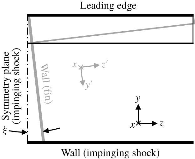
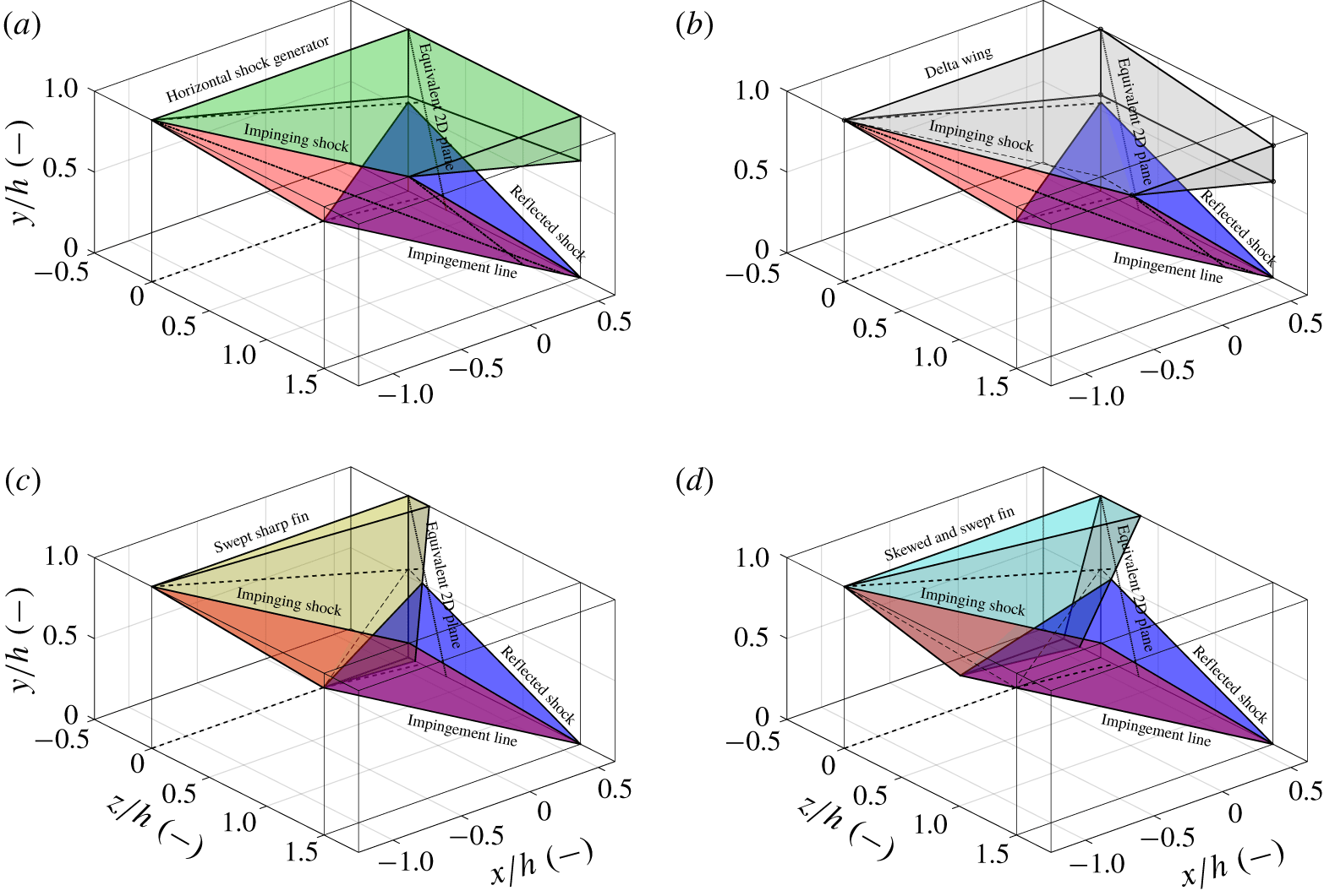
Since the incident swept oblique shock is inclined from normal in both the  $x$–
 $y$ and
 $x$–
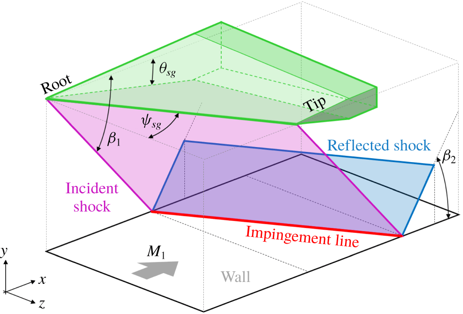
 $z$ planes (see figure 1), one would expect an element of spanwise cross-flow in addition to the downward flow deflection induced by the shock generator (Domel Reference Domel2016). After encountering the reflected shock this effect would be amplified, creating a component of spanwise flow that would be experienced downstream of the interaction. Modification of this cross-flow through the use of a fence (Vanstone & Clemens Reference Vanstone and Clemens2018), symmetry plane (Settles & Lu Reference Settles and Lu1985) or root plane leakage effects (Threadgill et al. Reference Threadgill, Stab, Doehrmann and Little2017) would influence this injection of mass into the swept SBLI, causing the shocks to change in strength to account for the downstream divergence (analogous to two-dimensional versus axisymmetric compression ramps). This will result in a spanwise pressure gradient within the interaction near the root plane, and a curved shock–wall impingement line in the case of a swept oblique impinging SBLI. Such influences will distort the flow beyond 2-D features present in a quasi-infinite-span configuration.
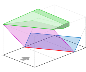
Inviscid shock schematic diagram. The incident shock is shown in magenta, the reflected shock is shown in blue. The incident shock–wall impingement line is shown in red.

The mechanisms driving the appearance of conical similarity for swept SBLIs remain unclear, but have been associated with inviscid flow detachment (Settles & Teng Reference Settles and Teng1984). In swept compression ramp flows, the addition of sweep decreases the  $x$–
 $y$ plane flow deflection angle required to induce inviscid flow detachment. The boundary between cylindrical/conical similarities occurs at similar conditions, albeit at approximately
 $10^{\circ }$ sweep below that required to induce detachment (Settles & Teng Reference Settles and Teng1984). Understanding these consequences when applied to the more complex interaction studied herein requires a robust method for estimating the onset of flow detachment.
Finally, understanding the influence of sweep on wave drag is an important feature to consider in vehicle design. Two-dimensional shock bump studies have shown a decrease in shock-induced drag when located on a transonic wing during cruise (Bruce & Colliss Reference Bruce and Colliss2015). Similarly, the addition of sweep to transonic airfoil flows is well established for decreasing shock strength by reducing the normal component of flow through the terminating normal shock. However, in some supersonic conditions sweep has been theoretically predicted to increase total pressure loses (Threadgill et al. Reference Threadgill, Stab, Doehrmann and Little2017). In summary, despite significant practical relevance, a detailed understanding regarding the effect of sweep on the inviscid features of oblique shock reflections has not been established and is investigated herein.
Two-dimensional oblique shock theory is well established (Anderson Reference Anderson2004) and will not be presented here for brevity. Application of such theory has been conducted for single-shock swept compression ramps (Domel Reference Domel2016) and demonstrates the ability to predict the inviscid shock structure for a given ramp geometry. While not directly predicting the viscous interaction structure, similar inviscid models have been used with some success to provide a baseline for the interaction (Délery Reference Délery1985). It should be noted that a wealth of supporting experimental data for inviscid shock structures can be extracted from investigations of free-stream delta-wing flows (Messiter Reference Messiter1963; Squire Reference Squire1968; Voskresenskii Reference Voskresenskii1968; Roe Reference Roe1970; Klunker, South & Davis Reference Klunker, South and Davis1971; Settles & Lu Reference Settles and Lu1985). This provides ample opportunity for inviscid model validation and comparison to the viscous reality.
The objective of this work is to create a 3-D inviscid model of a swept shock reflection to contextualise SBLI conditions across a variety of swept configurations, and to place the associated findings as they relate to viscous behaviour in context. Section 2 details the model with supporting validation studies, § 3 demonstrates application of the model for a given flow environment, § 4 reviews pertinent observations through interrogation of the model and conclusions are presented in § 5.
2 Model description
The model geometry employed herein is defined in figure 1. The  $x$–
 $y$–
 $z$ reference frame is set by: (
 $x$) the incoming flow vector, (
 $y$), the wall-normal vector and (
 $z$), the resultant spanwise vector. Three-dimensional velocity components
 $u$–
 $v$–
 $w$ are defined relative to the
 $x$–
 $y$–
 $z$ reference frame, respectively. A swept shock generator is located above the wall and is defined according to the
 $x{-}y{-}z$-reference frame to retain a fundamental approach. The leading edge is located in the
 $x$–
 $z$ plane and runs parallel to the wall. Sweep
 $\unicode[STIX]{x1D713}$ is defined in the
 $x$–
 $z$ plane as the rotation of the leading edge vector around the
 $y$ axis, relative to the
 $z$ axis. The angle of the shock generator surface relative to the incoming flow is defined in the
 $x$–
 $y$ plane relative to the
 $x$ axis. The downward flow deflection beneath the shock generator produces a swept oblique shock which impinges upon the wall. By imposing a slip-plane condition on the wall the incident shock is reflected and forms a second swept oblique shock. The model is defined in an infinite-span configuration to present solutions in a spanwise homogeneous canonical form, resulting a quasi-2-D flow field (the influences of spanwise-limiting effects are discussed further in § 4.5). Where dimensional values have been quoted, the gas medium is assumed to be an inviscid perfect gas, with
 $\unicode[STIX]{x1D6FE}=1.4$ and
 $R=287.1~\text{J}~\text{kg}^{-1}~\text{K}^{-1}$ to reflect dry air. Flow across shocks is considered to be adiabatic, as are conditions at the wall.
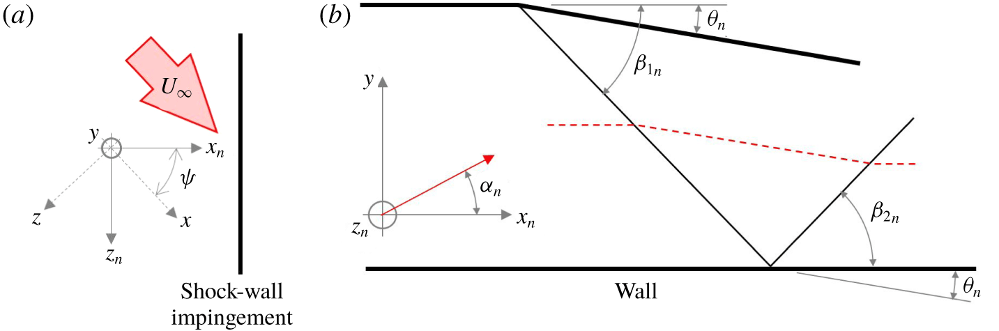
The application of continuity across an oblique shock mandates that the components of velocity running parallel to the shock are conserved. For convenience, the reference frame is transformed via rotation about the  $y$ axis using transformation matrix
 $\unicode[STIX]{x1D73F}$ to be aligned with the incident shock–wall impingement line, such that the transformed
 $z_{n}$ axis runs parallel to this line (Gross & Fasel Reference Gross and Fasel2016) (see figure 2 and equation (2.1)).
 $$\begin{eqnarray}\left[\begin{array}{@{}c@{}}u_{n}\\ v\\ w_{n}\end{array}\right]=\unicode[STIX]{x1D73F}\left[\begin{array}{@{}c@{}}u\\ v\\ w\end{array}\right]=\left[\begin{array}{@{}l@{}}u\cos \unicode[STIX]{x1D713}-w\sin \unicode[STIX]{x1D713}\\ v\\ u\sin \unicode[STIX]{x1D713}+w\cos \unicode[STIX]{x1D713}\end{array}\right],\end{eqnarray}$$
where
 $$\begin{eqnarray}\unicode[STIX]{x1D73F}=\left[\begin{array}{@{}ccc@{}}\cos \unicode[STIX]{x1D713} & 0 & -\text{sin}\,\unicode[STIX]{x1D713}\\ 0 & 1 & 0\\ \sin \unicode[STIX]{x1D713} & 0 & \cos \unicode[STIX]{x1D713}\end{array}\right].\end{eqnarray}$$
Inviscid shock schematic diagram, rotated around the  $z^{\prime }$-axis such that the side view in the
 $x_{n}$–
 $y$ plane is aligned with the shock. (a) Top view (
 $x$–
 $z$ or
 $x_{n}$–
 $z_{n}$ plane). (b) Side view (
 $x_{n}$–
 $y$ plane).

Since the  $z_{n}$-axis runs parallel to the wall impingement line, it also runs parallel to both shocks. Therefore, the
 $w_{n}$ velocity component is considered constant across the entire shock reflection. Equation (2.2) is used to determine velocity magnitude (
 $U$) as a function of total temperature
 $T_{0}$, with the sweep-aligned velocity component established using (2.3). By disregarding this velocity component, the equivalent incoming Mach number for a two-dimensional shock reflection in the
 $x_{n}$–
 $y_{n}$ plane is identified using equation (2.4).
 $$\begin{eqnarray}\displaystyle & \displaystyle U^{2}=\frac{2\unicode[STIX]{x1D6FE}RT_{0}M^{2}}{2+\left(\unicode[STIX]{x1D6FE}-1\right)M^{2}}, & \displaystyle\end{eqnarray}$$
 $$\begin{eqnarray}\displaystyle & \displaystyle w_{n}=U_{\infty }\sin \unicode[STIX]{x1D713}, & \displaystyle\end{eqnarray}$$
 $$\begin{eqnarray}\displaystyle & \displaystyle {M_{\infty }}_{n}=M_{\infty }\cos \unicode[STIX]{x1D713}. & \displaystyle\end{eqnarray}$$
The flow deflection angle in the  $x_{n}$–
 $y$ plane will be steeper than that measured on the shock generator in the
 $x$–
 $y$ plane due to the addition of sweep. This angle is calculated using (2.5). Determination of the remaining flow structure in the
 $x_{n}$–
 $y$ plane follows a standard two-dimensional approach with well-established relations. Shock angle
 $\unicode[STIX]{x1D6FD}_{n}$ and incoming flow angle
 $\unicode[STIX]{x1D6FC}_{n}$ are defined relative to the
 $x_{n}$–
 $z_{n}$ plane (all angles are defined with same rotation direction around the
 $z_{n}$ axis for a given shock, such that
 $\unicode[STIX]{x1D6FD}_{n}$ and
 $\unicode[STIX]{x1D703}_{n}$ are positive). Equation (2.6) is used to find the shock angle in the
 $x_{n}$–
 $y$ plane, with the downstream
 $x_{n}$–
 $y$ plane Mach number given by (2.7) (subscripts
 $a$ and
 $b$ indicate conditions upstream or downstream of the shock being analysed, respectively).
 $$\begin{eqnarray}\displaystyle & \displaystyle \tan \unicode[STIX]{x1D703}_{n}=\frac{\tan \unicode[STIX]{x1D703}_{sg}}{\cos \unicode[STIX]{x1D713}}, & \displaystyle\end{eqnarray}$$
 $$\begin{eqnarray}\displaystyle & \displaystyle \tan \unicode[STIX]{x1D703}_{n}=\frac{2}{\tan \left(\unicode[STIX]{x1D6FD}_{n}-\unicode[STIX]{x1D6FC}_{n}\right)}\left\{\frac{{M_{a}}_{n}^{2}\sin ^{2}\left(\unicode[STIX]{x1D6FD}_{n}-\unicode[STIX]{x1D6FC}\right)-1}{{M_{a}}_{n}^{2}\left[\unicode[STIX]{x1D6FE}+\cos \left(2\unicode[STIX]{x1D6FD}_{n}-2\unicode[STIX]{x1D6FC}_{n}\right)\right]+2}\right\}, & \displaystyle\end{eqnarray}$$
 $$\begin{eqnarray}\displaystyle & \displaystyle {M_{b}}_{n}^{2}\sin ^{2}\left(\unicode[STIX]{x1D6FD}_{n}-\unicode[STIX]{x1D6FC}_{n}-\unicode[STIX]{x1D703}_{n}\right)=\frac{2+\left(\unicode[STIX]{x1D6FE}-1\right){M_{a}}_{n}^{2}\sin ^{2}\left(\unicode[STIX]{x1D6FD}_{n}-\unicode[STIX]{x1D6FC}_{n}\right)}{2\unicode[STIX]{x1D6FE}{M_{a}}_{n}^{2}\sin ^{2}\left(\unicode[STIX]{x1D6FD}_{n}-\unicode[STIX]{x1D6FC}_{n}\right)-2\left(\unicode[STIX]{x1D6FE}-1\right)}. & \displaystyle\end{eqnarray}$$
The inclination of the shock and the downstream flow vector are first found in the  $x_{n}$–
 $y$ plane, before applying the inverse transformation matrix from (2.1). The shock inclination is defined using a unit vector normal to the shock plane given by (2.8), where
 $\unicode[STIX]{x1D6FC}_{n}$ is the angle of the incoming flow relative to the
 $x_{n}$–
 $z_{n}$ plane.
 $$\begin{eqnarray}\boldsymbol{N}_{n}=\left[\begin{array}{@{}c@{}}\sin \unicode[STIX]{x1D6FD}_{n}\\ \cos \unicode[STIX]{x1D6FD}_{n}\\ 0\end{array}\right].\end{eqnarray}$$
The downstream flow is similarly defined using a unit vector, which requires recombining velocity components downstream of the shock. While the  $w_{n}$ component is already known from (2.3), definition of
 $u_{n}$ and
 $v$ components necessitates finding the downstream Mach number
 $M_{2}$ using (2.9), which is then converted back to flow speed
 $U$ using (2.2). The velocity magnitude in the
 $x_{n}$–
 $y$ plane is then given by (2.10), with the flow unit vector given by (2.11).
 $$\begin{eqnarray}\displaystyle & \displaystyle M^{2}=\frac{M_{n}^{2}+{\displaystyle \frac{w_{n}^{2}}{\unicode[STIX]{x1D6FE}RT_{0}}}}{1-(\unicode[STIX]{x1D6FE}-1){\displaystyle \frac{w_{n}^{2}}{2\unicode[STIX]{x1D6FE}RT_{0}}}}=\frac{M_{n}^{2}\left[2+M_{\infty }^{2}\left(\unicode[STIX]{x1D6FE}-1\right)\right]+2M_{\infty }^{2}\sin ^{2}\unicode[STIX]{x1D713}}{2+M_{\infty }^{2}(\unicode[STIX]{x1D6FE}-1)\left(1-\sin ^{2}\unicode[STIX]{x1D713}\right)}, & \displaystyle\end{eqnarray}$$
 $$\begin{eqnarray}\displaystyle & \displaystyle U_{n}^{2}=U^{2}-w_{n}^{2}, & \displaystyle\end{eqnarray}$$
 $$\begin{eqnarray}\displaystyle & \displaystyle \boldsymbol{a}_{n}=\left[\begin{array}{@{}c@{}}u_{n}\\ v\\ w_{n}\end{array}\right]=\frac{1}{U}\left[\begin{array}{@{}c@{}}U_{n}\cos \unicode[STIX]{x1D6FC}_{n}\\ U_{n}\sin \unicode[STIX]{x1D6FC}_{n}\\ U_{\infty }\sin \unicode[STIX]{x1D713}\end{array}\right]=\frac{M_{\infty }}{M}\sqrt{\frac{T_{\infty }}{T}}\left[\begin{array}{@{}c@{}}\unicode[STIX]{x1D6EC}\cos \unicode[STIX]{x1D6FC}_{n}\\ -\unicode[STIX]{x1D6EC}\sin \unicode[STIX]{x1D6FC}_{n}\\ \sin \unicode[STIX]{x1D713}\end{array}\right], & \displaystyle\end{eqnarray}$$
where
 $$\begin{eqnarray}\unicode[STIX]{x1D6EC}=\sqrt{\frac{M^{2}T}{M_{\infty }^{2}T_{\infty }}-\sin ^{2}\unicode[STIX]{x1D713}}.\end{eqnarray}$$
Unit vectors describing shock inclination and flow direction in the  $x_{n}$–
 $y$ plane are then transformed, using the
 $\unicode[STIX]{x1D73F}^{\prime }$ transformation matrix in (2.1), to return components in the
 $x-y-z$ reference frame (see (2.12) and (2.13)). The ratio
 $T_{\infty }/T$ is calculated using adiabatic relations (see (2.14)).
 $$\begin{eqnarray}\displaystyle & \displaystyle \boldsymbol{N}=\unicode[STIX]{x1D73F}^{\prime }\boldsymbol{N}_{n}=\sin \unicode[STIX]{x1D6FD}_{n}\left[\begin{array}{@{}c@{}}\cos \unicode[STIX]{x1D713}\\ 1/\text{tan}\unicode[STIX]{x1D6FD}_{n}\\ -\text{sin}\,\unicode[STIX]{x1D713}\end{array}\right], & \displaystyle\end{eqnarray}$$
 $$\begin{eqnarray}\displaystyle & \displaystyle \boldsymbol{a}=\unicode[STIX]{x1D73F}^{\prime }\boldsymbol{a}_{n}=\left[\begin{array}{@{}c@{}}\sin ^{2}\unicode[STIX]{x1D713}+\unicode[STIX]{x1D6EC}\cos \unicode[STIX]{x1D6FC}_{n}\cos \unicode[STIX]{x1D713}\\ -\unicode[STIX]{x1D6EC}\sin \unicode[STIX]{x1D6FC}_{n}\\ \sin \unicode[STIX]{x1D713}\left(\cos \unicode[STIX]{x1D713}-\unicode[STIX]{x1D6EC}\cos \unicode[STIX]{x1D6FC}_{n}\right)\end{array}\right]\frac{M_{\infty }}{M}\sqrt{\frac{T_{\infty }}{T}}, & \displaystyle\end{eqnarray}$$
 $$\begin{eqnarray}\displaystyle & \displaystyle \frac{T_{\infty }}{T}=\frac{2+(\unicode[STIX]{x1D6FE}-1)M^{2}}{2+(\unicode[STIX]{x1D6FE}-1)M_{\infty }^{2}}. & \displaystyle\end{eqnarray}$$
Pertinent angles of the flow structure are determined from these vectors. The  $x$–
 $y$ plane shock angle is given by (2.15), the
 $x$–
 $y$ plane flow deflection angle is given by (2.16), the
 $x$–
 $z$ plane spanwise deflection angle is given by (2.17) and the
 $y$–
 $z$ plane flow rotation angle, which defines the effective two-dimensional oblique shock plane (Domel Reference Domel2016), is given by (2.18).
 $$\begin{eqnarray}\displaystyle & \displaystyle \tan \unicode[STIX]{x1D6FD}=N_{x}/N_{y}=\cos \unicode[STIX]{x1D713}\cdot \tan \unicode[STIX]{x1D6FD}_{n}, & \displaystyle\end{eqnarray}$$
 $$\begin{eqnarray}\displaystyle & \displaystyle \tan \unicode[STIX]{x1D703}=a_{y}/a_{x}=\frac{-\unicode[STIX]{x1D6EC}\sin \unicode[STIX]{x1D6FC}_{n}}{\sin ^{2}\unicode[STIX]{x1D713}+\unicode[STIX]{x1D6EC}\cos \unicode[STIX]{x1D6FC}_{n}\cos \unicode[STIX]{x1D713}}, & \displaystyle\end{eqnarray}$$
 $$\begin{eqnarray}\displaystyle & \displaystyle \tan \unicode[STIX]{x1D702}=a_{z}/a_{x}=\frac{\cos \unicode[STIX]{x1D713}-\unicode[STIX]{x1D6EC}\cos \unicode[STIX]{x1D6FC}_{n}}{\sin \unicode[STIX]{x1D713}+\unicode[STIX]{x1D6EC}{\displaystyle \frac{\cos \unicode[STIX]{x1D6FC}_{n}}{\tan \unicode[STIX]{x1D713}}}}, & \displaystyle\end{eqnarray}$$
 $$\begin{eqnarray}\displaystyle & \displaystyle \tan \unicode[STIX]{x1D719}=a_{z}/a_{y}=\sin \unicode[STIX]{x1D713}\left(\frac{1}{\tan \unicode[STIX]{x1D6FC}_{n}}-\frac{\cos \unicode[STIX]{x1D713}}{\unicode[STIX]{x1D6EC}\sin \unicode[STIX]{x1D6FC}_{n}}\right). & \displaystyle\end{eqnarray}$$
Finally, angles of flow deflection and shocks defined on the effective 2-D plane are given by (2.19) and (2.20), respectively.
 $$\begin{eqnarray}\displaystyle & \displaystyle \tan \unicode[STIX]{x1D703}_{e}=\frac{\tan \unicode[STIX]{x1D703}_{sg}\cos \unicode[STIX]{x1D709}}{\cos \left(\unicode[STIX]{x1D719}-\unicode[STIX]{x1D709}\right)}, & \displaystyle\end{eqnarray}$$
 $$\begin{eqnarray}\displaystyle & \displaystyle \tan \unicode[STIX]{x1D6FD}_{e}=\tan \unicode[STIX]{x1D6FD}\cos \unicode[STIX]{x1D719}, & \displaystyle\end{eqnarray}$$
where
 $$\begin{eqnarray}\tan \unicode[STIX]{x1D709}=\tan \unicode[STIX]{x1D703}_{sg}\tan \unicode[STIX]{x1D713}.\end{eqnarray}$$
3 Results
3.1 Summary of results
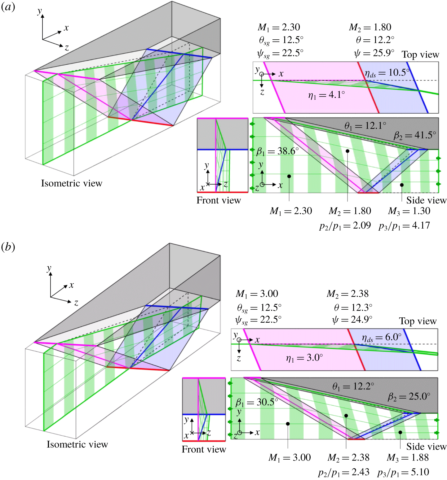
Implementation of the inviscid model above is shown in figure 3 for two example flows with upstream Mach numbers of 2.3 and 3.0, each encountering a moderately swept shock generator ( $\unicode[STIX]{x1D713}=22.5^{\circ }$ and
 $\unicode[STIX]{x1D703}=12.5^{\circ }$) mounted parallel to a slip-wall floor below. Incoming flow encounters the incident shock and is deflected downwards and towards the angle of sweep. Since the inviscid flow downstream of the shock must remain parallel to the shock generator face, the resultant deflection may be considered as a combination of two components: (i)
 $x$–
 $y$ plane deflection that is below that of the shock generator (as flow passes the face towards the tip), and (ii) the additional
 $x$–
 $z$ plane deflection induced by the oblique sweep angle.
Both flows clearly demonstrate the key features of inviscid shock reflections, namely that flow downstream of the reflection is: (i) parallel to the wall, (ii) deflected towards the sweep angle, (iii) negatively skewed in the  $x$–
 $y$ plane and (iv) positively skewed in the
 $x$–
 $z$ plane. In addition, shock inclination changes with sweep leading to variable strength shocks affecting downstream pressure rise.
Inviscid flow fields with  $\unicode[STIX]{x1D713}=22.5^{\circ }$ and
 $\unicode[STIX]{x1D703}_{sg}=12.5^{\circ }$. The shock generator is shown in grey. The incident shock is shown in magenta, the reflected shock is shown in blue. The incident shock–wall impingement line is shown in red. Streamlines are shown by thin green lines, and timelines are shown by broad green regions. The dashed black line indicates a cross-section of the shock system in the
 $x$–
 $y$ plane. Geometries are shown to scale. (a) Mach 2.3. (b) Mach 3.0.

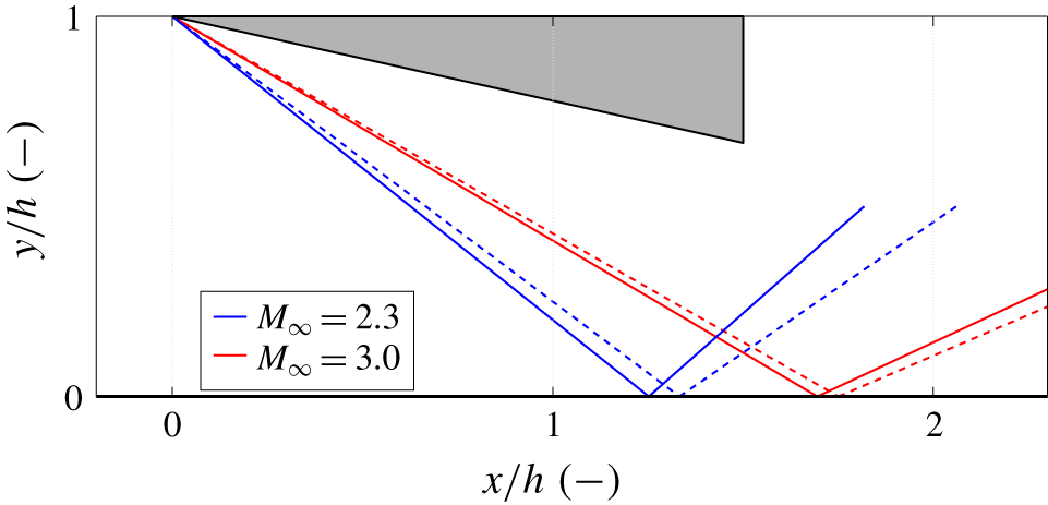
Figure 4 shows a corresponding shock structure plot extracted in an  $x$–
 $y$ plane, equivalent to commonly reported particle image velocimetry (PIV) domains. The effect of a sweep is clearly evident, increasing steepness of shocks and moving the wall impingement location further upstream.
The  $x$–
 $y$ plane shock structure normalised by shock generator height
 $h$, demonstrating the effect of sweep for various incoming Mach numbers. Shock generator with deflection
 $\unicode[STIX]{x1D703}_{sg}=12.5^{\circ }$ is shown in grey. Swept shocks at
 $\unicode[STIX]{x1D713}=22.5^{\circ }$ are shown with solid lines, unswept shocks are shown with dashed lines.

3.2 Model limitations
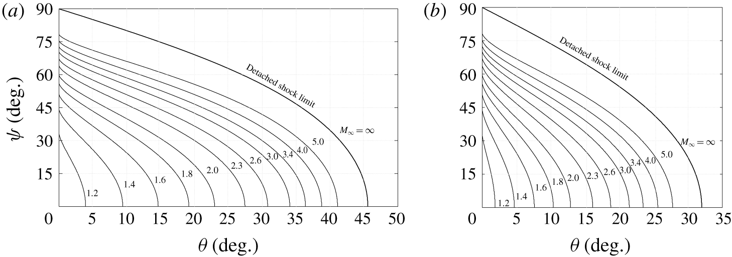
The model above relies on analytical inviscid flow relations. It is therefore not applicable when inviscid shock detachment occurs as flow is deflected beyond the maximum turning angle for a given local upstream Mach number. In such situations, the shock will translate upstream and curve towards the wall to form a local subsonic region (in a plane normal to the sweep angle) that enables flow to achieve the required deflection. The structure of this region is not analytically solvable (Settles & Lu Reference Settles and Lu1985) and is therefore beyond the scope of this model. Regardless, the onset of this regime is clearly defined such that at conditions below the detachment onset boundary the present model is valid. Prediction of the onset of shock detachment is particularly relevant in swept SBLI studies as this has been proposed to act as a mechanism that changes the interaction from cylindrical (i.e. parallel lines of separation and reattachment) to conical (i.e. divergent separation and reattachment lines) (Settles & Teng Reference Settles and Teng1984).
Onset of shock detachment in the oblique shock reflection configuration. Geometries that fall below or to the left of the contours represent flows that would induce an attached shock. (a) Incident shock. (b) Reflected shock.

As with unswept oblique shocks, there are two potential inviscid shock solutions for a given sweep–Mach number combination: a steep strong shock with subsonic downstream flow (when observed in the sweep-aligned  $x_{n}$–
 $y$ plane), or a shallower weak shock which typically exhibits local supersonic downstream flow (except at conditions close to the maximum turning angle where it too may return subsonic flow). While it is weak shock solutions that would usually form in nature, strong oblique shocks may be induced in situations of high imposed back pressure (Anderson Reference Anderson2004). Full implementation of the above model requires that flow must be supersonic downstream of the incident shock (when viewed in the
 $x_{n}$–
 $y$ plane), thus limiting the incident shock solution to the supersonic weak case only. The reflected shock may exhibit either solution through selection of the appropriate
 $\unicode[STIX]{x1D6FD}_{n}$. If the required deflection to redirect flow parallel to the floor is greater than the maximum turning angle then the reflected shock will detach to form a Mach reflection (Ben-Dor Reference Ben-Dor2007) (as opposed to the regular reflection studied herein) and the model becomes invalid.
Figure 5 demonstrates the onset of the maximum turning angle limitations with respect to shock generator  $x$–
 $y$ deflection and sweep, which is of importance when considering the proposed onset of conical/cylindrical SBLI development (Settles & Teng Reference Settles and Teng1984). Increasing the upstream Mach number expands the available envelope for both sweep and shock generator deflection angles. Sweep at low angles of shock generator deflection is limited by the local upstream Mach wave angle such that
 $\unicode[STIX]{x1D713}\leqslant 90^{\circ }-\unicode[STIX]{x1D707}$. Above this limit at
 $\unicode[STIX]{x1D703}=0^{\circ }$, the local upstream Mach number component normal to the sweep is subsonic and does not induce a shock. However, below this upper limit in sweep excessive flow deflection beyond the maximum turning angle will result in shock detachment. At the zero-sweep limit this aligns with unswept 2-D shock detachment. The behaviour across the reflected shock is similar in nature to the incident shock, albeit shifted towards lower shock generator deflection angles. This is due to the reduction in Mach number across the incident shock, an effect which diminishes at low deflection angles, and is evident by maintaining the same zero-deflection sweep limit as for the incident shock case.
4 Discussion
4.1 Collapse of sweep influence
Initial observation of the results would suggest that flow configuration is subject to three input terms: (i) upstream Mach number  $M_{\infty }$, (ii)
 $x$–
 $z$ plane sweep
 $\unicode[STIX]{x1D713}$ and (iii)
 $x$–
 $y$ plane deflection angle
 $\unicode[STIX]{x1D703}_{sg}$. This results in a reasonably complex model imposing difficulties in extracting certain behaviours, as demonstrated by shock detachment predictions given in figure 5. However, certain observations can be made in construction of the model to simplify results.
Determination of the shock strength and associated parameters ( ${M_{2}}_{n}$,
 $p_{2}/p_{1}$,
 $T_{2}/T_{1}$, etc.) are all either defined in the swept
 $x_{n}$–
 $y$ plane or defined as a scalar. Therefore, the three-variable problem stated above can be rephrased in this coordinate system to constrain the influence of sweep only in its effect on the Mach number and deflection angle. The upstream Mach number and shock generator deflection angle should therefore be expressed as the respective component experienced in the plane normal to the sweep (
 $x_{n}$–
 $y$ plane) as given by (2.4) and (2.5), respectively. This manipulation results in the collapse of the three-parameter model into two parameters only, simplifying the parametric approach required.
This approach has been followed in unswept sharp-fin studies which have typically resolved Mach number normal to the swept shock as the relevant scaling term (Alvi & Settles Reference Alvi and Settles1992). Since the shock induced by an unswept sharp fin is not inclined in the  $x$–
 $y$ plane and occurs on a flat plate, it follows that the inviscid flow deflection normal to the sweep is zero and the shock acts as a normal shock with a cross-flow component.
Addition of sweep to the sharp-fin leading edge (or shock generator leading edge) therefore necessitates inclusion of this effect when considering flow parameters across the inviscid shock. The effectiveness of this approach is demonstrated below through a revised prediction of shock detachment, as has been discussed prior in the three-parameter form.
4.2 Detachment phenomena
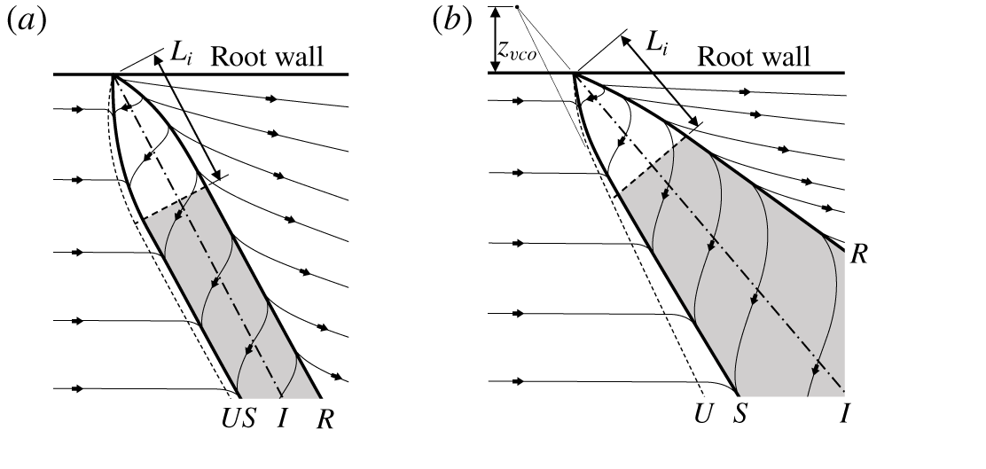
Shock detachment is particularly relevant in swept SBLI research as it has been postulated as a mechanism that brings about a substantial change in interaction behaviour (Settles & Teng Reference Settles and Teng1984). Moderately swept SBLIs with low deflection angles have been observed to develop in the spanwise direction towards a quasi-infinite interaction with length scale  $L_{int}$, presenting cylindrical geometric similarities when scaled (Settles & Teng Reference Settles and Teng1984) (figure 6a). Conversely, highly swept SBLIs with more significant deflection angles demonstrate a continual linear geometric growth of the interaction structure in the spanwise direction described by conical similarities (Settles & Teng Reference Settles and Teng1984; Settles & Kimmel Reference Settles and Kimmel1986) (figure 6b). The mechanism responsible for this change in behaviour is not well understood. However, it has been associated with the following concepts: (i) a fundamental change in 3-D separated flow mass entrainment/ventilation (Settles & Teng Reference Settles and Teng1984), (ii) the onset of shock detachment (Settles & Teng Reference Settles and Teng1984), (iii) sustained influence of the inception region in finite-span domains (Vanstone & Clemens Reference Vanstone and Clemens2018) or (iv) effect of non-planar shock distortion at the root (Settles & Lu Reference Settles and Lu1985; Settles & Kimmel Reference Settles and Kimmel1986).
Schematic diagram of simplified SBLI spanwise development behaviours (adapted from Settles & Teng Reference Settles and Teng1984). Wall topology shows:  $U$ – limit of upstream influence,
 $S$ – separation line,
 $I$ – inviscid shock location,
 $R$ – reattachment line,
 $L_{i}$ – SBLI inception length and
 $z_{VCO}$ – spanwise location of virtual conical origin. Shaded region indicates quasi-infinite development of separated flow. (a) Cylindrical SBLI development. (b) Conical SBLI development.

Determination of the detachment onset boundary has been presented in figure 5 in terms of typical parameters used in experiments and simulations ( $M_{\infty }$,
 $\unicode[STIX]{x1D703}_{sg}$ and
 $\unicode[STIX]{x1D713}$). By instead considering the incoming Mach number and flow deflection components in the
 $x_{n}$–
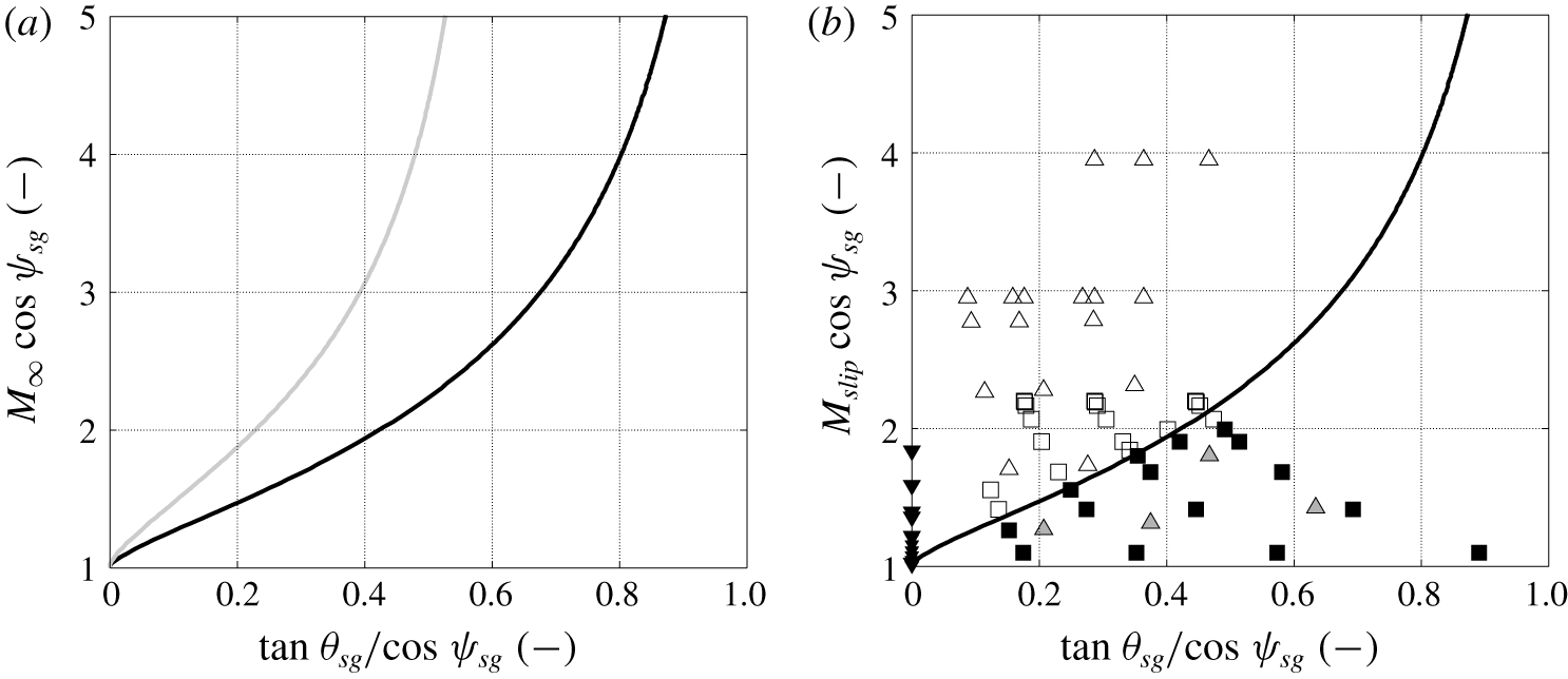
 $y$ plane, this can be plotted as shown in figure 7. The resultant curves now collapse to form unique detachment onset boundaries when solved in a two-parameter domain.
Inviscid model results for both one-shock solutions (i.e. compression ramp or sharp fin) and two-shock solutions (i.e. shock reflection) are shown in figure 7(a). As observed prior, the qualitative nature of the two boundaries appear similar, albeit shifted to higher incoming Mach numbers for detachment of the reflected shock due to the reduction in local upstream Mach number caused by the incident shock.
Figure 7(b) demonstrates how the theoretical one-shock solution boundary for the onset of shock detachment relates to available experimental data from swept compression ramps (Settles & Teng Reference Settles and Teng1984), and unswept/swept sharp fins (Settles & Lu Reference Settles and Lu1985; Alvi & Settles Reference Alvi and Settles1992) in Mach 2.95 and 3.95 flows. Since detachment has been observed to occur at deflection angles below that predicted by inviscid theory, Settles & Teng (Reference Settles and Teng1984) proposed that an effective Mach number located within the lower-speed fluid of the boundary layer actually dictates detachment. This concept was investigated by Rosen, Roshko & Pavish (Reference Rosen, Roshko and Pavish1980) who showed that a supersonic boundary layer could be modelled as two layers, whereby the effect of the viscous inner layer is ignored and the outer layer of rotational inviscid supersonic flow is characterised by a slip Mach number  $M_{slip}$ defined at its base where it borders the inner layer. This Mach number was then used to accurately predict the pressure distribution through an attached compression ramp flow; exceeding the quality of pressure rise estimation over irrotational inviscid shock theory alone. Application of this concept to predict the onset of conical flow (hypothesised to be associated with detachment) results in the determination of the detachment onset while using the characteristic boundary layer
 $M_{slip}$ rather than the free stream
 $M_{\infty }$.
Normalised shock detachment conditions. The solid black line indicates the detachment onset for an incident shock, the solid grey line indicates the detachment onset for a reflected shock. Square markers represent data for swept compression ramps in Mach  $2.95$ flow from Settles & Teng (Reference Settles and Teng1984). Triangular markers represent data for unswept and swept sharp-fin interactions in Mach 2.95 and 3.95 flows from Settles & Lu (Reference Settles and Lu1985) and Alvi & Settles (Reference Alvi and Settles1992) (▵ corresponds to shock generated in the free stream, whereas ▿ corresponds to shock at the flat plate, where
 $\cos \unicode[STIX]{x1D713}^{\prime }=\sin \unicode[STIX]{x1D6FD}_{0}^{\prime }$). Interactions reported with conical similarities are shown filled in black. Detachment state of free-stream (inviscid) shocks has been determined using the present model (filled in grey, using
 $M_{slip}=M_{\infty }$ since no boundary layer is present) and has been included for reference. (a) Inviscid model results for single-shock (black) and shock reflection solutions (grey), for free-stream Mach number
 $M_{\infty }$. (b) Experimental comparison of single-shock solution, using slip Mach number
 $M_{slip}=0.75M_{\infty }$ when the shock is located in a viscous environment.

Settles & Teng (Reference Settles and Teng1984) demonstrated that the slip Mach number could be approximated across their tests as  $M_{slip}\approx 0.75M_{\infty }$. The model by Rosen et al. (Reference Rosen, Roshko and Pavish1980) does not necessitate a constant value of
 $M_{slip}$ for all turbulent boundary layers, but instead states that the slip Mach number should be dependent upon a range of variables including: (i) shock-induced pressure ratio, (ii) ratio of shear velocities across shock foot, (iii) upstream inner layer thickness and (iv) upstream pressure gradient. Since the compression ramp flow of Settles & Teng (Reference Settles and Teng1984) is clearly separated with the same incoming boundary layer, imposition of the free interaction concept (Chapman, Kuehn & Larson Reference Chapman, Kuehn and Larson1958) with a swept reference frame shows that one would expect these variables to remain unchanged, resulting in a constant value for
 $M_{slip}$ as the compression ramp sweep and deflection angles are varied.
Unswept and swept sharp-fin tests conducted by Settles & Lu (Reference Settles and Lu1985) were performed in the same facility as Settles & Teng (Reference Settles and Teng1984) with a similar turbulent boundary layer ( $Re_{\unicode[STIX]{x1D6FF}_{0}}\approx 3\times 10^{5}$) so it is reasonable to assume a similar value of
 $M_{slip}$. However, this may require further verification considering the significant sweep angle of sharp-fin separation which effectively increasing the relative size of the viscous inner layer by reducing the incoming normal Mach number (which may approach the low Mach number limit of Rosen et al.’s model, estimated to be
 $2.0<M_{\infty }<2.5$). Further unswept sharp-fin data are reported in Alvi & Settles (Reference Alvi and Settles1992), also extracted from turbulent boundary layers at similar Reynolds number conditions (
 $Re_{\unicode[STIX]{x1D6FF}_{0}}\approx 2\times 10^{5}$), albeit for two Mach numbers (2.95 and 3.95). For qualitative purposes, the assumption of a constant slip Mach number of
 $M_{slip}\approx 0.75M_{\infty }$ to present normalised data in figure 7(b) is deemed appropriate.
Use of  $M_{slip}=0.75M_{\infty }$ in figure 7(b) is found to result in an excellent collapse of data between moderately swept experimental observations (compression ramps) and the inviscid model presented here. Similar behaviour is not witnessed in sharp-fin interactions. Variation of
 $M_{slip}$ in these cases would simply scale the data along the ordinate axis. However, since there is no surface deflection beneath the base of the fin-induced shocks the location of data on the abscissa axis is fixed to zero. Results of the present inviscid theory would suggest that all of the reported sharp-fin results above should not exhibit detachment (even with the use of
 $M_{slip}$), and therefore should retain cylindrical spanwise scaling. Since this is clearly not true in practice, this suggests that while the inviscid flow is indeed part of the same regime as other configurations, a further viscous or geometric mechanism is responsible for promoting conical behaviour in this instance (e.g. forced reattachment due to the presence of the sharp-fin surface, Fang et al. (Reference Fang, Yao, Zheltovodov and Lu2017)).
Finally, the free-stream shocks generated in sharp-fin studies of Settles & Lu (Reference Settles and Lu1985) and Alvi & Settles (Reference Alvi and Settles1992) have also been added to figure 7(b) for reference to demonstrate data availability. For these points,  $M_{slip}$ has been selected as equal to
 $M_{\infty }$ since there is no viscous boundary layer and the sharp fin is acting like a swept free-stream shock generator or semi-span delta wing. The vast majority of configurations are predicted to remain attached at the leading edge of the generator. Select cases predicted to induce detached shocks have been highlighted.
The similarity between experimental compression ramp data using  $M_{slip}$ and results of the inviscid model is encouraging. Some level of uncertainty is to be expected when estimating the spanwise scaling state of an interaction; however, only one data point for the experimental compression ramp results does not observe the apparent trend (
 $M_{\infty }=2.95$,
 $\unicode[STIX]{x1D703}_{ramp}=24^{\circ }$,
 $\unicode[STIX]{x1D713}=20^{\circ }$) and reports cylindrical similarities when conical is predicted. While the scope of this paper (inviscid only) does not extend to a detailed investigation into the suitability of the
 $M_{slip}$ parameter in cylindrical/conical scaling studies, it clearly demonstrates the value of the inviscid model presented herein in providing a baseline understanding of the flow to which further models of the viscous influence can be added.
4.3 Interaction strength characterisation
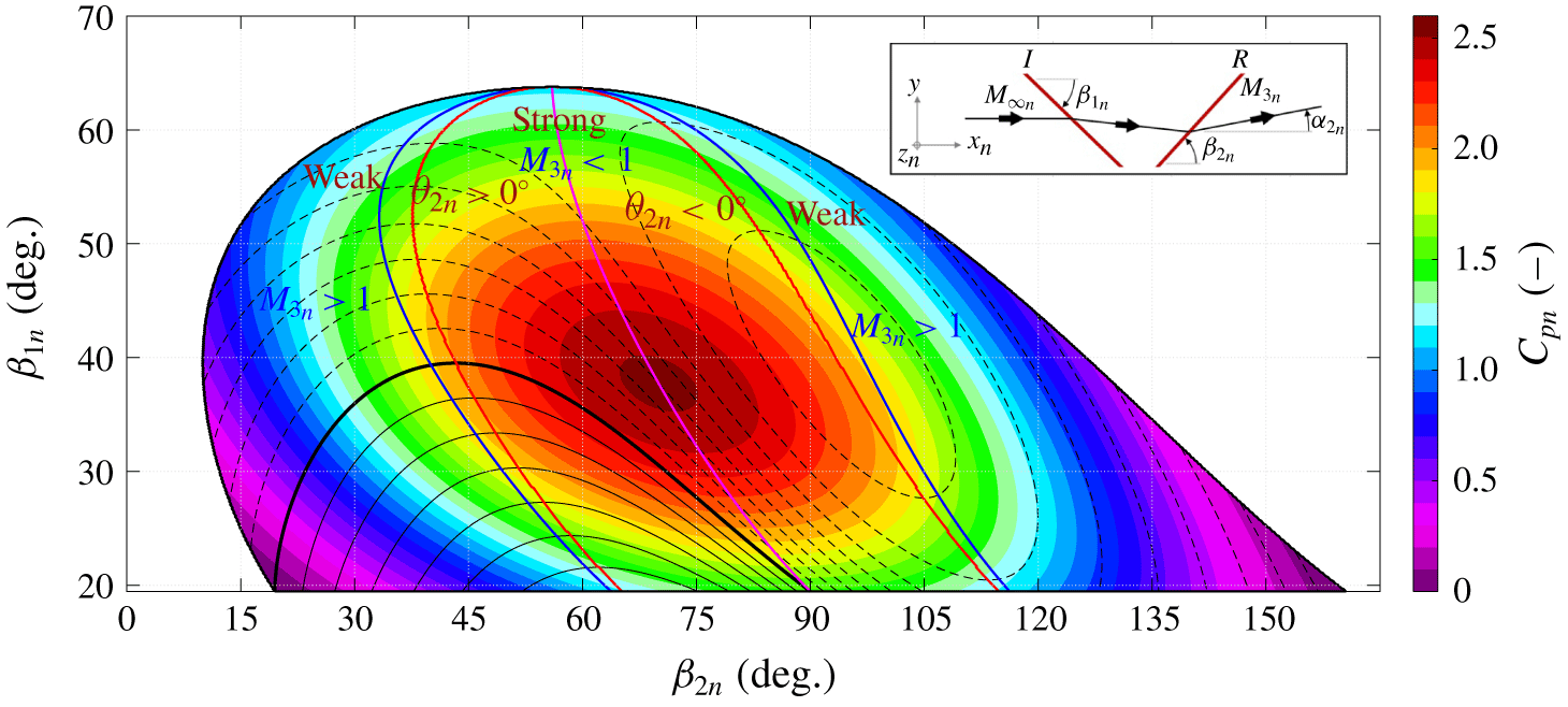
The pressure rise coefficient has been demonstrated in two-dimensional flows as an effective strength parameter for scaling separated turbulent interactions (Morgan et al. Reference Morgan, Duraisamy, Nguyen, Kawai and Lele2013; Souverein et al. Reference Souverein, Bakker and Dupont2013). In addition to affecting the scale of interactions, this parameter can also significantly influence the onset of unsteadiness within transitional SBLIs (Sansica, Sandham & Hu Reference Sansica, Sandham and Hu2016; Sivasubramanian & Fasel Reference Sivasubramanian and Fasel2016). The pressure rise coefficient equates to the interaction pressure rise normalised by the incoming flow dynamic pressure. Once extended to the  $x_{n}$–
 $y$ plane (as discussed prior) this returns equation (4.1).
 $$\begin{eqnarray}{C_{p}}_{n}=\frac{p_{post}-p_{pre}}{q_{\infty }\cos ^{2}\unicode[STIX]{x1D713}}=\frac{2}{\unicode[STIX]{x1D6FE}M_{\infty }^{2}\cos ^{2}\unicode[STIX]{x1D713}}\left(\frac{p_{post}}{p_{pre}}-1\right).\end{eqnarray}$$
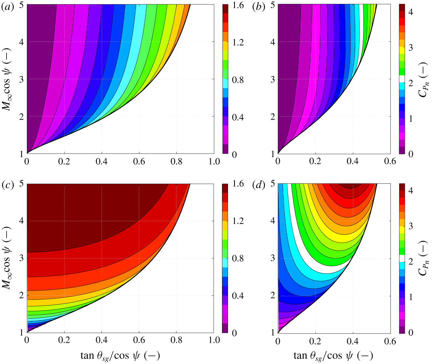
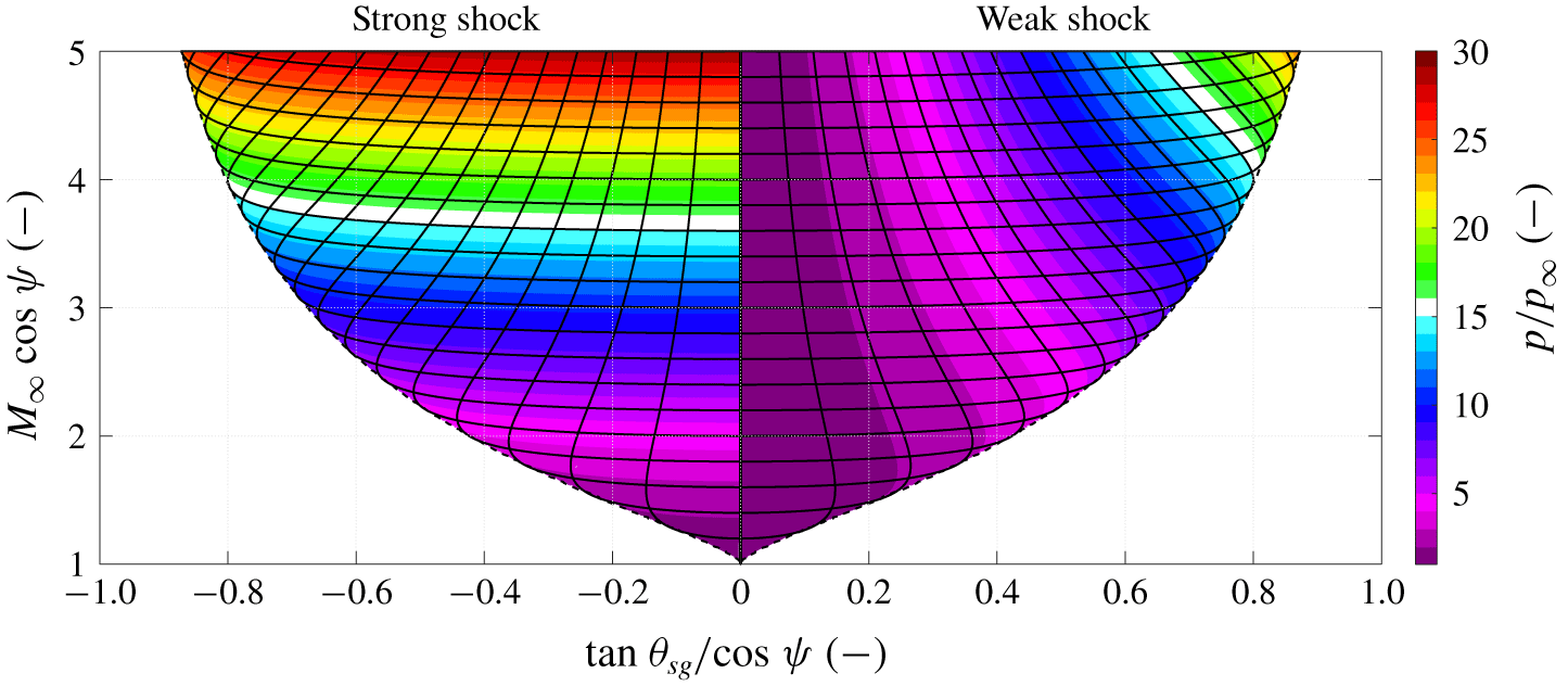
The pressure rise coefficients for a range of shock systems are shown in figure 8. Single-shock systems representing weak and strong solutions are shown in figure 8(a) and figure 8(c), respectively. Dual-shock systems representing weak–weak and weak–strong are shown in figure 8(b) and figure 8(d), respectively.
Typical swept compression ramp conditions are given directly by the weak solution (see figure 8a) where the interaction strength increases as: (i) Mach number ( $M_{\infty }$) is decreased, (ii)
 $x$–
 $y$ plane ramp deflection angle (
 $\unicode[STIX]{x1D703}_{sg}$) is increased or (iii) sweep angle (
 $\unicode[STIX]{x1D713}$) is increased. The free-stream strength of swept sharp-fin shocks can also be determined using this figure, providing the reference frame is considered such that the
 $x$–
 $y$ plane shock generator angle
 $\unicode[STIX]{x1D703}$ is defined in a plane perpendicular to the swept plane.
Normalised pressure rise coefficient across various shock systems. (a,c) Represent conditions across a single shock, (b,d) represent conditions across a shock reflection where the first shock is a weak shock. (a,b) Feature systems with a weak final shock, (c,d) feature systems with a strong final shock. The shock detachment boundary is shown by a solid black line. Note, the colour scale differs between each column. (a) Weak incident shock. (b) Weak–weak shock reflection. (c) Strong incident shock. (d) Weak–strong shock reflection.

Alternatively, one can also refer to the strong solution data in figure 8(c) by considering the equivalences between shock geometries (Domel Reference Domel2016). For example, an unswept sharp-fin shock could be defined with the weak solution data using a sweep angle of  $\unicode[STIX]{x1D713}$ and
 $x$–
 $y$ plane shock generator angle
 $\unicode[STIX]{x1D703}$. It could also be defined in a reference frame perpendicular to this such that sweep is given by
 $\unicode[STIX]{x1D713}=90^{\circ }-\unicode[STIX]{x1D6FD}$ and the new
 $x$–
 $y$ plane shock generator angle is
 $0^{\circ }$. In this new reference frame the two solutions correspond to a Mach wave (weak solution) or an oblique shock (strong solution). The strong shock produces an inverse trend compared to the weak case. Namely, the strength now decreases as: (i) Mach number (
 $M_{\infty }$) is decreased, (ii)
 $x$–
 $y$ plane ramp deflection angle (
 $\unicode[STIX]{x1D703}_{sg}$) is increased or (iii) sweep angle (
 $\unicode[STIX]{x1D713}$) is increased.
Figure 8(b) describes the pressure rise across two weak reflected shocks, which forms the main focus of this study. As found previously, shock generator angles are more limited in the two-shock system resulting in a smaller envelope of permissible conditions that will result in attached shocks. At high Mach numbers and/or low sweep angles, the interaction becomes largely insensitive to both Mach number and sweep (owing to small angle approximations) and is therefore primarily governed by the  $x$–
 $y$ plane shock generator deflection angle. This implies that in these conditions there is minimal spanwise deflection of the flow and it therefore behaves in a quasi-2-D manner. However, at low Mach numbers and/or moderate to high sweep angle, such a simplification is not viable. Qualitatively, the response agrees with that of a single weak shock (see figure 8a) where the interaction increases in strength for: (i) decreased free-stream Mach number, (ii) increased sweep or (iii) increased
 $x$–
 $y$ plane shock generator deflection angle. Disregarding any of these effects when scaling the strength of an SBLI may result in misinterpretation of fundamental mechanisms present. The weak–strong two-shock system is shown in figure 8(d) for completeness.
The pressure rise coefficient has been used in unswept turbulent SBLIs to characterise the onset of flow separation. By establishing an empirical database of such experiments Souverein et al. (Reference Souverein, Bakker and Dupont2013) demonstrated that the onset of fully separated flow existed when  ${C_{p}}_{n}>0.33$ (for low Reynolds number flows, where
 $Re_{\unicode[STIX]{x1D703}}<10^{4}$), or
 ${C_{p}}_{n}>0.40$ (for high Reynolds number flows, where
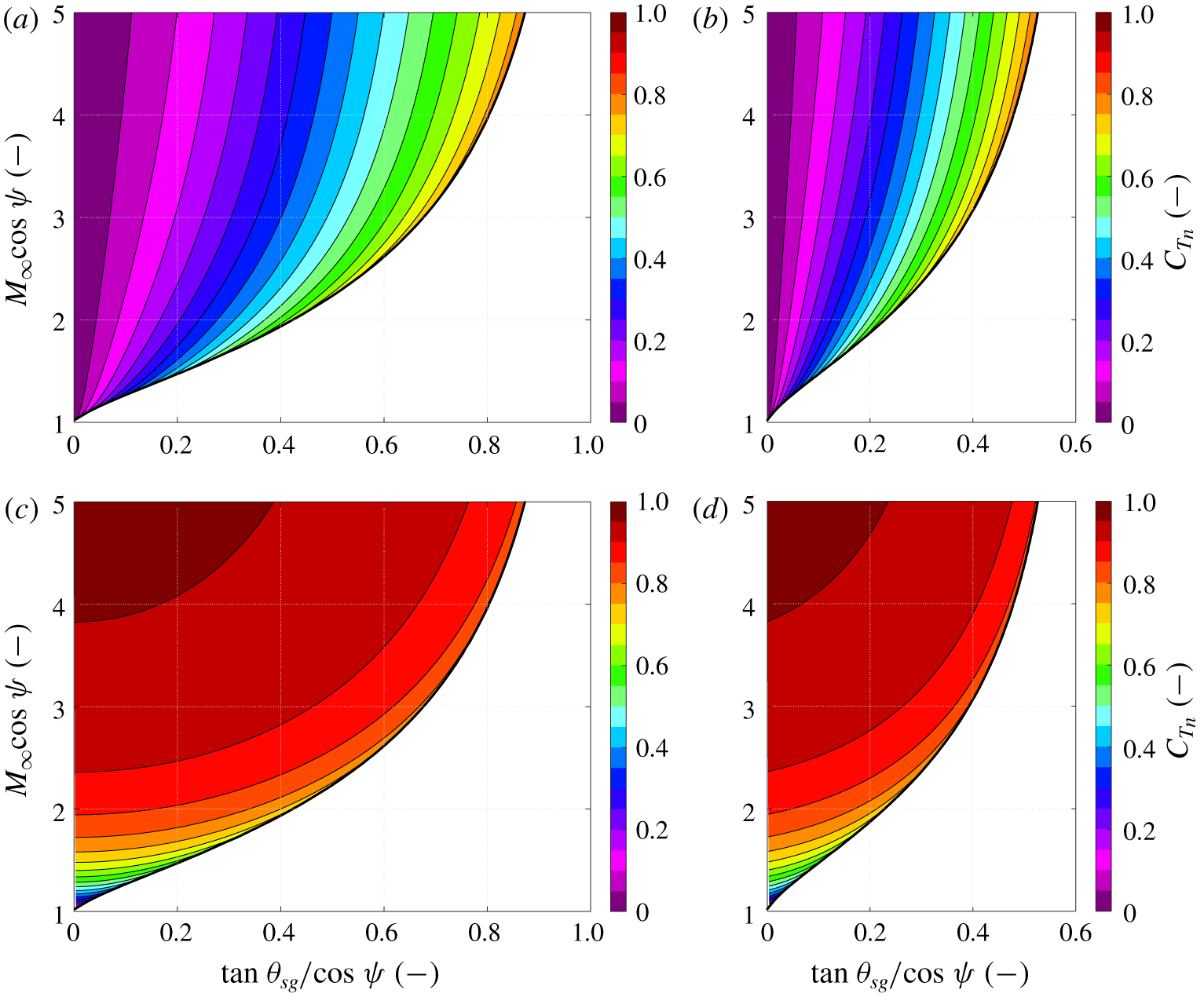
 $Re_{\unicode[STIX]{x1D703}}>10^{4}$). A similar normalised approach may be taken to assess Mach number variation across the shock structure by proposing an equivalent temperature rise coefficient. Equation (4.2) normalises the dimensional temperature rise across a shock structure by the difference between stagnation and the local static temperature measured normal to the sweep (i.e. local dynamic temperature). When used in conjunction with (2.14), this returns an assessment of Mach number throughout the shock reflection, reduced into the two-parameter domain as discussed previously (see (4.3)).
 $$\begin{eqnarray}\displaystyle & \displaystyle {C_{T}}_{n}=\frac{T_{post}-T_{pre}}{\left(T_{0}-T_{\infty }\right)\cos ^{2}\unicode[STIX]{x1D713}}=\frac{2}{\left(\unicode[STIX]{x1D6FE}-1\right)M_{\infty }^{2}\cos ^{2}\unicode[STIX]{x1D713}}\left(\frac{T_{post}}{T_{pre}}-1\right), & \displaystyle\end{eqnarray}$$
 $$\begin{eqnarray}\displaystyle & \displaystyle M^{2}=\frac{2M_{\infty }^{2}(1-C_{Tn}\cos ^{2}\unicode[STIX]{x1D713})}{2+(\unicode[STIX]{x1D6FE}-1)C_{Tn}M_{\infty }^{2}\cos ^{2}\unicode[STIX]{x1D713}}. & \displaystyle\end{eqnarray}$$
Normalised temperature rise coefficient across various shock systems. (a,c) Represent conditions across a single shock, (b,d) represent conditions across a shock reflection where the first shock is a weak shock (required to induce a second shock). (a,b) Feature systems with a weak final shock, (c,d) feature systems with a strong final shock. The shock detachment boundary is shown by a solid black line. (a) Weak incident shock. (b) Weak–weak shock reflection. (c) Strong incident shock. (d) Weak–strong shock reflection.

Demonstration of this temperature rise coefficient is shown in figure 9. Results are dominated by the strength of the final shock, such that a strong final shock produces high temperature coefficients (indicating slower flow) which increase with incoming Mach number and induced flow deflection (in  $x_{n}$–
 $y$ plane). Weak-only shock systems produces notably smaller temperature coefficients, although qualitatively retain a similar behaviour.
Finally, one can use (2.14) again to return an alternative formulation for the downstream sideslip angle  $\unicode[STIX]{x1D702}$. The temperature ratio
 $T/T_{\infty }$ is constant regardless of the reference frame in which Mach number is determined. One can use this feature to rewrite this expression as (4.4).
 $$\begin{eqnarray}\frac{T}{T_{\infty }}=\frac{2+(\unicode[STIX]{x1D6FE}-1)M_{\infty }^{2}\cos ^{2}\unicode[STIX]{x1D713}}{2+(\unicode[STIX]{x1D6FE}-1)M_{n}^{2}}.\end{eqnarray}$$
Equation (4.5) defines the relationship between the Mach number measured normal to the sweep and the absolute local Mach number for a given flow deflection. Using (4.4) to return  $M_{n}$ and (4.2) to substitute
 ${C_{T}}_{n}$, this may be written as (4.6) and then employed to calculate the downstream sideslip angle
 $\unicode[STIX]{x1D702}$. This presents as an alternate formulation of (2.17). Since the terms for temperature coefficient
 ${C_{T}}_{n}$ and
 $x_{n}$–
 $y$ plane deflection angle
 $\unicode[STIX]{x1D6FC}_{n}$ both collapse in the two-variable domain, one can use this equation to determine the sideslip angle
 $\unicode[STIX]{x1D702}$ for a given shock solution with a defined swept angle
 $\unicode[STIX]{x1D713}$.
 $$\begin{eqnarray}\displaystyle & \displaystyle \frac{M^{2}}{M_{n}^{2}}=\sin ^{2}\unicode[STIX]{x1D6FC}_{n}+\frac{\cos ^{2}\unicode[STIX]{x1D6FC}_{n}}{\cos ^{2}(\unicode[STIX]{x1D713}+\unicode[STIX]{x1D702})}, & \displaystyle\end{eqnarray}$$
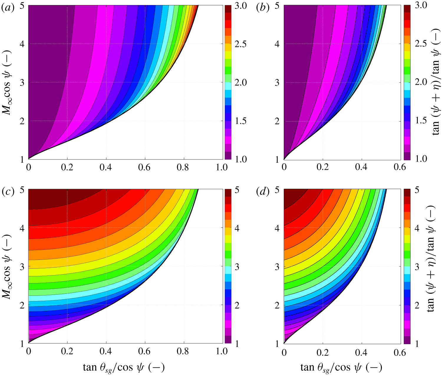
 $$\begin{eqnarray}\displaystyle & \displaystyle \frac{\tan (\unicode[STIX]{x1D713}+\unicode[STIX]{x1D702})}{\tan \unicode[STIX]{x1D713}}=\frac{1}{\cos \unicode[STIX]{x1D6FC}_{n}\sqrt{1-C_{Tn}}}. & \displaystyle\end{eqnarray}$$
The relation  $\tan (\unicode[STIX]{x1D713}+\unicode[STIX]{x1D702})/\text{tan}\,\unicode[STIX]{x1D713}$ can therefore be considered as the appropriate term for the normalised spanwise flow deflection, as shown in figure 10. For a given shock generator sweep, the sideslip deflection is observed to be greater for the weak–weak shock reflection when compared to the single weak shock. Both cases experience increased sideslip for increased shock generator deflection angles and decreased free-stream Mach numbers. Strong shocks significantly increase sideslip deflection over the weak shock counterparts. In this case, trends with shock generator deflection angle and Mach number invert. Also, sideslip is reduced for increased shock generator deflection angles and decreased free-stream Mach numbers.
Normalised sideslip across various shock systems. (a,c) Represent conditions across single shock, (b,d) represent conditions across dual-shock reflection systems where the first shock is a weak shock. (a,b) Feature systems with a weak final shock, (c,d) feature systems with a strong final shock. The shock detachment boundary is shown by a solid black line. Note, the colour scale differs between each row. (a) Weak incident shock. (b) Weak–weak shock reflection. (c) Strong incident shock. (d) Weak–Strong shock reflection.

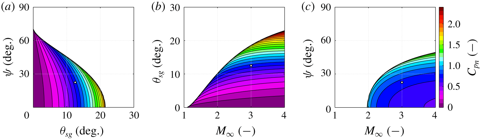
Attention is now returned to the three-parameter domain to demonstrate the effect of modifications to a given shock reflection environment. A nominal flow field is defined using a shock generator with  $\unicode[STIX]{x1D713}=22.5^{\circ }$ and
 $\unicode[STIX]{x1D703}_{sg}=12.5^{\circ }$ in Mach 3.0 flow. Figure 11 demonstrates the influence of these parameters with respect to the pressure rise coefficient
 ${C_{p}}_{n}$ (as defined by (4.1)). Inspection of the data suggests that the normalised pressure rise is most sensitive to changes in shock generator deflection angle. The effect of sweep and Mach number appear to be less significant, a feature clearly evident on the broad bands in figure 11(c). By considering each parameter independently, one can establish the following partial derivatives at the nominal condition defined above (
 $\unicode[STIX]{x1D713}=22.5^{\circ }$,
 $\unicode[STIX]{x1D703}_{sg}=12.5^{\circ }$,
 $M_{\infty }=3.0$). This determines the relative influence on the interaction pressure rise:
 $\unicode[STIX]{x2202}{C_{p}}_{n}/\unicode[STIX]{x2202}\unicode[STIX]{x1D713}=0.0121~\text{deg}^{-1}$,
 $\unicode[STIX]{x2202}{C_{p}}_{n}/\unicode[STIX]{x2202}\unicode[STIX]{x1D703}_{sg}=0.102~\text{deg}^{-1}$ and
 $\unicode[STIX]{x2202}{C_{p}}_{n}/\unicode[STIX]{x2202}M_{\infty }=-0.146$. This approach can be followed for any arbitrary configurations.
Influence of sweep angle, deflection angle and Mach number on the pressure rise across a weak–weak shock reflection. Nominal case is for a  $\unicode[STIX]{x1D713}=22.5^{\circ }$
 $\unicode[STIX]{x1D703}_{sg}=12.5^{\circ }$ shock generator in Mach 3.0 flow (indicated by the circle marker). Each panel demonstrates the effect of varying two parameters while keeping the third constant. (a) Constant Mach number (
 $M_{\infty }=3.0$). (b) Constant
 $x$–
 $z$ plane sweep angle (
 $\unicode[STIX]{x1D713}=22.5^{\circ }$). (c) Constant
 $x$–
 $y$ plane deflection angle (
 $\unicode[STIX]{x1D703}_{sg}=12.5^{\circ }$).

4.4 Comparisons to other interaction types
Flow under swept shock generators can be considered identical to that over an inverted inviscid swept compression ramp. Both configurations experience flow deflection routinely defined in the  $x$–
 $y$ plane normal to the swept plane, and therefore can be contrasted directly. As such, results from the model measured across the incident shock agree with prior compression ramp-specific models that have been presented (Settles & Teng Reference Settles and Teng1984; Domel Reference Domel2016). The present model expands upon this knowledge and characterises the shock reflection against a wall parallel to the shock generator.
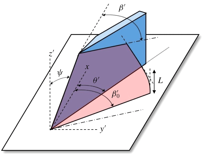
Comparisons with other supersonic deflected flow configurations can also be made, but consideration of the reference frame is vital. To illustrate this one may consider the swept sharp-fin configuration, as shown in figure 12, which is similar to the shock structure at the root plane of a swept impinging oblique SBLI. Prior research has characterised the shock structure and surface topology beneath the fin (Settles & Lu Reference Settles and Lu1985). Away from the wall, the shock develops at a consistent angle; however, near to the wall, the shock is shallower. This near-wall behaviour matches similar observations at the root of a swept impinging oblique SBLIs (Threadgill et al. Reference Threadgill, Stab, Doehrmann and Little2017), and in analogous delta-wing flows (Fowell Reference Fowell1956; Squire Reference Squire1968). A state of equivalence between these flows can be made since each configuration demonstrates highly swept oblique shocks interacting with non-porous plane. However, a crucial difference between these configurations is in the definition of the shock generator geometries which needs to be understood to enable comparison.
Schematic diagram of shock structure in inviscid flow past a swept sharp fin (adapted from Settles & Lu Reference Settles and Lu1985).  $L$ represents an inviscid inception length, characterising the spanwise extent of the curved root shock.

The swept sharp fin in figure 12 is essentially a flat plate with a swept sharp leading edge mounted normal to the wall at an incidence to the incoming flow (Settles & Lu Reference Settles and Lu1985). By this definition, the leading edge is not in the  $x$–
 $z^{\prime }$ plane, but at a plane rotated around the
 $z^{\prime }$ axis by an angle
 $\unicode[STIX]{x1D703}^{\prime }$. Figure 13 demonstrates the implication of this when compared to the swept shock generator and compression ramp definitions discussed previously. The leading edge is held constant between the two configurations, producing a difference in the wall location at the base of the shock due to rotation around the
 $z$-axis of
 $\unicode[STIX]{x1D709}$, characterised by (4.7).
Since inviscid conditions collapse well in the shock generator  $x-y-z$ reference frame, it is desirable to transform the swept sharp-fin geometry into a swept impinging oblique shock generator such that a similar analysis can be followed. The effect of this reference frame transformation is that the sharp fin sweep and deflection angles are no longer equal to that defined for the effective 2-D shock generator. Instead, equations (4.8) and (4.9) are used to redefine these variables, respectively.
 $$\begin{eqnarray}\displaystyle & \displaystyle \tan \unicode[STIX]{x1D709}=\tan \unicode[STIX]{x1D713}^{\prime }\sin \unicode[STIX]{x1D703}^{\prime }, & \displaystyle\end{eqnarray}$$
 $$\begin{eqnarray}\displaystyle & \displaystyle \tan \unicode[STIX]{x1D713}=\tan \unicode[STIX]{x1D713}^{\prime }\cos \unicode[STIX]{x1D703}^{\prime }\cos \unicode[STIX]{x1D709}, & \displaystyle\end{eqnarray}$$
 $$\begin{eqnarray}\displaystyle & \displaystyle \tan \unicode[STIX]{x1D703}_{sg}=\tan \unicode[STIX]{x1D709}/\tan \unicode[STIX]{x1D713}. & \displaystyle\end{eqnarray}$$
An  $y$–
 $z$ plane comparison between swept sharp-fin and shock reflections. The reference frame for the swept sharp-fin flow is given by the
 $x$,
 $y^{\prime }$ and
 $z^{\prime }$ vectors.

Understanding the differences between these geometries is vital when comparing data from swept SBLIs induced by various geometries. A focus of this article is the collapse of data with appropriate consideration of the sweep. A similar collapse of inviscid swept sharp-fin data requires substitution of appropriate terms into the abscissa and ordinate definitions from figure 8. Equations (4.10) and (4.11) give the appropriate relations, written in terms of the sharp-fin geometry definition.
 $$\begin{eqnarray}\displaystyle & \displaystyle \cos \unicode[STIX]{x1D713}=\cos \unicode[STIX]{x1D713}^{\prime }\sqrt{\tan ^{2}\unicode[STIX]{x1D713}^{\prime }\sin ^{2}\unicode[STIX]{x1D703}^{\prime }+1}, & \displaystyle\end{eqnarray}$$
 $$\begin{eqnarray}\displaystyle & \displaystyle \tan \unicode[STIX]{x1D703}_{sg}=\tan \unicode[STIX]{x1D703}^{\prime }\sqrt{\tan ^{2}\unicode[STIX]{x1D713}^{\prime }\sin ^{2}\unicode[STIX]{x1D703}^{\prime }+1}. & \displaystyle\end{eqnarray}$$
It is clear that terms cancel when defining the abscissa variable, such that  $\tan \unicode[STIX]{x1D703}^{\prime }/\text{cos}\,\unicode[STIX]{x1D713}^{\prime }=\tan \unicode[STIX]{x1D703}_{sg}/\text{cos}\,\unicode[STIX]{x1D713}$. However, the ordinate variable must now include the effect of deflection angle in addition to sweep, such that it is defined as
 $M_{\infty }\cos \unicode[STIX]{x1D713}^{\prime }\sqrt{\tan ^{2}\unicode[STIX]{x1D713}^{\prime }\sin ^{2}\unicode[STIX]{x1D703}^{\prime }+1}$, which equates to
 $M_{\infty }\cos \unicode[STIX]{x1D713}^{\prime }/\text{cos}\,\unicode[STIX]{x1D709}$, if (4.7) is utilised.
4.5 Shock structure at the root
Typical impinging shocks experienced outside of fundamental research environments are unlikely to be induced where the domain spanwise boundary planes are aligned with downstream sideslip angles so as to prevent influencing the inviscid shock. It is therefore important to gain an understanding of the broader environment in which such an effect is experienced.
Impinging oblique SBLIs are commonly induced by a shock generating surface located away from the wall. When swept, a spanwise component of velocity is induced. If a slip plane is introduced to the fluid that restricts such flow (i.e. sidewalls of a engine inlet, or symmetry plane beneath delta wing) this could induce either a secondary compression (forming a shock reflection) or a local expansion region, depending on the inclination of the fluid to the plane (Squire Reference Squire1968). In the former case, the reflected shock can be solved directly using the inviscid model presented above, providing the appropriate reference frame is considered and the shock is attached. However, determination of latter case that exhibits local expansion and acceleration of the fluid is significantly more challenging and is addressed below.
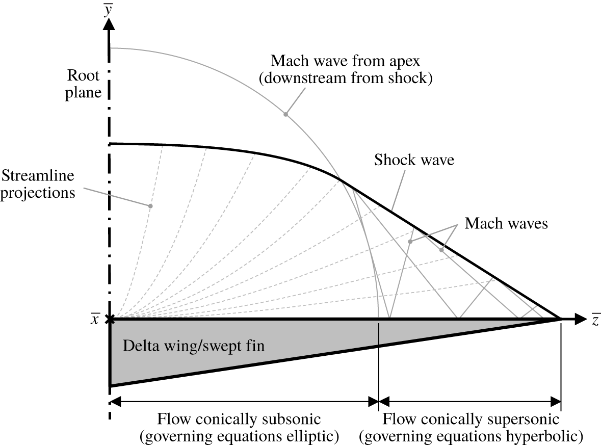
A commonly studied configuration which exhibits this behaviour is flow near the centreline beneath a delta-wing model. The local expansion acts to relieve the downstream flow deflection requirements, weakening the shock, and moving the shock–wall impingement location further downstream. This is shown schematically in figure 12 for an inviscid swept sharp-fin configuration which is identical to the delta-wing flow (albeit split at the centreline symmetry plane). Figure 14 shows how the outboard region of the flow is conically supersonic, equal to the uniform flow predicted by the present inviscid model. The central region is conically subsonic and bound by the Mach wave emanating from flow at the apex.
Schematic showing curved shock region near the root plane (adapted from Roe (Reference Roe1970) and Babaev (Reference Babaev1963)).

The solution for the shock shape and downstream flow conditions in this region is not directly solvable (Settles & Lu Reference Settles and Lu1985). Various numerical solutions have been proposed (Babaev Reference Babaev1963; Squire Reference Squire1968; Voskresenskii Reference Voskresenskii1968). In addition, several simplified models of this region have been created (Hayes & Probstein Reference Hayes and Probstein1959; Roe Reference Roe1970; Woods Reference Woods1970). However, their suitability in modelling shock shape at moderate Mach numbers is generally poor as they rely on assumptions proposed to address hypersonic flows (Messiter Reference Messiter1963). Messiter (Reference Messiter1963) scales the dimensional variables using  $\unicode[STIX]{x1D700}$, defined as the inverse density ratio across an equivalent unswept shock (i.e.
 $\unicode[STIX]{x1D700}=\unicode[STIX]{x1D70C}_{1}/\unicode[STIX]{x1D70C}_{2}$, see (4.12)). As the shock attitude is not known a priori it is assumed to be parallel to the unswept shock generator surface (
 $\unicode[STIX]{x1D6FD}^{\prime }=\unicode[STIX]{x1D703}^{\prime }$) inclined to the flow running parallel to the shock generator surface, a reasonable assumption in hypersonic flows with significant flow deflection.
 $$\begin{eqnarray}\displaystyle \unicode[STIX]{x1D700}=\frac{\unicode[STIX]{x1D70C}_{\infty }}{\unicode[STIX]{x1D70C}}=\frac{\unicode[STIX]{x1D6FE}-1}{\unicode[STIX]{x1D6FE}+1}+\frac{2}{\left(\unicode[STIX]{x1D6FE}+1\right)M_{\infty }^{2}\sin ^{2}\unicode[STIX]{x1D703}^{\prime }}. & & \displaystyle\end{eqnarray}$$
Dimensional terms are normalised using  $\unicode[STIX]{x1D700}$ in (4.13), (4.14), (4.15) and (4.16). The terms noted with a bar accent (e.g.
 $\bar{x}$) are dimensional and defined in a reference frame rotated around the
 $z^{\prime }$ axis, such that the
 $\bar{x}$ axis runs parallel to the shock generator surface with the origin at the generator apex. The spanwise extent of the shock generator is normalised using (4.14) to define
 ${\check{z}}=\unicode[STIX]{x1D6FA}$ when
 $z/\bar{x}=b$, such that
 ${\check{z}}$ varies between 0 at the central plane to
 $\unicode[STIX]{x1D6FA}$ at the tip.
 $$\begin{eqnarray}\displaystyle & \displaystyle \check{y}=\frac{\bar{y}/\bar{x}}{\unicode[STIX]{x1D700}\tan \unicode[STIX]{x1D703}^{\prime }}, & \displaystyle\end{eqnarray}$$
 $$\begin{eqnarray}\displaystyle & \displaystyle {\check{z}}=\frac{\bar{z}/\bar{x}}{\unicode[STIX]{x1D700}^{1/2}\tan \unicode[STIX]{x1D703}^{\prime }}, & \displaystyle\end{eqnarray}$$
 $$\begin{eqnarray}\displaystyle & \displaystyle \check{w}=\frac{w}{\unicode[STIX]{x1D700}^{1/2}U_{\infty }\sin \unicode[STIX]{x1D703}^{\prime }}, & \displaystyle\end{eqnarray}$$
 $$\begin{eqnarray}\displaystyle & \displaystyle \check{p}=\frac{1}{\unicode[STIX]{x1D700}}\left[\frac{p-p_{\infty }}{\unicode[STIX]{x1D70C}_{\infty }U_{\infty }^{2}\sin ^{2}\unicode[STIX]{x1D703}^{\prime }}-1\right]=\frac{1}{\unicode[STIX]{x1D700}}\left[\frac{C_{p}}{\sin ^{2}\unicode[STIX]{x1D703}^{\prime }}-1\right]. & \displaystyle\end{eqnarray}$$
At high Mach numbers and significant flow deflections,  $\unicode[STIX]{x1D700}$ tends towards
 $(\unicode[STIX]{x1D6FE}-1)/(\unicode[STIX]{x1D6FE}+1)$ and closely resembles conditions downstream of a real shock over a matching wedge. However, at low Mach numbers and small flow deflections the disparity between this estimation and the real flow can be striking, resulting in significant errors when estimating shock shape and strength (Squire Reference Squire1968; Roe Reference Roe1970).
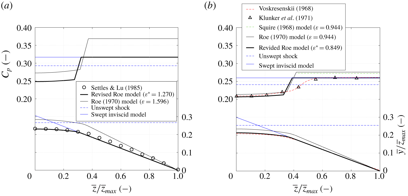
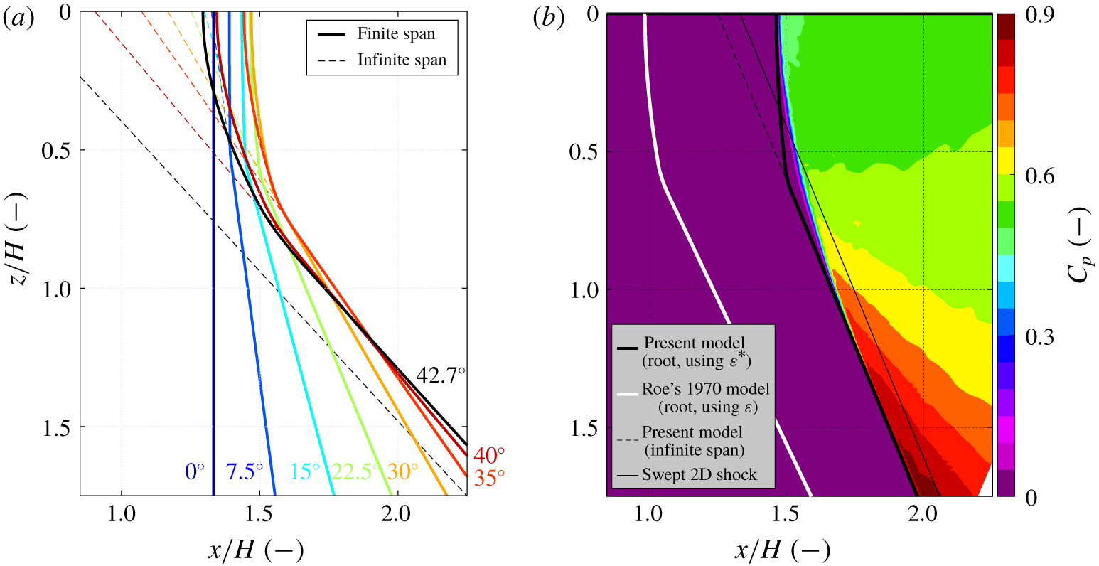
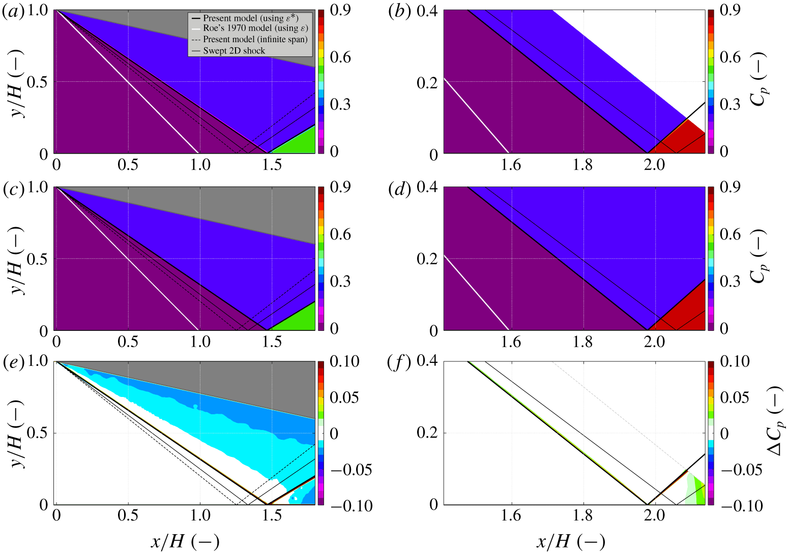
Roe’s (Reference Roe1970) delta-wing-induced shock estimation is attractive as the solution is continuous, derived from the equations of motion, and relies on simple formulation. A summary of the approach is provided below, but the reader is directed to the source papers for full details of derivation (Messiter Reference Messiter1963; Roe Reference Roe1970). Employing Messiter’s (Reference Messiter1963) non-dimensionalisation approach with  $\unicode[STIX]{x1D700}$ (returning
 $\check{y}$ and
 ${\check{z}}$, etc.), Roe reduces the shock structure to three zones: (i) uniform outer flow with gradient
 $\text{d}\check{y}/\text{d}{\check{z}}=w_{0}$, (ii) intermediate parabolic blending region and (iii) parabolic central region with zero gradient at
 ${\check{z}}=0$.
 $$\begin{eqnarray}\left.\begin{array}{@{}rll@{}}\displaystyle (\text{i}) & \check{y}_{s}=-\check{w}_{0}\left({\check{z}}-\unicode[STIX]{x1D6FA}\right), & 1+\check{w}_{0}\leqslant {\check{z}}\leqslant \unicode[STIX]{x1D6FA},\\ \displaystyle (\text{ii}) & \check{y}_{s}=1-\check{w}_{0}+{\displaystyle \frac{\check{w}_{0}^{2}}{2}}-{\displaystyle \frac{\left({\check{z}}-1\right)^{2}}{2}}, & 1+\check{w}_{1}\leqslant {\check{z}}<1+\check{w}_{0},\\ \displaystyle (\text{iii}) & \check{y}_{s}=1-\check{w}_{0}+{\displaystyle \frac{\check{w}_{0}^{2}}{2}}+{\displaystyle \frac{\check{w}_{1}}{2}}-{\displaystyle \frac{\check{w}_{1}}{1+\check{w}_{1}}}{\displaystyle \frac{{\check{z}}^{2}}{2}}, & 0\leqslant {\check{z}}<1+\check{w}_{1}.\end{array}\right\}\end{eqnarray}$$
The terms  $\check{w}_{0}$ and
 $\check{w}_{1}$ represent non-dimensionalised spanwise velocities and are determined using (4.18) and (4.19). They also act to define the matching points between the three curves listed above defining the shock shape, such that the central curved shock region is bound by
 ${\check{z}}=1+\check{w}_{1}$ and the outer uniform shock region is bound by
 ${\check{z}}=1+\check{w}_{0}$. Solving (4.18) for
 $\check{w}_{0}$ also reveals further significance of the spanwise term
 $\unicode[STIX]{x1D6FA}$, where if it has a value less than 2 there is no solution and the shock is fully detached across the entire span.
 $$\begin{eqnarray}\displaystyle & \displaystyle \unicode[STIX]{x1D6FA}=\frac{\check{w}_{0}^{2}+1}{w_{0}}, & \displaystyle\end{eqnarray}$$
 $$\begin{eqnarray}\displaystyle & \displaystyle \left(1+w_{1}\right)^{2}=1+3\check{w}_{0}^{2}-2\check{w}_{0}^{3}. & \displaystyle\end{eqnarray}$$
Finally, the shock structure is transformed back to the upstream-aligned reference frame using (4.20) and (4.21).
 $$\begin{eqnarray}\displaystyle & \displaystyle \frac{y_{s}^{\prime }}{x}=\frac{\tan \unicode[STIX]{x1D703}^{\prime }+\bar{y}/\bar{x}}{1-\left(\bar{y}/\bar{x}\right)\tan \unicode[STIX]{x1D703}^{\prime }}, & \displaystyle\end{eqnarray}$$
 $$\begin{eqnarray}\displaystyle & \displaystyle \frac{z^{\prime }}{x}=\frac{\bar{z}/\bar{x}}{\cos \unicode[STIX]{x1D703}^{\prime }-\left(\bar{y}/\bar{x}\right)\sin \unicode[STIX]{x1D703}^{\prime }}. & \displaystyle\end{eqnarray}$$
In a similar manner, the model also returns estimation of the non-dimensionalised pressure downstream of the shock using (4.22).
 $$\begin{eqnarray}\left.\begin{array}{@{}rll@{}}\displaystyle \text{(i)} & \check{p}=1+{\displaystyle \frac{\check{w}_{0}^{2}}{2}} & 1+\check{w}_{0}\leqslant {\check{z}}\leqslant \unicode[STIX]{x1D6FA},\\ \text{(ii)} & \check{p}=1+{\displaystyle \frac{\check{w}_{0}^{2}}{2}}+2\left({\check{z}}-1-\check{w}_{0}\right) & 1+\check{w}_{1}\leqslant {\check{z}}<1+\check{w}_{0},\\ \text{(iii)} & \check{p}=A+B\check{y}^{2} & 0\leqslant {\check{z}}<1+\check{w}_{1},\end{array}\right\}\end{eqnarray}$$
where the terms  $A$ and
 $B$ are given by (4.23) and (4.24), respectively.
 $$\begin{eqnarray}\displaystyle & \displaystyle A=\left(1-w_{0}^{2}\right)+\frac{w_{1}}{2}\left(6w_{1}^{2}+9w_{1}+4\right)+3w_{1}^{2}\left(1+w_{1}\right)^{2}\log \left(\frac{w_{1}}{1+w_{1}}\right), & \displaystyle\end{eqnarray}$$
 $$\begin{eqnarray}\displaystyle & \displaystyle B=-3w_{1}\left[\frac{1}{\left(1+w_{1}\right)}+\frac{1}{2\left(1+w_{1}\right)^{2}}+\log \left(\frac{w_{1}}{1+w_{1}}\right)\right]. & \displaystyle\end{eqnarray}$$
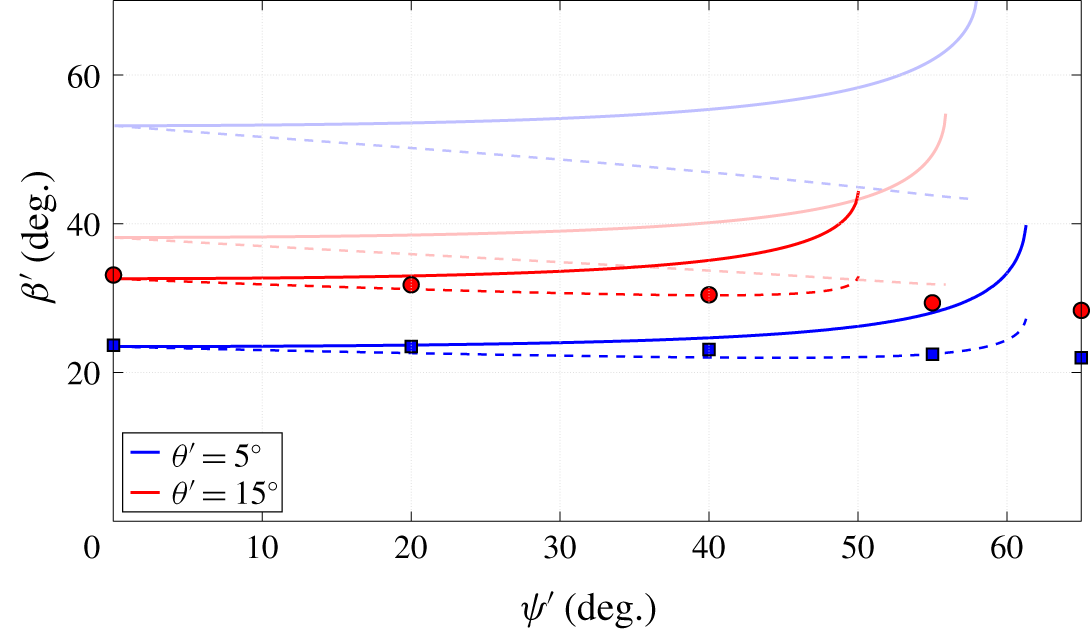
While the model offers useful estimation of the induced shock shape and strength, there are notable discrepancies at low Mach numbers and strong flow deflections (Roe Reference Roe1970). Comparison to such experimental data is shown in figure 15 for various delta-wing geometries in  $M_{\infty }=2.95$ flow (Settles & Lu Reference Settles and Lu1985). The experimental centreline shock angle is derived from schlieren imaging and compared to the theoretical value determined from Roe’s model using
 $\tan \unicode[STIX]{x1D6FD}_{0}^{\prime }=y_{s}^{\prime }/x$ (at
 $z^{\prime }=0$). Significant differences are observed between the data which appear to become worse as the deflection angle is reduced (consistent with strengthening invalidity of assumptions when defining
 $\unicode[STIX]{x1D700}$ as a scaling variable).
Shock angles for Mach 2.95 delta-wing experiment (Settles & Lu Reference Settles and Lu1985). Markers indicate experimental data for the root shock angle, from Settles & Lu (Reference Settles and Lu1985). Solid and dashed bold lines indicate the inviscid quasi-infinite-span shock angle and root shock angle (using  $\unicode[STIX]{x1D700}^{\ast }$), respectively, defined in a matching reference frame away from the wall using the present inviscid model (weak shock solutions plotted, only). Similarly, the corresponding faded solid and dashed lines indicate inviscid shock angles and root shock angles, respectively, with results extracted from Roe’s uncorrected model for the shock structure (using
 $\unicode[STIX]{x1D700}$).

As the uniform outer flow is now directly determined using the inviscid infinite-span model presented in this paper, one can use the resultant shock geometries to define the non-dimensionalised shock gradient  $\check{w}_{0}$ and, in turn, estimate a revised scaling parameter, termed
 $\unicode[STIX]{x1D700}^{\ast }$ for clarity. After some manipulation, this returns (4.25), which replaces the previous definition of
 $\unicode[STIX]{x1D700}$ given in (4.12).
 $$\begin{eqnarray}\unicode[STIX]{x1D700}^{\ast }=\frac{\tan \left(\unicode[STIX]{x1D6FD}^{\prime }-\unicode[STIX]{x1D703}^{\prime }\right)}{\tan \unicode[STIX]{x1D703}^{\prime }}-\tan ^{2}\left(\unicode[STIX]{x1D6FD}^{\prime }-\unicode[STIX]{x1D703}^{\prime }\right)\tan ^{2}\unicode[STIX]{x1D713}^{\prime }.\end{eqnarray}$$
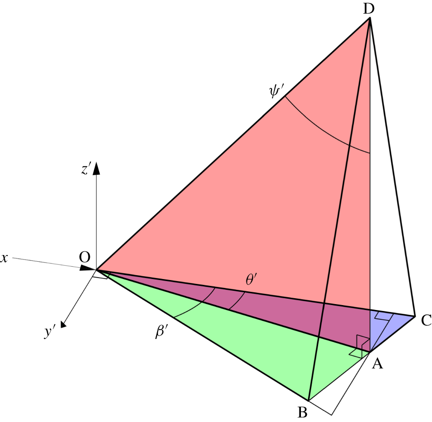
This new term is thus used to normalise dimensional variables following Messiter’s (Reference Messiter1963) approach. Visualised in figure 16, this parameter physically represents  $\unicode[STIX]{x1D700}^{\ast }=(|\boldsymbol{B}|/|\boldsymbol{C}|)-(|\boldsymbol{B}|/|\boldsymbol{D}|)^{2}$ (where each vector is defined relative to vertex
 $A$).
Schematic diagram demonstrating quasi-infinite physical geometries used to define normalisation variable  $\unicode[STIX]{x1D700}^{\ast }$ (to scale for
 $M_{\infty }=2.95$,
 $\unicode[STIX]{x1D713}^{\prime }=40^{\circ }$,
 $\unicode[STIX]{x1D703}^{\prime }=15^{\circ }$).

The revised estimation of root shock shapes for the delta-wing experiments presented in figure 15 shows significant improvement when using  $\unicode[STIX]{x1D700}^{\ast }$ over the previous scaling term
 $\unicode[STIX]{x1D700}$ (plotted lines represent full range of weak shock solutions, from the unswept
 $\unicode[STIX]{x1D713}^{\prime }=0^{\circ }$ case to shock detachment at
 $\unicode[STIX]{x1D713}^{\prime }=\unicode[STIX]{x1D713}_{max}^{\prime }$). The modelled root shock structures become shallower in all cases, closely matching experimental observations at moderate and low angles of sweep. At higher sweep angles (within approximately
 $5^{\circ }$ of shock detachment), some divergence is seen between experimental and modelled root shocks. This divergence is associated with invalid assumptions that guide formation of Roe’s model. As conditions for a detached shock are approached, the curved root shock structure extends over a greater extent of the shock generator span and errors due to imposed assumptions are exacerbated. The quasi-infinite shock model is an analytical solution to the shock relations, but predictions of the root structure remain a simplified model. Thus, errors grow since this model is required to predict a greater extent of the shock shape. Regardless, the error at high sweep is still less than that of the previous uncorrected model in most cases.
In addition, since the present motivation of modelling the root shock structure is to understand the impingement pattern for an attached reflected shock, it follows that the deflection at the shock generator will be significantly below conditions required for a detached impingement shock (see figure 7). Therefore, use of the model correction is justified providing the impinging shock is not close to detachment.
Sample shock structures and downstream pressure profiles are shown in figure 17 compared to various validation datasets. Implementation of the revised scaling approach demonstrates a significant improvement against all other models when predicting the shock structure. Experimental data for the Mach 2.95 shock shape in figure 17(a) were determined by observing Mach waves emanating from a delta-wing model with a notched leading edge (Settles & Lu Reference Settles and Lu1985). Excellent agreement is observed between the experimental data and the revised Roe model in the root region. However, the model predicts a shallower shock in the outer region of the flow. This discrepancy is an experimental artefact due to an oversight when interpreting the schlieren observations of the notch-induced shock ripples. It is assumed that the shock ripples propagate along the shock in a strictly 2-D sense (i.e.  $z=\text{const}.$); however, an infinitesimal notch will produce a Mach wave cone that intersects with the shock in two locations, which are dependent on the shock attitude and the direction and speed of the downstream flow. In this case, the upstream shock ripple extends from the notch towards the root as it is observed further downstream. By assuming this to be within the same spanwise plane as the notch, the shock angle is over-predicted resulting in the over-estimate observed in figure 17(a). The reduction of shock sweep near the root decreases this disparity to zero as the centreline of the delta wing is approached, thus giving more accurate shock estimation in this region.
Application of revised scaling approach for root-limited swept shocks using: (a) experimental (Settles & Lu Reference Settles and Lu1985), and (b) numerical (Voskresenskii Reference Voskresenskii1968; Klunker et al. Reference Klunker, South and Davis1971) reference data. Other shock models are shown for comparison (Squire Reference Squire1968; Roe Reference Roe1970). (a) Experimental validation:  $M=2.95$,
 $\unicode[STIX]{x1D713}^{\prime }=40.0^{\circ }$ and
 $\unicode[STIX]{x1D703}^{\prime }=15.0^{\circ }$. (b) Numerical validation:
 $M=4.0$,
 $\unicode[STIX]{x1D713}^{\prime }=50.0^{\circ }$ and
 $\unicode[STIX]{x1D703}^{\prime }=15.0^{\circ }$.

The shock location is established directly in numerically derived results (Voskresenskii Reference Voskresenskii1968) shown in figure 17(b), and return an excellent matches across the entire shock when compared to the revised model using  $\unicode[STIX]{x1D700}^{\ast }$. Surface pressure coefficients derived from the model agree well with the numerical data (Voskresenskii Reference Voskresenskii1968; Klunker et al. Reference Klunker, South and Davis1971), but fail to fully characterise the smoothing of the spanwise pressure rise as is the case for all proposed models in literature. Regardless, the revised model offers an excellent prediction of the centreline pressure and agrees with the infinite-span results (by definition by using
 $\unicode[STIX]{x1D700}^{\ast }$). Other proposed models (Squire Reference Squire1968; Roe Reference Roe1970) tend to over-predict the steepness of the shock and the associated shock-induced pressure rise.
4.6 Swept shock impingement
The above estimation of the shock shape at a delta-wing root enables prediction of the shape of the impingement line exhibited by a swept impinging oblique shock induced by any given shock generator (providing the resultant shocks remain attached). The procedure is as follows:
(i) The shock generator geometry is transformed into a reference frame such that the generator leading edge is perpendicular to the no-penetration plane delimiting the generator root (
 $\unicode[STIX]{x1D703}_{sg}$, $\unicode[STIX]{x1D713}$, $M_{\infty }$).
(ii) The quasi-infinite swept shock solution is determined using the prescribed model (to return
$\unicode[STIX]{x1D719}$, § 2).(iii) An equivalent shock generator is found that satisfies
$\unicode[STIX]{x1D709}=\unicode[STIX]{x0394}\unicode[STIX]{x1D719}$, such that the leading edge matches a corresponding delta-wing model, and that the root plane is oriented to be coincident with root plane ($\unicode[STIX]{x1D703}^{\prime }$ and $\unicode[STIX]{x1D713}^{\prime }$, §§ 4.4 and 4.7).(iv) The root shock structure is modelled using Roe’s method, corrected using knowledge of the quasi-infinite shock solution (
$\unicode[STIX]{x1D700}^{\ast }$, § 4.5).(v) The resultant shock shape is transformed for a given wall position, to return the impingement line (
$x_{imp.}$, $z_{imp.}$).


This approach is demonstrated in Mach 2.3 flow in figure 18(a) for  $\unicode[STIX]{x1D703}_{sg}=12.5^{\circ }$ shock generators installed parallel to the floor plane, with a range of sweep angles. Away from the root, the shock reaches its quasi-infinite-span orientation. However, the floor impingement line near the root noticeably demonstrates a shallower sweep angle, reducing to zero sweep at the root plane thus satisfying the zero-crossflow condition mandated by the no-penetration root plane. The location of the transition zone between these regions is associated with the Mach cone downstream of the shock at the root apex. Thus, in the zero-sweep limit, the corner location for figure 18(a) is at
 $z/H=0.731$, see (4.26), where
 $H$ is the height of the shock generator apex above the floor. As sweep is increased, the conditions for the shock to become detached are approached and a greater extent of the shock is curved. Thus, the corner location tends to
 $z=\infty$ for a semi-infinite-span shock generator, as demonstrated by the
 $\unicode[STIX]{x1D713}=42.7^{\circ }$ shock generator curves which represent the boundary for shock detachment. In addition, the predicted transition region between the behaviours at the root and semi-infinite regions becomes more smoothed as sweep is increased.
 $$\begin{eqnarray}\frac{z_{c,\unicode[STIX]{x1D713}=0^{\circ }}}{H}=\frac{1}{\sin \unicode[STIX]{x1D6FD}}\sqrt{\frac{\cos ^{2}\left(\unicode[STIX]{x1D6FD}-\unicode[STIX]{x1D703}\right)}{1-{\displaystyle \frac{1}{M_{2}^{2}}}}-1}.\end{eqnarray}$$
Mach 2.3 oblique shock floor impingement footprint ( $y=0$) with
 $\unicode[STIX]{x1D703}_{sg}=12.5^{\circ }$ generator (with various sweep values). (a) Swept oblique shock impingement line, calculated from present model (using
 $\unicode[STIX]{x1D700}^{\ast }$), with various
 $\unicode[STIX]{x1D713}$. (b) Inviscid simulation (
 $\unicode[STIX]{x1D713}=22.5^{\circ }$) with contours of wall pressure coefficient.

The curved development near the root is reminiscent of the inception length observed near the root of other swept SBLIs such as sharp fins and swept compression ramps (Settles & Teng Reference Settles and Teng1984; Lu & Settles Reference Lu and Settles1990; Vanstone & Clemens Reference Vanstone and Clemens2018). However, in those cases, such an inception length is solely due to the viscous flow describing the development of the separation bubble as  $z=0$ at the wall. In the present configuration, this feature is partly due to inviscid effects, motivating the used of the term ‘inviscid inception region’. This length is imposed by curvature of the shock near the root since the shock responds to the no-penetration condition here. Once viscous features are included, the actual inception length will be affected by viscous and inviscid factors, thus affecting the spanwise development of the interaction (see figure 18b).
These observations indicate that the swept impinging oblique shock interaction can be considered a dimensional interaction when root shock curvature is present. Its features are scaled by these length scales in addition to the boundary layer encountered by the interaction (Settles & Dolling Reference Settles, Dolling and Hemsch1992). However, a non-dimensional form of the configuration can be induced providing effective design of the shock generator is undertaken thus, enabling a fundamental breakdown of features (see § 4.7).
Additional verification of these results has been performed by comparing model results with supporting inviscid simulations for the  $M_{\infty }=2.3$,
 $\unicode[STIX]{x1D713}=22.5^{\circ }$,
 $\unicode[STIX]{x1D703}_{sg}=12.5^{\circ }$ reference case (see figure 18b). The numerical method employed solves the compressible Euler equations implicitly. The convective derivatives are discretised using the Roe flux-difference splitting scheme, with second-order upwind schemes used for all other derivatives. An unstructured mesh was developed with fine resolution near the shock locations, with spanwise domain width
 $2H$ (total node count of
 $7\times 10^{5}$, maximum resolution of
 $0.004H$). The free-stream boundary condition was defined as
 $M_{\infty }=2.3$. Slip walls were located on the floor, at the root plane and as the underside of the shock generator. The remaining outflow boundaries were positioned and inclined to be steeper to the local flow than the local Mach wave angle to prevent upstream propagation/reflection of information from the domain edge.
The simulation shock–floor impingement locations agree closely with the present model, particularly near the root plane ( $\unicode[STIX]{x0394}x_{s}/H\approx 0.01$), and in the infinite-span region (
 $\unicode[STIX]{x0394}x_{s}/H\approx 0.002$, due to mesh resolution). The transition region between these locations appears more blended in the simulation data, resulting in a mild disparity between the model and simulation (
 $\unicode[STIX]{x0394}x_{s}/H\approx 0.05$); however, it should be noted that this region was not the focus of Roe’s original model derivation. Regardless, the comparison is significantly improved over the implementation of the original model using the
 $\unicode[STIX]{x1D700}$ scaling term (
 $\unicode[STIX]{x0394}x/H\approx 0.4$).
Further detailed comparisons between the simulation and model results are shown in figure 19 at select spanwise locations. Panels (a,c,e) show the pressure distribution along the root plane, and clearly demonstrates the capability of the model in predicting the location, gradient, and strength of shocks. Subtle variations in pressures downstream of shocks are evident in the simulation, due to propagation of relaxation effects in this region. This presents in a similar fashion to supersonic flow over a cone, where the Mach number further decreases downstream of the shock (in an isentropic process), thus increasing the local pressure. However, this region of the flow is beyond the scope of the current model. A similar comparison taken away from the root (b,d,f  $z/H=1.75$) shows excellent agreement across the domain. The elevated region at
 $x/H>2.1$ is attributed to effects of the curved shock region propagating along the span (as can be seen in figure 18b).
Comparisons between pressure coefficient contours determined via: inviscid simulation and present model with  $\unicode[STIX]{x1D700}$ scaling parameter (
 $M_{\infty }=2.3$,
 $\unicode[STIX]{x1D713}=22.5^{\circ }$,
 $\unicode[STIX]{x1D703}_{sg}=12.5^{\circ }$). Grey region shows the 2-D cross-section of the shock generator, and the white region in (b) depicts the limit of the simulation domain. Differences between model and simulation in (e,f) are defined as
 $\unicode[STIX]{x0394}C_{p}={C_{p}}_{model}-{C_{p}}_{sim}$. Case are: (a)
 $z/H=0.0$ (root plane, simulation); (b)
 $z/H=1.75$ (simulation); (c)
 $z/H=0.0$ (root plane,
 $\unicode[STIX]{x1D700}^{\ast }$ model); (d)
 $z/H=1.75$ (
 $\unicode[STIX]{x1D700}^{\ast }$ model); (e)
 $z/H=0.0$ (root plane, difference); (f)
 $z/H=1.75$ (difference).

4.7 Equivalent rotation
Providing the leading edge of a shock generator is located parallel to a shock defined in an equivalent 2-D plane with incidence  $\unicode[STIX]{x1D6FD}_{e}$, and that the shock generator surface induces a deflection in the same plane of
 $\unicode[STIX]{x1D703}_{e}$ then the resultant shock and downstream flow is identical, albeit transformed to an alternate reference frame. This means infinite combinations of shock generator geometries can be used to induce a matching shock, providing a certain relationship between sweep and deflection angle is followed. To maintain an identical shock, one can relate such shock generator geometries to those of the equivalent plane flow, with the knowledge that these must remain constant, as shown by (2.19) and (4.27). In the instance that
 $\tan \unicode[STIX]{x1D713}=0^{\circ }$ and
 $\sin \unicode[STIX]{x1D719}=0^{\circ }$ (true for any unswept configuration), the equivalent shock angle remains undefined using (4.27) alone, equation (2.20) should therefore be used instead.
 $$\begin{eqnarray}\displaystyle \tan \unicode[STIX]{x1D6FD}_{e}=\frac{\sin \unicode[STIX]{x1D719}}{\tan \unicode[STIX]{x1D713}}. & & \displaystyle\end{eqnarray}$$
The fin inclusion angle  $\unicode[STIX]{x1D709}$ is defined previously using (4.7), meaning the relation for
 $\unicode[STIX]{x1D703}_{e}$ given by (4.9) can be rewritten as (4.28). For any given rotation
 $\unicode[STIX]{x1D719}$, a suitable combination of
 $\unicode[STIX]{x1D713}$ and
 $\unicode[STIX]{x1D703}_{sg}$ can therefore be defined which would result in an identical shock.
 $$\begin{eqnarray}\displaystyle \frac{1}{\tan \unicode[STIX]{x1D703}_{e}}=\sin \unicode[STIX]{x1D719}\tan \unicode[STIX]{x1D713}+\frac{\cos \unicode[STIX]{x1D719}}{\tan \unicode[STIX]{x1D703}_{sg}}. & & \displaystyle\end{eqnarray}$$
This observation has significance because it separates the shock (typically the focus of most studies) from the body used to induce it. As a result, a wide range of bodies can thus be designed to promote the same shock, providing flexibility in the experimental design process. In addition, it highlights the continuum of shock configurations avoiding common over-classification between SBLI configurations.
Shock equivalency for a range of shock generator geometries showing data associated with the incident shock. Solutions along black contour lines indicate identical equivalent shocks, plotted with increments of  $\unicode[STIX]{x0394}M_{\infty }\cos \unicode[STIX]{x1D713}=0.2$ at
 $\tan \unicode[STIX]{x1D703}_{sg}/\text{cos}\,\unicode[STIX]{x1D713}=0$. Colour contour levels reflect pressure ratio across shock, plotted with increments of
 $\unicode[STIX]{x0394}p/p_{\infty }=1$. Solution data are symmetrical around
 $\tan \unicode[STIX]{x1D703}_{sg}/\text{cos}\,\unicode[STIX]{x1D713}=0$. For convenience, strong solution is plotted on left side of figure, and weak solution plotted on the right.

A simple example of this occurrence is the equivalency between an unswept sharp-fin-induced shock and a swept normal shock (i.e. an oblique shock in the  $x\text{–}z$ plane). Given a certain shock generator deflection angle
 $\unicode[STIX]{x1D703}_{sg}$ and free-stream Mach number
 $M_{\infty }$, an oblique shock will be induced with angle
 $\unicode[STIX]{x1D6FD}$ (sweep is
 $\unicode[STIX]{x1D713}=0^{\circ }$ by definition of the unswept fin). Since the lack of sweep precludes any sideslip downstream of the shock, the angle of the equivalent plane is coincident with the
 $x$–
 $y$ plane, such that
 $\unicode[STIX]{x1D719}=0^{\circ }$. If one now considers a reference frame taken perpendicular to this (where
 $\tilde{\unicode[STIX]{x1D719}}=90^{\circ }$), then it follows that
 $\tilde{\unicode[STIX]{x1D703}}_{sg}=0^{\circ }$ and
 $\tilde{\unicode[STIX]{x1D713}}=90^{\circ }-\unicode[STIX]{x1D6FD}$. Using (2.20), the newly defined shock angle in the
 $x$–
 $y$ plane is given as
 $\tilde{\unicode[STIX]{x1D6FD}}=90^{\circ }$. The transformed configuration is thus equivalent to a normal shock, swept with angle
 $\tilde{\unicode[STIX]{x1D713}}$.
Figure 20 demonstrates these relations by comparing various shock generator geometries to the pressure ratio across the shock. The pressure ratio is dependent on only the 2-D equivalent shock, therefore is constant for any combination of shock generator geometries that would result in an identical shock. Figure 20 indicates this behaviour is true for both weak and strong shock solutions. Returning to the example above, if the shock induced by the sharp fin were weak, then the contours reflecting the weak shock solution in figure 20 would be followed. Likewise, if the shock were induced as a strong solution, the strong contours would be followed. Both solutions result in a normal shock when transformed, only with different values of sweep to reflect the differences in shock strength between the weak and strong solution. The resultant shock is effectively the swept shock experienced at the floor at the root of the sharp fin. Since it is a normal shock, its strength scales with incident Mach number  $M_{\infty }\cos \tilde{\unicode[STIX]{x1D713}}$ (or
 $M_{\infty }\sin \tilde{\unicode[STIX]{x1D6FD}}$) alone, as widely reported in the literature (Settles & Kimmel Reference Settles and Kimmel1986; Alvi & Settles Reference Alvi and Settles1992).
To extend this example, consider that the shock experienced at the wall is no-longer normal but inclined such that it impinges upon the wall (i.e. to impose a shock reflection). Now both  $\tilde{\unicode[STIX]{x1D6FD}}\neq 90^{\circ }$ and
 $\tilde{\unicode[STIX]{x1D703}}_{sg}\neq 90^{\circ }$. The
 $x$–
 $y$ shock angle
 $\tilde{\unicode[STIX]{x1D6FD}}$ can now be set such that a strong or weak shock solution is possible. Following the contours in figure 20, it is clear a wide range of solutions are possible that satisfy the criteria for generating an identical shock. The shock generator may be located with leading edge parallel to the floor to maintain the present reference frame, or it may be rotated by varying
 $\unicode[STIX]{x1D719}$ to any prescribed angle. Indeed, the shock may be equally induced by a forward swept sharp fin mounted perpendicular to the floor. This approach may prove appealing as it forcefully prevents viscous contamination at the root of a swept impinging SBLI as has been reported in associated studies (Threadgill et al. Reference Threadgill, Stab, Doehrmann and Little2017; Doehrmann et al. Reference Doehrmann, Padmanabhan, Threadgill and Little2018). The
 $x$–
 $z$ deflection angle of such a fin
 $\unicode[STIX]{x1D702}^{\prime }$ is defined using (4.29), where
 $\tilde{\unicode[STIX]{x1D719}}$ reflects the equivalent 2-D plane rotation associated with a horizontal shock generator with leading edge at constant
 $y$.
 $$\begin{eqnarray}\displaystyle \tan \unicode[STIX]{x1D702}^{\prime }=\frac{\tan \unicode[STIX]{x1D703}_{sg}\cos \unicode[STIX]{x1D709}}{\cos (\unicode[STIX]{x1D719}-\tilde{\unicode[STIX]{x1D719}}-\unicode[STIX]{x1D709})}. & & \displaystyle\end{eqnarray}$$
Examples of equivalent shock generators with Mach 2.3 free-stream flow, plotted with normalised domain width  $1.5h$. Impinging shock is shaded in red, and the reflected shock shaded in blue. The black dotted line indicates the equivalent 2-D plane for the impinging shock. Black dashed lines indicate streamlines emanating from
 $[x,y,z]/h=[-\infty ,1,0]$ and
 $[x,y,z]/h=[-\infty ,0,0]$. Dashed-dotted lines in (a,b) indicate the impinging shock end-effect influence region as determined by the intersection of the impinging shock and the downstream Mach wave cone (assuming flow expansion at spanwise edges of shock generators). Similar features in (c,d) have been omitted as they span the entire shock. (a) Horizontal shock generator (weak solution);
 $\unicode[STIX]{x1D713}=22.5^{\circ }$,
 $\unicode[STIX]{x1D703}_{sg}=12.5^{\circ }$,
 $\unicode[STIX]{x0394}\unicode[STIX]{x1D719}=0.0^{\circ }$,
 $\unicode[STIX]{x1D709}=5.2^{\circ }$,
 $\unicode[STIX]{x1D703}_{n}=13.5^{\circ }$. (b) Delta-wing shock generator (weak solution):
 $\unicode[STIX]{x1D713}=29.4^{\circ }$,
 $\unicode[STIX]{x1D703}_{sg}=12.2^{\circ }$,
 $\unicode[STIX]{x0394}\unicode[STIX]{x1D719}=-7.0^{\circ }$,
 $\unicode[STIX]{x1D703}^{\prime }=12.1^{\circ }$,
 $\unicode[STIX]{x1D709}=7.0^{\circ }$,
 $\unicode[STIX]{x1D703}_{n}=14.0^{\circ }$. (c) Swept vertical sharp fin (strong solution):
 $\unicode[STIX]{x1D713}=-51.4^{\circ }$,
 $\unicode[STIX]{x1D703}_{sg}=5.6^{\circ }$,
 $\unicode[STIX]{x0394}\unicode[STIX]{x1D719}=90.0^{\circ }$,
 $\unicode[STIX]{x1D702}^{\prime }=5.6^{\circ }$,
 $\unicode[STIX]{x1D709}=7.0^{\circ }$,
 $\unicode[STIX]{x1D703}_{n}=8.9^{\circ }$. (d) Skewed and swept sharp fin (strong solution):
 $\unicode[STIX]{x1D713}=-46.8^{\circ }$,
 $\unicode[STIX]{x1D703}_{sg}=9.4^{\circ }$,
 $\unicode[STIX]{x0394}\unicode[STIX]{x1D719}=72.1^{\circ }$,
 $\unicode[STIX]{x1D702}^{\prime }=10.5^{\circ }$,
 $\unicode[STIX]{x1D709}=10.0^{\circ }$,
 $\unicode[STIX]{x1D703}_{n}=13.6^{\circ }$.

Figure 21 demonstrates four shock generators that would produce an identical shock. The horizontal shock generator in figure 21(a) retains the reference frame of the reflection and should therefore be used when quantifying flow in this region. Using a simple transformation procedure the remaining shock generator geometries can be defined such that an identical shock is induced. Delta-wing generators (see figure 21b) are attractive options for experimentation due to the relative ease of construction, and the reduction of inviscid relief effects at the root as opposed to the horizontal generator.
A forward swept sharp fin can similarly be defined to create the shock, see figure 21(c). The inviscid relief effects at root across the impinging shock are now mitigated as the angle of the fin surface runs parallel to the induced flow deflection by definition. However, downstream of the reflected shock this no longer remains true as the spanwise deflection acts to induce a similar relief effect and will result in a localised weaker shock ( $\unicode[STIX]{x1D702}^{\prime }\neq \unicode[STIX]{x1D702}_{r}$). Finally, figure 21(d) demonstrates a skewed and swept shock generator that induces the desired impinging shock, but also runs parallel to the flow downstream of the reflected shock such that (
 $\unicode[STIX]{x1D702}^{\prime }=\unicode[STIX]{x1D702}_{r}$), thus mitigating localised weakening of the reflected shock.
A further point of concern is the influence region by which edge effects of the generator can influence the impinging shock and thus the shock reflection. By identifying the intersection of the downstream Mach wave cone and the shock itself, one can establish the affected region (Woods Reference Woods1970; Roe Reference Roe1972). This approach assumes that flow expansion occurs in these regions such that the affected Mach wave cone decreases in size thereby also reducing its region of influence. Should compression occur, the influence zone would increase in size and may induce additional shocks.
The highly forward swept fins of figure 21(c,d) are particularly susceptible to end effects since the influence of the upper edge of the fin spans the entire induced shock. In addition, this shock represents the strong local shock solution at the fin and therefore would likely not be induced in typical flow without augmentation of back pressure. This shows that, while the fins reduce the localised weakening of the shock system at the root, these generators cannot be used in isolation. They should therefore be combined with a rearward-sweep shock generator (such as those in figure 21a,b) to form a hook-like model to move the edge influence region away from the root. This induces a back pressure requirement that will promote the strong fin shock along with the matching weak generator shock. Providing the equivalent shock generator relations are followed when defining any transitions between geometries, the change may be gradual or discontinuous.
Attached two-shock configuration domain for Mach 3.0 flow defined normal to sweep. The two shock angles are prescribed relative to the incoming flow, normal to the sweep (with positive local deflection downwards and upwards for the first and second shock, respectively, see figure 2 and inset for reference). Coloured contours of pressure coefficient are plotted in increments of 0.1. Black contours show downstream deflection  $\unicode[STIX]{x1D6FC}_{2_{n}}$ in
 $5^{\circ }$ increments, where thin dashed lines are negative, thin solid lines are positive and the thick solid line shows zero deflection (i.e. a flat wall). The magenta line denotes when the second shock is locally normal. The red line identifies the weak/strong solution. The blue line outlines the region of supersonic downstream flow (
 $M_{3_{n}}>1$).

The equivalence between the interactions outline above suggests that the means by which shocks are induced has no relevance on the shock reflection itself (in an inviscid sense only). Instead, one can consider the reflection behaviour as a function of the shock angles alone. It has been shown previously that resolving flow normal to the imposed sweep removes dependency of the shock system on sweep. Figure 22 demonstrates this approach for an incoming Mach number normal to the sweep of 3.0. The resulting two-parameter domain shows the full range of attached one- and two-shock systems. Commonly studied SBLI configurations can be overlaid to understand the variety across the domain, and to highlight the continuous nature that describes any differences between these configurations. Single-shock flows associated with compression ramps and normal shocks are found assuming an infinitely weak impinging shock, such that  $\unicode[STIX]{x1D6FD}_{1_{n}}=\unicode[STIX]{x1D707}_{1_{n}}$ (where
 $\unicode[STIX]{x1D707}_{1_{n}}=19.47^{\circ }$ for
 $M_{1_{n}}=3.0$). Similarly, shock reflections with a flat wall are found by following the zero deflection contour where
 $\unicode[STIX]{x1D6FC}_{2_{n}}=0^{\circ }$. This demonstrates the continuum nature of the inviscid baseline flows for non-dimensional SBLI configurations which are often considered in isolation (such as: compression ramp, shock reflection, normal shock, sharp fin, etc.).
5 Conclusions
This article presents an overview of the formulation and results obtained from an inviscid model used to predict the baseline shock structure and effects of sweep for an impinging SBLI. A fundamental consideration of features pertinent to an inviscid shock reflection system has been conducted. Using an analytical model, this flow has been parameterised and considered for a variety of Mach numbers, sweep angles, and flow deflection angles. A collapse of resultant flows into a two-parameter domain has been demonstrated, namely the shock generator deflection angle and incoming Mach number, both measured normal to the swept leading edge. Application of the model to other configurations has been demonstrated including posing the relevant transformation terms required to extend this two-parameter domain to swept sharp-fin/delta-wing flows.
The onset of shock detachment, which has been associated with conical development of swept SBLIs, collapses into the simplified two-variable domain. Experimental observations of cylindrical/conical SBLI similarities in swept compression ramp configurations appear to agree with the hypothesis of Settles & Teng (Reference Settles and Teng1984) in that a reduced Mach number  $M_{slip}$ within the boundary layer dictates the onset of shock detachment and ultimately the transition between cylindrical and conical SBLI development. However, explanation of this collapse still lacks an established physical mechanism. Shock detachment does not appear to be the dominant mechanism when sharp fins are assessed.
The effect of Mach number and shock generator geometry on shock-induced pressure rise is demonstrated for a variety of one and two-shock configurations featuring weak and/or strong shock solutions. At low Mach numbers (below approximately 3.5), the strength of weak–weak shock reflections is observed to rise with increased sweep, increased shock generator deflection angle and decreased incoming Mach number. At higher Mach numbers, the relation between incoming Mach number and interaction strength inverts. Such observations are especially critical when assessing transitional SBLIs as subtle variations in strength can correspond to significant changes in flow structure and unsteady behaviour.
Using the prescribed model, the equivalence between various one- and two-shock systems is established. It is shown that a given shock can be induced through a continuous range of shock generator geometries that satisfy given relations. Using this observation, a wealth of information on delta-wing and swept sharp fins is utilised to further develop understanding of the inviscid swept impinging shock interaction. A model for shock curvature at the root of a delta-wing flow is revised using information of the quasi-infinite-span oblique shock, and applied to the root of a swept impinging shock. The resultant estimation of shock shape is demonstrated to accurately predict experimental and simulation validation cases.
Finally, a method to estimate the shape of the wall impingement line for an arbitrary shock generator geometry is defined. The presence of an inviscid inception length is demonstrated when the shock generator root plane restricts spanwise flow, resulting in curvature of the shock. Thus, a length scale associated with the height of the shock generator apex is imposed on the resultant interaction, acting in addition to the viscous inception length reported in literature for a range of other swept SBLIs. Information is also provided to develop a shock generator that eliminates the inviscid inception length, enabling fundamental investigations in which data can be directly compared to other SBLI configurations that have been presented in literature. These findings demonstrate the continuum nature of non-dimensional SBLI configuration definition.
Acknowledgements
This work is supported by the Air Force Office of Scientific Research (FA9550-15-1-0430).
Declaration of interests
The authors report no conflict of interest.