1. Introduction
Turbulent flows below and along free surfaces are ubiquitous, encompassing all natural water bodies and countless industrial processes. The associated dynamics are vital on a global scale, affecting enthalpy flux, gas exchange and aerosol production at the air–water interface of oceans, rivers and lakes (Jähne & Haussecker Reference Jähne and Haussecker1998; Deike Reference Deike2022), as well as the dispersion of floating micro- and macro-plastics (van Emmerik & Schwarz Reference van Emmerik and Schwarz2020; van Sebille et al. Reference van Sebille2020). When the surface undergoes significant deformations, the behaviour is complicated by gravity-capillary waves (Brocchini & Peregrine Reference Brocchini and Peregrine2001; Smeltzer et al. Reference Smeltzer, Rømcke, Hearst and Ellingsen2023). Even when the interface is approximately flat, the situation remains deceptively intricate (Magnaudet Reference Magnaudet2003). As remarked in early studies by Goldburg et al. (Reference Goldburg, Cressman, Vörös, Eckhardt and Schumacher2001) and Eckhardt & Schumacher (Reference Eckhardt and Schumacher2001), the surface flow has several specific features. Although the liquid motion is divergence-free, the velocity field along the free surface is compressible, which leads to intense clustering of floating particles (Schumacher & Eckhardt Reference Schumacher and Eckhardt2002; Boffetta et al. Reference Boffetta, Davoudi, Eckhardt and Schumacher2004; Cressman et al. Reference Cressman, Davoudi, Goldburg and Schumacher2004) and affects relative dispersion (Li et al. Reference Li, Wang, Qi and Coletti2024). Moreover, as the surface exchanges energy and enstrophy with the underlying fluid, scaling arguments for the flux and scale-to-scale distribution of such quantities are missing (Goldburg et al. Reference Goldburg, Cressman, Vörös, Eckhardt and Schumacher2001). While this is true of any two-dimensional (2-D) section exchanging energy and enstrophy with the three-dimensional (3-D) domain from which it is extracted, the surface flow is peculiar in that fluid elements on the surface remain confined on it (as the vertical velocity vanishes). This makes it especially relevant to characterise the dynamics defined by the surface velocity field, as this fully determines the Lagrangian transport. We remark that although energy and enstrophy are not conserved, the flow may still be characterised by significant scale-to-scale fluxes of such quantities locally in space/time. Even in cases when a net cascade is established, as in 3-D homogeneous isotropic turbulence (HIT), the local fluxes of energy to both smaller and larger scales can be very large (Yasuda & Vassilicos Reference Yasuda and Vassilicos2018; Yao et al. Reference Yao, Yeung, Zaki and Meneveau2024b ).
Previous experimental and numerical studies indicated that in the considered limit of negligible surface deformation, the motion of the fluid element along the surface possesses features associated with both 3-D and 2-D turbulence. On one hand, free-surface flows display intermittent accelerations and velocity gradients typical of 3-D turbulence, and in fact to a higher degree (Eckhardt & Schumacher Reference Eckhardt and Schumacher2001; Goldburg et al. Reference Goldburg, Cressman, Vörös, Eckhardt and Schumacher2001; Qi, Li & Coletti Reference Qi, Xu and Coletti2025b ). On the other hand, long-lived vortices are prevalent, reminiscent of 2-D turbulence (Pan & Banerjee Reference Pan and Banerjee1995; Kumar, Gupta & Banerjee Reference Kumar, Gupta and Banerjee1998; Sanness Salmon et al. Reference Sanness Salmon, Baker, Kozarek and Coletti2023; Li et al. Reference Li, Sanness Salmon, Hassaini, Chang, Mucignat and Coletti2025; Qi et al. Reference Qi, Li and Coletti2025a ). This duality naturally raises the question: how is the energy associated with free-surface turbulent motion transported across scales? It is indeed well known that the inter-scale energy transfer differs fundamentally between 3-D and 2-D turbulence, manifesting as direct (downscale) and inverse (upscale) energy cascades, respectively (Alexakis & Biferale Reference Alexakis and Biferale2018).
In previous numerical studies, the answer was found to depend on the specific flow configurations. Lovecchio, Zonta & Soldati (Reference Lovecchio, Zonta and Soldati2015) associated the upscale and downscale energy transfer at the free surface with the 2-D divergence of the surface velocity in open channel flow. They pointed out how, even though driven by the underlying 3-D turbulence, the surface flow is characterised by an upscale energy transfer that controls the long-term evolution of the large scales. The recent numerical investigation by Boffetta et al. (Reference Boffetta, Musacchio, Mazzino and Rosti2023), however, indicated that turbulence in the vicinity of a free surface exhibits a transient inverse energy cascade, particularly in relatively thin fluid layers, before transitioning to a 3-D direct cascade. Most of these studies imposed a strictly flat surface that affects the inter-component energy transfer and did not achieve sufficient scale separation to establish an inertial subrange (Shen et al. Reference Shen, Zhang, Yue and Triantafyllou1999; Guo & Shen Reference Guo and Shen2010). Experimental studies have focused on the vertical transport of energy between the turbulent bulk and the near-surface region, suggesting a blend of direct and inverse cascade depending on the spatial directions and velocity components (Ruth & Coletti Reference Ruth and Coletti2024). Overall, the magnitude and underlying mechanism of inter-scale energy transfers in the fundamental case of a flat free surface above homogeneous turbulence are not fully understood.
In this study, we seek a mechanistic understanding of the inter-scale energy transfer associated with the turbulence along and adjacent to the free surface. We consider the case in which an approximately flat surface bounds a region of otherwise homogeneous turbulence. The energy distribution in the space of separations
 $\boldsymbol{r}$
is described by the second-order velocity structure function
 $\overline {(\delta \boldsymbol{u})^2}$
, where
 $\delta \boldsymbol{u}$
is the velocity increment between points separated by
 $\boldsymbol{r}$
, and the overbar indicates ensemble-averaging (in time and along homogeneous spatial directions). The energy transport across scales is classically evaluated by considering the nonlinear inter-scale energy transfer rate
 $\varPi$
, that is, the divergence in scale space of the nonlinear inter-scale flux density vector
 $\overline {\delta \boldsymbol{u}\,(\delta \boldsymbol{u})^2}$
. In the inertial range of stationary 3-D HIT, one retrieves the celebrated Kolmogorov’s
 $4/5$
law, classically expressed in terms of the third-order longitudinal structure function
 $\overline {\delta u_{\!L}^3} = -4/5\epsilon r$
, where
 $\delta u_{\!L} = \delta \boldsymbol {u}\boldsymbol{\cdot }\boldsymbol {r}/r$
(Kolmogorov Reference Kolmogorov1941), and the equilibrium relation
 $\varPi =-\epsilon$
,
 $\epsilon$
being the dissipation rate of the turbulent kinetic energy (see Vassilicos (Reference Vassilicos2015) for a review). In general flow configurations in which temporal steady state and/or spatial homogeneity are not realised, the inter-scale energy flux is also balanced by transfers in physical space and time, according to the Kármán–Howarth–Monin–Hill (KHMH) equation, also referred to as the generalised Kolmogorov equation (Hill Reference Hill2002). This framework has been extensively used to investigate non-homogeneous/non-isotropic flows, e.g. wall-bounded turbulence (Marati, Casciola & Piva Reference Marati, Casciola and Piva2004; Cimarelli et al. Reference Cimarelli, De Angelis and Casciola2013, Reference Cimarelli, Boga, Pavan, Costa and Stalio2024), rotating turbulence (Lamriben, Cortet & Moisy Reference Lamriben, Cortet and Moisy2011), decaying grid turbulence (Valente & Vassilicos Reference Valente and Vassilicos2015), jets (Cimarelli et al. Reference Cimarelli, Mollicone, van Reeuwijk and De Angelis2021), wakes (Gomes-Fernandes, Ganapathisubramani & Vassilicos Reference Gomes-Fernandes, Ganapathisubramani and Vassilicos2015; Vassilicos Reference Vassilicos2015; Portela, Papadakis & Vassilicos Reference Portela, Papadakis and Vassilicos2017), and recently in free-surface turbulence (Ruth & Coletti Reference Ruth and Coletti2024). The same framework has also provided insight into steady homogeneous turbulence, revealing the magnitude and mutual correlations between the instantaneous/local transfers in scale space and physical space (Carter & Coletti Reference Carter and Coletti2018; Yasuda & Vassilicos Reference Yasuda and Vassilicos2018; Yao et al. Reference Yao, Schnaubelt, Szalay, Zaki and Meneveau2024a
).
Here, we focus on how the energy along the surface located at
 $z=0$
(where
 $z$
is the vertical upward axis) is transferred across scales, thus restricting our attention to separations and velocities along surface-parallel
 $x{-}y$
planes. The kinematic boundary condition
 $u_z=0$
implies that in the limit of vanishing surface deformations, those components capture the entire energy of the surface flow. In the spirit of the KHMH equation, given two points
 $\boldsymbol {X}$
and
 $\boldsymbol {X}'$
separated by
 $\boldsymbol {r} = \boldsymbol {e}_x r_x + \boldsymbol {e}_y r_y$
and associated with velocity fluctuations
 $\boldsymbol {u}$
and
 $\boldsymbol {u}'$
, one considers the increment
 $\delta \boldsymbol {u}(\boldsymbol {r}) = \boldsymbol {u}-\boldsymbol {u}'$
and the associated energy
 $\delta q^2=(\delta \boldsymbol {u})^2 = \delta u_x^2+\delta u_y^2$
. The orientation of the energy flux
 $\overline {\delta \boldsymbol {u}\,\delta q^2}$
characterises the direction where energy flows in scale space, directly linking to the concept of energy cascade. With the assumption of local isotropy, the flux only has a radial component pointing from large to small separations for any orientation, leading to the Richardson–Kolmogorov equilibrium cascade in HIT. In the absence of isotropy, the orientation of
 $\overline {\delta \boldsymbol {u}\,\delta q^2}$
varies with the orientation of the separation vector
 $\boldsymbol {r}$
, implying that
 $\delta q^2$
is also redistributed in scale space, rather than solely transferred across scales (Portela et al. Reference Portela, Papadakis and Vassilicos2017). Hence in our 2-D surface system, the evaluation of the direction of energy cascade requires the radial components of the energy flux. In polar coordinates, it is expressed as (Gomes-Fernandes et al. Reference Gomes-Fernandes, Ganapathisubramani and Vassilicos2015)
 $S_r = \overline {\delta u_r\,\delta q^2}$
, where
 $\delta u_r = \delta \boldsymbol {u}\boldsymbol{\cdot }\boldsymbol {r}/r$
. For
 $S_r\lt 0$
, the energy is transferred from large to small scale; conversely, for
 $S_r\gt 0$
, the energy flux is from small to large scale. As discussed by Portela et al. (Reference Portela, Papadakis and Vassilicos2017) among others, the sign of
 $S_r$
is not sufficient to characterise the energy cascade as being direct or inverse. For the energy cascade across scales to be direct over a given range of separations,
 $S_r$
and the radial component of the nonlinear inter-scale transfer rate
 $\varPi _r = 1/(4r^2)\,\partial (r^2\, \overline {\delta u_r\,\delta q^2})/\partial r$
should both be negative; whereas both should be positive for the cascade to be characterised as inverse.
In this work, we conduct experimental measurements of the 2-D velocity field in the vicinity of the quasi-flat free surface above steady forced turbulence, aiming to quantitatively investigate the inter-scale energy cascade by the nonlinear interactions. The rest of the paper is organised as follows. In § 2, we describe the experimental methodology and evaluate the flow properties in our set-up. Then we analyse the experimental data in § 3. Section 4 summarises our findings and draws conclusions.
Main turbulence statistics for the homogeneous turbulence evaluated in the bulk, i.e. more than one integral scale below the surface. Here,
 $\textit{Re}_\lambda$
is the Taylor-scale Reynolds number,
 $u_{{x}}'$
and
 $u_{{y}}'$
are the r.m.s. velocities parallel and perpendicular to the jet direction, respectively,
 $\epsilon$
is the dissipation rate,
 $\eta , \tau _\eta$
are the Kolmogorov length and time scale, respectively, and
 $\mathcal{L}$
is the integral length scale calculated from weighted averages between directions
 $x$
and
 $ y$
(Carter & Coletti Reference Carter and Coletti2017).

2. Methods
2.1. Experimental method
We conducted planar particle image velocimetry (PIV) measurements along surface-parallel planes in the near-surface region of a large zero-mean-flow turbulent water tank. The experimental apparatus was described in detail elsewhere (Li et al. Reference Li, Wang, Qi and Coletti2024; Ruth & Coletti Reference Ruth and Coletti2024; Qi et al. Reference Qi, Li and Coletti2025a
,
Reference Qi, Xu and Colettib
) and is illustrated in figure 1. It features two facing arrays of zero-mean-flow pumps, firing turbulent jets in randomised sequence inside a
 $2\, \text{m}^3$
volume. The power of the pumps is modulated to obtain the turbulence properties listed in table 1 in the homogeneous central region, below the layer influenced by the surface (
 $z\lt -\mathcal{L}$
, where
 $\mathcal{L}$
is the integral length scale of the turbulence; Hunt & Graham Reference Hunt and Graham1978; Magnaudet Reference Magnaudet2003). This set-up achieves higher turbulent Reynolds number
 $\textit{Re}_\lambda$
compared to previous studies, establishing a well-developed inertial subrange (Ruth & Coletti Reference Ruth and Coletti2024). The distance between the surface and the top row of firing jets varies between 15 and 20 cm. This configuration is comparable to previous experiments (Brumley & Jirka Reference Brumley and Jirka1987; McKenna & McGillis Reference McKenna and McGillis2004; Herlina & Jirka Reference Herlina and Jirka2008; Variano & Cowen Reference Variano and Cowen2008, Reference Variano and Cowen2013) and simulations (Guo & Shen Reference Guo and Shen2010; Herlina & Wissink Reference Herlina and Wissink2014) in which the turbulence decays spatially towards the surface from the forcing region at depth. We verify that the surface displays only sub-millimetre deformations. To investigate the influence of the surface, the distance between the latter and the measurement plane is varied between 2 and 50 mm. The uppermost plane is at the edge of the viscous layer in which the vertical velocity gradients vanish, to satisfy the zero-shear-stress condition at the surface (Ruth & Coletti Reference Ruth and Coletti2024). Therefore, the measurements are expected to capture the dynamics of the surface flow.
(a) Schematic of the experimental set-up. (b) Illustration of the PIV settings. The 1.5 mm thick laser sheet is horizontally directed underneath the free surface.

For each measurement, 3000 image pairs are recorded at sample rate 1 Hz using a CCD camera (Imperx 6600
 $\times$
4400 pixels, 5.5
 $\unicode{x03BC} \textrm{m}$
pixel size) coupled with a 200 mm lens (Nikon,
 $f=5.6$
). A double-pulse laser sheet with 1.5 mm thickness is directed horizontally by an Nd:YAG laser (Beamtech, 532 nm wavelength, 500
 $\text{mJ}\ \text{pulse}^{-1}$
) to illuminate 10
 $\mathrm{\unicode{x03BC} m}$
hollow glass sphere tracer particles. Velocity vectors are calculated using an iterative cross-correlation algorithm with window offset and deformation. The first 128
 $\times$
128 pixel pass is refined to 64
 $\times$
64 pixel with a 50 % overlap, leading to vector spacing 0.635 mm. A Gaussian fitting function is used to determine subpixel displacements.
To limit the accumulation of surfactants and other contamination, the water surface was periodically skimmed and vacuumed before every measurement: a water vacuum is positioned close to the water surface, aspirating a thin layer of the surface water, along with any accumulated contaminants. Though some contamination is unavoidable, the surface tension of the working fluid, measured via a contact angle measuring instrument at various points in time, remained at the standard value 0.07 N m−1 during the experiments.
2.2. Flow properties
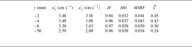
As the surface is approached, the vertical component of the normal Reynolds stresses is redirected in the surface-parallel direction (Hunt & Graham Reference Hunt and Graham1978), as signalled by the increasing fluctuations measured along PIV planes (table 2). The measured instantaneous velocity is Reynolds decomposed into the local mean velocity
 $U_i$
and the local velocity fluctuations
 $u_i$
, the former being negligibly small (Li et al. Reference Li, Wang, Qi and Coletti2024; Ruth & Coletti Reference Ruth and Coletti2024). The root mean square of the velocity fluctuations (r.m.s. velocity) is defined as
 $u_i' = \sqrt {\overline {u_i^2}}$
. To evaluate to which degree the surface flow approximates homogeneous and isotropic conditions, we follow Carter et al. (Reference Carter, Petersen, Amili and Coletti2016) and compute the small-scale isotropic factor
 $\textit{IF} = \overline {|(\partial u_x/\partial x)/(\partial u_y/\partial y)|}$
, the homogeneity deviation
 $\textit{HD} = 2\sigma _{u}/u'$
(where
 $\sigma _{u}$
is the spatial standard deviation of the local ensemble average of the velocity fluctuations
 $\sqrt {\overline {u_i^2}}$
), and the mean strain-rate factor
 $\textit{MSRF} = \left \langle\sqrt{(\partial U_x / \partial x)^2 + (\partial U_y/\partial y)^2}\right \rangle / \overline{\sqrt{\left \langle(\partial u_x /\partial x)^2+ (\partial u_y/\partial y)^2\right \rangle}}$
. Here,
 $\langle {\cdot }\rangle$
denotes spatial averaging. The values of
 $\textit{IF}$
,
 $\textit{HD}$
and
 $\textit{MSRF}$
indicate approximate small-scale isotropy, high spatial homogeneity and negligible mean velocity gradients along the
 $x{-}y$
plane.
Main sub-surface turbulence statistics for the case
 $\textit{Re}_{\lambda }=326$
. Here,
 $z$
is the distance between the turbulence free surface and the PIV measurement plane, and
 $u_x'$
and
 $u_y'$
are the r.m.s. velocities parallel and perpendicular to the jetting direction, respectively. The compressibility coefficient
 $\overline {\mathcal{C}}$
, the small-scale isotropy factor IF, the homogeneity deviation HD and the mean strain-rate factor MSRF are defined in the text.

To describe the topology of the surface velocity field, we consider the reduced velocity gradient tensor
 $\tilde {\boldsymbol {A}}$
, i.e. the upper
 $2\times 2$
block of the full velocity gradient tensor
 $A_{\textit{ij}}=\partial u_i/\partial x_j$
, defined by in-plane gradients of the surface-parallel velocity components (Cardesa et al. Reference Cardesa, Mistry, Gan and Dawson2013; Qi et al. Reference Qi, Xu and Coletti2025b
). One of the key features of free-surface turbulence is the exchange of mass and energy with the bulk, through upwelling and downwelling structures that carry fluid towards and from the surface, respectively (Pan & Banerjee Reference Pan and Banerjee1995). The kinematic boundary condition implies that the surface divergence
 $\mathcal{D} = \tilde {A}_{\textit{ii}}$
is positive above upwellings and negative above downwellings. These regions of expansion and compression reflect the non-solenoidal nature of free-surface flows, quantified by the compressibility coefficient
 $\overline {\mathcal{C}} = \overline {\tilde {A}_{\textit{ii}}^2}/\overline { \tilde {A}_{\textit{ij}}^2}$
(Eckhardt & Schumacher Reference Eckhardt and Schumacher2001; Goldburg et al. Reference Goldburg, Cressman, Vörös, Eckhardt and Schumacher2001; Cressman et al. Reference Cressman, Davoudi, Goldburg and Schumacher2004). The level of compressibility has far-reaching consequences for the relative motion (Csanady Reference Csanady1963; Li et al. Reference Li, Wang, Qi and Coletti2024) and spatial distribution of floating particles (Boffetta et al. Reference Boffetta, Davoudi, Eckhardt and Schumacher2004; Lovecchio, Marchioli & Soldati Reference Lovecchio, Marchioli and Soldati2013; Li et al. Reference Li, Sanness Salmon, Hassaini, Chang, Mucignat and Coletti2025). As we will show, it is crucial for the inter-scale energy transfer, too. Approaching the surface, the compressibility coefficient (which in the bulk is comparable to the theoretical value
 $\overline {\mathcal{C}} = 1/6$
expected for a 2-D cut through 3-D HIT; Boffetta et al. Reference Boffetta, Davoudi, Eckhardt and Schumacher2004) approaches the condition
 $\overline {\mathcal{C}}=0.5$
, implying that the in-plane longitudinal velocity gradients are uncorrelated,
 $\overline {(\partial u_x/\partial x)(\partial u_y/\partial y)}\approx 0$
(Eckhardt & Schumacher Reference Eckhardt and Schumacher2001; Goldburg et al. Reference Goldburg, Cressman, Vörös, Eckhardt and Schumacher2001; Cressman et al. Reference Cressman, Davoudi, Goldburg and Schumacher2004; Li et al. Reference Li, Sanness Salmon, Hassaini, Chang, Mucignat and Coletti2025).
3. Results
3.1. Compressibility of surface flow
To characterise the flow topology of the compressible surface flow, we consider the joint probability distribution function (p.d.f.) of the two invariants of the reduced velocity gradient tensor
 $\tilde {A}$
,
 $p = -\tilde {A}_{\textit{ii}}$
and
 $q = -\det(\tilde {A})$
, respectively (Perry & Chong Reference Perry and Chong1994). The former characterises the divergence of the surface flow, while the latter captures the combined instantaneous stretching and rotation rates along the two principal directions. As shown in figures 2(a1–a4), the joint p.d.f.s exhibit a characteristic teapot shape typical of 2-D sections across 3-D turbulent flows (Cardesa et al. Reference Cardesa, Mistry, Gan and Dawson2013; Carter & Coletti Reference Carter and Coletti2018). Notably, the probability distribution of
 $p$
displays heavier tails as the free surface is approached, indicating increased probability of intense expanding and contracting pattern (Qi et al. Reference Qi, Xu and Coletti2025b
), consistent with the observation that
 $\overline {\mathcal{C}}$
grows approaching the surface. The red dashed line in each image marks
 $q=p^2/4$
, i.e. the boundary across which the local flow topology changes between stable/unstable foci and stable/unstable nodes. This indicates the transition between focus-type (rotation-dominated) and node-type (strain-dominated) regions in the phase portrait (Perry & Chong Reference Perry and Chong1994). Note that the
 $p{-}q$
joint p.d.f. of the 2-D surface velocity field shows a pattern differing significantly from the one measured in 2-D sections of 3-D turbulence in the bulk of the water tank. The latter is reported in figure 7 in Appendix A, and matches the pattern expected in homogeneous regions of 3-D turbulence (Cardesa et al. Reference Cardesa, Mistry, Gan and Dawson2013).
(a) The joint p.d.f.s of normalised
 $p$
and
 $q$
at
 $\textit{Re}_\lambda = 326$
along the 2-D PIV plane for all the considered cases at different distances from the free surface: (a1) 50 mm, (a2) 6 mm, (a3) 4 mm, (a4) 2 mm. The logarithmic contours range from
 $10^{-2}$
to
 $10^{1}$
, with adjacent contours being separated by half a decade. In all four panels, the red dashed lines mark
 $q = p^2/4$
. (b) The p.d.f.s of instantaneous spatially averaged compressibility coefficient
 $\langle \mathcal{C}\rangle = \langle \tilde {A}_{\textit{ii}}^2\rangle /\langle \tilde {A}_{\textit{ij}}^2\rangle$
. (c) Instantaneous divergence and velocity field on the free surface with instantaneous compressibility coefficients (c1)
 $\langle \mathcal{C}\rangle = 0.24$
and (c2)
 $\langle \mathcal{C}\rangle = 0.67$
. The colour map represents the local divergence
 $\mathcal{D}$
normalised by the Kolmogorov time scale
 $\tau _\eta$
, and the arrows indicate the velocity vector
 $\boldsymbol {u}$
.

Figure 2(b) plots the p.d.f.s of instantaneous spatially averaged compressibility coefficient
 $\langle \mathcal{C}\rangle = \langle \tilde {A}_{\textit{ii}}^2\rangle /\langle \tilde {A}_{\textit{ij}}^2\rangle$
. It is shown that the peak of the p.d.f. moves towards higher value of
 $\left \langle \mathcal{C}\right \rangle$
, and the distribution also becomes more spread out. Near the surface, figures 2(c1,c2) illustrate two instantaneous fields of normalised near-surface divergence
 $\mathcal{D}\tau _\eta$
(where
 $\tau _\eta$
is the Kolmogorov time scale) associated with different instantaneous values of
 $\left \langle \mathcal{C}\right \rangle$
. When the latter is large, strongly divergent and convergent flow regions are visible.
3.2. Inter-scale energy transfer and flow structure
Focusing on this near-surface plane, we then analyse the inter-scale energy transfer conditioned on the spatially averaged divergence
 $\langle \mathcal{D} \rangle$
. The probability distribution of
 $\langle \mathcal{D}\rangle \tau _\eta$
is nearly a Gaussian with nearly zero mean and standard deviation
 $\sigma _{\langle \mathcal{D}\rangle } \approx 0.027$
. Via the nominal threshold
 $\pm 1.5\sigma _{\langle \mathcal{D}\rangle } \approx \pm 0.04$
, we define four flow states based on the magnitude and sign of the divergence:
 $\langle \mathcal{D}\rangle \tau _\eta \lt -0.04$
,
 $\langle \mathcal{D}\rangle \tau _\eta \in [-0.04,0]$
,
 $\langle \mathcal{D}\rangle \tau _\eta \in [0,0.04]$
and
 $\langle \mathcal{D}\rangle \tau _\eta \gt 0.04$
. (Somewhat different values of the threshold do not alter the outcome of the following analysis.) With this definition, the probability of the occurrence of strong-divergence states
 $(|\langle \mathcal{D}\rangle |\,\tau _\eta \gt 0.04)$
is approximately 13 %. As the flow is approximately homogeneous and isotropic along the measurement plane, we use polar coordinates and focus on the radial component of the nonlinear inter-scale energy transfer rate
 $\varPi _r$
and the energy flux density
 $S_r$
, which are responsible for the transport across scales as discussed in § 1. Figures 3(a1) and 3(b1) display scale-dependent plots of
 $S_r$
and
 $\varPi _r$
, respectively, conditioned on the four above-mentioned states. The existence of a direct energy cascade requires both
 $S_r$
and
 $\varPi _r$
to be negative, whereas the two should be positive for the cascade to be inverse (Portela et al. Reference Portela, Papadakis and Vassilicos2017). In the present case, when the divergence is strongly positive (
 $\langle \mathcal{D}\rangle \tau _\eta \gt 0.04$
), an intense inverse energy cascade is realised, and vice versa when it is strongly negative: as
 $\langle \mathcal{D}\rangle$
shifts from negative to positive, the direction of the inter-scale energy transfer changes. The magnitudes of
 $S_r$
and
 $\varPi _r$
in weak-divergence states (
 $|\langle \mathcal{D}\rangle |\,\tau _\eta \lt 0.04$
) are significantly smaller than those in strong-divergence states, although the latter occur much less frequently. This indicates that intense and relatively rare compressive/expansive motions are the main drivers of the energy cascade at the free surface. Remarkably, normalisation by the turbulent dissipation in the bulk,
 $\epsilon _{\textit{bulk}}$
, reveals that the inter-scale fluxes in strong-divergence states are much higher than away from the surface, where on average
 $\varPi _r\approx \epsilon _{\textit{bulk}}$
. The polar diagrams in figures 3(a2) and 3(b2) confirm that despite the large-scale anisotropy due to the directional forcing, the process is approximately isotropic, the radial fluxes being approximately independent on the direction of separation along the surface.
Energy flux density and the nonlinear energy transfer rate measured in the 2-D plane 2 mm away from the free surface. (a1,a2) Radial component of the flux of
 $S_r$
normalised by
 $u^3_\eta$
for four ranges of spatial-averaged divergence. (b1,b2) Radial component of the nonlinear scale-to-scale energy transfer
 $\varPi _r$
normalised by the dissipation rate in the bulk
 $\epsilon _{\textit{bulk}}$
.

While the above analysis is purely statistical, one may expect a correlation between inter-scale energy transfers and local flow structures. To verify this picture, we define highly expansive/compressive structures as contiguous regions satisfying the condition
 $|\mathcal{D}|\gt \alpha _{\mathcal{D}}\sqrt {\overline { \mathcal{D}^2}}$
, where
 $\alpha _{\mathcal{D}}$
is a positive constant. To determine the appropriate value of the constant, we analyse the percolation behaviour of such high-intensity regions. Borrowing approaches employed to identify turbulent coherent structures (Moisy & Jiménez Reference Moisy and Jiménez2004; Carter & Coletti Reference Carter and Coletti2018), we consider how the number and size of the structures changes as the threshold is varied. Figures 4(a1–a4) display a normalised instantaneous divergence
 $\mathcal{D}$
field with the resulting expansive/compressive structures identified by a range of threshold levels. Figure 4(b) indicates that both the number and size of the structures are maximised for
 $\alpha _{\mathcal{D}}\approx 0.8$
. Based on the latter, highly expansive/compressive regions are defined. The broad range of sizes can be appreciated, which results in a power-law size distribution (Qi et al. Reference Qi, Li and Coletti2025a
). The p.d.f.s of the fractional area occupied by highly expansive (
 $A_{\textit{exp}}$
) and highly compressive (
 $A_{\textit{comp}}$
) structures in the field of view (FOV) (of area
 $A_{\textit{FOV}}$
) are similar (figure 4
c), implying that both types of events occur with comparable frequency.
(a1) Normalised instantaneous divergence
 $\mathcal{D}$
field for the measurement in the 2-D plane 2 mm away from the free surface, with resulting expansive/compressive structures identified by thresholds (a2)
 $\alpha _{\mathcal{D}}=0.4$
, (a3)
 $\alpha _{\mathcal{D}}=0.8$
and (a4)
 $\alpha _{\mathcal{D}}=1.2$
. (b) Percolation diagram with the total number (purple) and the mean area (green) of high-intensity structures found in the FOV as a function of thresholds
 $|\mathcal{D}|\gt \alpha _{\mathcal{D}}\sqrt {\overline { \mathcal{D}^2}}$
. (c) The p.d.f. of the portion of area in the FOV for compressive (blue) and expansive (red) structures.

We partition the ensemble of near-surface flow fields in strong-divergence state (
 $(A_{\textit{exp}}+A_{\textit{comp}})/A_{\textit{FOV}}\gt 1/2$
) based on the sign of
 $A_{\textit{exp}}-A_{\textit{comp}}$
. The conditional behaviour of
 $S_r$
and
 $\varPi _r$
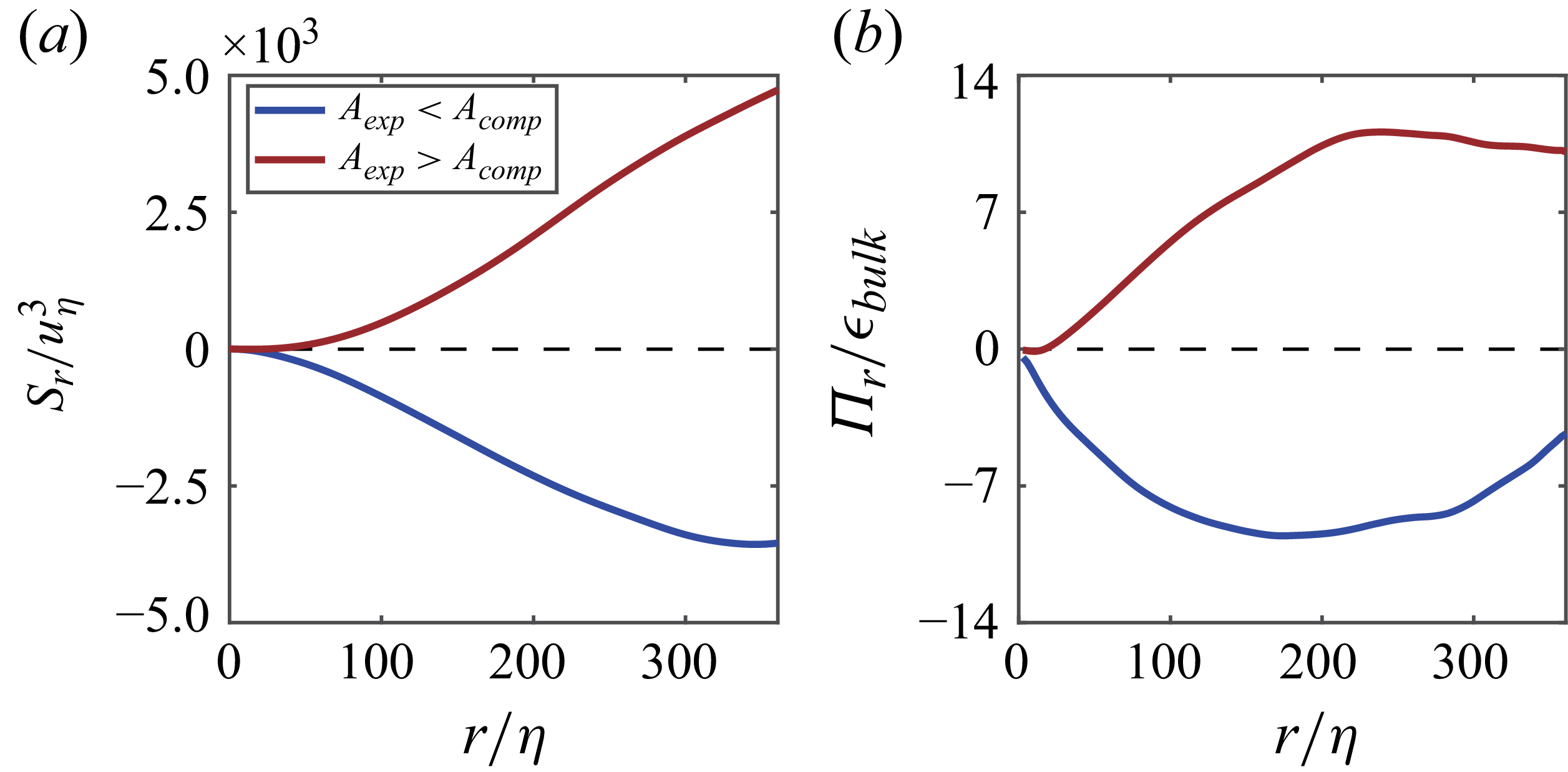
confirms that realisations in which compression (hence downwellings) prevail are characterised by a direct energy cascade from large to small scales, and vice versa; see figure 5. In both situations, the magnitude of
 $\varPi _r$
in the inertial subrange is much greater than in the bulk. This demonstrates that upwellings/expansions and downwellings/compressions are highly effective at transferring energy to larger and smaller scales, respectively. In the framework of the KHMH equation, those structures balance the surface-normal energy fluxes (associated with transport in physical space) with surface-parallel fluxes (in scale space). Because both upwellings and downwellings are characterised by similar intensity and frequency of occurrence, the net inter-scale transfer within the surface flow is marginal. We note that while continuity imposes that the global mass transfers to and from the surface cancel out, some systematic asymmetry in the kinematics of upwellings and downwellings was reported (Guo & Shen Reference Guo and Shen2010; Ruth & Coletti Reference Ruth and Coletti2024), leaving the possibility of a non-zero (albeit weak) net cascade.
Energy flux density and the nonlinear energy transfer rate measured in the 2-D plane 2 mm away from the free surface. (a) Radial component of the flux density
 $S_r$
normalised by
 $u^3_\eta$
for two states. (b) Radial component of the nonlinear scale-to-scale energy transfer
 $\varPi _r$
normalised by the dissipation rate in the bulk
 $\epsilon _{\textit{bulk}}$
. All the calculations are conditioned by the relation between the total area of source
 $A_{\textit{exp}}$
and sink
 $A_{\textit{comp}}$
.

In order to further link the nonlinear energy flux with the local flow structure, we implement the filter-space technique to compute the scale-to-scale energy transfer flux
 $\varPi ^\varDelta$
in physical space, based on the filter velocity field with kernel width
 $\varDelta$
(see, among others, Pan & Banerjee Reference Pan and Banerjee1995; Xiao et al. Reference Xiao, Wan, Chen and Eyink2009; Lovecchio et al. Reference Lovecchio, Zonta and Soldati2015; Yao et al. Reference Yao, Schnaubelt, Szalay, Zaki and Meneveau2024a
; Zhu, Xie & Xia Reference Zhu, Xie and Xia2024). The energy flux at scale
 $\varDelta$
is
 $\varPi ^\varDelta = \tau _{\textit{ij}}^\varDelta s_{\textit{ij}}^\varDelta$
, where
 $\tau _{\textit{ij}}^\varDelta = (u_i u_j)^\varDelta -u_i^\varDelta u_j^\varDelta$
and
 $s_{\textit{ij}}^\varDelta = (\partial _{x_j}u_i^\varDelta +\partial _{x_i}u_j^\varDelta )/2$
are the stress tensor and rate of strain, respectively. As an illustration, figures 6(a,b) show instantaneous snapshots of divergence field
 $\mathcal{D}$
and energy transfer flux field
 $\varPi ^\varDelta$
, respectively, for
 $\varDelta =30\eta$
. These fields bear strong resemblance, with upscale energy fluxes collocated with regions of positive divergence, and vice versa. This can be quantified by the normalised correlation
 $C_{\mathcal{D},\varPi }$
in terms of their inner product (Savelsberg & van de Walter Reference Savelsberg and van de Walter2008):
 \begin{equation} C_{\mathcal{D},\varPi }(\boldsymbol {r})=\dfrac {\overline {\mathcal{D}(\boldsymbol {x}+\boldsymbol {r},t)\boldsymbol{\cdot }\varPi ^\varDelta (\boldsymbol {x},t)}}{\overline {\mathcal{D}\boldsymbol{\cdot }\mathcal{D}}^{1/2}\,\overline {\varPi ^\Delta \boldsymbol{\cdot }\varPi ^\varDelta }^{1/2}}. \end{equation}
Instantaneous snapshots of (a) the divergence field and (b) the energy-flux field (filtering kernel size
 $\varDelta = 30\eta$
), and (c) the 2-D map of normalised correlation
 $C_{\mathcal{D},\varPi }$
in the 2-D plane 2 mm away from the free surface.

A significant correlation between
 $\mathcal{D}$
and
 $\varPi ^\varDelta$
can be seen in figure 6(c), with a maximum
 $C_{\mathcal{D},\varPi }(0) \approx 0.5$
. Much weaker correlation between these quantities is found in the bulk, as shown in Appendix B. Analogous conclusions are drawn for different filter scales. This indicates that at the free surface, the local inter-scale energy transfer is correlated to the divergent flow structures along the free surface.
We close this section with a note on the applicability of the inter-scale energy transfer analysis to free-surface turbulent flows. While the surface flow energy is exchanged with the bulk turbulence beneath and therefore not conserved, this does not undermine the usefulness of the tools that we have adopted. In fact, this approach has been used extensively to uncover the dynamics of a wide array of flows (or portions of them) that exchange energy with adjacent part of the domain, describing pathways of energy transfer across scales, which is useful to both interpreting and modelling them.
In particular, the motion of the ocean free surface has been extensively investigated to determine whether its energy is passed prevalently to larger or smaller scales. For example, Balwada et al. (Reference Balwada, Xie, Marino and Feraco2022) analysed field data from surface drifters in the Gulf of Mexico and found evidence of a dual cascade, with far-reaching consequences for the modelling of oceanic turbulence. Likewise, Tedesco et al. (Reference Tedesco, Baker, Naveira Garabato, Mazloff, Gille, Caulfield and Mashayek2024) used numerical simulations of the near-surface sub-mesoscale turbulence in the Drake Passage to show that eddies and fronts can cause an inverse cascade that replenishes the kinetic energy of mesoscale eddies. Beside surface flows, the dual nature of the cascade has been highlighted in many archetypical configurations, by restricting the analysis to portions of the domain that naturally exchange energy with the surroundings. For example, in wall-bounded turbulence, an inverse cascade was shown to exist at the buffer layer, transferring energy to larger spanwise scales at constant distance from the wall (Jiménez Reference Jiménez1999; Cimarelli et al. Reference Cimarelli, De Angelis, Jiménez and Casciola2016). In rotating Rayleigh–Bénard convection in the geostrophic regime, the spectral transfer term displays energy fluxes from smaller to larger scales when evaluated in the domain excluding the boundary layers, and such an inverse cascade is associated with the formation of a large barotropic vortex (Kunnen et al. Reference Kunnen, Ostilla-Mónico, van der Poel, Verzicco and Lohse2016). By following a strategy similar to that in the present work, those studies revealed important aspects of the whole system dynamics, focusing on specific parts of the entire domain in which energy is not conserved but significant inter-scale energy transfers occur.
4. Conclusion
We have probed experimentally the cascade of energy associated with the free-surface flow above homogeneous turbulence, with negligible mean velocity, shear and waves. The free-surface boundary condition results in profoundly different dynamics compared to both 3-D and 2-D incompressible turbulence. Because energy and enstrophy are not conserved along the surface, classic arguments for the direction and magnitude of the inter-scale transfers cannot be used. We have therefore investigated the intensity, relative prevalence and mechanism behind the local (in space and time) inter-scale energy fluxes to smaller and larger scales. The direct evaluation of the inter-scale energy fluxes indicates that the direction of the cascade within the surface flow depends on its divergence: expansive and compressive states are responsible for energy passing to larger and smaller scales, respectively. Such fluxes in scale space are associated with upwelling and downwelling motions, respectively, and are much more intense than the characteristic ones in the bulk, where the nonlinear inter-scale transfer is in equilibrium with dissipation. Because the upwelling/expansive and downwelling/compressive states are approximately in balance, on average there is no sizeable net energy cascade in the present configuration.
These findings have far-reaching ramifications in the predictive understanding and modelling of this class of flows. In particular, since approximately half of the instantaneous inter-scale transfers of the surface flow energy are inverse, it is imperative for coarse-graining strategies such as large-eddy simulations to account for its backscatter by the sub-grid scales. We note that while the average net energy transfer is negligibly small, the instantaneous/local fluxes in both directions are much larger than the direct transfer rate in the bulk. Therefore, modelling approaches aiming to resolve the spatio-temporal dynamics need to capture the transfers in both directions. An example of the importance of such mechanisms is offered by the recent numerical study of surface geostrophic turbulence in the upper ocean by Xiong et al. (Reference Xiong, Zhang, Li and Xie2025). While their system is distinct from ours due to the role of rotation and buoyancy fluctuations, it also exhibits strikingly similar dynamics associated to the divergence of the surface flow: the compression of cold cyclones by the large-scale background flow sustains downscale energy transfers, while the expansion of warm filaments drives energy upscale. Importantly, the direction of the energy cascade is related to the relative rates of dispersion forwards and backwards in time, which have implications for estimating contaminant spread and concentration fluctuations (Bragg, Ireland & Collins Reference Bragg, Ireland and Collins2016).
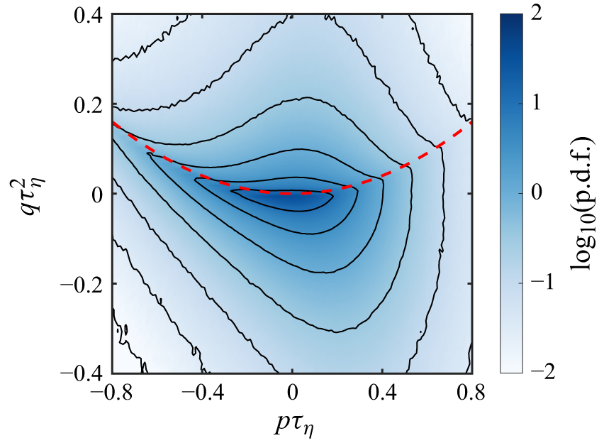
The joint p.d.f. of normalised
 $p$
and
 $q$
at
 $\textit{Re}_\lambda = 326$
along the 2-D PIV plane in the centre of the water tank. The logarithmic contours range from
 $10^{-2}$
to
 $10^{1}$
, with adjacent contours being separated by half a decade, and the red dashed lines mark
 $q = p^2/4$
.

The present work raises numerous further questions. What is the characteristic spatial and temporal extent of the upwelling/expansion and downwelling/compression events? What sets the magnitude of the inter-scale fluxes associated with them? How are these dynamics affected by surface deformation and surfactants? Further studies in these directions are underway.
Acknowledgements
We thank H. Yao and H. Zhu for inspiring discussions and suggestions.
Funding
Y.L. gratefully acknowledges funding from the National Natural Science Foundation of China (NSFC grant no. 12572295), the Opening fund of State Key Laboratory of Nonlinear Mechanics, and the Opening fund of State Key Laboratory for Strength and Vibration of Mechanical Structures (no. SV2023-KF-03). F.C. gratefully acknowledges funding from the Swiss National Science Foundation (project no. 200021-207318).
Declaration of interests
The authors report no conflict of interest.
Appendix A. Joint p.d.f of
 $\boldsymbol{p}$
and
$\boldsymbol{q}$
of the 3-D homogeneous turbulence in the bulk


Figure 7 presents the joint p.d.f. of the normalised quantities
 $p$
and
 $q$
at
 $\textit{Re}_\lambda = 326$
, measured from a 2-D section of the homogeneous turbulence in the bulk flow region. When compared to the results measured 2 mm away from the free surface (as shown in figure 2
a4), the probability distribution of
 $p$
exhibits notably lighter tails, suggesting a significant reduction in the occurrence of intensive expanding and contracting patterns in the bulk of turbulence.
Appendix B. Inter-scale energy transfer of the 3-D homogeneous turbulence in the bulk
Figures 8(a,b) show instantaneous snapshots of the divergence field
 $\mathcal{D}$
and energy transfer flux field
 $\varPi ^\Delta$
with
 $\varDelta =30\eta$
along the 2-D PIV plane in the bulk, respectively. The resemblance between the divergence field and the energy flux field is notably less significant than that along the free surface, which can be also seen in the correlation relation in figure 8(c), i.e. the maximum correlation
 $\mathcal{C}_{\mathcal{D},\varPi }(0) \approx 0.2$
.
Instantaneous snapshots of (a) the divergence field and (b) the energy flux field (filtering kernel size
 $\varDelta = 30\eta$
), and (c) the 2-D map of normalised correlation
 $C_{\mathcal{D},\varPi }$
in the 2-D plane in the bulk far away from the free surface.