



1. Introduction
In recent years, with the growing demand for low-noise and low-drag operational performance in the aerospace, high-speed rail and wind power generation sectors, flow-induced noise problems caused by bluff body structures in high-speed flows have gradually emerged as a critical bottleneck restricting performance improvements (Thompson et al. Reference Thompson, Latorre Iglesias, Liu, Zhu and Hu2015; Mousavi & Kamali Reference Mousavi and Kamali2020; Zhao et al. Reference Zhao, Okolo, Neri, Chen, Kennedy and Bennett2020). The flow around a circular cylinder, a canonical bluff body, exhibits a range of complex unsteady dynamics, including boundary layer transition, flow separation, shear layer instability, vortex shedding and turbulent wake evolution (Strouhal Reference Strouhal1878; Williamson Reference Williamson1996; Norberg Reference Norberg2003; Williamson & Govardhan Reference Williamson and Govardhan2004). These coupled flow mechanisms not only dominate the overall flow field dynamics but also constitute the primary sources of aerodynamic noise. In the subcritical Reynolds number regime, the boundary layer on the cylinder surface undergoes rapid laminar-to-turbulent transition after separation, forming highly spatiotemporally coherent periodic vortex-shedding structures, which give rise to the well-known Kármán vortex street (Zhu et al. Reference Zhu, Dong and Du2025). This process is accompanied by strong periodic pressure fluctuations, resulting in pronounced tonal noise (Maryami & Liu Reference Maryami and Liu2024; Maryami et al. Reference Maryami, Arcondoulis and Liu2024a , Reference Maryami, Guo, Naseer and Liu2024b ). Furthermore, vortex breakdown and its interaction with the turbulent wake induce additional broadband turbulent noise components.
The formation of periodic vortices not only enhances pressure asymmetry around the cylinder – contributing significantly to aerodynamic drag – but also induces periodic lift fluctuations, acting as the dominant mechanism for flow-induced noise generation. Therefore, effective control of vortex shedding is crucial for achieving both noise and drag reduction (Rashidi et al. Reference Rashidi, Hayatdavoodi and Esfahani2016). Among various flow control strategies, passive control methods such as splitter plates (Zhou et al. Reference Zhou, Qiu, Li and Liu2025a ) and helical strakes (Tang et al. Reference Tang, Fan, Wang and Tan2024), as well as active control methods like blowing/suction (Rastan et al. Reference Rastan, Sohankar, Doolan, Moreau, Shirani and Alam2019; Jia & Xu Reference Jia and Xu2025), have been widely studied. In recent years, forced rotation has emerged as a promising active control technique (Choi et al. Reference Choi, Jeon and Kim2008; Tang et al. Reference Tang, Zhu, Song, Ma and Zhou2022; Wang et al. Reference Wang, Zhu, He and Zhang2025). By rotating the cylinder around its central axis, this method actively modulates the boundary layer properties, which in turn influences shear-layer stability and alters the separation location. Such modifications can delay or even suppress periodic vortex shedding, thereby weakening the formation of the Kármán vortex street (Aljure et al. Reference Aljure, Rodríguez, Lehmkuhl, Pérez-Segarra and Oliva2015). Building on these aerodynamic effects, several studies have explored the potential of forced rotation for noise control. For instance, Iida et al. (Reference Iida, Muzuno and Brown2004) numerically demonstrated a direct relationship between wake vortex dynamics and noise reduction under rotation. Similarly, Hu et al. (Reference Hu, Zhang and Wang2018) showed that rotation could significantly reduce acoustic wave radiation perpendicular to the free stream. Extending this work, Souri & Mojra (Reference Souri and Mojra2021) investigated how varying rotation ratios affects noise levels using unsteady Reynolds-averaged Navier–Stokes simulations coupled with the Ffowcs Williams–Hawkings (FW–H) equation. More recently, Yang et al. (Reference Yang, Liu, Chen, Zhang and Bi2025b ) examined the three-dimensional (3-D) flow field under forced rotation, although their study did not provide an in-depth analysis of the underlying noise-generation mechanisms. Furthermore, Bao et al. (Reference Bao, Yang, Zhang and Shao2024) integrated rotating cylinders into leading-edge airfoil designs, demonstrating combined benefits in both aerodynamic performance – through improved lift-to-drag ratio – and far-field noise suppression.
Beyond noise reduction, forced rotation also plays a critical role in enhancing aerodynamic performance. The earliest foundational work by Prandtl (Reference Prandtl1925) experimentally demonstrated that the maximum lift coefficient of a rotating cylinder in homogeneous turbulence could reach
 $4\pi$
, establishing the theoretical basis for subsequent studies. Foundational experiments by Tokumaru & Dimotakis (Reference Tokumaru and Dimotakis1991, Reference Tokumaru and Dimotakis1993) demonstrated the efficacy of rotary oscillation in controlling wake structures and modifying lift forces. Schulmeister et al. (Reference Schulmeister, Dahl, Weymouth and Triantafyllou2017) further elucidated the flow control mechanisms, highlighting the potential for drag reduction and wake stabilisation. Extensive research has since mapped the complex flow regimes associated with rotation. For instance, Chen & Rheem (Reference Chen and Rheem2018) provided detailed experimental insights into the flow field evolution, while numerical studies by Mittal & Kumar (Reference Mittal and Kumar2003) and Kumar et al. (Reference Kumar, Cantu and Gonzalez2011) systematically identified wake transitions and instabilities across various rotation rates. A comprehensive review of these rotation-induced wake transitions was later provided by Rao et al. (Reference Rao, Radi, Leontini, Thompson, Sheridan and Hourigan2015). Building on this, numerous investigations have explored the aerodynamic effects of rotation across a wide range of configurations and Reynolds numbers (defined as
 $Re = U_{\infty }D/\nu$
, where
 $U_{\infty }$
is the free stream velocity,
 $D$
is the cylinder diameter and
 $\nu$
is the kinematic viscosity). At moderate Reynolds numbers, Aljure et al. (Reference Aljure, Rodríguez, Lehmkuhl, Pérez-Segarra and Oliva2015) conducted direct numerical simulations (DNS) at
 $Re = 5 \times 10^3$
with rotation ratios ranging from 0 to 5, showing that increasing rotation deflects the wake, suppresses turbulence, enhances lift and reduces drag, with an optimal ratio that minimises lift fluctuations. Using the same approach, Massaro et al. (Reference Massaro, Karp, Jansson, Markidis and Schlatter2024) extended these findings to
 $Re = 3\times 10^4$
, confirming that higher rotation ratios effectively suppress vortex shedding. Complementing these numerical studies, Ezadi Yazdi et al. (Reference Ezadi Yazdi, Rad and Khoshnevis2019) performed experiments and demonstrated that rotation delays flow separation and reduces drag over a range of Reynolds numbers from
 $5.9\times 10^3$
to
 $1.18\times 10^4$
. At higher Reynolds numbers, Karabelas et al. (Reference Karabelas, Argyropoulos and Markatos2012) performed two-dimensional (2-D) simulations for
 $Re$
ranging from
 $5\times 10^5$
to
 $5\times 10^6$
, demonstrating that increasing rotation progressively stabilises the wake by suppressing vortex shedding. Complementing this, Cao et al. (Reference Cao, Lin, Sun, Li and Jiao2025) reported that a rotation ratio of 2.5 achieved the optimal lift-to-drag ratio at
 $Re = 8.215\times 10^5$
, offering valuable insights for marine propulsion system design. Beyond single-cylinder studies, multicylinder configurations have also been examined, with a focus on the effects of spacing and relative rotation speed on wake dynamics and aerodynamic forces (Ali et al. Reference Ali, Munir and Zhao2023; Siddiqui et al. Reference Siddiqui, Munir, Ali, Zhao, Duan and Qadri2024). Recently, Wang et al. (Reference Wang, Zhu, He and Zhang2025) introduced a hybrid flapping-wing concept that combines leading-edge rotation with trailing-edge oscillation, significantly improving lift and energy conversion efficiency and opening new possibilities for bioinspired aerial vehicle design.
Despite substantial research on the wake dynamics and aerodynamic responses, investigations into the aeroacoustic characteristics of rotating cylinders are relatively sparse but gradually increasing. Notably, Ganta et al. (Reference Ganta, Mahato and Bhumkar2019) analysed the modulation of sound waves for a rotary oscillating cylinder at a low Reynolds number of
 $Re=150$
, and subsequently extended their work to predict aerodynamic sound generated by combined steady rotation and oscillation at the same Reynolds number (Ganta et al. Reference Ganta, Mahato and Bhumkar2020). These studies laid the important groundwork for understanding noise generation with dynamic boundaries. However, distinct from these oscillatory or hybrid configurations, the aeroacoustic mechanisms of steady high-speed rotation at high Reynolds numbers (e.g. in the subcritical flow regime) remain underexplored. It is widely acknowledged that the aerodynamic noise of stationary cylinders primarily originates from periodic wall pressure fluctuations induced by alternating vortex shedding (Maryami & Liu Reference Maryami and Liu2024). As vortices shed alternately from either side of the cylinder, they generate antiphase pressure pulses on the upper and lower surfaces, forming the main sound source. Thomas & Bull (Reference Thomas and Bull1983) emphasised that turbulent velocity fluctuations in the wake are a major contributor to wall pressure disturbances, which in turn drive noise generation. Maryami et al. (Reference Maryami, Arcondoulis and Liu2024a
) and Pan & Ye (Reference Pan and Ye2025) applied coherence analysis to investigate the correlation between velocity fluctuations and surface pressure signals. In our previous studies, Yang et al. (Reference Yang, Bao, Liu, Song, Maryami and Bi2025a
) established the fundamental aerodynamic and aeroacoustic responses of a forced rotating cylinder at a subcritical Reynolds number and demonstrated the feasibility of rotation-based noise control. More recently, Yang et al. (Reference Yang, Maryami, Liu, Bao, Song and Bi2026) conducted a broad parametric investigation over
 $ 0\leqslant \alpha \leqslant 5$
, identifying the global aerodynamic and aeroacoustic regimes and examining the associated changes in mean separation, wall-pressure spectra, spanwise pressure coherence, instantaneous 3-D vortex structures and energy-ranked proper orthogonal decomposition modes.
From an engineering perspective, forced rotation could potentially be implemented using a lightweight rotating sleeve mounted around a bluff structural member, rather than by rotating the entire load-bearing component. Potential applications include the control of aerodynamic noise from the main struts and braces of aircraft landing gear and from the cylindrical or bluff supporting members of high-speed-train pantographs. By modifying the near-wall momentum, separation behaviour and wake coherence, such a sleeve may reduce both the aerodynamic self-noise of an individual member and the unsteady wake impinging on downstream components. This concept remains exploratory, and its practical implementation requires further assessment of finite-span effects, component interactions, actuation power and mechanical integration.
Nevertheless, several aspects of the underlying spatiotemporal organisation remain unresolved. First, the 3-D spatial organisation associated with the split spectral components at low rotation has not been identified, and it remains unclear whether the reduced acoustic radiation results solely from weaker fluctuations or also from a loss of spanwise phase synchronisation. Second, the spatial relationship between unsteady wall-pressure loading and volumetric wake disturbances has not been characterised over the representative rotation regimes. Third, the frequency-specific transition of the dominant 3-D wake topology, particularly from the natural shedding mode to the low-frequency structures observed at high rotation, requires further clarification.
The present study therefore builds on the preceding parametric investigations by selecting five representative conditions,
 $ \alpha$
= 0, 0.5, 1, 2 and 4, and focusing on their frequency-resolved near-field and 3-D wake dynamics. The analysis combines surface-pressure and wake statistics with selected spatiotemporal and modal diagnostics to examine the evolution of source coherence, wall–wake coupling and dominant coherent structures. The objective is not to repeat the global dependence on rotation ratio, but to determine how the representative acoustic signatures are connected to the corresponding 3-D flow organisation. Wind-tunnel measurements are additionally used to assess the far-field acoustic predictions.
The remainder of this paper is organised as follows: § 2 describes the numerical and experimental methods, while § 3 examines the global acoustic response, near-field loading, wake dynamics and 3-D flow organisation. The principal findings, limitations and implications are summarised in § 4.
2. Methodology
2.1. Flow and acoustic methods
Both the flow field and acoustic field simulations in this study were performed using the open-source finite volume computational platform OpenFOAM. Owing to its highly modular and open framework, OpenFOAM has been widely used for the numerical simulation of multiphysics processes such as complex turbulence, heat transfer, combustion and aeroacoustics, providing a flexible and powerful solution environment for coupled multiphysics problems (Weller et al. Reference Weller, Tabor, Jasak and Fureby1998).
For the flow field simulations, large-eddy simulation (LES) is employed, with the wall-adapting local eddy-viscosity model used to represent the effects of the unresolved turbulent scales. The transient incompressible solver pimpleFoam, based on the PIMPLE pressure–velocity coupling algorithm, is used. The PIMPLE algorithm combines features of the pressure-implicit split-operator and semi-implicit method for pressure-linked equations algorithms, providing robust and computationally efficient pressure–velocity coupling. For spatial discretisation, the gradient terms are evaluated using the Gauss linear scheme, while the Laplacian terms are discretised using the Gauss linear corrected scheme to account for mesh non-orthogonality. The convective term in the momentum equation is treated using the linear-upwind stabilised transport (LUST) scheme, Gauss LUST grad(U), which blends central and upwind-biased discretisations to provide a balance between spatial accuracy and numerical robustness. Linear interpolation is used for face-centred quantities, and corrected surface-normal gradients are employed. Time integration is performed using the second-order implicit backward-differencing scheme.
For acoustic field calculations, the FW–H equation is employed to model and predict the far-field aerodynamic noise generated by the unsteady flow field (Ffowcs Williams & Hawkings Reference Williams, John and Hawkings1969). The FW–H equation is derived from Lighthill’s classical acoustic analogy (Lighthill Reference Lighthill1952, Reference Lighthill1954) and relates unsteady flow-induced mass and momentum fluctuations to the radiated acoustic pressure through volume and surface source terms. It is one of the most widely used approaches for far-field noise prediction in engineering aeroacoustics. Under the present low-Mach-number condition (
 $Ma=0.08$
), the volumetric quadrupole contribution is expected to be small relative to the surface-loading contribution and is therefore neglected. In addition, because the cylinder undergoes purely tangential rotation, the normal velocity of the impermeable cylinder surface is zero. Consequently, the thickness contribution associated with normal surface motion vanishes. The far-field sound is therefore evaluated by retaining the loading dipole term associated with the unsteady aerodynamic forces on the cylinder surface. The cylinder wall is used as the FW–H integration surface, allowing the unsteady surface loading induced by the rotating flow to be directly incorporated into the acoustic prediction. This acoustic modelling strategy has been successfully applied and validated in a range of low-speed external-flow aeroacoustic problems, including configurations involving bluff bodies and actively controlled surfaces (Yang et al. Reference Yang, Feng, Peng, Tong and Bao2022, Reference Yang, Arcondoulis, Yang, Guo, Maryami, Bi and Liu2023, Reference Yang, Liu, Zhang and Bi2024, Reference Yang, Liu, Chen, Zhang and Bi2025b
). Its applicability to the present rotating-cylinder configuration is further assessed through the wind-tunnel comparison presented in Appendix B.
2.2. Physical model, mesh topology and boundary conditions
The Reynolds number in this study is set to
 $Re = 4.7 \times 10^4$
, based on a cylinder diameter of
 $D = 0.025$
m and a free stream velocity of
 $U_\infty = 27.2$
m s−1. The corresponding Mach number is
 $Ma = 0.08$
, indicating a typical low-Mach-number incompressible flow regime. The overall structure of the 3-D computational domain, the boundary condition set-up and the mesh generation strategy are illustrated in figure 1. As shown in figure 1(a), the domain inlet is located on the left-hand side (marked in red), where a uniform and steady velocity boundary condition is applied:
 $u = U_\infty$
,
 $v = 0$
, with
 $u$
and
 $v$
denoting the velocity components in the
 $x$
and
 $y$
directions, respectively. The outlet is located on the right-hand side (marked in blue), where Neumann-type boundary conditions
 $\partial u/\partial x = 0$
and
 $\partial v/\partial x = 0$
are imposed to allow smooth fluid outflow. The spanwise (
 $z$
-direction) boundaries are set as periodic to simulate an infinitely long cylinder and eliminate end effects. On the cylinder surface, a no-slip boundary condition is applied for the stationary case, enforcing zero wall velocity. For rotating cases, the tangential wall velocity is prescribed based on the angular velocity
 $\omega _r$
, consistent with the direction of rotation. The non-dimensional rotation ratio is defined as
 $\alpha = {\omega _r D}/{2 U_\infty }$
. Five rotation cases are investigated in this study:
 $\alpha = 0$
, 0.5, 1, 2 and 4. The case
 $\alpha = 0$
corresponds to the stationary cylinder, which serves as the baseline for subsequent comparisons. The coordinate system is defined with the geometric centre of the cylinder as the origin. The
 $x$
-axis is aligned with the free stream direction, the
 $y$
-axis is oriented transversely and the
 $z$
-axis is spanwise. The windward side of the cylinder is defined as
 $\theta = 0^\circ$
, the leeward side as
 $\theta = 180^\circ$
, and the azimuthal angle
 $\theta$
increases in the clockwise direction.
The circular computational domain has a diameter of
 $40D$
, and the spanwise length is
 $L_z = 4D$
, sufficient to capture vortex shedding, wake development and associated 3-D disturbance structures (Zhdanov et al. Reference Zhdanov, Green and Busse2023). Recent studies have underscored the necessity of 3-D simulations for aeroacoustic predictions, demonstrating that 2-D models can significantly overestimate noise levels by neglecting spanwise decorrelation effects (Leung & Redonnet Reference Leung and Redonnet2024). Figure 1(b) presents the overall layout of the 3-D structured mesh and a magnified view of the near-wall region. An O-type structured hexahedral mesh is employed throughout the domain to enhance boundary layer resolution and improve numerical accuracy. The height of the first cell adjacent to the wall is set to
 $0.0002D$
, with a radial expansion ratio of
 $1.02$
, and the total number of grid cells is approximately
 $6\times10^6$
. The non-dimensional wall-normal mesh parameter is controlled at
 $y^+ \lt 0.3$
, while the streamwise and spanwise grid spacings satisfy
 $\Delta x^+ \lt 18$
and
 $\Delta z^+ \lt 60$
, respectively, meeting the basic resolution requirements for LES near-wall modelling (Wagner et al. Reference Wagner, Hüttl and Sagaut2007). To ensure numerical stability in time integration, the time step is selected to satisfy the Courant–Friedrichs–Lewy condition with a value less than 1. While the stationary cylinder case was validated in our previous work (Yang et al. Reference Yang, Liu, Chen, Zhang and Bi2025b
), details regarding grid independence and validation for rotating conditions are provided in the appendices.
(
 $ a$
) Schematic of the computational domain and boundary condition settings. (
 $ b$
) Illustration of the mesh configuration for flow around the cylinder, including the overall grid layout and local refinement near the cylinder wall.

In the central
 $x$
–
 $y$
plane, a circular far-field microphone array is arranged on the midspan section of the cylinder to capture aerodynamic noise signals. The array consists of 24 microphones evenly distributed along a circle with a radius of
 $80D$
, centred at the geometric centre of the cylinder, ensuring omnidirectional coverage of the far-field acoustic pressure field. The observed acoustic pressure signals are analysed using Welch’s method (Welch Reference Welch1967) to obtain the power spectral density (PSD) of the far-field noise, denoted as
 $\varPhi _{pp}$
(in dB Hz
 $^{-1}$
). The PSD is computed using the following expression:
 \begin{equation} \varPhi _{pp} = 10 \log _{10} \left ( \frac {\phi _{pp}}{p_0^2} \right ), \end{equation}
where
 $\phi _{pp}$
represents the raw PSD of the pressure signal at the microphone location (in Pa
 $^2$
Hz
 $^{-1}$
), and
 $p_0$
is the reference sound pressure, set as
 $2 \times 10^{-5}$
Pa.
Furthermore, to evaluate the overall aerodynamic noise level under different rotation conditions, the overall sound pressure level (OASPL) is obtained by integrating
 $\phi _{pp}$
over the target frequency range. The corresponding non-dimensional Strouhal number is defined as
 $St = \textit{fD}/U_\infty$
, and the integration range is set as
 $0.05 \leqslant St \leqslant 10$
. The OASPL is calculated using the following equation:
 \begin{equation} \textit{OASPL} = 10 \log _{10} \left ( \frac {\int \phi _{pp} \mathrm{d}f}{p_0^2} \right ). \end{equation}
As an integrated measure of the far-field sound-pressure level, OASPL characterises the overall acoustic response over the specified frequency range.
2.3. Continuous wavelet transform
In vortex-shedding-dominated aeroacoustic flows, the aerodynamic and acoustic signals may exhibit non-stationary behaviour, including time-varying frequency components and transient events. The fast Fourier transform provides the global frequency content of a signal but does not retain information about the temporal localisation of individual spectral components. The wavelet transform is therefore employed as a time–frequency analysis tool to examine the temporal evolution of the lift and acoustic responses over different frequency scales (Fujimoto & Rinoshika Reference Fujimoto and Rinoshika2015; Maryami & Ali Reference Maryami and Ali2023; Yang et al. Reference Yang, Liu, Zhang and Bi2024).
The continuous wavelet transform (CWT) (Mallat Reference Mallat1999) is applied to the lift-coefficient and far-field acoustic-pressure signals. The CWT is defined as
 \begin{equation} W_x(a,\tau ) = \frac {1}{a} \int _{-\infty }^{+\infty } x(t) \psi ^* \left ( \frac {t-\tau }{a} \right ) \,\mathrm{d}t, \qquad a\gt 0, \end{equation}
where
 $x(t)$
is the input signal,
 $W_x(a,\tau )$
is the complex wavelet coefficient at scale
 $a$
and time location
 $\tau$
, and
 $\psi ^*$
denotes the complex conjugate of the analysing wavelet. The analytic Morlet wavelet is employed in the present analysis. Its complex-valued form provides simultaneous amplitude and phase information with good time–frequency localisation, making it suitable for characterising the non-stationary lift and acoustic responses (Morlet et al. Reference Morlet, Arens, Fourgeau and Glard1982). The frequencies associated with the wavelet scales are converted to Strouhal numbers using
 $St = \textit{fD}/U_\infty$
, and the magnitude
 $|W_x(St,t)|$
is used to describe the time-localised spectral content of each signal.
2.4. Dynamic mode decomposition
Unsteady flows are typically characterised by complex multiscale and multifrequency dynamics. Traditional time-domain or frequency-domain analysis methods often struggle to effectively identify the dominant modes and their evolutionary patterns. Therefore, extracting dominant coherent structures and intrinsic dynamical mechanisms from high-dimensional non-stationary flow data is crucial for understanding the evolution of complex flow structures under forced rotation and uncovering potential noise reduction mechanisms.
The tecchnique DMD is a classical data-driven modelling technique that approximates the unsteady flow as the dynamic evolution of a linear system, extracting modal information directly from time-resolved snapshots obtained through experiments or numerical simulations. Compared with proper orthogonal decomposition, DMD not only identifies dominant low-rank structures but also assigns each mode with a distinct characteristic frequency and growth/decay rate (Schmid et al. Reference Schmid, Li, Juniper and Pust2010; Schmid Reference Schmid2010; Taira et al. Reference Taira, Brunton, Dawson, Rowley, Colonius, McKeon, Schmidt, Gordeyev, Theofilis and Ukeiley2017). As such, DMD has been widely applied to mode identification, noise-source localisation and the modal characterisation of unsteady flows. The specific decomposition procedure is described as follows.
-
(i) Snapshot matrix construction
A sequence of 3-D flow field snapshots with time interval
 $\Delta t^*$
is organised into two shifted data matrices,
 \begin{align} \boldsymbol{X}_1 = \begin{bmatrix} \boldsymbol{x}(t_1) & \boldsymbol{x}(t_2) & \boldsymbol{\cdots} & \boldsymbol{x}(t_{m-1})\end{bmatrix} \in \mathbb{R}^{n \times (m-1)}, \\[-28pt] \nonumber \end{align}
 \begin{align} \boldsymbol{X}_2 = \begin{bmatrix} \boldsymbol{x}(t_2) & \boldsymbol{x}(t_3) & \boldsymbol{\cdots} & \boldsymbol{x}(t_m)\end{bmatrix} \in \mathbb{R}^{n \times (m-1)}, \\[0pt] \nonumber \end{align}
where
 $\boldsymbol{x}(t_i) \in \mathbb{R}^n$
is the snapshot vector at time
 $t_i$
. In the present 3-D-DMD analysis, each column vector
 $\boldsymbol{x}(t_i)$
is constructed by reshaping the 3-D velocity field components
 $(u, v, w)$
within the sampling volume into a single high-dimensional vector. Thus,
 $n = 3 \times N_x \times N_y \times N_z$
represents the total degrees of freedom, and
 $m$
is the total number of snapshots. A linear approximation is assumed between adjacent snapshots,
 \begin{equation} \boldsymbol{X}_2 = \boldsymbol{A} \boldsymbol{X}_1, \end{equation}
where
 $\boldsymbol{A} \in \mathbb{R}^{n \times n}$
is the linear evolution operator mapping one state to the next in time.
-
(ii) Singular value decomposition and low-rank projection
To avoid directly computing the high-dimensional operator
 $\boldsymbol{A}$
, singular value decomposition is performed on
 $\boldsymbol{X}_1$
,
 \begin{equation} \boldsymbol{X}_1 = \boldsymbol{U} \varSigma \boldsymbol{V}^T, \end{equation}
where
 $\boldsymbol{U} \in \mathbb{R}^{n \times r}$
,
 $\varSigma \in \mathbb{R}^{r \times r}$
and
 $\boldsymbol{V} \in \mathbb{R}^{(m-1) \times r}$
, with
 $r$
being the truncation rank. The linear operator
 $\boldsymbol{A}$
is then projected into the reduced subspace spanned by
 $\boldsymbol{U}$
,
 \begin{equation} \tilde {\boldsymbol{A}} = \boldsymbol{U}^T \boldsymbol{A} \boldsymbol{U} = \boldsymbol{U}^T \boldsymbol{X}_2 \boldsymbol{V} \varSigma ^{-1}. \end{equation}
An eigendecomposition is performed on the reduced matrix
 $\tilde {\boldsymbol{A}} \in \mathbb{R}^{r \times r}$
,
 \begin{equation} \tilde {\boldsymbol{A}} \boldsymbol{W} = \boldsymbol{W} \boldsymbol{\varLambda }, \end{equation}
where
 $\boldsymbol{\varLambda } = {diag}(\lambda _1, \lambda _2, \boldsymbol{\cdots} , \lambda _r)$
contains the eigenvalues
 $\lambda _{\!j} \in \mathbb{C}$
of the DMD modes, and
 $\boldsymbol{W} \in \mathbb{C}^{r \times r}$
is the matrix of eigenvectors.
-
(iii) Exact mode reconstruction
Following the exact DMD method proposed by Tu (Reference Tu2013), the DMD modes are reconstructed in the original high-dimensional space as
 \begin{equation} \boldsymbol{\varPsi } = \boldsymbol{X}_2 \boldsymbol{V} \varSigma ^{-1} \boldsymbol{W}, \end{equation}
where
 $\boldsymbol{\varPsi }_{\!j} \in \mathbb{C}^n$
denotes the
 $j$
th DMD mode, representing a spatial structure associated with the corresponding eigenvalue. Compared with the traditional formulation
 $\boldsymbol{\varPsi }_{\!j} = \boldsymbol{U} \boldsymbol{w}_{\!j}$
, this approach provides improved physical interpretability for mode-structure reconstruction and relative modal-contribution assessment.
-
(iv) Frequency and growth/decay rate extraction
The temporal evolution of each mode is governed by its eigenvalue
 $\lambda _{\!j}$
, from which the oscillation frequency and growth/decay rate are computed as
 \begin{equation} f_{\!j} = \frac {{Im}(\ln \lambda _{\!j})}{2\pi \Delta t^*}, \quad \sigma _{\!j} = \frac {{Re}(\ln \lambda _{\!j})}{\Delta t^*}, \end{equation}
where
 $f_{\!j}$
is the mode frequency in hertz, and
 $\sigma _{\!j}$
denotes the growth (
 $\sigma _{\!j} \gt 0$
) or decay rate (
 $\sigma _{\!j} \lt 0$
) in
 $\mathrm{s}^{-1}$
. Here, the stability terminology refers to the temporal growth or decay of modes associated with the data-driven DMD evolution operator, rather than to eigenvalues obtained from a linear global-stability analysis of the governing equations.
-
(v) Relative modal-energy indicator
The relative contribution of each mode is evaluated using the squared 2-norm of the corresponding mode vector:
 \begin{equation} P_{\!j}=\|\boldsymbol{\varPsi }_{\!j}\|_2^2 . \end{equation}
Here,
 $P_{\!j}$
is used as a relative modal-energy indicator to compare DMD modes obtained using the same normalisation convention. It is not interpreted as an absolute physical kinetic energy.
-
(vi) Parameter settings
In this study, a total of 2501 snapshots of the instantaneous 3-D velocity field are extracted from the statistically stationary interval
 $t=0.1$
–
 $0.2$
s, after the initial transient has been excluded. The sampling domain covers the near-wake region defined by
 $x/D \in [-2,10]$
,
 $y/D \in [-2,2]$
and
 $z/D \in [-2,2]$
. Each snapshot contains all three velocity components (
 $u$
,
 $v$
and
 $w$
) to capture the spatial evolution of the coherent structures. The temporal interval between consecutive snapshots is
 $\Delta t^*=4\times 10^{-5}$
s, yielding 2500 snapshot intervals and a total sampling duration of
 $0.1$
s. All snapshots are used to construct the DMD model, from which the dominant unsteady coherent structures are extracted and analysed in terms of their characteristic frequencies, modal stability characteristics and relative modal-energy distributions.
3. Results and discussion
3.1. Aeroacoustic characteristics
Figure 2 systematically presents the aeroacoustic characteristics of the flow around the circular cylinder under different rotation ratios (
 $\alpha = 0, 0.5, 1, 2, 4$
), revealing the significant influence of forced rotation on both the generation and radiation mechanisms of aerodynamic noise. Figure 2(a) compares the far-field acoustic spectra. The baseline case is dominated by the vortex-shedding tone at
 $St_0 \approx 0.2$
, together with a higher harmonic near
 $St_2 \approx 0.6$
. At
 $\alpha = 0.5$
, the principal spectral component separates into two peaks,
 $St_{01}\approx 0.18$
and
 $St_{02}\approx 0.23$
, while the tonal level is substantially reduced. A partial recovery of tonal shedding occurs at
 $\alpha =1$
, with the dominant frequency shifting to
 $St\approx 0.24$
. Among the selected conditions, the strongest tonal-noise suppression is obtained at
 $\alpha =2$
. At
 $\alpha =4$
, the classical shedding tone is no longer identifiable and is replaced by a low-frequency broadband ‘hump’ centred approximately at
 $St\approx 0.1$
. These characteristic frequencies are used below to examine the corresponding surface-pressure and wake structures. The one-third-octave-band results in figure 2(b) confirm that the narrowband tonal reduction is accompanied by a broader decrease in the radiated noise, particularly at
 $ \alpha =2$
. Figure 2(c) further shows that rotation modifies both the magnitude and orientation of the predominantly dipolar radiation pattern. Since the detailed dependence of the far-field level and directivity on the rotation ratio has already been reported by Yang et al. (Reference Yang, Maryami, Liu, Bao, Song and Bi2026), the present study uses these results only as the acoustic reference for the subsequent mechanism analysis.
The aeroacoustic characteristics of the flow around the circular cylinder under different rotation ratios (
 $\alpha = 0, 0.5, 1, 2, 4$
): (
 $ a$
) acoustic PSD,
 $\varPhi _{pp}$
, as a function of
 $St$
at the observation point
 $(0, 80D, 0)$
; (
 $ b$
) 1/3-octave-band representation of the acoustic spectra; (
 $ c$
) directivity of the OASPL in the midspan plane (
 $z/D = 0$
). The underlying far-field acoustic signals are from the LES database previously reported by Yang et al. (Reference Yang, Maryami, Liu, Bao, Song and Bi2026).

Time histories of the lift coefficient
 $C_l$
, together with the CWT magnitudes of the lift coefficient,
 $|W_{C_l}|$
, and the corresponding far-field acoustic pressure,
 $|W_{noise}|$
, for different rotation ratios: (a) baseline, (b)
 $\alpha =0.5$
, (c)
 $\alpha =1$
, (d)
 $\alpha =2$
and (e)
 $\alpha =4$
. Subpanels (i)–(iii) show
 $C_l$
,
 $|W_{C_l}|$
and
 $|W_{noise}|$
, respectively.

To examine the effects of rotation on the lift and aeroacoustic responses, figure 3 presents the time history of the lift coefficient
 $C_l$
, together with the CWT magnitudes of the lift coefficient,
 $|W_{C_l}|$
, and the corresponding far-field acoustic pressure,
 $|W_{noise}|$
, for the different rotation ratios. Figure 3(a i–e i) show that the lift response evolves from regular periodic oscillations to increasingly irregular fluctuations as the rotation ratio changes. In the baseline case (figure 3
a i),
 $C_l$
exhibits pronounced periodic variations associated with the classical Kármán vortex street. At
 $\alpha =0.5$
(figure 3
b i), this periodic behaviour is visibly disturbed. Partial periodicity re-emerges at
 $\alpha =1$
(figure 3
c i), although the oscillation remains less regular than in the baseline case. At
 $\alpha =2$
(figure 3
d i), the lift-fluctuation amplitude is substantially reduced. With a further increase to
 $\alpha =4$
(figure 3
e i), the lift signal becomes irregular and contains pronounced low-frequency variations, indicating departure from the classical periodic shedding regime. The corresponding
 $|W_{C_l}|$
distributions are shown in figure 3(a ii–e ii). In the baseline case, the CWT magnitude is concentrated near
 $St\approx 0.2$
, corresponding to the characteristic shedding frequency of the Kármán vortex street. The time–frequency distribution varies non-monotonically with the rotation ratio. At
 $\alpha =0.5$
and
 $2$
(figures 3
b ii and 3
d ii, respectively), the CWT magnitude near
 $St\approx 0.2$
decreases markedly. At
 $\alpha =1$
(figure 3
c ii), a pronounced frequency component remains near
 $St\approx 0.24$
, consistent with the partial recovery of periodic shedding. At
 $\alpha =4$
(figure 3
e ii), the dominant time–frequency content shifts towards a lower-frequency region near
 $St\approx 0.1$
, indicating the emergence of a rotation-induced low-frequency response. The acoustic-pressure CWT magnitudes,
 $|W_{noise}|$
, shown in figure 3(a iii–e iii), exhibit trends that broadly correspond to those of
 $|W_{C_l}|$
. In particular, the suppression, partial recovery and subsequent low-frequency shift of the dominant components occur under the same rotation conditions. This correspondence is consistent with the important role of unsteady lift fluctuations in the predominantly dipolar far-field radiation.
Real parts of the CWT coefficients of the lift coefficient,
 $\Re (W_{C_l})$
, and the corresponding far-field acoustic pressure,
 $\Re (W_{noise})$
, for different rotation ratios: (a) baseline, (b)
 $\alpha =0.5$
, (c)
 $\alpha =1$
, (d)
 $\alpha =2$
and (e)
 $\alpha =4$
.

Figure 4 further illustrates the time–frequency characteristics of the lift coefficient,
 $C_l$
, and the far-field acoustic-pressure signal for the different rotation ratios. The real parts of their CWT coefficients are denoted by
 $\Re (W_{C_l})$
and
 $\Re (W_{noise})$
, respectively. Two recurring features can be identified in the wavelet fields: quasiperiodic banded patterns and time-localised cone-like patterns. The former appear as approximately horizontal sequences of alternating positive and negative coefficients and remain concentrated around a nearly constant Strouhal number. They are therefore consistent with persistent periodic shedding. In contrast, the cone-like patterns extend over a broader frequency range during limited time intervals, indicating transient broadband spectral content rather than a single persistent frequency component. Their coexistence suggests that the dominant periodic response is accompanied by intermittent broadband fluctuations during the deformation and breakdown of the shear layers (Farge Reference Farge1992). The CWT fields thus distinguish persistent narrowband components from time-localised broadband responses, but do not by themselves establish a physical interscale energy-transfer pathway.
In the baseline case, both
 $\Re (W_{C_l})$
and
 $\Re (W_{noise})$
in figure 4(a) exhibit continuous and regularly distributed banded patterns concentrated near
 $St\approx 0.2$
. This behaviour is consistent with organised large-scale Kármán vortex shedding and the corresponding tonal acoustic response. At
 $\alpha =0.5$
(figure 4
b), the amplitude of the banded response decreases, while time-localised broadband features become more evident around the principal frequency range. This change is consistent with weakened periodic organisation and an increased contribution from intermittent fluctuations. At
 $\alpha =1$
(figure 4
c), quasiperiodic banded patterns remain visible, and the dominant frequency shifts slightly upwards to
 $St\approx 0.24$
, consistent with the partial re-establishment of organised shedding. When the rotation ratio increases to
 $\alpha =2$
(figure 4
d), the repetitive patterns become sparse and weak, and the time–frequency response is dominated by low-amplitude, time-localised features. This behaviour indicates strong attenuation of the organised large-scale shedding component and a transition towards a weaker and less regularly organised unsteady-loading response. At
 $\alpha =4$
(figure 4
e), the phase-organised pattern associated with classical vortex shedding is no longer evident. Instead, irregular broadband features appear over a wider range of scales, together with a low-frequency component near
 $St\approx 0.1$
in both the lift and acoustic signals. These features are consistent with intermittent modulation of the near-wall rotating layer rather than a recovery of the classical Kármán mode. The corresponding spatial structures are examined in the subsequent 3-D analyses.
Beyond the qualitative patterns observed in the time–frequency domain, a quantitative comparison is performed to characterise the non-monotonic dependence of the aeroacoustic response on the rotation ratio
 $\alpha$
and to examine the corresponding evolution of the time–frequency content. Figure 5(a) compares the root-mean-square (r.m.s.) lift-coefficient fluctuation,
 $C_{l,{rms}}^{\prime }$
, with the OASPL. The two quantities exhibit closely corresponding non-monotonic trends, consistent with the dominant role of unsteady lift fluctuations in the predominantly dipolar acoustic radiation. Both quantities reach their lowest values among the selected cases at
 $\alpha =2$
, indicating that this condition provides the strongest suppression of unsteady loading and far-field noise. To quantify the CWT distributions and relate them to the macroscopic fluctuation measures, an integrated wavelet measure,
 $E$
, is defined from the squared magnitude of the CWT coefficients over the selected time–frequency region. For the lift and far-field acoustic-pressure signals, the corresponding measures are denoted by
 $E_{C_l}$
and
 $E_{{noise}}$
, respectively. The measure is defined as
 \begin{equation} E = \int _{0.05}^{10} \left [ \frac {1}{T} \int _{t_1}^{t_2} \left |W(St,t)\right |^2 \,\mathrm{d}t \right ] \,\mathrm{d}St, \end{equation}
where
 $W(St,t)$
denotes the CWT coefficient, and
 $T=t_2-t_1=0.1$
s is the duration of the statistically stationary sampling interval. This quantity is used as a comparative integrated measure of the squared CWT magnitude rather than as a strict physical energy. The variations of
 $E_{C_l}$
and
 $E_{{noise}}$
with
 $\alpha$
are shown in figure 5(b). Their variations are consistent with the macroscopic fluctuation trends and provide a quantitative comparison between the time–frequency responses observed in the CWT fields. At
 $\alpha =1$
, both measures exhibit a local increase, corresponding to the partial recovery of the organised periodic components shown in figure 4(c), where the CWT magnitude remains concentrated around the characteristic shedding frequency. At
 $\alpha =2$
, both measures reach their lowest values, consistent with the sparse and weak time–frequency response in figure 4(d) and with the strongest attenuation of unsteady fluctuations among the selected cases. At
 $\alpha =4$
, the integrated measures increase again owing to the enhanced broadband and low-frequency content. This increase is associated with localised near-wall 3-D unsteadiness rather than with a recovery of the classical spanwise-coherent shedding mode.
Quantitative comparison of the non-monotonic variation of the unsteady response with rotation ratio
 $\alpha$
: (a) r.m.s. lift-coefficient fluctuation,
 $C_{l,{rms}}^{\prime }$
, and OASPL; (b) integrated wavelet measures of the lift coefficient,
 $E_{C_l}$
, and far-field acoustic pressure,
 $E_{noise}$
, obtained from the squared CWT magnitude over
 $0.05\lt St\lt 10$
.

3.2. Near-field pressure analysis
To further reveal the modulation mechanism of forced rotation on the surface pressure distribution, figure 6 systematically presents the contours of the time-averaged pressure coefficient (
 $\overline {C}_p$
) and the r.m.s. of the fluctuating pressure coefficient (
 $C_{p,{rms}}^{\prime }$
) along the cylinder span and circumference for different rotation ratios
 $\alpha$
. In the baseline case (
 $\alpha =0$
),
 $\overline {C}_p$
exhibits a typical symmetric distribution. Distinct low-pressure regions form near the separation points of the upper and lower shear layers (
 $\theta \in [60^\circ , 80^\circ ]$
and
 $[280^\circ , 300^\circ ]$
), while a broad constant-pressure zone in the leeward region (
 $[80^\circ , 280^\circ ]$
) marks the recirculation region characteristic of the baseline separated-flow state. When the rotation ratio increases to
 $\alpha = 0.5$
, this symmetry is noticeably disrupted. The low-pressure region on the lower side intensifies significantly (reaching a minimum near
 $\theta \approx 270^\circ$
), whereas the upper-side suction peak weakens. This asymmetry induces a negative lift, indicating the onset of the `lift crisis’ (Cheng et al. Reference Cheng, Pullin and Samtaney2018). Simultaneously, the recirculation region contracts, marking the initial suppression of regular vortex shedding. As
 $\alpha$
increases to 1, the upper low-pressure region expands significantly towards the rear, suggesting enhanced boundary layer attachment due to the Magnus effect. Consequently, the lift coefficient transitions from negative to positive, improving aerodynamic performance. At
 $\alpha =2$
, the asymmetry intensifies: a stable, broad low-pressure region dominates the upper surface, while the lower side transitions to a high-pressure zone. The recirculation region is further compressed and nearly vanishes. Finally, at
 $\alpha = 4$
, the lower side is completely enveloped by high pressure, while the upper side maintains a broad low-pressure state, indicating that the classical alternating shedding pattern is no longer evident.
Contours of (i) time-averaged pressure coefficient (
 $\overline {C}_p$
) and (ii) r.m.s. pressure coefficient fluctuations (
 $C_{p,{rms}}^{\prime }$
) at different rotation ratios
 $\alpha$
: (a) baseline, (b)
 $\alpha = 0.5$
, (c)
 $\alpha = 1$
, (d)
 $\alpha = 2$
, (e)
 $\alpha = 4$
.

The distribution of
 $C_{p,{rms}}^{\prime }$
further elucidates the evolution of unsteady wall pressure fluctuations. For the baseline, peak fluctuation intensities occur near the separation points (
 $\theta \approx 70^\circ$
and
 $290^\circ$
), driven by the oscillating shear layers. A striking phenomenon emerges at
 $\alpha = 0.5$
. While the fluctuation intensity on the upper side diminishes due to stabilisation, the lower side (
 $\theta \approx 270^\circ$
) exhibits a distinct high-intensity band of fluctuations, exceeding even the baseline levels. Although this suggests strong local unsteadiness, it contrasts with the global noise reduction observed in far-field spectra. This implies that while the lower shear layer sheds vigorously near the wall, the resulting structures are highly localised and lack the spanwise coherence necessary for efficient noise radiation. As
 $\alpha$
increases to 2, the upper separation point shifts downstream with low fluctuation levels, and the lower-side fluctuations are effectively suppressed, indicating strong attenuation of the dominant shedding-related wake fluctuations. Finally, at
 $\alpha =4$
, high-intensity pressure fluctuations re-emerge and extend over a broad region of the cylinder surface. These irregular patterns are consistent with the localised near-wall 3-D unsteadiness identified later from the instantaneous vortex and DMD fields. The relatively uniform spanwise distributions of
 $\overline {C}_p$
and
 $C_{p,{rms}}^{\prime }$
indicate approximate spanwise homogeneity of the first- and second-order pressure statistics. This statistical uniformity does not, however, imply spanwise coherence of the instantaneous or frequency-resolved flow structures.
Time–space distribution of the surface pressure coefficient (
 $C_p$
) on the cylinder under different rotation ratios
 $\alpha$
: (a) baseline, (b)
 $\alpha = 0.5$
, (c)
 $\alpha = 1$
, (d)
 $\alpha = 2$
, (e)
 $\alpha = 4$
.

To further explore the impact of forced rotation on the time–space distribution characteristics of the cylinder surface pressure, figure 7 presents the time–space evolution of the surface pressure coefficient
 $C_p$
under different rotation ratios. In the baseline case, the pressure time–space map exhibits a regular periodic stripe structure, corresponding to the vortex shedding frequency of approximately 210 Hz, which is consistent with the frequency spectrum analysis results shown in figure 2(a). It is evident that the pressure fluctuations on the upper and lower surfaces of the cylinder are out of phase, reflecting the alternating shedding of vortices on the top and bottom sides of the cylinder, eventually evolving into the typical Kármán vortex street in the wake. Clear low-pressure fluctuation zones are observed at
 $\theta \approx 70^\circ$
and
 $290^\circ$
, indicating the development of shear layer instability. When the rotation ratio increases to
 $\alpha = 0.5$
, the flow characteristics on the cylinder surface change significantly: the upper-side low-pressure fluctuation zone shifts towards
 $\theta \approx 75^\circ$
, and the vortex shedding process exhibits dual-frequency components, which closely align with the ‘dual-peak’ phenomenon revealed in figure 2(a). Meanwhile, the lower-side low-pressure fluctuation zone around
 $\theta \approx 285^\circ$
shows intense non-stationarity, characterised by the presence of multiple sharp peaks in the pressure signal, indicating enhanced wall pressure fluctuations.
As the rotation ratio further increases to
 $\alpha = 1$
, the upper-side low-pressure zone (
 $\theta \approx 80^\circ$
) regains a stable and clear periodic feature, with a significant expansion of the fluctuation range, indicating the recovery of vortex shedding behaviour. Although the pressure fluctuation near
 $\theta \approx 280^\circ$
on the lower side increases slightly, the sharp peak-like irregular disturbances are significantly reduced, suggesting that the local pressure response becomes more regular. Under the condition of
 $\alpha = 2$
, the upper-side low-pressure zone (
 $\theta \approx 90^\circ$
) tends towards a steady distribution, and the pressure fluctuations further weaken. On the lower side (
 $\theta \approx 270^\circ$
),
 $C_p$
shifts towards higher values, while the periodic pressure pattern progressively weakens, consistent with the suppression of coherent vortex shedding. Finally, under the condition of
 $\alpha = 4$
, the pressure fluctuation regions at
 $\theta \approx 90^\circ$
exhibit partial periodicity, corresponding to flow structures at approximately 125 Hz (
 $ St\approx 0.1$
), which is consistent with the conclusions drawn from figures 2 to 4.
Spanwise distributions of the pressure power spectral density (
 $\varPhi _{pp,s}$
) as a function of
 $St$
at different rotation ratios for three typical circumferential angles,
 $\theta =90^\circ$
,
 $180^\circ$
, and
 $270^\circ$
. Panels (a)–(e) correspond to the baseline case and rotation ratios
 $\alpha =0.5$
,
 $1$
,
 $2$
and
 $4$
, respectively. Subpanels (i) to (iii) correspond to (i)
 $\theta =90^\circ$
(upper side), (ii)
 $\theta =180^\circ$
(leeward side) and (iii)
 $\theta =270^\circ$
(lower side), respectively.

Figure 8 shows the spanwise pressure PSD (
 $\varPhi _{pp,s}$
) as a function of
 $St$
at three circumferential positions on the cylinder surface (
 $\theta = 90^\circ$
,
 $180^\circ$
and
 $270^\circ$
) for different rotation ratios. In the baseline case (figure 8
a), the spectral structure clearly exhibits the typical periodic vortex shedding characteristics. At both
 $\theta = 90^\circ$
and
 $\theta = 270^\circ$
, strong and spanwise-consistent spectral peaks appear near the dominant frequency
 $St_0 \approx 0.2$
, indicating that large-scale coherent vortices alternate shedding symmetrically from the upper and lower shear layers. In the centre of the leeward side at
 $\theta = 180^\circ$
, the spectrum is dominated by the first harmonic component at
 $St_1 \approx 0.4$
, reflecting the characteristic disturbance frequency of the recirculating vortex. As the rotation ratio increases to
 $\alpha = 0.5$
(figure 8
b), the spectral features undergo significant changes: the original main frequency
 $St_0$
splits into two new characteristic frequencies,
 $St_{01}$
and
 $St_{02}$
, which exhibit discontinuous distributions in the spanwise direction, disrupting the original spanwise coherence. This phenomenon indicates that the dominant pressure response separates into two frequency components, accompanied by reduced spanwise organisation, effectively reducing the coherence and intensity of the far-field sound source, thereby weakening the noise radiation. This dual-frequency coexistence phenomenon is in good agreement with the dual-peak noise spectrum observed in figure 2. Notably, at
 $\theta = 270^\circ$
, the spectral peak intensity is significantly higher than at the other observation points, further confirming the trend of increased lower surface pressure fluctuations and intensified non-stationarity shown in figure 6.
When the rotation ratio increases to
 $\alpha = 1$
(figure 8
c), the spectral characteristics further evolve: at
 $\theta = 90^\circ$
, the dominant frequency peak
 $St_0$
remains and its energy intensity significantly increases compared with
 $\alpha = 0.5$
; however, the single-tone spectral peaks at
 $\theta = 180^\circ$
and
 $\theta = 270^\circ$
almost disappear, replaced by low-energy, widely distributed broadband structures. This phenomenon explains the higher overall noise level observed at
 $\alpha = 1$
in figure 2, where the pressure fluctuation enhancement in the upper separation zone and the recovery of vortex shedding contribute to the dominant far-field sound radiation. At
 $\alpha = 2$
(figure 8
d), the spectral energy at all three observation points further decreases. Only a faint spectral peak remains at
 $\theta = 90^\circ$
, with the dominant frequency almost completely erased, indicating the significant suppression of periodic vortex shedding mechanisms. Finally, when the rotation ratio increases to
 $\alpha = 4$
(figure 8
e), the narrowband signature of the classical Kármán mode is no longer evident. The spectra become predominantly broadband, with a low-frequency elevation near
 $St\approx 0.1$
. This response indicates that the classical alternating shedding process has been replaced by localised, non-periodic 3-D disturbances in the near-wall rotating layer. This broadband response characteristic is consistent with the high-amplitude pressure fluctuation phenomenon observed in figure 6 and the broadband noise characteristics in figure 2.
To distinguish convective wall-pressure fluctuations from low-wavenumber components associated with spatially synchronous surface loading, a wavenumber–frequency spectrum (WFS) analysis is performed (Corcos Reference Corcos1964; Choi & Moin Reference Choi and Moin1990; Abraham & Keith Reference Abraham and Keith1998; Zhao et al. Reference Zhao, Shi, Zhang, Chen and Zhang2026). For each half of the cylinder, the fluctuating surface pressure is sampled at
 $N_s=37$
equally spaced circumferential locations, with a spatial interval of
 $\Delta s=\pi D/72$
. On both halves, the positive surface coordinate is defined from the upstream stagnation point towards the rear stagnation region. The temporal cross-PSD between the surface-pressure signals at two locations,
 $s_i$
and
 $s_{\!j}$
, is first estimated using Welch’s method and is denoted by
 $G_{ij}(\omega _f)$
, where
 $\omega _f=2\pi f$
is the angular frequency. For a given spatial separation
 $m\Delta s$
, the cross-spectral density is averaged over all available sampling-point pairs having the same separation:
 \begin{equation} \overline {G}_{pp}(m\Delta s,\omega _f) = \frac {1}{N_s-m} \sum _{j=1}^{N_s-m} G_{\!j,j+m}(\omega _f), \qquad m=0,1,\ldots ,N_s-1. \end{equation}
The WFS is then obtained by applying a spatial Fourier transform to the separation-dependent cross-spectral density,
 \begin{equation} \varPhi _{pp}(k_s,\omega _f) = \frac {1}{2\pi } \int _{-\infty }^{+\infty } \overline {G}_{pp}(\xi ,\omega _f) \exp (-\mathrm{i}k_s\xi ) \,\mathrm{d}\xi , \end{equation}
where
 $\xi$
denotes the circumferential separation between two sampling locations.
In the discrete implementation, this expression is evaluated as
 \begin{equation} \begin{aligned} \varPhi _{pp}(k_s,\omega _f) \approx \frac {\Delta s}{2\pi } \Bigg [ &\overline {G}_{pp}(0,\omega _f) \\ &+ \sum _{m=1}^{N_s-1} \Big ( \overline {G}_{pp}(m\Delta s,\omega _f) \mathrm{e}^{-\mathrm{i}k_s m\Delta s} + \overline {G}_{pp}(-m\Delta s,\omega _f) \mathrm{e}^{\mathrm{i}k_s m\Delta s} \Big ) \Bigg ]. \end{aligned} \end{equation}
Here, the positive- and negative-separation cross-spectra correspond to the two possible orderings of each sampling-point pair. For real-valued pressure signals, they satisfy the Hermitian relation
 $\overline {G}_{pp}(-m\Delta s,\omega _f)=\overline {G}_{pp}^{\,*}(m\Delta s,\omega _f)$
. The cross-spectral densities are calculated using a Hanning window with
 $2^{14}$
samples and
 $50\,\%$
overlap. The resulting spectrum describes the distribution of the surface-pressure fluctuations over angular frequency
 $\omega _f$
and circumferential wavenumber
 $k_s$
.
The WFS characterises the distribution of wall-pressure fluctuation energy over temporal and spatial scales. A sloping spectral ridge represents pressure disturbances convecting along the cylinder surface, and its slope provides an estimate of the surface convection velocity
 $ U_c \approx {\omega _f}/{k_s}$
. In contrast, spectral components concentrated near
 $k_s=0$
correspond to pressure fluctuations that vary slowly along the surface and are therefore spatially synchronous over an extended circumferential region (Farabee & Casarella Reference Farabee and Casarella1991; Kang & Lee Reference Kang and Lee2025). Because the present LES is incompressible, the WFS is not used to identify a propagating acoustic dispersion branch. Instead, it is employed to distinguish convective hydrodynamic pressure fluctuations from low-wavenumber components associated with coherent surface loading.
Figure 9 presents the WFS of the surface-pressure fluctuations on the upper-half (
 $0^\circ$
–
 $180^\circ$
, figure 9 i) and the lower-half (
 $360^\circ$
–
 $180^\circ$
, figure 9 ii) of the cylinder. In the baseline case (figure 9
a), both surfaces exhibit distinct high-energy convective ridges, whose slopes correspond approximately to
 $U_c\approx 0.6U_\infty$
. These ridges are consistent with organised pressure disturbances convecting within the separated shear layers. A pronounced low-wavenumber component is also observed near
 $St\approx 0.2$
, indicating spatially coherent surface loading associated with the natural vortex-shedding mode. At
 $\alpha =0.5$
and
 $1$
(figures 9
b and 9
c
,respectively), the upper–lower symmetry is substantially modified. The convective ridge on the upper surface weakens, whereas the lower surface retains appreciable spectral energy. This behaviour is consistent with the elevated
 $C_{p,{rms}}^{\prime }$
on the lower side shown in figure 6(b,c), indicating that the lower shear layer remains dynamically active. At
 $\alpha =0.5$
, the low-wavenumber energy is also distributed between the two characteristic frequency components, consistent with the frequency splitting and loss of spanwise organisation identified from the surface-pressure and wake spectra. At
 $\alpha =1$
, part of the organised convective and low-wavenumber response reappears, in agreement with the partial recovery of tonal shedding. At
 $\alpha =2$
(figure 9
d), both the convective ridges and the low-wavenumber pressure components are substantially attenuated on the upper and lower surfaces. This result indicates a simultaneous weakening of convective shear-layer disturbances and spatially synchronous surface loading. Together with the reduced pressure r.m.s., wake-velocity fluctuations and spanwise coherence, the WFS provides further evidence that the strong noise reduction at this condition results from both lower loading amplitude and diminished spatial organisation. Finally, at
 $\alpha =4$
(figure 9
e), the WFS becomes predominantly broadband and the classical shedding-related ridge is no longer evident. A low-wavenumber component remains near
 $St\approx 0.1$
, indicating spatially extended low-frequency surface loading. The negative-
 $k_s$
content on the lower surface suggests oppositely directed phase propagation or locally reversed surface-convective motion within the near-wall rotating layer. These spectral features are consistent with the localised streamwise and helical structures identified in the subsequent 3-D analyses, whereas the downstream wake remains comparatively weak.
Wavenumber–frequency spectra of the surface-pressure fluctuations,
 $\varPhi _{pp}(k_s,\omega _f)$
. The colour scale represents the spectral level,
 $10\log _{10}[\varPhi _{pp}(k_s,\omega _f)/p_{{ref}}^2]$
. Subpanels (i) corresponds to the upper-half of the cylinder (
 $0^\circ$
–
 $180^\circ$
), and (ii) corresponds to the lower-half (
 $360^\circ$
–
 $180^\circ$
). On both halves, the positive surface coordinate
 $s$
is defined from the upstream stagnation point towards the rear stagnation region. The dashed lines indicate the dispersion relations associated with the estimated convection velocity
 $U_c$
and the free stream velocity
 $U_\infty$
. Panels (a)–(e) correspond to the baseline case and rotation ratios
 $\alpha =0.5$
,
 $1$
,
 $2$
and
 $4$
, respectively. The horizontal axis denotes the dimensionless surface wavenumber
 $k_sD$
, and the vertical axis denotes the Strouhal number
 $St$
.

3.3. Wake velocity analysis
To characterise the 3-D organisation of the wake fluctuations, figure 10 presents the r.m.s. streamwise and transverse velocity fluctuations in the central
 $x$
–
 $y$
plane and in the streamwise–spanwise
 $x$
–
 $z$
plane at
 $y=0$
. The corresponding
 $x$
–
 $y$
-plane distributions and their variation over a wider range of rotation ratios were reported previously in Yang et al. (Reference Yang, Maryami, Liu, Bao, Song and Bi2026). They are retained here as a reference for the newly presented
 $x$
–
 $z$
-plane distributions, which are used to examine the spanwise organisation of the wake. In the baseline case, the near wake exhibits pronounced velocity fluctuations, with
 $v'_{{rms}}$
dominating over
 $u'_{{rms}}$
in the region
 $x/D\lt 3$
, consistent with periodic vortex shedding. The
 $x$
–
 $z$
-plane distributions show nearly uniform high-intensity bands along the span, indicating a strongly organised wake. At
 $\alpha =0.5$
, the high-intensity regions contract and shift downstream, while their spanwise uniformity is weakened. A partial recovery of the transverse fluctuations occurs at
 $\alpha =1$
, consistent with the re-emergence of tonal shedding. At
 $\alpha =2$
, both the in-plane fluctuation levels and the spanwise wake signatures are substantially reduced. In particular, the disappearance of the spanwise-uniform high-intensity bands indicates that the suppression of the wake fluctuations is accompanied by a loss of large-scale spanwise organisation. At
 $\alpha =4$
, enhanced fluctuations reappear locally near the cylinder, whereas the downstream wake remains weaker than in the baseline case. The localised high-rotation response differs from the spanwise-organised vortex-shedding pattern of the stationary cylinder and is examined further through the frequency-resolved and 3-D analyses below.
Contours of the r.m.s. streamwise (
 $u'_{{rms}}/U_{\infty }$
) and transverse (
 $v'_{{rms}}/U_{\infty }$
) velocity fluctuations in the central
 $x$
–
 $y$
plane (i and ii) and the streamwise–spanwise
 $x$
–
 $z$
plane at
 $y=0$
(iii and iv). The rotation ratios are (a) baseline, (b)
 $\alpha =0.5$
, (c)
 $\alpha =1$
, (d)
 $\alpha =2$
and (e)
 $\alpha =4$
. The
 $x$
–
 $y$
-plane distributions were previously reported by Yang et al. (Reference Yang, Maryami, Liu, Bao, Song and Bi2026); the
 $x$
–
 $z$
-plane distributions are presented here to examine the spanwise organisation of the wake fluctuations.

Figure 11 shows the time-averaged spanwise-vorticity distribution of the flow around the cylinder under different
 $\alpha$
. The spanwise vorticity is defined as
 $\overline {\omega }_z = \partial \overline {v}/\partial x - \partial \overline {u}/\partial y$
, and is presented in its non-dimensional form
 $\overline {\omega }_z D / U\infty$
to reveal the overall evolution characteristics of the shear layer and wake structure. In the baseline case (figure 11
a), the mean upper and lower shear layers exhibit an approximately symmetric distribution and extend into the near wake. This mean organisation is consistent with the alternating shedding identified from the instantaneous and spectral results. As the rotation ratio increases to
 $\alpha = 0.5$
(figure 11
b), the symmetry of the flow field is significantly disrupted. The upper shear layer separation point shifts downstream, and a stretching and stabilisation trend is observed, with the shedding position delayed to
 $x/D \approx 2$
. This indicates that rotation weakens the interaction between the upper flow and the wall. In contrast, the lower shear layer becomes unstable and sheds earlier, showing stronger non-stationarity.
As the rotation ratio increases further to
 $\alpha = 1$
and
 $\alpha = 2$
(figures 11
c and 11
d, respectively), the separation point of the upper shear layer continues to move downstream, with the length of the shear layer shortening, and a clear clockwise deflection appears. Meanwhile, the strength of the lower shear layer decreases significantly, and the shedding process is effectively suppressed, indicating that the rotation’s control over the vortex shedding mechanism is becoming stronger. When the rotation ratio reaches
 $\alpha = 4$
(figure 11
e), strong mean vorticity is concentrated within a near-wall rotating layer, while discrete alternating vortex cores are no longer evident in the downstream wake. This indicates suppression of the classical Kármán shedding mode and a comparatively weak downstream wake. The flow is nevertheless not completely steady, because localised 3-D disturbances persist near the cylinder and are associated with the low-frequency broadband response observed in figure 2.
Time-averaged spanwise-vorticity contours under different rotation ratios, non-dimensionalised by
 $\overline {\omega }_z D / U\infty$
: (
 $ a$
) baseline, (
 $ b$
)
 $\alpha = 0.5$
, (c)
 $\alpha = 1$
, (
 $ d$
)
 $\alpha = 2$
, (
 $ e$
)
 $\alpha = 4$
.

Comparison of velocity PSD distributions along the spanwise direction at the streamwise location
 $x/D = 1$
under different rotation ratios: (
 $ a$
) baseline, (
 $ b$
)
 $\alpha = 0.5$
, (
 $ c$
)
 $\alpha = 1$
, (
 $ d$
)
 $\alpha = 2$
, (
 $ e$
)
 $\alpha = 4$
. Panels (a) to (e) correspond to one rotation ratio condition: (i) shows the PSD of the streamwise velocity
 $u$
(
 $\varPhi _{uu}$
), and (ii) shows the PSD of the transverse velocity
 $v$
(
 $\varPhi _{vv}$
).

To further investigate the control mechanism of forced rotation on the wake turbulence structure, figure 12 shows the PSD distributions of the streamwise velocity component (
 $u$
),
 $\varPhi _{uu}$
, and the transverse velocity component (
 $v$
),
 $\varPhi _{vv}$
, measured at
 $x/D = 1$
and
 $y = 0$
for different rotation ratios. In the baseline case, the frequency spectrum of
 $\varPhi _{vv}$
is significantly higher than that of
 $\varPhi _{uu}$
, and exhibits a distinct peak at
 $St_0 \approx 0.2$
, corresponding to the typical vortex shedding frequency. This shows that the baseline wake dynamics are dominated by transverse velocity fluctuations associated with the natural shedding mode. At
 $\alpha = 0.5$
, the spectrum of
 $\varPhi _{vv}$
develops a bimodal structure with two dominant frequencies,
 $St_{01} \approx 0.18$
and
 $St_{02} \approx 0.23$
, consistent with the patterns in figures 2 and 8. This indicates the coexistence of two unsteady shedding modes. As the rotation ratio increases to
 $\alpha = 1$
, the main spectral peak of
 $\varPhi _{vv}$
persists with slightly higher intensity than at
 $\alpha = 0.5$
, suggesting partial recovery of unsteady vortex shedding and a corresponding reduction in noise suppression, consistent with figure 2. At
 $\alpha = 2$
, the spectral intensity of both
 $\varPhi _{uu}$
and
 $\varPhi _{vv}$
drops sharply, with the energy near
 $St_0$
nearly disappearing. This indicates effective suppression of periodic shedding and unsteady wake disturbances, leading to a less energetic and less organised wake. At
 $\alpha = 4$
,
 $\varPhi _{vv}$
shows localised enhancement at low frequencies (
 $St \lt 0.1$
), concentrated in
 $z/D = -2 \sim -0.5$
and
 $z/D = 0.5 \sim 2$
. This suggests that, although large-scale periodic structures are suppressed, strong low-frequency disturbances remain. These correspond to the low-frequency hump observed in figure 2, indicating the emergence of localised low-frequency disturbance components that may affect wake stability and acoustic radiation.
To further quantify the effect of rotation on the spanwise organisation of the wake fluctuations, the frequency-dependent spanwise coherence length,
 $\varLambda _{vv}(St)$
, is evaluated using the transverse velocity component
 $v$
. The radiation efficiency of a spanwise-distributed loading source is strongly influenced by its spanwise coherence. Therefore, a reduction in the coherence length is generally associated with less efficient far-field acoustic radiation (Amiet Reference Amiet1975; Kato et al. Reference Kato, Iida, Takano, Fujita and Ikegawa1993; Seo & Moon Reference Seo and Moon2005). Two transverse-velocity signals are considered at the same streamwise and transverse location,
 $(x/D,y/D)=(1,0)$
, but separated by a spanwise distance
 $\Delta z$
. The signals are denoted by
 $v_0(t)=v(x,y,z_0,t)$
and
 $v_{\Delta }(t)=v(x,y,z_0+\Delta z,t)$
. Their magnitude-squared coherence is defined as
 \begin{equation} C_{vv}(St,\Delta z) = \frac { \left | \varPhi _{v_0v_{\Delta }}(St,\Delta z) \right |^2 }{ \varPhi _{v_0v_0}(St) \varPhi _{v_{\Delta }v_{\Delta }}(St) }, \end{equation}
where
 $\varPhi _{v_0v_{\Delta }}$
is the cross-PSD between the two velocity signals, while
 $\varPhi _{v_0v_0}$
and
 $\varPhi _{v_{\Delta }v_{\Delta }}$
are their respective auto-PSD.
The frequency-dependent spanwise coherence length is then defined as
 \begin{equation} \varLambda _{vv}(St) = \int _{0}^{L_z/2} C_{vv}(St,\Delta z) \,\mathrm{d}(\Delta z). \end{equation}
The upper integration limit
 $L_z/2$
corresponds to the maximum independent spanwise separation in the periodic computational domain. The velocity-based coherence length is used here as a hydrodynamic indicator of the spanwise organisation of the wake rather than as a direct measure of acoustic-source coherence.
Figure 13 shows that, in the baseline case, the spanwise coherence length exhibits a pronounced peak of
 $\varLambda _{vv}/D\approx 1.8$
near the dominant vortex-shedding frequency (
 $St\approx 0.2$
). This feature is consistent with the presence of highly organised, large-scale wake structures with strong spanwise correlation, which are associated with the pronounced narrowband acoustic response. With the application of rotation, this characteristic length scale decreases markedly. At
 $\alpha =0.5$
, although the near-field analysis (figure 6) indicates intensified pressure fluctuations on the lower surface, figure 13 shows that
 $\varLambda _{vv}$
decreases substantially relative to the baseline. Since the radiation efficiency of a spanwise-distributed loading source is influenced by its spanwise correlation length (Amiet Reference Amiet1975), the combined evidence indicates that the loss of spanwise organisation reduces the efficiency with which distributed loading fluctuations combine in the far field. This provides a physical explanation for the reduced tonal radiation despite the locally enhanced pressure fluctuations. For the strongest noise-reduction case,
 $\alpha =2$
, the coherence length reaches its minimum among the investigated conditions over the principal shedding-frequency range. The reduction in fluctuation amplitude is therefore accompanied by a marked loss of large-scale spanwise organisation. This behaviour is consistent with the breakup of the organised shedding-related structures and the resulting decrease in far-field acoustic radiation efficiency.
To visually elucidate the impact of forced rotation on the multiscale turbulent topological structures of the cylinder wake, the
 $\varOmega$
vortex identification method proposed by Liu et al. (Reference Liu, Wang, Yang and Duan2016) is employed to extract 3-D coherent structures. In contrast to traditional second-generation vortex identification methods (e.g.
 $Q$
,
 $\lambda _2$
and
 $\Delta$
criteria), the primary advantage of the
 $\varOmega$
method lies in its ability to not only reduce the sensitivity to threshold selection but also effectively identify vortex structures of varying intensities, thereby preventing strong shear from masking weak vortex signals. The
 $\varOmega$
criterion is defined based on the symmetric part (strain rate tensor
 $\boldsymbol{A}$
) and the antisymmetric part (vorticity tensor
 $\boldsymbol{B}$
) of the velocity gradient tensor, calculated as
 \begin{equation} \varOmega = \frac {\|\boldsymbol{B}\|_F^2}{\|\boldsymbol{A}\|_F^2 + \|\boldsymbol{B}\|_F^2 + \varepsilon } \end{equation}
where
 $\|\boldsymbol{\cdot }\|_F$
denotes the Frobenius norm, and
 $\varepsilon$
is a small parameter introduced to prevent division by zero. The value of
 $\varOmega$
is normalised to the range
 $[0, 1]$
. Following the recommendation of Liu et al. (Reference Liu, Wang, Yang and Duan2016), an isosurface of
 $\varOmega =0.52$
is selected in this study to visualise the vortex structures, which are coloured by the dimensionless streamwise vorticity
 $\omega _x D/U_{\infty }$
to indicate the sense of rotation. Figure 14 illustrates the evolution of vortex structures from the upper and lower perspectives of the cylinder under different rotation ratios. For the baseline case, the wake exhibits typical characteristics of a Kármán vortex street, featuring staggered large-scale spanwise rollers interconnected by streamwise ribs. With the rotation imposed, the flow topology undergoes drastic changes. As the rotation ratio increases, the shedding of large-scale spanwise vortices is significantly suppressed; the wake structure gradually fragments and becomes dominated by asymmetric small-scale turbulence. Notably, at the high rotation ratio (
 $\alpha =4$
), as shown in figure 14(e), the classical alternating vortex-shedding pattern is no longer evident. Instead, Taylor–Görtler-like helical structures develop within the near-wall rotating layer, consistent with the observations of Aljure et al. (Reference Aljure, Rodríguez, Lehmkuhl, Pérez-Segarra and Oliva2015). Their spatial scale and organisation suggest that they are associated with, and may provide a hydrodynamic origin for, the low-frequency elevation near
 $St\approx 0.1$
in the pressure and acoustic spectra.
Frequency-dependent spanwise coherence length,
 $\varLambda _{vv}/D$
, based on the magnitude-squared coherence of the transverse velocity fluctuations at
 $x/D=1$
and
 $y/D=0$
for the baseline case and rotation ratios
 $\alpha =0.5$
,
 $1$
,
 $2$
and
 $4$
.

Isosurfaces of instantaneous 3-D vortex structures identified by the
 $\varOmega$
criterion (
 $\varOmega =0.52$
) for varying rotation ratios: (
 $ a$
) baseline, (
 $ b$
)
 $\alpha =0.5$
, (
 $ c$
)
 $\alpha =1$
, (
 $ d$
)
 $\alpha =2$
and (
 $ e$
)
 $\alpha =4$
. Subpanels (i) and (ii) display the upper side and lower side views, respectively. The structures are coloured by the dimensionless streamwise vorticity
 $\omega _x D/U_{\infty }$
(red for positive, blue for negative). Note the emergence of Taylor-Görtler-like helical vortices wrapping around the cylinder surface at
 $\alpha =4$
.

Spatiotemporal evolution of the backward-time finite-time Lyapunov exponent (FTLE) fields,
 $\sigma (\boldsymbol{x},t)$
, evaluated in the midspan
 $x$
–
 $y$
plane. Panels (a)–(e) correspond to rotation ratios
 $\alpha =0$
,
 $0.5$
,
 $1$
,
 $2$
and
 $4$
, respectively. Subpanels (i) to (iv) represent consecutive time instants
 $t_0$
,
 $t_0+\Delta t$
,
 $t_0+2\Delta t$
and
 $t_0+3\Delta t$
. The magnitude of the backward integration interval is
 $|T|=6.5D/U_\infty$
. High-value ridges indicate attracting material lines and the principal in-plane transport pathways associated with the separated shear layers. The white dashed circles track the formation and roll-up of large-scale spiral lobes.

Figure 15. Long description
Panel A: A series of heat maps showing the evolution of FTLE fields at different time instants. The x-axis is labeled x/D and the y-axis is labeled y/D. The color scale on the right indicates FTLE values in units of 103 s-1. Subpanels (i) to (iv) represent consecutive time instants t0, t1, t2, and t3. High-value ridges indicate attracting material lines and principal in-plane transport pathways. White dashed circles track the formation and roll-up of large-scale spiral lobes. Panel B: Similar heat maps for a different rotation ratio. Panel C: Heat maps for another rotation ratio. Panel D: Heat maps for yet another rotation ratio. Panel E: Heat maps for the final rotation ratio.
While the preceding Eulerian analysis of the velocity and vorticity fields provides insight into the flow dynamics, it does not directly describe the unsteady material-transport pathways within the wake. Lagrangian coherent structure (LCS) analysis is therefore employed to characterise the finite-time organisation of fluid–particle trajectories. Unlike conventional Eulerian measures, the LCS framework is objective under time-dependent rigid-body transformations and can be used to identify material structures that organise fluid transport (Haller Reference Haller2005; Peacock & Haller Reference Peacock and Haller2013). In the present study, LCSs are extracted from the FTLE, which quantifies the finite-time exponential separation of initially neighbouring fluid–particle trajectories (Haller Reference Haller2002; Shadden et al. Reference Shadden, Lekien and Marsden2005; Duan & Wang Reference Duan and Wang2024). The flow map
 $\phi _{t_0}^{t_0+T}:\boldsymbol{x}(t_0)\mapsto \boldsymbol{x}(t_0+T)$
maps a particle from its initial position at
 $t_0$
to its position at
 $t_0+T$
. From the deformation gradient of the flow map,
 $\boldsymbol{\nabla }\phi _{t_0}^{t_0+T}$
, the right Cauchy–Green deformation tensor is constructed as
 \begin{equation} \boldsymbol{C}(\boldsymbol{x},t_0,T) = \left [ \boldsymbol{\nabla }\phi _{t_0}^{t_0+T}(\boldsymbol{x}) \right ]^{\top } \boldsymbol{\nabla }\phi _{t_0}^{t_0+T}(\boldsymbol{x}). \end{equation}
This tensor characterises the finite-time stretching of material elements. The FTLE field is then obtained from the largest eigenvalue of
 $\boldsymbol{C}$
:
 \begin{equation} \sigma (\boldsymbol{x},t_0,T) = \frac {1}{|T|} \ln \sqrt {\lambda _{\textit{max}}\!\left (\boldsymbol{C}\right )}. \end{equation}
Because the present analysis focuses on wake morphology and entrainment pathways, backward-time integration (
 $T\lt 0$
) is employed. Particle trajectories are integrated using a fourth-order Runge–Kutta scheme, with an integration duration of
 $|T|=6.5D/U_\infty$
. The spatial gradient of the flow map is evaluated on a high-resolution Cartesian grid using central differences, while cubic-spline interpolation is used to reconstruct the velocity field along the particle trajectories. The FTLE field is evaluated in the midspan
 $x$
–
 $y$
plane and therefore characterises in-plane material transport. Out-of-plane transport is not represented by the present planar LCS analysis. Under this configuration, high-value ridges of the backward-time FTLE field identify attracting material lines (Shadden et al. Reference Shadden, Lekien and Marsden2005; Green et al. Reference Green, Rowley and Haller2007). These ridges delineate the principal material-transport structures associated with the separated shear layers and indicate the pathways through which free stream fluid is entrained into the wake (Cui & Feng Reference Cui and Feng2025).
Figure 15 shows the temporal evolution of the backward-time FTLE fields for the different rotation ratios (
 $\alpha =0$
,
 $0.5$
,
 $1$
,
 $2$
and
 $4$
). In the baseline case (
 $\alpha =0$
, figure 15
a), strong attracting ridges originating from the upper and lower separation regions roll up alternately. As indicated by the white dashed circles, these ridges form large-scale spiral lobes in the near wake. The lobes define material transport pathways through which free stream fluid is entrained into the developing vortex structures, consistent with the strong mixing and organised Kármán shedding observed in the baseline flow. The alternating roll-up and interaction of the ridges are therefore consistent with the organised shedding process associated with the pronounced tonal response. At
 $\alpha =0.5$
(figure 15
b), the symmetry of the transport topology is broken. The ridge associated with the upper shear layer extends farther downstream before rolling up, whereas the lower-shear-layer ridge curls closer to the cylinder. This asymmetric organisation modifies the alternating entrainment pathways and is consistent with the dual-frequency response and reduced spanwise coherence discussed in § 3.1. At
 $\alpha =1$
(figure 15
c), rolled-up structures remain visible farther downstream, indicating that organised shedding persists, although the ridge pattern is less strongly entangled than in the baseline case. This behaviour is consistent with the partial re-establishment of periodic shedding identified from the pressure and velocity results. A marked change occurs at
 $\alpha =2$
(figure 15
d), for which the strongest noise reduction is obtained. The near-wake FTLE ridges become smoother, less convoluted and strongly deflected in the clockwise direction. Large-scale spiral lobes are substantially weakened compared with those at the lower rotation ratios. This change indicates a pronounced reduction in large-scale entrainment into the wake and weaker interaction between the upper and lower shear layers. The resulting material-transport topology is consistent with the comparatively weak and less organised wake, as well as with the reduced hydrodynamic fluctuations and acoustic radiation at this condition. At
 $\alpha =4$
(figure 15
e), the attracting material lines wrap closely around the cylinder in the direction of rotation, whereas the downstream wake contains fewer pronounced rolled-up structures than in the lower-rotation cases. This topology indicates that the large-scale entrainment and shear-layer interaction associated with classical Kármán shedding are strongly reduced. It does not, however, imply a completely steady flow, because localised 3-D disturbances remain within the near-wall rotating layer and cannot be fully represented by the present planar FTLE field.
Overall, the LCS analysis shows that rotation reorganises the in-plane material-transport pathways of the separated shear layers. The reduction in their mutual interaction, large-scale roll-up and entrainment into organised wake structures is consistent with the attenuation of the dominant shedding-related fluctuations.
3.4. Three-dimensional spatial correlation analysis
To visualise the 3-D spatial relationship between the surface-pressure and wake-velocity fluctuations and to identify wake regions statistically associated with the wall-pressure response, the zero-time-lag two-point cross-correlation coefficient field,
 $R_{pv}(\boldsymbol{x},\boldsymbol{x}_{{ref}})$
, is computed. Similar statistical approaches have been widely employed in simultaneous flow–pressure measurements to identify flow structures associated with surface-pressure events (Hudy et al. Reference Hudy, Naguib and Humphreys2007; Hernández Reference Hernández2022; Maryami & Ali Reference Maryami and Ali2023; Pan & Ye Reference Pan and Ye2025). The coefficient quantifies the linear correlation between the pressure fluctuation
 $p'(t)$
at a reference point
 $\boldsymbol{x}_{{ref}}$
on the cylinder surface and the transverse velocity fluctuation
 $v'(\boldsymbol{x},t)$
throughout the 3-D wake.
The cross-correlation coefficient is defined as (Pope Reference Pope2000)
 \begin{equation} R_{pv}(\boldsymbol{x},\boldsymbol{x}_{{ref}}) = \frac { \overline { p'(t,\boldsymbol{x}_{{ref}}) v'(t,\boldsymbol{x}) } }{ \sqrt { \overline { p'^2(t,\boldsymbol{x}_{{ref}}) } } \sqrt { \overline { v'^2(t,\boldsymbol{x}) } } }. \end{equation}
Here, the overbar denotes a time average,
 $\boldsymbol{x}_{{ref}}$
is the location of the pressure reference point on the cylinder surface, at either
 $\theta =90^\circ$
or
 $\theta =270^\circ$
, and
 $\boldsymbol{x}=(x,y,z)$
denotes a location within the wake. An isosurface of
 $R_{pv}$
identifies a spatial region in which the wake-velocity fluctuations are statistically correlated with the wall-pressure signal at zero time lag. A positive value indicates that pressure and transverse-velocity fluctuations tend to have the same sign, whereas a negative value indicates an anticorrelated relationship.
Figure 16 presents the 3-D isosurfaces of
 $R_{pv}$
for reference points on the upper (
 $\theta =90^\circ$
, figure 16 i) and lower (
 $\theta =270^\circ$
, figure 16 ii) cylinder surfaces. Because different visualisation thresholds are required for the different rotation conditions, the isosurfaces are compared primarily in terms of their morphology, orientation and spatial organisation rather than their absolute volume.
In the baseline case (
 $\alpha =0$
, figure 16
a), the isosurfaces evaluated at
 $|R_{pv}|=0.60$
form large-scale, spanwise-organised structures that extend through the shear layers and into the near wake. Similar correlation patterns are obtained for the upper and lower reference points. This result indicates that the wall-pressure and wake-velocity fluctuations share the organised spatial signature of the classical alternating shedding process. At
 $\alpha =0.5$
(figure 16
b), the correlation topology becomes strongly asymmetric. Although the lower surface exhibits pronounced pressure fluctuations, as shown in figure 6(b), only weak zero-time-lag correlation with the sampled wake-velocity field is visible for the lower reference point, even at the reduced visualisation threshold. This contrast suggests that the locally enhanced pressure response is accompanied by reduced spatial organisation and/or altered phase relationships between the near-wall pressure and wake fluctuations. For the upper reference point, the correlation structures remain visible but become fragmented and less uniform along the span. Together with the reduced spanwise coherence, this loss of organised wall–wake correlation is consistent with the lower far-field radiation efficiency at this rotation ratio.
At
 $\alpha =1$
(figure 16
c), the correlation structures recover part of their spatial extent and organisation. The more regularly aligned patterns are consistent with the partial re-establishment of periodic shedding identified from the pressure and velocity results. Nevertheless, the correlation topology remains more asymmetric and less spanwise uniform than in the baseline case. At
 $\alpha =2$
(figure 16
d), the correlation field again exhibits pronounced asymmetry. For the lower reference point, the weak isosurface response indicates a substantial loss of zero-time-lag spatial correlation between the lower-surface pressure and the sampled wake-velocity fluctuations. For the upper reference point, the alternating wake structures observed in the baseline case are replaced by flatter, strip-like correlation regions. Their orientation is consistent with the strongly deflected and shortened upper shear layer and with the compression of the recirculation region under the Magnus effect. The resulting topology indicates that the residual pressure–velocity correlation is localised within the deflected near-wake flow rather than organised into large-scale alternating rollers.
Finally, at
 $\alpha =4$
(figure 16
e), the correlation topology differs markedly from that of the lower-rotation cases. For the upper reference point, streamwise strip-like structures remain close to the cylinder, indicating localised correlation within the near-wall rotating layer. For the lower reference point, a sheet-like correlation region wraps partially around the cylinder surface. This structure is consistent with the strong modification of the near-wall flow by rotation and with the suppression of the classical downstream shedding pattern. It should not, however, be interpreted as evidence of a completely steady, closed or fully attached flow layer, because localised 3-D disturbances remain present at this rotation ratio.
Three-dimensional isosurfaces of the zero-time-lag cross-correlation coefficient
 $R_{pv}$
between the surface-pressure fluctuation
 $p'$
at a reference point and the transverse velocity fluctuation
 $v'$
in the wake. Subpanels (i) to (ii) correspond to pressure reference points on the upper (
 $\theta =90^\circ$
) and lower (
 $\theta =270^\circ$
) surfaces, respectively. Panels (a)–(e) correspond to the baseline case and rotation ratios
 $\alpha =0.5$
,
 $1$
,
 $2$
and
 $4$
, respectively. The visualisation levels are
 $|R_{pv}|=0.60$
for the baseline case;
 $0.20$
for
 $\alpha =0.5$
;
 $0.45$
and
 $0.15$
for the upper and lower reference points at
 $\alpha =1$
, respectively; and
 $0.20$
for
 $\alpha =2$
and
 $4$
. Red and blue denote positive and negative correlations, respectively. Because different visualisation thresholds are used, the isosurfaces are compared primarily in terms of their morphology and spatial orientation rather than their absolute volume.

3.5. Dynamic mode decomposition
To examine the effects of rotational control on the spatial organisation and relative modal contributions of the wake and shear layers, DMD is applied to the instantaneous flow fields at different rotation ratios. Figure 17 shows the eigenvalue distributions associated with the first four dominant DMD modes in the complex plane. The horizontal and vertical axes represent the real and imaginary parts of the eigenvalues, respectively, and the black dashed circle denotes the unit circle (
 $|\lambda |=1$
). Within the DMD representation, modes lying on the unit circle are neutrally stable, whereas modes inside (
 $|\lambda |\lt 1$
) and outside (
 $|\lambda |\gt 1$
) the unit circle correspond to decaying and growing DMD modes, respectively. The first four dominant modes are colour-coded, while the remaining higher-order modes are shown in grey. In the baseline case (figure 17
a), the first mode (Mode 1, blue) resides on the unit circle, representing the stationary mean flow. Notably, the eigenvalue of Mode 2 lies outside the unit circle, indicating an unstable vortex-shedding DMD mode with a positive growth rate. This modal behaviour is consistent with the sustained periodic Kármán shedding observed in the flow and pressure spectra. At
 $\alpha = 0.5$
(figure 17
b), a stabilising effect is initially observed. The eigenvalues of all fluctuating modes, including Mode 2, retreat inside the unit circle. This indicates that the original Kármán-shedding DMD modes become stable or decaying under low-rate rotation. As rotation increases to
 $\alpha = 1$
(figure 17
c), a destabilising trend re-emerges. Both Mode 2 (green) and Mode 3 (pink) move outside the unit circle, signifying the excitation of multiple unstable modes. This implies the resurgence of the vortex shedding mode. As the rotation further increases to
 $\alpha = 2$
(figure 17
d), the eigenvalues of the dominant fluctuating modes (Modes 2–4) shift back inside the unit circle. This transition indicates substantial attenuation of the dominant shedding-related DMD modes, consistent with the weakened coherent vortex shedding and the significant far-field noise reduction. Finally, at
 $\alpha =4$
(figure 17
e), the dominant classical-shedding-related eigenvalues remain inside the unit circle, indicating stable or decaying DMD modes. This result confirms the attenuation of the classical Kármán mode, but does not imply a completely steady flow because localised low-frequency 3-D disturbances persist within the near-wall rotating layer.
Distribution of eigenvalues in the complex plane under different rotation ratios: (
 $ a$
) baseline, (
 $ b$
)
 $\alpha = 0.5$
, (
 $ c$
)
 $\alpha = 1$
, (
 $ d$
)
 $\alpha = 2$
, (
 $ e$
)
 $\alpha = 4$
.

Figure 17. Long description
Panel A: A scatter plot showing the distribution of eigenvalues in the complex plane for the baseline case. The x-axis represents the real part of the eigenvalues, and the y-axis represents the imaginary part. The unit circle is marked, and different modes are highlighted with distinct colors. Panel B: A scatter plot similar to Panel A but for a rotation ratio of 1. The distribution of eigenvalues and modes is shown. Panel C: A scatter plot for a rotation ratio of 2, displaying the eigenvalues and modes. Panel D: A scatter plot for a rotation ratio of 3, showing the eigenvalues and modes. Panel E: A scatter plot for a rotation ratio of 4, illustrating the eigenvalues and modes. Each panel includes a zoomed-in inset to highlight details near the unit circle.
Relationship between frequency and growth/decay rate under different rotation ratios: (
 $ a$
) baseline, (
 $ b$
)
 $\alpha = 0.5$
, (
 $ c$
)
 $\alpha = 1$
, (
 $ d$
)
 $\alpha = 2$
, (
 $ e$
)
 $\alpha = 4$
.

Figure 18 presents the modal growth/decay rate
 $\sigma$
as a function of frequency. Here,
 $\sigma \gt 0$
denotes a growing or unstable DMD mode, whereas
 $\sigma \lt 0$
denotes a decaying or stable DMD mode. The mean-flow mode remains approximately neutral, with
 $\sigma \approx 0$
. In the baseline case (figure 18
a), Mode 2 exhibits a positive growth rate and is associated with the sustained Kármán-shedding response. At
 $\alpha =0.5$
(figure 18
b), the growth rates of the dominant fluctuating modes become negative, indicating attenuation of the original shedding-related DMD modes. Growing modes re-emerge at
 $\alpha =1$
(figure 18
c), consistent with the partial recovery of organised shedding. At
 $\alpha =2$
(figure 18
d), all dominant fluctuating modes exhibit negative growth rates, corresponding to a strong stabilising modal trend and substantial attenuation of the shedding-related structures. At
 $\alpha =4$
(figure 18
e), the dominant classical-shedding-related modes remain decaying, although localised low-frequency near-wall disturbances are still present. Overall, the growing DMD modes observed at
 $\alpha =0$
and
 $1$
coincide with stronger tonal responses, whereas the negative growth rates of the dominant shedding-related modes accompany the substantial noise reduction obtained at
 $\alpha =0.5$
and
 $2$
.
Spectral distribution of the relative DMD modal-energy indicator,
 $P_{\!j}$
, as a function of
 $St$
for the baseline case and different rotation ratios (
 $\alpha =0.5$
, 1, 2 and 4).

To further elucidate the physical connection between the wake dynamics and the radiated noise, figure 19 presents the spectral distribution of the relative DMD modal-energy indicator,
 $P_{\!j}$
, as a function of
 $St$
. This indicator provides a quantitative measure of how rotation modifies the relative contributions of the dominant frequency-resolved flow structures. It is used for comparison between the DMD modes obtained using the same normalisation convention and is not interpreted as an absolute kinetic-energy spectrum. In the baseline case (
 $\alpha =0$
), the spectrum is dominated by a sharp peak at the primary vortex-shedding frequency,
 $St=0.19$
. This pronounced modal contribution is consistent with the strongly organised periodic vortex shedding observed in the flow field and with the prominent tonal peak in the acoustic spectrum. At
 $\alpha =0.5$
, two peaks appear at
 $St_{01}=0.18$
and
 $St_{02}=0.23$
, identifying two characteristic shedding-related components. Their magnitudes are lower than the dominant baseline contribution, consistent with the reduced tonal radiation shown in figure 2. At
 $\alpha =1$
, consistent with the re-emergence of growing DMD modes in the eigenvalue analysis, a pronounced modal-contribution peak reappears at the higher frequency
 $St\approx 0.24$
. This response is consistent with the partial re-establishment of organised periodic shedding, which limits the noise-reduction performance at this intermediate rotation ratio. Among the investigated cases, the strongest control effect is obtained at
 $\alpha =2$
. The relative modal-energy-indicator spectrum is substantially reduced over the analysed frequency range. The modal contribution near the classical shedding frequency,
 $St\approx 0.2$
, is strongly attenuated, while the higher-frequency contributions are also lower than those in the baseline case. These results indicate that the dominant shedding-related modes are strongly attenuated at
 $\alpha =2$
, with no pronounced modal concentration around the classical shedding frequency. For the high-rotation case (
 $\alpha =4$
), a broad modal contribution appears near
 $St\approx 0.1$
, exceeding the baseline level within this low-frequency range, whereas the classical shedding-frequency component remains weak. At higher frequencies, the velocity-based DMD modal contribution within the analysed flow volume remains relatively low compared with the broadband elevation observed in the acoustic spectrum. This difference reflects the distinct quantities represented by the two analyses: DMD characterises coherent velocity structures within the sampled flow volume, whereas the wall-integral FW–H formulation is directly sensitive to unsteady surface loading. Spatially localised near-wall disturbances may therefore produce appreciable broadband surface-pressure fluctuations while contributing relatively little to the velocity-based DMD modal-energy indicator.
To visualise the spatial organisation of the dominant flow scales identified from the characteristic peaks of the relative modal-energy-indicator spectra (figure 19), figure 20 presents the 3-D coherent structures of the key DMD modes. These structures are identified using isosurfaces of the
 $Q$
-criterion, which effectively isolates the vortex cores from the shear background. The surfaces are coloured by the spanwise vorticity (
 $\omega _z$
). For the baseline case (
 $\alpha =0$
, figure 20
a), the mean flow mode (
 $St=0$
) exhibits a symmetric topology with two large-scale recirculation bubbles immediately behind the cylinder. The shear layers appear straight and extended before rolling up. The fluctuating mode at the fundamental frequency (
 $St=0.19$
) is visualised by robust
 $Q$
-criterion isosurfaces (
 $Q=50\,000$
), exhibiting the classic Kármán vortex street topology. The structures appear as large-scale, spanwise-coherent vortex tubes that alternate in sign and convect downstream. The strong spanwise coherence indicates a predominantly quasi-2-D organisation of the dominant shedding mode at this Reynolds number. The first harmonic mode (
 $St=0.38$
) displays similar spanwise coherence but with half the streamwise wavelength. At
 $\alpha =0.5$
(figure 20
b), the flow dynamics become more complex. The zero-frequency mode (
 $St=0$
) reveals the structural asymmetry induced by rotation: the upper shear layer, influenced by the rotation-induced momentum input, becomes elongated and comparatively smooth, whereas the lower shear layer exhibits distinct wavy structures. These wavy features spatially correspond to the region of elevated wall-pressure fluctuations identified in figure 6(b), indicating that the lower side remains dynamically active. For the fluctuating modes, consistent with the relative modal-energy-indicator spectrum, the
 $St=0.23$
mode exhibits the largest relative modal contribution. Crucially, as highlighted by the black dashed lines, the vortex crests of this mode display a pronounced spanwise phase dislocation. Unlike the spanwise-aligned shedding structures in the baseline case, this rotation-induced twisting provides a spatial interpretation of the reduced wall–wake coupling. Although the local modal contribution remains appreciable, as reflected by the wavy lower-shear-layer structure, the spanwise phase synchronisation is disrupted. This phase dislocation reduces the constructive addition of distributed loading fluctuations from different spanwise locations, thereby lowering the far-field radiation efficiency despite the locally enhanced pressure fluctuations. In contrast, the secondary mode at
 $St=0.18$
consists of fragmented and twisted structures confined to the near wake, indicating that the natural shedding tendency is spatially weakened.
Three-dimensional spatial structures of the dominant DMD modes identified from characteristic peaks of the relative modal-energy-indicator spectra. The vortex structures are visualised using isosurfaces of the
 $Q$
-criterion and coloured by the normalised spanwise vorticity
 $\omega _z D/U_\infty$
(red for positive and blue for negative). All modes are visualised using
 $Q=50\,000$
, except for the baseline harmonic mode at
 $St=0.38$
, for which
 $Q=5000$
is used to reveal its weaker spatial structure. Panels (a)–(e) correspond to the baseline case and rotation ratios
 $\alpha =0.5$
,
 $1$
,
 $2$
and
 $4$
, respectively. The characteristic
 $St$
of each mode is indicated above the corresponding panel.

At
 $\alpha =1$
(figure 20
c), flow reorganisation is evident. The mean flow mode (
 $St=0$
) exhibits a topology similar to the baseline case, but with the recirculation region extending farther downstream. The dominant shedding mode shifts to a higher frequency (
 $St=0.24$
). Visually, this mode regains a degree of spanwise coherence, appearing as vertically aligned vortex sheets. This spatial reorganisation coincides with the recovery of the tonal peak in the modal-energy-indicator spectrum and is consistent with the partial re-establishment of organised periodic shedding under moderate rotation. A dramatic topological transition occurs at the optimal control ratio
 $\alpha =2$
(figure 20
d). The mean flow mode (
 $St=0$
) demonstrates a significant downward deflection of the wake, indicating a strong Magnus effect that suppresses the recirculation region. The fluctuating mode at
 $St=0.2$
becomes extremely weak. The
 $Q$
-criterion isosurfaces appear sparse and fragmented, failing to form organised large-scale rollers even at the same isovalue (
 $Q=50\,000$
) used for the baseline fundamental shedding mode. This lack of coherent vortical organisation is consistent with the strong attenuation of the dominant shedding-related modes.
Finally, at the high rotation ratio
 $\alpha =4$
(figure 20
e), the wake topology differs fundamentally from that of the lower-rotation cases. In the zero-frequency mode (
 $St=0$
), the near-wall structure on the lower side loses its spanwise uniformity and develops into streamwise-elongated structures extending into the downstream region. This spanwise discontinuity indicates that the flow no longer maintains a nominally 2-D attached configuration. Instead, the strong shear and centrifugal effects associated with rotation promote pronounced three-dimensionality, weakening the spanwise organisation of the near-wall rotating layer. The modes associated with the low-frequency contribution at
 $St=0.08$
and
 $0.12$
also differ markedly from the classical Kármán shedding modes. Rather than forming alternating spanwise-oriented rollers, the
 $Q$
-criterion isosurfaces reveal streamwise-elongated structures originating near the cylinder and extending downstream. Their spatial organisation is consistent with the low-frequency modulation of the near-wall rotating layer and with the Taylor–Görtler-like helical structures identified from the instantaneous vortex field. These modes therefore provide a plausible hydrodynamic link between the rotation-induced 3-D near-wall structures and the low-frequency pressure and acoustic response near
 $St\approx 0.1$
.
4. Conclusions
The aerodynamic-noise control mechanisms of a forced rotating circular cylinder have been investigated at a subcritical Reynolds number of
 $Re=4.7\times 10^{4}$
using LES coupled with the FW–H acoustic analogy. Five representative rotation ratios,
 $\alpha =0$
,
 $0.5$
,
 $1$
,
 $2$
and
 $4$
, were selected to examine the relationships among surface-pressure loading, wake dynamics, spanwise organisation and far-field radiation. Wind-tunnel measurements reproduce the two adjacent one-third-octave-band spectral maxima for the tested rotating condition, supporting the rotation-induced dual-frequency response identified in the narrowband LES results. The principal findings are summarised as follows.
First, at
 $\alpha =0.5$
, the natural shedding component separates into two frequencies,
 $St_{01}\approx 0.18$
and
 $St_{02}\approx 0.23$
, while the far-field tonal radiation decreases. This noise reduction cannot be explained solely by a decrease in local fluctuation amplitude. Although the lower cylinder surface exhibits locally enhanced pressure fluctuations, the corresponding spanwise pressure spectra become spatially discontinuous and the velocity-based spanwise coherence length decreases substantially. The frequency-resolved DMD structures further reveal a pronounced spanwise phase dislocation of the dominant vortex crests. These results indicate that rotation weakens the constructive spanwise combination of distributed loading fluctuations, thereby reducing their far-field radiation efficiency despite the persistence of strong local pressure activity.
Second, at
 $\alpha =1$
, the wake undergoes a partial reorganisation towards a more coherent shedding state. The dominant frequency shifts to
 $St\approx 0.24$
, and the lift, surface-pressure and wake-velocity spectra show a recovery of the corresponding periodic component relative to
 $\alpha =0.5$
. The spanwise organisation of the wake also partially recovers, while the dominant DMD structures become more regularly aligned along the span. Consistently, the associated DMD modes exhibit positive growth rates, and the far-field tonal level increases relative to the
 $\alpha =0.5$
case. This behaviour demonstrates that the effect of rotation is non-monotonic and that an intermediate increase in rotation ratio can partially restore organised vortex shedding rather than continuously suppressing it.
Third, the strongest noise reduction among the investigated conditions is obtained at
 $\alpha =2$
. The WFS shows substantial weakening of both the convective pressure ridges and the low-wavenumber, spatially synchronous loading components. The lift and wake-velocity fluctuations, together with the frequency-dependent spanwise coherence length, decrease to their lowest levels among the selected cases. Meanwhile, the LCS fields exhibit smoother and strongly deflected transport ridges, with reduced shear-layer roll-up and large-scale entrainment into the wake. The 3-D pressure–velocity correlation further indicates a marked loss of spatial coupling between the cylinder loading and the downstream wake. The acoustic reduction at this condition is therefore associated with the combined attenuation of source fluctuations, spanwise coherence and wall–wake coupling.
Finally, at
 $\alpha =4$
, the classical alternating vortex street is suppressed and the downstream wake becomes comparatively weak; however, the flow is not completely steady. Localised 3-D unsteadiness persists within the near-wall rotating layer. The instantaneous vortex field and the low-frequency DMD modes reveal streamwise-elongated structures whose spatial organisation is consistent with Taylor–Görtler-like helical vortices. Together with the low-frequency signatures identified by the wavelet and WFS analyses, these structures provide a plausible hydrodynamic link between the rotation-induced near-wall dynamics and the broadband acoustic elevation near
 $St\approx 0.1$
. This high-rotation response is therefore distinct from both the classical Kármán shedding mode and the strongly suppressed state observed at
 $\alpha =2$
.
Overall, the results demonstrate that the aeroacoustic effect of forced rotation is governed not only by changes in the amplitude of the unsteady loading, but also by changes in its spanwise phase organisation, wall–wake coupling and the topology of the dominant 3-D structures. The present mechanism-resolved study is limited to
 $Re=4.7\times 10^4$
. Our previous parametric investigation over
 $Re=0.5\times 10^4$
–
 $6\times 10^4$
and
 $0\leqslant \alpha \leqslant 2$
showed that Reynolds number effects are more pronounced at
 $\alpha \leqslant 1$
, whereas the overall aerodynamic and aeroacoustic trends become less sensitive to
 $Re$
when
 $\alpha \gt 1$
(Yang et al. Reference Yang, Bao, Liu, Song, Maryami and Bi2025a
). The qualitative mechanisms identified here are therefore expected to remain relevant over neighbouring subcritical Reynolds numbers. Nevertheless, quantitative features, including the critical rotation ratio, noise-reduction magnitude and detailed spectral response, may vary with
 $Re$
and should not be directly extrapolated to other flow regimes. From a practical perspective, the present findings provide physical guidance for selecting the operating rotation ratio of potential rotation-based noise-control devices. In particular, the non-monotonic acoustic response indicates that increasing the rotational speed does not necessarily produce a proportional noise-reduction benefit. One possible implementation is a lightweight rotating sleeve mounted around a bluff structural member, such as an aircraft landing-gear strut or a selected supporting member of a high-speed-train pantograph. Such a device could modify the near-wall flow and wake coherence without requiring rotation of the entire structural member.
Future research should explore coordinated rotation in multicylinder configurations, investigate hybrid control strategies combining forced rotation with passive or other active control methods, and assess the feasibility of lightweight rotating sleeves in realistic engineering configurations, such as aircraft landing gear and high-speed-train pantographs.
Acknowledgements
The authors are grateful to the support from the Center for Computational Science and Engineering at the Southern University of Science and Technology.
Funding
This research was supported by the National Natural Science Foundation of China (grant nos. 12574505, 12272163).
Declaration of interests
The authors report no conflict of interest.
Appendix A. Grid independence study
Table 1 presents a systematic grid-independence study for the rotating cylinder at
 $\alpha =1$
and
 $Re=4.7\times 10^4$
. The assessment consists of two stages: first, determining the appropriate in-plane mesh density (G1–G4), and second, verifying the spanwise resolution using G3, G5 and G6. For the in-plane refinement, the aerodynamic coefficients show clear convergence as the grid is refined from G1 to G3. Further refinement from G3 to G4 yields only marginal relative variations in the time-averaged drag coefficient
 $\overline {C}_d$
, the root-mean-square drag fluctuation
 $C_{d,{rms}}^{\prime }$
, the time-averaged lift coefficient
 $\overline {C}_l$
, and the root-mean-square lift fluctuation
 $C_{l,{rms}}^{\prime }$
, namely 0 %, 2.2 %, 1.4 % and 5.9 %, respectively. This indicates that the in-plane resolution of G3 is sufficient to capture the principal flow dynamics. To further assess the sensitivity of the 3-D wake structures to the spanwise resolution, two additional meshes are considered: a coarser mesh G5 (
 $N_z=64$
) and a finer mesh G6 (
 $N_z=128$
), both compared with the baseline G3 (
 $N_z=96$
). As shown in table 1, the coarser grid G5 exhibits noticeable deviations, particularly in the fluctuating quantities, indicating insufficient spanwise resolution. In contrast, increasing the spanwise resolution from G3 to G6 produces only negligible discrepancies: the relative deviations in the mean coefficients
 $\overline {C}_d$
and
 $\overline {C}_l$
are limited to approximately 1.6 % and 1.4 %, respectively, while the r.m.s. values remain unchanged. The G3 mesh is therefore considered to provide sufficient resolution in all spatial directions and is adopted for the subsequent simulations.
Comparison of the cylinder aerodynamic coefficients obtained with different grid resolutions at
 $\alpha =1$
and
 $Re=4.7\times 10^4$
.

Table 1. Long description
The table presents a grid-independence study for a rotating cylinder, focusing on aerodynamic coefficients. It has six rows and six columns. The columns are labeled Grid no., N r x N θ x N z, C d, C′ d,rms, C l, and C′ l,rms. The rows are labeled G1, G2, G3, G4, G5, and G6. Each row provides specific values for the grid number, mesh density, time-averaged drag coefficient, root-mean-square drag fluctuation, time-averaged lift coefficient, and root-mean-square lift fluctuation. The table shows the convergence of aerodynamic coefficients as the grid is refined from G1 to G3 and the sensitivity of 3-D wake structures to spanwise resolution using G3, G5, and G6.
Although the G3 mesh shows good convergence at
 $\alpha =1$
, it is also necessary to assess its adequacy under stronger rotational forcing. To this end, an additional grid-independence test using G1–G4 is conducted for
 $\alpha =2$
. The validation metrics include both the time-averaged and fluctuating aerodynamic force coefficients (table 2) and the PSDs of the streamwise and transverse velocity fluctuations at representative near-wake monitoring points (
 $x/D=0.8$
,
 $1.0$
and
 $1.5$
), as shown in figure 21.
Comparison of the cylinder aerodynamic coefficients obtained with different grid resolutions at
 $\alpha =2$
and
 $Re=4.7\times 10^4$
.

Table 2. Long description
A table comparing aerodynamic coefficients for different grid resolutions. The table has four rows and six columns. Column headers are Grid no., N r × N θ × N z, C d bar, C d rms prime, C l bar, and C l rms prime. Row 1: Grid no., G1; N r × N θ × N z, 192 x 192 x 96; C d bar, 0.23; C d rms prime, 0.026; C l bar, 4.18; C l rms prime, 0.070. Row 2: Grid no., G2; N r × N θ × N z, 224 x 224 x 96; C d bar, 0.23; C d rms prime, 0.020; C l bar, 4.22; C l rms prime, 0.056. Row 3: Grid no., G3; N r × N θ × N z, 256 x 256 x 96; C d bar, 0.24; C d rms prime, 0.022; C l bar, 4.18; C l rms prime, 0.059. Row 4: Grid no., G4; N r × N θ × N z, 288 x 288 x 96; C d bar, 0.24; C d rms prime, 0.021; C l bar, 4.20; C l rms prime, 0.060.
Comparison of the PSDs of the near-wake velocity fluctuations obtained with different grid resolutions at
 $\alpha =2$
and
 $Re=4.7\times 10^4$
. Subpanels (i) and (ii) show the streamwise (
 $u$
) and transverse (
 $v$
) velocity components, respectively. Panels (a)–(c) correspond to the monitoring locations
 $x/D=0.8$
,
 $1.0$
and
 $1.5$
, respectively.

The results in table 2 show that as the grid is refined from G1 to G2 and G3, the aerodynamic parameters rapidly approach an asymptotic state. Further refinement from G3 to the finest grid G4 produces only negligible changes in all integrated aerodynamic quantities, including
 $\overline {C}_d$
,
 $C_{d,{rms}}^\prime$
,
 $\overline {C}_l$
and
 $C_{l,{rms}}^\prime$
. In addition, figure 21 compares the PSDs of the streamwise (
 $u$
) and transverse (
 $v$
) velocity fluctuations at the near-wake monitoring points across the different grids. The overall spectral evolution is seen to be consistent for all meshes. The coarsest grid G1 shows noticeable deviations in the high-frequency range, reflecting excessive numerical dissipation, whereas the spectra obtained with G3 and G4 are nearly indistinguishable over the resolved frequency range. These results further support the adequacy of G3 for the present LES.
To further assess the adequacy of the near-wall grid resolution at
 $\alpha =4$
, figure 22 compares the PSDs of the midspan surface-pressure fluctuations at
 $\theta =90\,^{\circ }$
and
 $\theta =270\,^{\circ }$
for grids G1–G4. Surface-pressure spectra are examined here because the pressure response around
 $St\approx 0.1$
is associated with the dominant near-wall unsteadiness at this rotation ratio. As demonstrated by the 3-D flow field and modal analyses, the Taylor–Görtler-like helical structures constitute the principal resolved coherent structures within the rotating near-wall layer. The surface-pressure PSD therefore provides a direct and sensitive measure of whether the in-plane grid is sufficient to capture the characteristic frequency response associated with these structures. The coarsest grid G1 exhibits a noticeable discrepancy in the low-frequency range around
 $St\approx 0.1$
, indicating that it does not adequately resolve the dominant low-frequency pressure response. With successive grid refinement, the spectra show progressive convergence. In particular, the G3 and G4 results are in close agreement in terms of both spectral level and spectral shape over most of the resolved frequency range, while reproducing the same principal low-frequency feature. These results indicate that G3 is sufficient to capture the principal resolved surface-pressure dynamics at
 $\alpha =4$
and is therefore retained for the present analysis. Nevertheless, the present grid-convergence assessment supports the resolved large-scale near-wall organisation and its associated surface-pressure response, rather than implying that every viscous-scale detail of the transition process is fully resolved.
Comparison of the PSDs of the midspan surface-pressure fluctuations obtained with different grid resolutions at
 $\alpha =4$
and
 $Re=4.7\times 10^4$
: (a)
 $\theta =90^{\circ }$
and (b)
 $\theta =270\,^{\circ }$
.

Appendix B. Validation
To ensure the reliability of the computational framework, validations are conducted for both aerodynamic forces and aeroacoustic predictions. First, the aerodynamic coefficients are validated. The LES is performed on the rotating cylinder flow at rotation ratios
 $\alpha = 0$
–
 $4$
and
 $Re = 0.5\times 10^4$
using the G3 grid. Figure 23 compares the calculated time-averaged aerodynamic coefficients (
 $\overline {C}_d$
and
 $\overline {C}_l$
) with the DNS results from Aljure et al. (Reference Aljure, Rodríguez, Lehmkuhl, Pérez-Segarra and Oliva2015) and the shear stress transport (SST) model results from Cao et al. (Reference Cao, Lin, Sun, Li and Jiao2025). As shown in the figure, the LES results in this study are in excellent agreement with the literature in both trends and numerical values. Particularly for rotation ratios
 $\alpha \ge 2$
, the LES-predicted
 $\overline {C}_l$
aligns more closely with the DNS data and demonstrates higher accuracy compared with the SST model.
Comparison of aerodynamic coefficients of the cylinder at
 $Re = 0.5\times 10^4$
under different rotation ratios (
 $\alpha$
= 0–4). The figure compares the LES simulation results of this study with the DNS results of Aljure et al. (Reference Aljure, Rodríguez, Lehmkuhl, Pérez-Segarra and Oliva2015) and the SST results of Cao et al. (Reference Cao, Lin, Sun, Li and Jiao2025), showing the variation of the time-averaged drag coefficient
 $\overline {C}_d$
and time-averaged lift coefficient
 $\overline {C}_l$
with the rotation ratio.

Furthermore, because application of the FW–H formulation to the rotating cylinder requires consistent treatment of the rotating boundary and unsteady surface loading, far-field acoustic validation is additionally performed. The far-field noise predicted using the LES-FW–H framework is compared with measurements obtained from wind-tunnel experiments. The experiments are conducted in the aeroacoustic wind tunnel at the China Aerodynamics Research and Development Center (CARDC). The tunnel has a nozzle measuring
 $0.55\ \mathrm{m}\times 0.40\ \mathrm{m}$
and is specifically designed for aeroacoustic measurements, with detailed facility parameters reported by Zhou et al. (Reference Zhou, Qiu, Sun, Shi, Ye and Lyu2025b
).
Figure 24 shows the 3-D forced-rotation experimental set-up and identifies the principal components from the wind-tunnel nozzle to the rotation control system. The experimental model consists of a hollow circular cylinder with a diameter of
 $D=60$
mm, a span of
 $L=400$
mm and a wall thickness of
 $t=3$
mm. The upper and lower ends of the cylinder are supported by high-precision bearings mounted in the end plates, providing reliable rotational constraint. The lower end of the cylinder is connected to a direct current motor through a coupling, and the motor is secured to the lower end plate using a rigid U-shaped bracket. The controller and power-supply modules are installed at the base of the apparatus to provide precise speed regulation and real-time monitoring. The rotational-speed control accuracy is within
 $\pm 1$
r.p.m., ensuring accurate control of the rotation ratio. Acoustic measurements are acquired using an NI PXIe-4499 sound and vibration measurement module with 24-bit analogue-to-digital conversion and a maximum sampling rate of 204.8 kHz. Data are recorded for 10 s to provide sufficient statistical convergence and spectral resolution. For quantitative comparison, the narrowband pressure PSD is first estimated using Welch’s method with a Hanning window and
 $50\,\%$
overlap and is subsequently integrated into one-third-octave sound-pressure levels (SPLs). The validation case uses a free stream velocity of
 $U_\infty =40$
m s
 $^{-1}$
and a rotation ratio of
 $\alpha =0.5$
. The microphone is positioned 1.5 m from the cylinder centre at an azimuthal angle of
 $90^\circ$
. The condition
 $\alpha =0.5$
is selected on the basis of both experimental feasibility and physical relevance. The present experimental apparatus has a maximum rotational speed of
 $8000$
r.p.m., corresponding to a maximum attainable rotation ratio of approximately
 $0.63$
at
 $U_\infty =40$
m s
 $^{-1}$
. The high-rotation conditions
 $\alpha =2$
and
 $4$
therefore cannot be reached under the present test condition. Moreover,
 $\alpha =0.5$
exactly matches one of the representative numerical conditions and exhibits the characteristic dual-frequency acoustic response identified in the numerical results. It thus provides a sensitive test of whether the LES-FW–H framework can reproduce the rotation-induced spectral reorganisation rather than merely the amplitude of a single dominant spectral component.
Schematic of the forced-rotation cylinder experimental set-up, showing the overall arrangement and the principal components.

Comparison of the far-field one-third-octave-band SPLs,
 $\mathrm{SPL}_{1/3}$
, obtained from the LES-FW–H predictions and wind-tunnel measurements: (a) the stationary baseline case,
 $\alpha =0$
; and (b) the rotating case,
 $\alpha =0.5$
.

Acoustic scaling relations following Phillips (Reference Phillips1956) and Kato et al. (Reference Kato, Iida, Takano, Fujita and Ikegawa1993) are applied to account for differences in flow velocity and geometric scale between the numerical and experimental configurations. Figure 25 compares the corresponding far-field one-third-octave-band SPLs. For the stationary baseline case, figure 25(a), the numerical prediction agrees well with the experimental data in terms of both the principal spectral maximum and the overall level, supporting the baseline fidelity of the computational framework. For the rotating case at
 $\alpha =0.5$
, figure 25(b), both the numerical and experimental results exhibit two adjacent band-resolved spectral maxima over the principal frequency range. This agreement supports the rotation-induced dual-frequency response identified in the narrowband LES spectrum, while the overall broadband trend is also reproduced reasonably well. The comparison therefore supports the capability of the present LES-FW–H framework to reproduce the principal far-field acoustic response associated with unsteady loading at the experimentally accessible rotation ratio
 $\alpha =0.5$
. However, it does not constitute direct experimental validation of the high-rotation conditions
 $\alpha =2$
and
 $4$
, including their near-wall 3-D dynamics and acoustic response. Experimental investigation at substantially higher rotation ratios is left for future work.


 a
 b

 α=0,0.5,1,2,4
 a
 Φpp
 St
 (0,80D,0)
 b
 c
 z/D=0

 Cl
 |WCl|
 |Wnoise|
 α=0.5
 α=1
 α=2
 α=4
 Cl
 |WCl|
 |Wnoise|

 ℜ(WCl)
 ℜ(Wnoise)
 α=0.5
 α=1
 α=2
 α=4
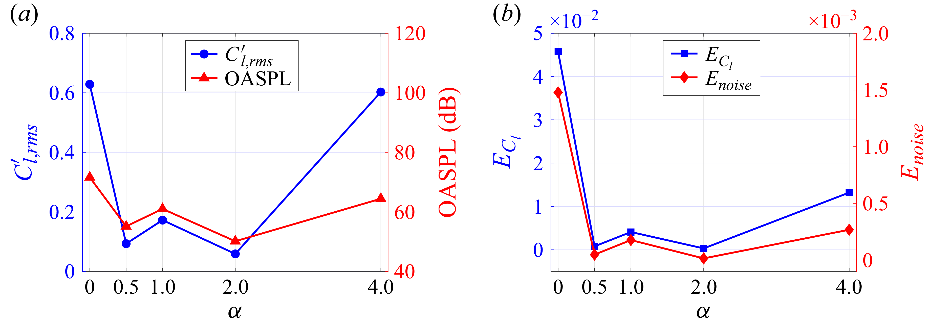
 α
 Cl,rms′
 ECl
 Enoise
 0.05

 C¯p
 Cp,rms′
 α
 α=0.5
 α=1
 α=2
 α=4

 Cp
 α
 α=0.5
 α=1
 α=2
 α=4

 Φpp,s
 St
 θ=90∘
 180∘
 270∘
 α=0.5
 1
 2
 4
 θ=90∘
 θ=180∘
 θ=270∘

 Φpp(ks,ωf)
 10log10[Φpp(ks,ωf)/pref2]
 0∘
 180∘
 360∘
 180∘
 s
 Uc
 U∞
 α=0.5
 1
 2
 4
 ksD
 St

 urms′/U∞
 vrms′/U∞
 x
 y
 x
 z
 y=0
 α=0.5
 α=1
 α=2
 α=4
 x
 y
 x
 z

 ω¯zD/U∞
 a
 b
 α=0.5
 α=1
 d
 α=2
 e
 α=4

 x/D=1
 a
 b
 α=0.5
 c
 α=1
 d
 α=2
 e
 α=4
 u
 Φuu
 v
 Φvv

 Λvv/D
 x/D=1
 y/D=0
 α=0.5
 1
 2
 4

 Ω
 Ω=0.52
 a
 b
 α=0.5
 c
 α=1
 d
 α=2
 e
 α=4
 ωxD/U∞
 α=4

 σ(x,t)
 x
 y
 α=0
 0.5
 1
 2
 4
 t0
 t0+Δt
 t0+2Δt
 t0+3Δt
 |T|=6.5D/U∞

 Rpv
 p′
 v′
 θ=90∘
 θ=270∘
 α=0.5
 1
 2
 4
 |Rpv|=0.60
 0.20
 α=0.5
 0.45
 0.15
 α=1
 0.20
 α=2
 4

 a
 b
 α=0.5
 c
 α=1
 d
 α=2
 e
 α=4
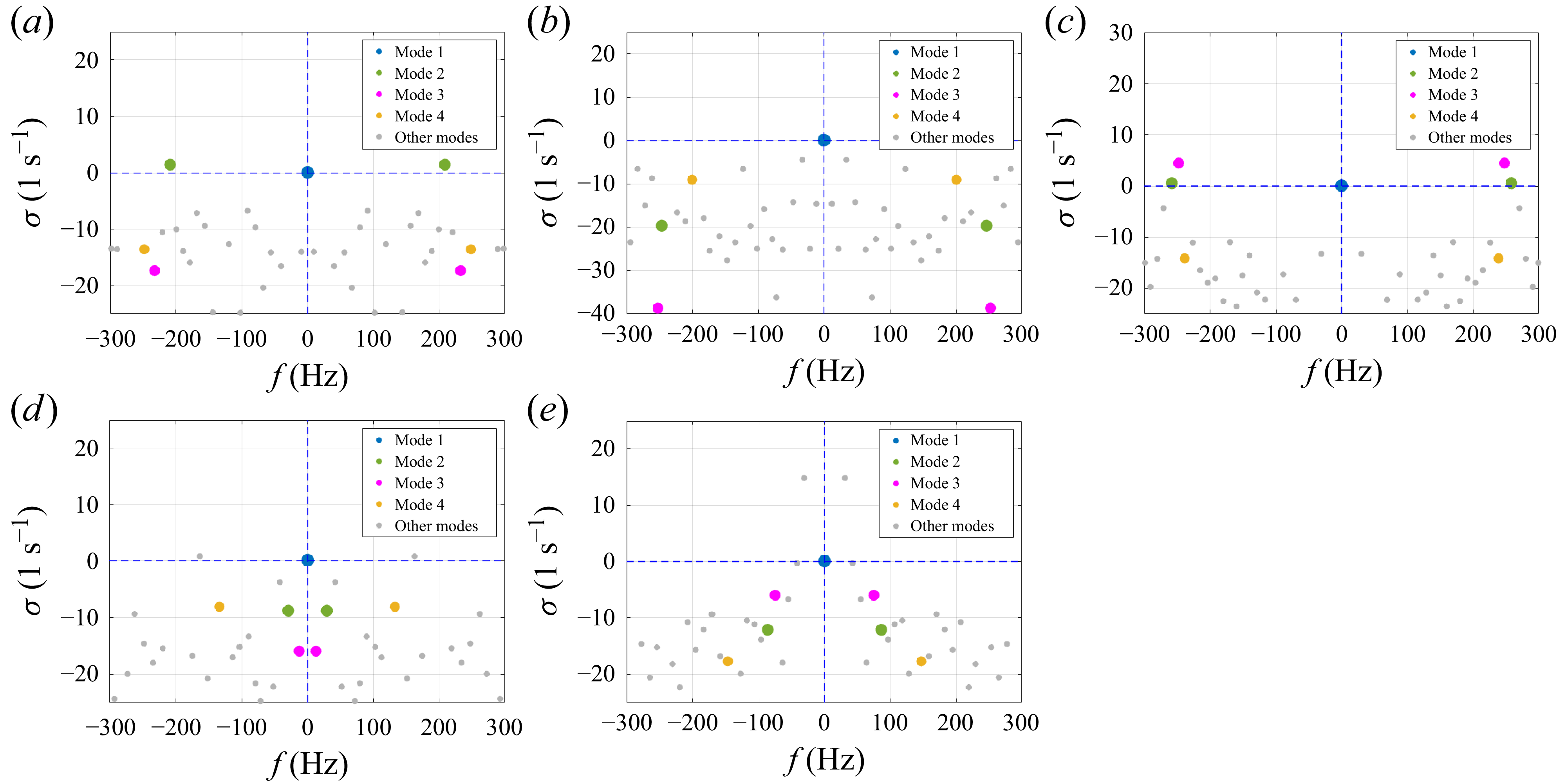
 a
 b
 α=0.5
 c
 α=1
 d
 α=2
 e
 α=4

 Pj
 St
 α=0.5

 Q
 ωzD/U∞
 Q=50000
 St=0.38
 Q=5000
 α=0.5
 1
 2
 4
 St
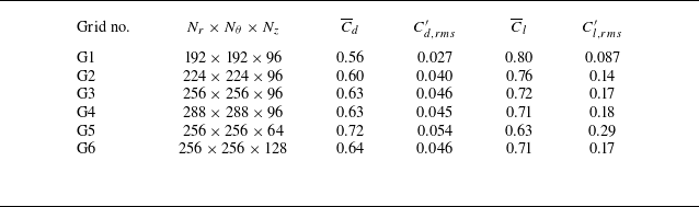
 α=1
 Re=4.7×10⁴
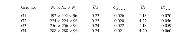
 α=2
 Re=4.7×10⁴

 α=2
 Re=4.7×10⁴
 u
 v
 x/D=0.8
 1.0
 1.5

 α=4
 Re=4.7×10⁴
 θ=90∘
 θ=270∘
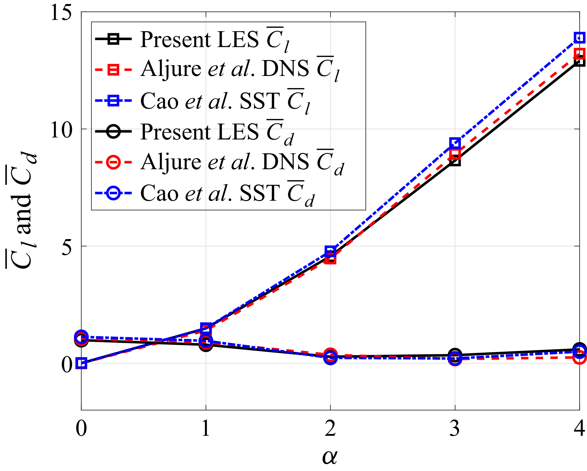
 Re=0.5×10⁴
 α
 C¯d
 C¯l


 SPL1/3
 α=0
 α=0.5


