Background and Framework

Reforms enacted by Maria Theresa in the late eighteenth century eliminated tariff barriers between the Austrian regions of the Habsburg Monarchy, forming the largest free trade area in Europe at the time, to the exclusion of the Kingdom of Hungary (Komlos Reference Komlos1983).Footnote ⁸ Although Austria and Hungary acted as one in foreign and military affairs, and even had a common currency, trade restrictions between the two regions of the Monarchy persisted well into the mid-nineteenth century.

The tariff wall consisted of a complicated structure of import and export taxes on various goods exchanged between the two regions. The consensus in the historical literature is that these levies, while potentially inhibiting to trade, were preferential relative to extra-imperial tariffs (Komlos Reference Komlos1983; Good, Reference Good1984). For instance, in the 1830s and 1840s, Hungarian wheat exports to Austria were charged a 7.5 percent tax, while foreign wheat paid 10.0 percent. On average, Hungarian goods imported into Austria were taxed at half of the rate levied on foreign goods. Imports of Austrian manufactures into Hungary were taxed considerably less at 3.5 percent, while Hungarian wool entered the Austrian market virtually duty free (Komlos Reference Komlos1983).

Because the Austrian Constitution prohibited internal trade restrictions, the tariff wall between Austria and Hungary dissolved when Hungary was formally incorporated into the Austrian Empire after the failed revolutions of 1848 (Eddie Reference Eddie1977). The customs union was officially created in 1850, but the years just prior to 1850 and the following two decades (roughly, 1848 to 1873) are generally known as a period of political and economic liberalization throughout the Monarchy (Eddie Reference Eddie1977; Komlos Reference Komlos1983; Good Reference Good1984). Internally, reforms included the emancipation of the serfs in 1848, the establishment of a central bank, and the abolition of the guild system in 1859 (Eddie Reference Eddie1967). Externally, Habsburg trade liberalization followed European trends during this era, engaging in tariff reductions and “liberal treaties” with England and Germany, which limited Austrian-specific duties and ad valorem taxes. The most notable of these are the tariff reductions of 1851, 1853, and 1865, the 1865 treaty with England, and the “Supplementary Convention” of 1869, which limited Habsburg-specific duties to agreed maximum ad valorem levels (Eddie Reference Eddie1977).

Ricardian trade theory predicts that countries specialize in the production of goods in which they have comparative advantage. Differences in production technologies or factor endowments make labor relatively more or less efficient in the production of certain goods, such that with the opening of trade countries specialize in the goods that they are relatively more efficient in producing (Costinot Reference Costinot2009). Throughout our analysis we assume that Hungary has the comparative advantage in agricultural goods, while Austria has the comparative advantage in forest and manufactured goods. Online Appendix Figure E1 supports this by showing that Hungary has a lower relative price for wheat (relative to wood) in the years prior to the customs union.

A simplified Ricardian framing predicts that after the customs union of 1850, Hungary should exchange agricultural goods for manufactured goods. To extend the prediction to land use, in the absence of significant and differential technological change in the years following the customs union, we expect more land to be allocated to agriculture in Hungary and less in Austria. Due to a lack of disaggregated trade data for the Habsburg Monarchy, we cannot specifically examine goods. Instead, we use highly disaggregated data on land as a production indicator, and examine trends in land use after the opening of trade. To support our analysis, we also explore aggregated trade and production statistics, which are not suited for formal analysis, but do support the trends found in our data.

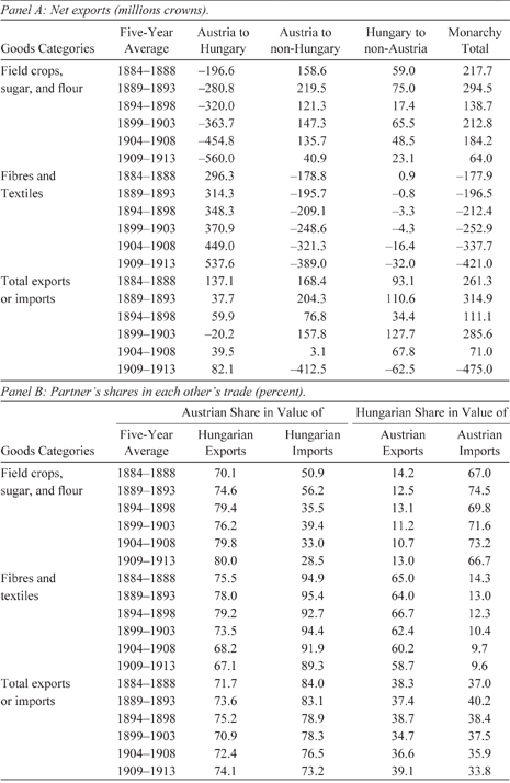
We first present summary statistics in Table 1 illustrating the interdependence and specialization in trade between Austria and Hungary over time. Ideally, we would like to examine trends in the data before and after the customs union. Unfortunately, however, while trade data for Austria is available in the period prior to the customs union, reliable data for Hungary only exists from the 1880s onward (Eddie Reference Eddie1989).Footnote ⁹ However, the data in Table 1 show clear patterns of interdependence and specialization between the two regions in the period between the 1880s and early 1900s—30 years after the establishment of the customs union. Panel A indicates that Austria sustained a trade deficit with Hungary in agricultural goods (field crops, sugar, and flour) and a surplus in manufactured goods (fibres and textiles), which steadily increased from 1884 to 1913. Moreover, when we examine each partner’s share in the other’s trade as a percent of the total value of imports and exports, similar patterns emerge. Panel B shows that the Austrian share in the value of Hungarian agricultural exports was 70.1 percent in the period between 1884 and 1888, increasing to 80.0 percent between 1909 and 1913. Over the same period, the Austrian share in the value of Hungarian agricultural imports declined from 50.9 percent in the period between 1884 and 1888 to 28.5 percent between 1909 and 1913. Hungarian imports of manufactures came almost entirely from Austria, whereas the Austrian share of Hungarian imports declined slightly from 94.9 percent in 1884–1888 to 89.3 percent by 1909–1913. Moreover, Hungary was the principle export market for Austrian manufactures, with the Hungarian share in the value of Austrian fibres and textiles exports representing 65.0 percent in 1884–1888, declining slightly to 58.7 percent by 1909–1913.

Table 1

Structure of Austro-Hungarian Trade

Source: Eddie (Reference Eddie1989).

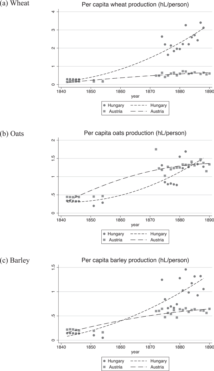
The observed changes in flows of goods are consistent with the production data from nineteenth century Habsburg statistical records.Footnote ¹⁰ Figure 1 shows per capita production over time averaged across provinces in Austria and districts in Hungary, and fitted across time with a second degree polynomial. Two things are evident from these figures. First, there is no information on production between 1854 and 1872. Therefore, a contribution of our work is that we show changes in production indicators during this period. Second, the data that do exist show increased productivity (output per capita) in Hungary relative to Austria, particularly for wheat and barley, in the post-customs union period.

Figure 1

Austro-Hungarian Agricultural Production Specialization

Dots indicate averages of observations within Austria and Hungary by year, and lines are fitted second order polynomials. Sources: Tafeln zur Statistik der Österreichischen Monarchie (Austria, Statistisches Central-Comission 1865), Statistisches Jahrbuch der Österreichischen (Austria, Statistisches Central-Comission 1881), Östrreichisches statistisches Handbuch fur die im Reichsrathe vertretenen Konigreiche und Lander (Austria, Statistisches Central-Comission 1914), Magyár Statistikai Közlemények (Orszagos Magyar Kir 1911), and Magyár Statistikai Évkönyv (Orszagos Magyar Kir 1918).

While summary statistics using aggregated data are illuminating, they suffer from significant measurement error, a high proportion of missing observations in key years, and the fact that identification of specialization relies on comparing differences in time trends across large areas, whose counterfactuals are time trends in very different places in Austria. Recent work by Schulze (Reference Schulze2000, Reference Sandgruber2007) carefully constructs per capita GDP measures for Austria and Hungary from 1870 to 1913, considering physical and human capital stock and growth. The data show that, consistent with the trends noted earlier, the agricultural sector was far more productive in Hungary than in Austria and was the main driving force of Hungarian economic growth between 1870 and 1913 (Schulze Reference Schulze2000, Reference Sandgruber2007). Linking these trends with the creation of the customs union requires counterfactuals over time and across nearly identical geographic spaces. We examine disaggregated data in order to compare places with similar geographies and observe tradeoffs in key land uses. In addition, the spatial detail of our data allows us to exploit heterogeneity that can reveal the mechanisms through which production evolved over the last half of the nineteenth century.

Data and Methodology

The main source of data for this study are maps from the Habsburg Monarchy’s Second Military Survey, which took place from 1806–1869 (Timár et al. Reference Timár, Molnár and Székeley2006). The First Military Survey occurred from 1763–1785 after the failed Seven Years War (1756–1763). Because the first survey expedition was plagued by a lack of precision, the Second Military Survey used more sophisticated cartographic techniques. It is important to bear in mind that the primary purpose of the Second Military Survey was just that—military. The Monarchy was under constant threat from outside incursion, and it was clear from the late eighteenth century that the Habsburgs saw mapping as an essential input into military organization. The maps produced by the military engineers were highly secretive—the results of the First Military Survey, for example, were kept hidden until the 1850s (Veres Reference Veres2015), and public access to successive military surveys was also forbidden.

Even though the Second Military Survey was not designed to assess production (unlike cadastral maps), it provided detailed information on land-use patterns across the region, and is the oldest reliable dataset providing wall-to-wall land-use data (Munteanu et al. Reference Munteanu, Kuemmerle and Bolitziar2014, Reference Munteanu, Kuemmerle and Keuler2015). The Second Military Survey also represents a major achievement in scientific and political knowledge. Building on the nineteenth century revolution in mathematics and science, it spurred the creation of a tremendous infrastructure for mapping, including building an engineer corps, astronomic observatories, map archives, and the regularization of practices across a diverse set of surveyors and mappers (Veres Reference Veres2015).

The study region encompasses what is known as the Carpathians Region of Eastern Europe and includes parts of the modern-day countries of Hungary, Poland, Slovakia, Romania, Ukraine, Czech Republic, and Austria. The underlying maps are at very fine scale—1:28,000 (each centimeter on the maps represents 0.28 kilometers). Complete digitization at this scale would have been prohibitively costly. Therefore, we did not digitize all the information in the maps, but rather a sample of points at the vertices of a 2-kilometer resolution grid over the entire study region, which contained around 80,000 data points. Each point in our sample grid was assigned the land-use classification from the point on the map directly below it (points have no area). Online Figure E2 illustrates an overlay of the grid, the sampled points, and a small part of the underlying historical map.

The land-use classifications used in this article include crops, pasture, forest and natural grasslands, wetlands, and urban land, although some of the maps had more extensive divisions. The classification represents categories that are both available across all maps and that roughly correspond to categories of production. We conduct our estimations on crops, pasture, and forest and natural grasslands because these are most closely related to traded production, and because observations of the other possible categories—wetlands and urban land—are scarce in the data and estimations are unlikely to be robust. The classification process and resulting dataset is described in Catalina Munteanu et al. (Reference Munteanu, Kuemmerle and Keuler2015). Because each point is classified into a unique land-use category, the outcomes that we analyze are binary.

GIS software was used to calculate the following characteristics for each point: slope, elevation, distance to nearest city, distance to nearest river, and whether or not the land had agricultural limitations according to the European Soil Database (ESDB, 2004). These limitations are determined by the scientists who created the ESDB. Some of the 17 possible agricultural limitations are: gravelly (more than 35 percent gravel), stony (presence of stones >7.5 cm, impracticable mechanization), lithic (hard rock within 50 cm), glaciers and snowcaps, frangipans, and excessively drained. The overlay of the points with district boundary maps from the Habsburg Monarchy provides boundary identifiers as well as distance to the Austria border. Finally, the statistical yearbooks of the Monarchy give population totals by district within Hungary for the years 1840, 1846, 1851, and 1857.Footnote ¹¹ We use these totals to calculate approximate population densities in the districts that we use for estimation, assigning the population density of the year closest to the year in which a point was mapped. Basic means and variations are shown in Online Table A1. Across the entire sample, the two dominant land uses are forest/grasslands and crops.

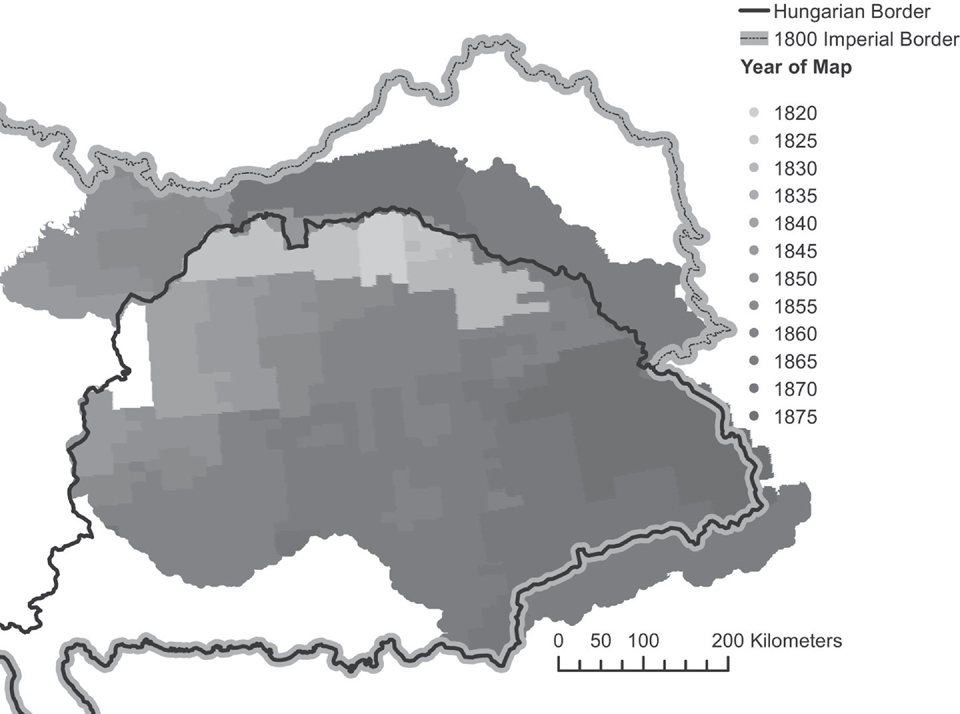
The main innovation of this article is to exploit the variation in the timing of mapping to try to isolate the effect of the customs union on land use. Figure 2 illustrates the temporal variation in the mapping process. The earliest mapping was clearly very strategic, focusing on the industrial and mining regions near the northern border, and then moving south and east.

Figure 2

Year in which The 2nd Military Survey was Conducted

Shading indicates approximate mapping year for each military map in the study sample. Source: Authors’ calculations using Timár et al. (2006) historical maps.

The variation in mapping dates across space allows us to employ a spatial discontinuity design, where the discontinuity in space proxies for a temporal discontinuity. This strategy is different than a standard spatial discontinuity approach, which usually measures the differences between “treatment” and “control” observations at the same point in time, but on different sides of a spatial treatment threshold (e.g., an administrative boundary, as in Dell (Reference Dell2010)). In our case, the “treatment” is time itself, since we are interested in the impact of a policy that has only temporal and not spatial variation. Ideally, we would like to analyze the same set of mapped data points before and after 1850 within Hungary and within Austria. However, since no single point was mapped both before and after 1850, we instead examine points that are arbitrarily close in space, but were mapped at different years. The timing of the map dates allows us to draw a line across space that represents a temporal discontinuity. The underlying assumption is that two points within a bandwidth of the 1850 mapping line are similar in their key determinants of land use (e.g., soil quality, slope, elevation, etc.), and that the placement of the line contains some element of random variation.

The non-random nature of mapping in general makes it difficult to argue time is uncorrelated with key determinants of land use, such as the inherent agricultural productivity of land. In order to assess whether or not the timing of mapping was related to agricultural productivity, we examine the distribution of mapping years for land with no agricultural limitations and land with some agricultural limitations. Figure E3 of the Online Appendix demonstrates that there was some tendency to map land with no limitations (better land) earlier, although it is also clear that for almost all time periods, both types of points exist. This means that when we run a regression that controls for whether or not a point has limitations, there are always sufficient observations to make comparisons across land of different qualities. Furthermore, if it is the case that the government mapped more productive lands first, then average agricultural productivity would decrease with the time variable in our sample. Given that more productive land is more likely to be used in agriculture, if we then compare land use before and after 1850, the fact that land mapped after 1850 is slightly less productive means that in the absence of any policy change, we would be more likely to observe decreases in the presence of agricultural land use over time. If the policy causes agricultural production to increase, then our estimation is likely to understate this impact.

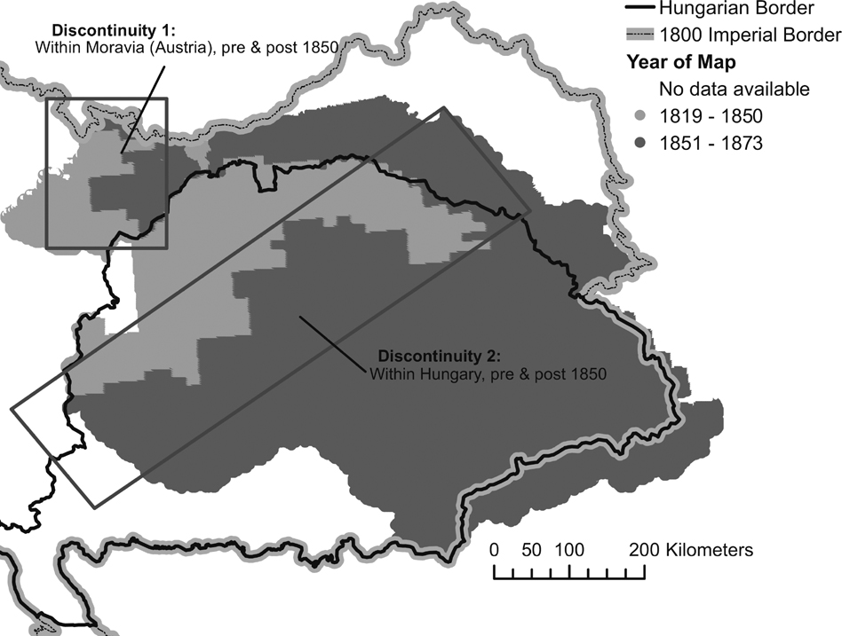
To limit the impact of variation in underlying geophysical characteristics that affect land productivity across space, our main strategy exploits the immediate areas along the line of maps before and after 1850. Figure 3 highlights the potential areas of analysis. The light grey areas in the figure indicate maps made before 1850, and the dark grey areas maps made after 1850. The black rectangles highlight two potential sources of variation: in Austria, before and after 1850, and in Hungary, before and after 1850. We will focus our analysis on the latter because this area has a sufficient number of districts within which there is temporal mapping variation. Discontinuity 1 provides only qualitative results, since Austria had only one district, Moravia, that was mapped before and after 1850.

Figure 3

Spatial-Temporal Discontinuities

Dark grey indicates areas mapped after 1850 and light grey before. The black boxes highlight the approximate regions of interest for data analysis. Source: Authors’ calculations using Timár et al. (2006) historical maps.

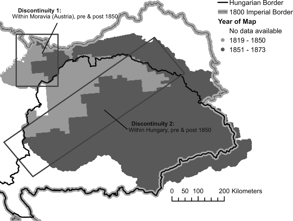
Our sample is defined by the region with maps created between 1840 and 1860, and within 40 kilometers of the discontinuity. The location of these maps is indicated by the rectangles on the map. We also check the robustness of this distance by using windows of 20 and 30 kilometers. By focusing on a narrow band of land around the mapping dates of interest, we hope to minimize geographic differences that might drive large scale changes in measured land use across space, as would occur, for example, if we compared lowlands, mapped in the earliest survey years, with high mountain vegetation of the Carpathians, which were mapped in the latest years of the survey. This approach is similar to recent articles with a European focus by Peter H. Egger and Andrea Lassmann (Reference Egger and Lassmann2015) and Pauline Grosjean and Claudia Senik (Reference Grosjean and Senik2011), who use spatial discontinuities with analysis windows of 50 and 25 kilometers, respectively.

The key outcomes are land-use dummy variables (y_ik ) for point i in district k: crops, pasture, and forest. The identification of the impact of the customs union comes from a combination of an indicator variable equal to one if mapping was done after 1850 and zero otherwise (D_ik ), and its interaction with a linear time trend set to zero at 1850 (T_t ). The estimation also contains a vector of control variables X_ik , the elements of which are ruggedness, agricultural potential, distance to nearest river, distance to the Hungarian border, and distance to the 1850 discontinuity line. We also include a quadratic of distance to the 1850 discontinuity (x_i (d)), as well as district fixed effects (γ_k ).Footnote ¹² In some specifications we also include the log transformation of the approximate district/year population density. The standard errors (ε_ik ) are clustered at the district level. The basic estimation equation is thus:

(1) ${y_{ik}} = {\alpha _0} + {\alpha _1}{D_{ik}} + {\alpha _2}{D_{ik}}{T_t} + {\alpha _3}{T_t} + \beta \cdot {X_{ik}} + \omega {x_i}(d) + {\gamma _k} + {\varepsilon _{ik}}$

All of the outcomes are binary, and we estimate this equation as a linear probability model using OLS.Footnote ¹³ The key assumptions underlying a causal interpretation of α ₂ are: (1) that individuals could not manipulate their position on either side of the temporal discontinuity and (2) that, conditional on controlling for smooth measures of distance and time, there are no omitted variables that are changing in the same way as D_ikT_t and thus driving the result. These are equivalent to the assumptions required for a standard regression discontinuity design (Lee and Lemieux Reference Lee and Lemieux2009), and we present evidence that they hold in the following section.

Because our discontinuity is both spatial and temporal, we require that individuals not change their behavior in anticipation of mapping. Anticipatory behavior alone should not be problematic if it is similar across time periods—for example, if people always anticipated that they would have improved tenure after mapping. However, it could threaten the identification strategy if the reasons for this anticipatory behavior were changing over time. The secretive nature of the mapping (discussed earlier) minimizes our worries about this problem. Furthermore, cartographic history of the Habsburg Military Surveys definitively establishes that the maps were made by a highly trained corps, that they were of predetermined sizes, and that more militarily sensitive areas were mapped first (Veres Reference Veres2015). The starting reference point for mapping was Vienna (Timár et al. Reference Timár, Molnár and Székeley2006). Because map sheets within Hungary were uniform in size, the location of the edges of these sheets is exogenous to local conditions. However, it could still be the case that mapping of an entire sheet was accelerated or slowed by local conditions. Because of this uncertainty, the robustness checks section presents a variety of estimations, including a test for anticipatory behavior and an estimation of the necessary correlation of an omitted variable that might overturn our results.

Discontinuity Summary Statistics

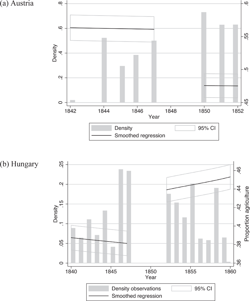
We begin by presenting graphs of one of the key outcomes in our data—the change in seasonal crops over time across our two within-country discontinuities. The vertical axis on the right side of Figure 4 shows the average values of outcome variables in Hungary and Austria, together with smoothed polynomial regressions estimated separately over the pre- and post-1850 periods for Austria (Figure 4a) and Hungary (Figure 4b). The bars, which correspond to the vertical axis on the left side of the figure, show the density of the data (the relative frequency of observations) for each year. The figures are consistent with the predictions: agriculture decreases in Austria and increases in Hungary, and it appears that the increases may be increasing over time (Figure 4b).

Figure 4

Discontinuities for Crops

The figures show kernel-smoothed regressions before and after 1850, where the dependent variable is an indicator for whether the point was used in agriculture in a given year. The densities show the distribution of the data across years, thus indicating the proportion of observations used in the regression in each year bin. Source: Authors’ calculations using Timár et al. (2006) historical maps.

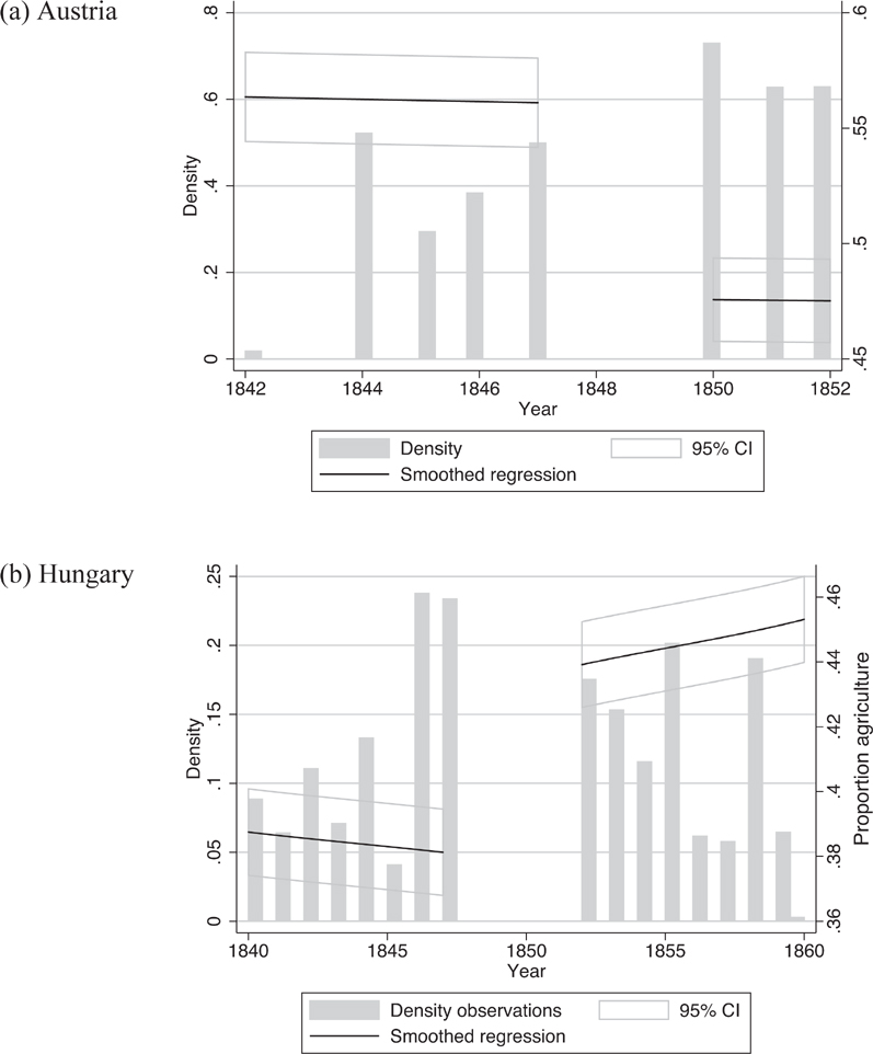
The figures highlight the weakness of the data for the within-Austria (Moravian) sample. In Austria, in addition to having all the data located in one province, there are very few years of observations after 1850. Because there is no provincial level variation in our Moravian data, and also because of the limited post-1850 data, we take these results as merely suggestive.

Trends in aggregate statistics for Austria available in Roman Sandgruber (Reference Sandgruber1978), which record increases in forest and crop land over the time period that we study, seem to potentially conflict with our findings in Figure 4.Footnote ¹⁴ However, while the Sandgruber (Reference Sandgruber1978) data is generally respected for its accuracy and scope, specific statistics pose challenges because they: (a) have been aggregated from various sources with little explanation of the methods and assumptions used to aggregate the data, (b) are available at only five discrete points in time,Footnote ¹⁵ (c) cannot take into account variation in land quality, and (d) may confound global trends with local causality. Nonetheless, we attempt to reconcile our suggestive findings with existing data sources by exploring land-use trends for Austria using aggregated data available in the Habsburg statistical yearbooks.Footnote ¹⁶ While these data also suffer from some of the same problems as the Sandgruber (Reference Sandgruber1978) data, there is potential insight to be gained from examining trends over a longer time period.

We fit quadratic polynomials to the data for Austria and for Moravia between 1830 and 1880 and examine trends in cropland and forested areas as a proportion of total provincial area. We expect to see a break in land-use trends before and after 1850. Note, however, that a classic regression discontinuity approach requires large samples around the discontinuity, which are not available in the aggregated yearbook data.Footnote ¹⁷

With this caveat in mind, the results presented in Figure E6 of the Online Appendix show no significant break in trends for crop or forested land around 1850 for Austria as a whole or for Moravia. In fact, they show almost no variation at all (note the limited range of the y-axis). We interpret these findings as evidence of the difficultly in precisely estimating the impact of the customs union without a proper counterfactual or highly disaggregated data. Taken together with our suggestive evidence for Moravia in Figure 4 we conclude that, at the very least, there were likely heterogeneous impacts of the customs union throughout Austria that are difficult to measure without detailed data.

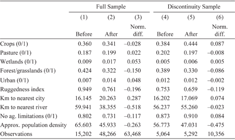
In addition to the visual discontinuities presented in Figure 4, we examine the summary statistics of outcomes and covariates across the temporal discontinuity within Hungary. Table 2 shows means, variances, and normalized differences across the 1850 cutoff for both the full sample of points (columns (1) and (2)) and the sample that is restricted to within 40 kilometers of a discontinuity (columns (4) and (5)).Footnote ¹⁸ The table also contains normalized differences of outcomes and covariates across the discontinuity (columns (3) and (6)).

Table 2

Sample within Hungary

The full sample includes all points mapped within Hungary. The discontinuity sample is limited to points mapped between 1840 and 1860 within 40 kilometers of the 1850 map line.

Source: Authors’ calculations using dataset described in Data and Methodology.

We observe slight decreases in the proportion of cropland and forest (Table 2), and increases in pasture and wetlands in the full sample. When we limit the sample to the discontinuity (columns (4) and (5)) we observe much less variation across covariates—for all control variables, the normalized differences between covariates in the before and after 1850 sample substantially decrease. In addition, in the discontinuity subsample, cropland now appears to increase substantially over time in Hungary rather than decrease.

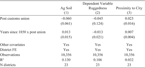
Because of our discontinuity strategy, it is important that we assess whether there are jumps in key covariates at the discontinuity threshold that indicate that there might be omitted variables driving the result. Table 3 shows the same regression specification that we employ for our main results, substituting as dependent variables some of the key covariates included in the estimation: if the point has no agricultural limitations, ruggedness, and proximity to the nearest city (1/(km to nearest city)). The “post customs union” variable then measures if there is a discrete jump in the value of this variable, conditioning on all the other covariates in the regression, and the interaction between post-union and time assesses whether or not the slope of the covariate also changes systematically across time after the establishment of the customs union. Out of the three outcomes, only proximity to nearest city is marginally significant after 1850. In particular, there is a positive and marginally significant (at the 15 percent level) coefficient on the interaction between post-union and time. However, the magnitude of this effect is quite small—less than 1/10th of a standard deviation of the proximity to city measure.

Table 3

Test of Covariate Discontinuity

^* p< 0.10

^** p<0.05

^*** p < 0.01.

Unit of observation is the point. Standard errors are in parentheses and are clustered at the district level. These are partial results using the sample within 40 km of the 1850 discontinuity. Other covariates include ruggedness, an indicator for agricultural soil, proximity to city, proximity to river, a quadratic of km to discontinuity, years since 1850, and ln(km to border with Austria).

Source: Authors’ calculations using dataset described in Data and Methodology.

Estimation Results

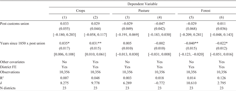
In Table 4 we show estimations for our main subsample, using the specification given in equation (1). There are significant and fairly large increases in cropland and decreases in forest/grasslands, while changes in pasture area are not statistically different from zero. The precision of the estimates increases with the addition of covariates, but does not substantially change their magnitude. For crops, the point estimate of 0.031 for the coefficient on the interaction between years since 1850 and the post-1850 indicator variable, relative to the baseline of 0.38 (column (4) of Table 2), implies that after 1850 crop area increased by 8 percent per year. The parallel impact on forest presence is about 6 percent given the baseline of 0.39.Footnote ¹⁹ Table 5 presents the results with standard errors clustered at the district level. Our small number of clusters (23) is somewhat problematic. However, when we estimate the standard errors using wild-bootstrap clustering (Cameron, Gelbach, and Miller Reference Cameron, Gelbach and Miller2008), we find equivalent significance levels (95 percent confidence intervals shown in square brackets in table).

Table 4

Impacts of Customs Union in Hungary

^* p< 0.10

^** p< 0.05

^*** p < 0.01.

Unit of observation is the point. Standard errors are in parentheses and are clustered at the district level. These are partial results using the sample within 40 km of a mapping border. All estimates include years since 1850, a quadratic of distance to discontinuity, and ln(km to border with Austria). Other co variates include ruggedness, an indicator for agricultural soil, proximity to city, and proximity to river. Ninety-five percent wild bootstrap clustered CIs in [].

Source: Authors’ calculations using dataset described in Data and Methodology.

We interpret these findings as causal evidence of the effect of the customs union on promoting specialization in agriculture in Hungary. To extrapolate these findings into evidence of changes in productivity from a reduction in trade barriers would require us to make assumptions about the relationship between land, capital, and labor that are beyond the scope of this article. Nonetheless, in the event that agricultural yields remained the same or increased due to technological progress, these estimates could represent a lower bound for the increase in production resulting from the customs union. However, they might also overstate the impact if it is the case that the extensification of agriculture resulted in moving production to land with lower inherent productivity. To assess whether or not this is the case, we examine the distribution of our inherent land productivity variable by year, for the land which was classified as agricultural in our sample during the post-union period. We observe that generally, agricultural land tends to fall into the category of having “no agricultural limitations,” and that if there is any time trend in this variable at all, it appears that higher-quality land is coming into production over time (see Figure E5 in Online Appendix).

At first glance, the results in Table 4 seem at odds with previous findings in the literature, namely Komlos (Reference Komlos1983) who argues that Hungarian per capita grain production did not differ quantitatively before and after 1850.Footnote ²⁰ Rather, Komlos argues, increased demand by Austrian consumers was the primary determinant of the growth in Hungarian grain production between 1828 and 1870 (Komlos Reference Komlos1983). However, due to the aggregated nature of the data, one may wish to interpret Komlos’ findings with caution.Footnote ²¹ Nonetheless, the argument that demand from Austrian consumers drove production patterns in Hungary does not contradict our findings. Prior to the customs union, Hungarian wheat imports to Austria were taxed at 7.5 percent, making a reduction to 0.0 percent a significant change. After 1850, Hungarian agricultural exporters were in an improved position to access increasing demand in Austria that was less accessible to foreign competitors, due to the high external tariffs surrounding the Habsburg customs union (Schulze Reference Sandgruber2007). It is therefore entirely possible that increased demand from Austria compounded the effect of a reduction in trade barriers on promoting growth in Hungarian agriculture.

Taken at face value, the Komlos’ (Reference Komlos1983) estimates do show a marked increase in the growth rate of per capita agricultural production in Hungary between 1869 and 1883, which Komlos argues is due in part to capital outflows from Austria after the 1873 Vienna stock market crash (Komlos Reference Komlos1983). It is possible that the changes in land use that we observe in the immediate period after the customs union were the predecessors to the subsequent changes in per capita production growth rates. Moreover, if it were true that the customs union had no effect on Hungarian agriculture and that trends were in place as early as 1828, then we should not observe any evidence of adjustments to factors of production—in our case, land—as a result of the customs union. The changes in land use that we observe in Table 4, however, are consistent with increased specialization in agriculture in Hungary after 1850. In the next section, we run a series of robustness checks to establish the validity of our main results.

Robustness Checks

Our main results are generally robust to including an interaction term between the post-union dummy and a quadratic of distance to the discontinuity, a test that allows the slope of the distance variable to change on either side of the discontinuity, and is in line with the recommendations of Guido W. Imbens and Thomas Lemieux (Reference Imbens and Lemieux2008) and David Lee and Lemieux (Reference Lee and Lemieux2009). We also check to see if our results are robust to narrower definitions of the discontinuity (20 and 30 kilometers). We observe impacts of slightly larger magnitude, with similar levels of significance to the 40-kilometer sample. These estimations are shown in the Online Appendix in Tables B3 and Table B4. We also include district by year trends. Our results remain similar with these time trends included, but we suspect that they introduce significant collinearity into the specification, given that they exploit very similar district-level variation to our treatment effect (see tables in Online Appendix C). Consistent with this observation, the magnitude of the point estimates with district by year trends is quite large.

While we hope that our strategy is not threatened by omitted variables, in the absence of a pure randomized experiment, there always remains the possibility that the inclusion of key omitted variables in the estimation might overturn the result. To assess this possibility, we follow the recommendations of Emily Oster (Reference Oster2017), who proposes a test based on the premise that changes in the coefficients of interest with the introduction of covariates can be informative about possible changes in estimation of treatment effects with the inclusion of omitted variables. The crux of the test is a conjecture about the covariance between the omitted variable and the treatment variable. One commonly made assumption is that the covariance between the omitted and treatment variable is equivalent to that between the observables and the treatment variable. This is known as the proportional selection assumption and implies a coefficient of proportionality (δ) equal to 1. We calculate the coefficient of proportionality that would overturn our results.Footnote ²² This coefficient is shown in the bottom row of Table 4 and Online Appendix Table B2. For cropland, the coefficient of proportionality required to overturn the interaction between post-union and the time trend result is over eight for the parsimonious specification, and almost ten for the full set of covariates. This indicates that an omitted variable would have to be substantially more correlated with the treatment variable than is the current set of observables in order to render the treatment effect equal to zero. The results for forest are similarly stable.

Table 5

Placebo Impact Test

^* p< 0.10

^** p<0.05

^*** p < 0.01.

Unit of observation is the point. Standard errors are in parentheses and are clustered at the district level. These are partial results using the sample within 40 km of a mapping border. Other covariates include ruggedness, an indicator for agricultural soil, proximity to city, ln(km to border with Austria), proximity to river, a quadratic of km to the discontinuity, and years since 1844. Ninety-five percent clustered bootstrapped CIs in [].

Source: Authors’ calculations using dataset described in Data and Methodology.

We also check to see whether it makes a difference to exclude districts that do not have meaningful variation in mapping dates, in other words, those that fall within the 40-kilometer border, but only have observations mapped either before or after the customs union. Online Appendix Table B2 contains estimates from the ten districts that have before and after 1850 maps within them. This is a relatively smaller sample, but the results remain robust with both clustered and wild-bootstrap clustering, and the estimated δ’s are again quite large.

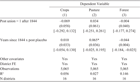
Additionally, we limit the Hungarian data to points mapped from 1840 to 1849, and move the discontinuity to 1844 to see if there are effects of the trade union where there should not be any. These results are shown in Table 5. There are no significant impacts of the placebo discontinuities, which is heartening, although we lose a considerable number of observations by removing the post-1850 data. Nonetheless, the data show no “anticipatory” effects, that is, land use did not change significantly in advance of the policy change. Another interpretation of this test is that—at least prior to 1850—mapping did not result in detectable changes in landholder production choices. The estimate on pasture is marginally significant but not robust.

We are also concerned that the results could be driven by population changes. As mentioned in the data description, the population data are available only at the district level and are limited. We have data for the years 1840, 1846, 1851, and 1857. Generally speaking, the data show population declining prior to 1850 and slightly increasing afterwards in the districts that we analyze. This could potentially explain the increase in agricultural production. However, in addition to being rather sparse, the quality of the population data prior to 1850 is suspect, given that Hungarians had a strong incentive to underreport population during the era leading up to the failed revolution of 1848.Footnote ²³ Nonetheless, when we include district population density in the year nearest to the map year, the agriculture results hold in all samples, though the result on natural vegetation becomes weaker (see Online Appendix D).

Heterogeneity by Distance to Border

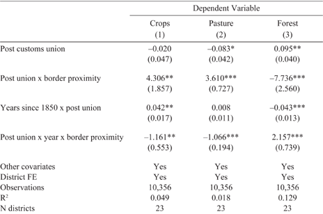
Finally, we test to see whether or not logical correlations exist between distance to the Hungarian border, land use, and the discontinuity. If it is the case that trade is the force driving the observed land-use change, we would expect it to be sensitive to travel costs. Most travel at this time was done by horse and carriage, or approximately 25 kilometers per day. Some trade took place on the Danube, but due to the mountainous, forested terrain throughout much of the empire, river and canal navigation did not attain the same significance as it did in other parts of Europe (Good Reference Good1984).Footnote ²⁴ To test the importance of travel costs, we interact the post-union and post-union time trend variables with a measure of proximity to the border between Austria and Hungary (specifically, 1/ km to the border).Footnote ²⁵ Table 6 shows the estimates from just the impact and interaction terms, and Online Figure E7 illustrates the total marginal effects and 95 percent confidence intervals calculated for distances up to 80 kilometers to the border (they remain flat thereafter). We observe that the significant increases in agriculture, and decreases in forest, are concentrated with less than 50 kilometers of the border.

Table 6

Impact of Customs Union by Distance to Austro-Hungarian Border

^* p< 0.10

^** p<0.05

^*** p < 0.01.

Unit of observation is the point. Standard errors are in parentheses and are clustered at the district level. These are partial results using the sample within 40 km of a mapping border. Other covariates include ruggedness, an indicator for agricultural soil, proximity to city, a quadratic for distance to discontinuity, proximity to river, and years since 1850. Border proximity is measured as 1/km to border.

Source: Authors’ calculations using dataset described in Data and Methodology.

Alternative Mechanisms

Implications and Conclusions

Our article tries to identify the impact of a reduction in barriers to trade on the distribution of production and land use. Using a modified spatial discontinuity approach with disaggregated data from historical maps, we show that the 1850 customs union between Austria and Hungary resulted in a significant reallocation of production. Austria reduced its agricultural land use, while Hungary increased the amount of cropland at the expense of forest. We rule out that the adjustment in agricultural land in Hungary was part of a trend that began prior to the customs union, that it was a result of the emancipation of the serfs which occurred around the same time, or that it stemmed from differential adoption of agricultural technology. We also show that the estimates are sensitive to distance from the border between the two regions, thus more precisely identifying the trade mechanism.

We interpret these results as specialization induced by the lowering of tariffs. The benefits of this specialization, however, may have been uneven. While we do observe some decrease in agricultural land in Austria immediately after the customs union, recent literature suggests that Austria did not fully specialize in manufacturing. Schulze (Reference Sandgruber2007) shows using aggregated census data that Austrian aggregate productivity growth was stifled by a slow exit of workers from the agricultural sector and low rates of capital formation between 1870 and 1910. Moreover, while capital intensity increased rapidly in Austria between 1890 and 1910, it did not translate into labor productivity growth in the manufacturing sector. By 1910, Austria’s per capita GDP was just 53 percent of Germany’s, while Hungary’s stood at 40 percent (Schulze Reference Sandgruber2007).

Our findings for Hungary support the historiography that documents a dominance of the agricultural sector in Hungary throughout the nineteenth and early twentieth centuries (Komlos Reference Komlos1983; Good Reference Good1984; Schulze Reference Schulze2000, Reference Sandgruber2007). Our results are also in line with observations of interdependence in trade between Austria and Hungary during the last 40 years of the Monarchy’s reign in which Hungary maintained a trade surplus in agricultural goods with Austria, while Austria maintained a trade surplus in manufacturing goods with Hungary (Eddie Reference Eddie1989). The present article contributes to the historical discussion by providing causal evidence that this specialization was catalyzed by the customs union.

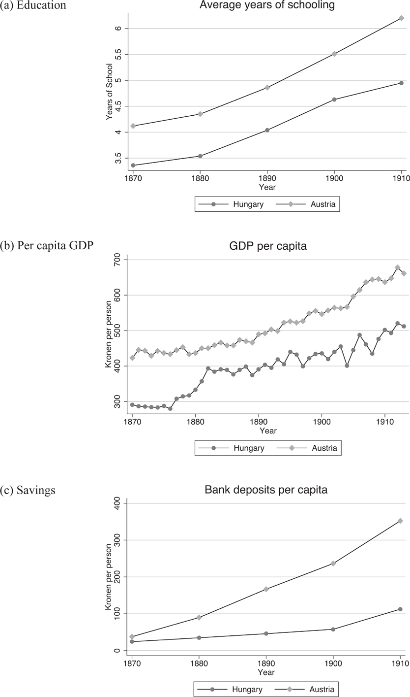
In the long run, there could be broader economic implications resulting from specialization, particularly in agriculture. When compared to manufacturing, there is evidence that the returns to education for agricultural workers are lower (Goetz and Rupasingha Reference Goetz and Rupasingha2004; Jolliffe Reference Jolliffe2004). Therefore, in the event that one region specializes in agriculture, long-run investment may be stifled, resulting in negative long-run economic outcomes. Recent work shows that per capita GDP grew substantially faster in Hungary than Austria from 1870 to 1913, and that growth in value-added per worker across agriculture, manufacturing, finance, and transport were much higher in Hungary over this period, as well (Schulze Reference Schulze2000, Reference Sandgruber2007).Footnote ²⁷ However, there is some suggestive evidence that this growth was not coincident with long-run investment. It may be the case that Hungary’s specialization in agriculture created disincentives to invest in human capital and other economic fundamentals. Figure 5 shows that the average years of schooling was consistently lower in Hungary than in Austria and increased at a slower rate over the latter nineteenth and early eighteenth centuries. In addition, while per capita GDP grew at a higher rate in Hungary than in Austria, per capita income levels remained higher in Austria than Hungary over this period.

Figure 5

Long Run Investment Outcomes

Sources: Schulze (2007) for panels (a) and (b). Tafeln zur Statistik Österreichischen Monarchie provided by David Good for panel (c).

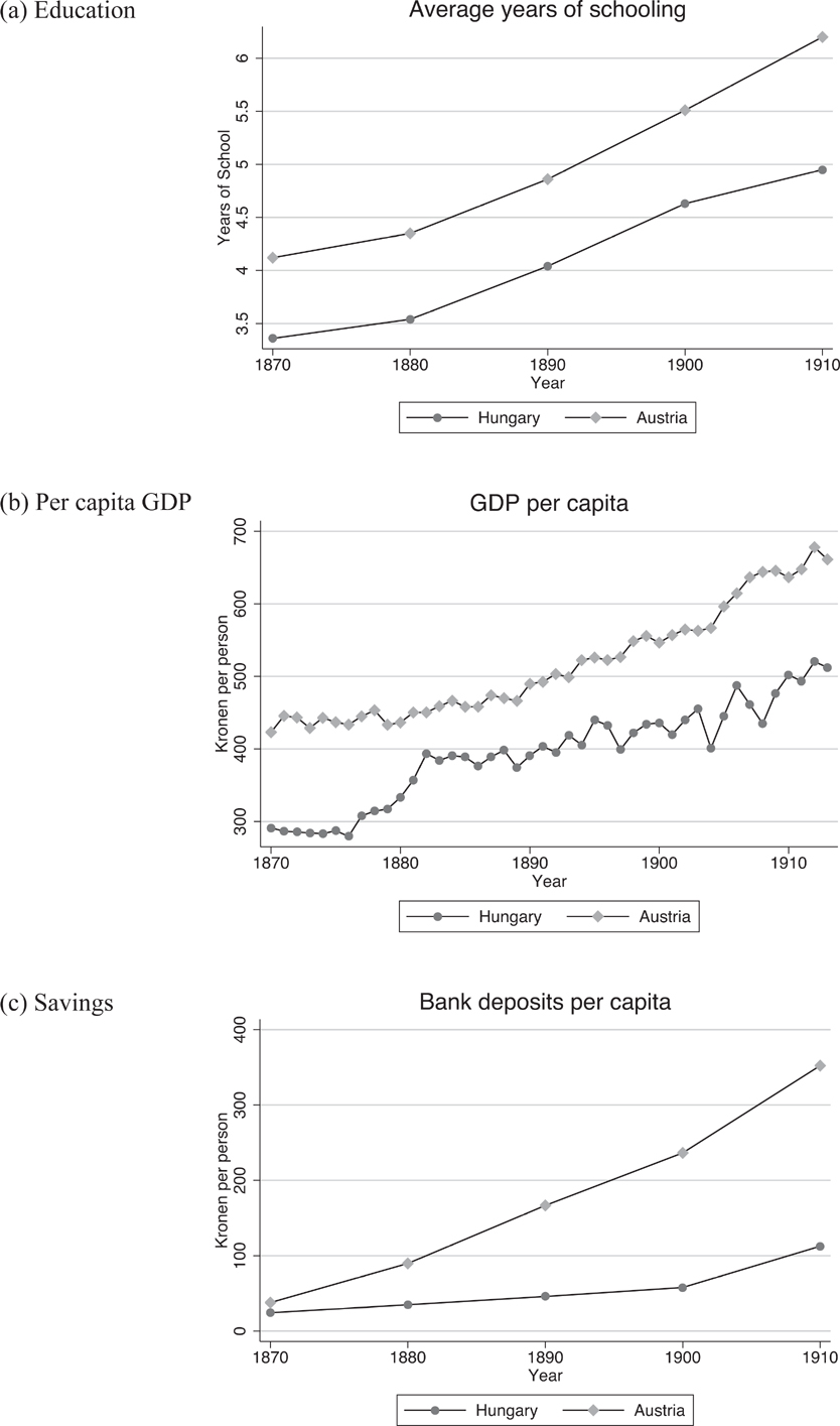
Lastly, per capita savings—an important determinant of macro-level investment and economic growth—started out at similar levels for Austria and Hungary in 1870, but quickly diverged over the next 40 years, with Austria’s savings becoming increasingly greater than Hungary’s.

In addition to contributing to the historical debate, our findings add to the broader discussion of the relationship between globalization and the environment. In the context we examine, forest was sacrificed in favor of agriculture. Because of this, our work also contributes to the ongoing discussion regarding the impacts of trade liberalization on natural resource use (see Copeland and Taylor (Reference Copeland and Taylor2004) for a review). While there are a significant number of theoretical articles on this issue,Footnote ²⁸ the majority of the empirical work relies on cross-country estimations where endogeneity concerns are very difficult to address and results are contradictory.Footnote ²⁹ A few articles use within-country estimates where it is difficult to separate out general time trends (Barbier Reference Barbier2000; Faria and de Almeida Reference Faria and de Almeida2013). Our approach is unique in its ability to focus on the impacts of trade openness on various types of land use, including forest, pasture, and agriculture. However, we are unable to measure the net effect of this activity, that is, the amount of forest which grew back in Austria as it was cut down in Hungary. This is both because we do not have data for the entire Austrian region of the Monarchy, but also because our identification strategy relies on a local treatment effect. The true externality effects of this reallocation of activity could only be assessed were we able to examine the value of the regrown forest relative to that of the forest lost to agriculture.

Using highly disaggregated data and a clean identification strategy, we are able to make sound claims about the effect of trade liberalization on land use. We find evidence of specialization with the elimination of trade barriers that resulted in forest loss in Hungary, which had a comparative advantage for agriculture. The impact of these tradeoffs in the long term remains an interesting area of inquiry for future work.