Nomenclature
- a
-
acceleration
-
 $t_f$
-
terminal time of the engagement
- r
-
capture radius of the defender
- R
-
relative distance
- u
-
control input
- V
-
velocity
- z
-
zero-effort miss
-
$\gamma$
-
flight path angle
-
$\gamma _f$
-
expected terminal flight path angle
-
$\lambda$
-
line-of-sight angle


1.0 Introduction
In nature, it is a common phenomenon that predators chase their prey. Similar scenarios also appear frequently in practical engineering applications, such as attacking missiles pursuing manoeuvring targets [Reference Wang, Lu, Huang and Zuo1–Reference Wang, Fu, Fang, Zhu, Wu and Wang3], fighter jets chasing enemy aircraft [Reference Shin, Lee, Kim and Shim4] and torpedoes attacking ships [Reference Boyell5]. All of these phenomena can be regarded as instances of pursuit-evasion games, where the agents try their best to achieve their respective objectives.
Differential game theory, originally introduced by Isaacs [Reference Isaacs6], is a powerful tool for solving pursuit-evasion problems. In differential game theory, cost functions are presented, which can reflect the objectives of the agents. The Hamiltonian function is then constructed, and the minmax technique is used to solve the saddle point or equilibrium solutions, which are taken as the agents’ guidance laws, enabling them to try to achieve their respective maximum guidance performance. According to the cost functions, differential games can be classified into two categories: qualitative differential games and quantitative differential games.
In qualitative differential games, the cost functions take only finite values. Based on qualitative differential game theory, the necessary winning conditions for each agent can be derived, and the corresponding guidance law can be designed. The whole state space is partitioned into distinct regions by barrier surfaces [Reference Başar and Olsder7]. Each region corresponds to a necessary condition of an agent winning the game if the system’s initial states lie within that region. The scenario of a missile intercepting a target was investigated in Reference [Reference Turetsky and Shinar8], where the Hamiltonian functions are derived and the min-max principle is used to obtain the guidance laws of the vehicles. In Reference [Reference Pontani9], a genetic iterative algorithm was applied to obtain the necessary winning conditions of the respective agents. A scenario in which multiple attackers jointly pursue a single target was investigated in Reference [Reference Deng, Zhang, Yan, Shi and Zhong10], where the cooperation among the pursuers is taken into account. In Reference [Reference Garcia, Casbeer, Moll and Pachter11], the constant flow field was introduced into the pursuit-evasion game. The study demonstrates that such a field can be neglected when all agents are moving, but it must be considered when there are stationary agents involved. In Reference [Reference Sun, Tsiotras and Yezzi12], the pursuit-evasion game was studied in three-dimensional space. The optimal evasion strategies are designed based on the qualitative differential game theory in References [Reference Zhang, Zhang, Shi, Huang, Bi, Ye and Wang13–Reference Li, Wang, Sun, Zhang and Xie16]. The orbital optimal evasion problem was solved in Reference [Reference Zhang, Zhang, Shi, Huang, Bi, Ye and Wang13], and the pursuit-evasion game with two heterogeneous players was investigated in Reference [Reference Li, Wang and Xie14]. An approximate analytical approach was proposed to solve the optimal evading strategy in Reference [Reference Jia, Ye, Xiao and Sun15], where the two-point boundary value problem is solved by the Hamiltonian min-max technique. A multiplayer pursuit-evasion game was investigated in Reference [Reference Li, Wang, Sun, Zhang and Xie16], where distributed optimal evading strategies are designed. A three-party pursuit-evasion game (also referred to as a target-attacker-defender (TAD) game) was investigated in Reference [Reference Liang, Deng, Peng, Li and Zha17], which is more complex than the traditional two-party one. The three-party game involves an attacker party, a defender party and a target party. Each party involves one or multiple agents. The attacker party aims to capture the target party. The defender party attempts to intercept the attacker party and assist the evasion of the target party. The target party seeks to evade the attacker party. The TAD game was further investigated in Reference [Reference Liang, Deng, Lu and Chen18], where the capture radius of the attacker is taken into account. In the above literature, the dynamics of the agents are modelled as first-order integrators, with the agents’ velocities treated as the control inputs. However, in physics, changes in velocities are generated by accelerations. Thus, the first-order dynamic model is overly simplistic and deviates significantly from the real-world one. To address this, second-order double integrator models for the agents are adopted in References [Reference Sergey and Shaul19–Reference Sun, Qi, Xiao and Lin21], where accelerations are treated as the control inputs. The necessary initial conditions under which each player can win the TAD game are respectively analysed. Nevertheless, the cooperation between the defender and the target is not considered, resulting in conservative results.
In practical scenarios, when the capture is possible, the pursuer often aims to minimise the terminal distance from the evader to improve the effectiveness of capture. Quantitative differential game theory is well suited to address such objectives. In quantitative differential games, the cost functions typically include the terminal distances between the agents (norm-bounded differential games), or the combinations of the terminal distances and weighted control efforts (linear-quadratic differential games). By optimising the cost functions, an equilibrium solution can be obtained and adopted as the agents’ guidance strategies, ensuring that each agent’s guidance performance is maximised. In Reference [Reference Shinar and Shima22], the authors studied a missile-target engagement scenario, where the Riccati equations are derived, by solving which the optimal strategies of the vehicles are obtained. Terminal constraints of the attacker were taken into account in Reference [Reference Shaferman and Shima23]. References [Reference Liu, Dong, Li and Ren24] and [Reference Shaferman and Shima25] investigated cooperative pursuit-evasion games involving multiple attackers and a single evader. Specifically, system uncertainties were considered in Reference [Reference Liu, Dong, Li and Ren24], and terminal constraints on the attackers were considered in Reference [Reference Shaferman and Shima25]. A pursuit-evasion problem in the three-dimensional engagement was presented in Reference [Reference Chen, Li and Mao26], where optimal pursuit and evasion strategies are derived and applied to the unmanned aerial vehicle (UAV) engagement scenario. The quantitative differential game theory was first applied to a TAD game in Reference [Reference Perelman, Shima and Rusnak27], where both continuous and discrete Riccati equations are given and solved, and the guidance laws are designed for both continuous and discrete dynamic systems. The three-party game was divided into two phases in Reference [Reference Liang, Wang, Wang, Wang and Liu28]. In the first phase, the attacker evades the defender, and the attacker pursues the target in the second phase. In Reference [Reference Chao, Wang, Wang and Yang29], a more reasonable cost function was proposed to better reflect the objectives of the respective agents. Reference [Reference Xie and Ma30] considered a scenario involving an attacker, multiple defenders and a target, considering terminal constraints for the defenders. Reference [Reference Shalumov31] investigated a more complex engagement scenario including multiple attackers, multiple defenders and a target. It is assumed that the number of attackers equals that of the defenders. The respective cooperation among the attackers and among the defenders is considered, and the guidance laws of all agents are given. The stochastic characteristics in the system modelling process were considered in Reference [Reference Li, Wang, Liu and Deng32], where guidance laws for all agents in a three-party game are designed based on stochastic differential game theory. Reference [Reference Liang, Wang, Liu and Liu33] focused on a two-versus-two engagement scenario and designed corresponding guidance laws for the agents. In Reference [Reference Wang, Yang, Wang and Chao34], the same scenario was addressed by dividing the engagement into multiple phases based on the predicted capture points, with respective cost functions and guidance laws designed for each phase.
This paper investigates a TAD game, with an attacker chasing a target and multiple defenders cooperatively capturing the attacker to protect the target. In the engagements between the attacker and the defenders, the attacker is required to maintain a distance greater than each defender’s capture radius to avoid being captured, which makes the attacker-defender engagement a qualitative process. On the other hand, in the engagement between the attacker and the target, the attacker aims to minimise the terminal distance from the target to improve the effectiveness of the capture, which constitutes a quantitative process. To address both aspects simultaneously, a hybrid differential game approach is proposed. Compared with the existing literature, the main contributions of this paper are summarised as follows.
-
(1) A hybrid differential game approach is proposed to solve the TAD game. Firstly, the qualitative differential game theory is used to derive the ranges in which the guidance commands of the attacker take values. Subsequently, the agents’ guidance laws are obtained based on the quantitative differential game theory, with the ranges obtained from the qualitative differential game treated as the feasible region for the attacker.
-
(2) In the qualitative differential game, the dynamics of the agents can be modelled as arbitrary-order dynamical systems. Different types of dynamical systems can all be described by the proposed dynamic model, which is more general compared with the first-order or second-order double integrator models commonly used in the existing literature.
-
(3) A class of segmented cost functions are proposed by combining the norm-bounded and linear quadratic cost functions. In the early phase of the game, linear quadratic cost functions are used to reduce the energy cost, while in the endgame, norm-bounded cost functions are used to enhance the guidance effectiveness. The proposed segmented cost functions can better reflect the objectives of the agents.
The rest of this paper is organised as follows. Section 2 gives the models of the TAD game and formulates the problem of this paper. Section 3 presents the hybrid differential game approach. Sections 4 and 5 respectively give the solution processes of the qualitative and quantitative differential games. Section 6 presents the applications of the proposed hybrid differential game approach, and Section 7 concludes this paper.
2.0 Dynamics and problem formulation
2.1 Dynamics of the game
Considering a TAD game with an attacker
 $U$
controlled by
 $u$
, multiple defenders
 $V_i$
controlled by
 $v_i$
and a target
 $W$
controlled by
 $w$
. The dynamics of the game are given as follows
 \begin{align} &\left \{ \begin{aligned} &\;\;\dot {\!x}_{\xi _i}=A_{\xi _i}x_{\xi _i}+B_{\xi _i}(u+v_i)\\ &y_{\xi _i}=L_mx_{\xi _i} \end{aligned} \right . \end{align}
 \begin{align} &\left \{ \begin{aligned} &\;\dot {\!x}_{\delta }=A_{\delta }{x_{\delta }}+B_{\delta }(u+w)\\ &y_{\delta }=L_px_{\delta } \end{aligned} \right . \end{align}
 \begin{align} &\left \{ \begin{aligned} &\;\dot {\!x}_{\eta _i}=A_{\eta _i}x_{\eta _i}+{B_{\eta _i}}{v_i}\\ &y_{\eta _i}=L_qx_{\eta _i} \end{aligned} \right . \end{align}
where
 $i=1,2,\ldots ,n$
. The dynamics of the games between
 $U$
,
 $V_i$
and
 $U$
,
 $W$
are respectively given by (1) and (2).
 $x_{\xi _i} \in \mathbb{R}^m$
,
 $x_{\delta } \in \mathbb{R}^p$
are the states of the systems.
 $u \in \mathbb{R}$
,
 $v_i \in \mathbb{R}$
and
 $w \in \mathbb{R}$
are the control inputs, i.e. the guidance laws of agents.
 $y_{\xi _i} \in \mathbb{R}$
and
 $y_{\delta } \in \mathbb{R}$
are the outputs.
 $A_{\xi _i} \in \mathbb{R}^{m \times m}$
,
 $A_{\delta } \in \mathbb{R}^{p \times p}$
,
 $B_{\xi _i} \in \mathbb{R}^{m \times 1}$
,
 $B_{\delta } \in \mathbb{R}^{p \times 1}$
,
 $L_m \in \mathbb{R}^{1 \times m}$
and
 $L_p \in \mathbb{R}^{1 \times p}$
are the matrices of the systems. There are multiple defenders in the game, thus some constraints (such as moving trajectory constraints) are necessary for defenders, the dynamics of which are given in Equation (3).
 $x_{\eta _i} \in \mathbb{R}$
,
 $v_i$
and
 $y_{\eta _i} \in \mathbb{R}$
are the state, the input and the output of the system.
 $A_{\eta _i} \in \mathbb{R}^{q \times q}$
,
 $B_{\eta _i} \in \mathbb{R}^{q \times 1}$
and
 $L_q \in \mathbb{R}^{1 \times q}$
are the matrices of the system.
Assumed that
 $\left |u\right | \leq \overline {u}$
,
 $\left |v_i\right | \leq \overline {v}_i$
and
 $\left |w\right | \leq \overline {w}$
, where
 $\overline {u}$
,
 $\overline {v}_i$
and
 $\overline {w}$
are positive constants representing the bounds of agents’ guidance laws. The game time involving agents’
 $U$
and
 $W$
is defined by
 $t_f$
, which represents the entire game time. During the period of
 $(0,t_f)$
, there exist the times
 $t_{f_i}$
 $(i=1,2,\ldots ,n)$
representing the game times between the agents
 $U$
and
 $V_i$
, respectively. It is assumed that the agent
 $V_i$
is not involved in the game after
 $t_{f_i}$
. The entire game can be divided into two phases. The first phase is during the period of
 $[0,t_m]$
, and the second one is during the period of
 $(t_m,t_f]$
, where
 $t_m =\mathop {\max }_{1 \leq i \leq n} \left \{t_{f_i}\right \}$
.
In this paper, the outcomes of the games are represented by the terminal values of the outputs. Specifically,
 $|y_{\xi _i}(t_{f_i})|$
and
 $|y_{\delta }(t_f)|$
, respectively, denotes the outcomes of the games between
 $U$
,
 $V_i$
and
 $U$
,
 $W$
.
 $y_{\eta _i}(t_{f_i})=0$
means that the constraints on the defender
 $V_i$
satisfy. The respective objectives of agents in the TAD game are given as follows. The agent
 $U$
aims to try its best to pursue
 $W$
while avoiding being captured by
 $V_i$
, i.e. to reduce
 $\left |y_\delta (t_f)\right |$
under the premises of
 $\left |y_{\xi _i}(t_{f_i})\right |\gt r_i$
where
 $i=1,2,\ldots ,n$
,
 $r_i$
represents the capture ability of the defender
 $V_i$
. The agent
 $V_i$
aims to try its best to capture
 $U$
with its terminal constraint, i.e. to reduce
 $\left |y_{\xi _i}(t_{f_i})\right |$
while satisfying
 $y_{\eta _i}(t_{f_i})=0$
. The agent
 $W$
aims to evade
 $U$
, i.e. to enlarge
 $\left |y_\delta (t_f)\right |$
.
2.2 Dynamics of zero-effort outputs
It is observed that we are more concerned about the terminal values of the outputs. Thus, zero-effort outputs
 $z_{\xi _i}(t)$
,
 $z_{\delta }(t)$
and
 $z_{\eta _i}(t)$
, which respectively represent the terminal values of the outputs, i.e. the value of
 $y_{\xi _i}(t_{f_i})$
,
 $y_{\delta }(t_f)$
and
 $y_{\eta _i}(t_{f_i})$
if none of agents apply any guidance efforts after the time
 $t$
are introduced to reflect the terminal values of the outputs better and reduce the order of the dynamic model. According to the definitions of zero-effort outputs, one has
 \begin{equation} z_{\xi _i}(t)=L_m\Phi _m(t_{f_i}-t)x_{\xi _i} \end{equation}
 \begin{equation} z_{\delta }(t)=L_p\Phi _p(t_f-t)x_{\delta } \end{equation}
 \begin{equation} z_{\eta _i}(t)=L_q\Phi _q(t_{f_i}-t)x_{\eta _i} \end{equation}
where
 $\Phi _m$
,
 $\Phi _p$
and
 $\Phi _q$
, respectively, represent the state transition matrices in Equations (1), (2) and (3). The derivatives of
 $z_{\xi _i}(t)$
,
 $z_{\delta }(t)$
and
 $z_{\eta _i}(t)$
can be given by
 \begin{equation} \;\dot {\!z}_{\xi _i}=L_m\Phi _m(t_{f_i}-t)B_{\xi _i}(u+{v_i}) \end{equation}
 \begin{equation} \;\dot {\!z}_{\delta }=L_p\Phi _p(t_f-t)B_{\delta }(u+w) \end{equation}
 \begin{equation} \;\dot {\!z}_{\eta _i}=L_q\Phi _q(t_{f_i}-t){B_{\eta _i}}{v_i} \end{equation}
Define
 $f_{\xi _i}(t)=L_m\Phi _m(t_{f_i}-t)B_{\xi _i}$
,
 $ f_{\delta }(t)=L_p\Phi _p(t_f-t)B_{\delta }$
and
 $ f_{\eta _i}(t)=L_q\Phi _q(t_{f_i}-t){B_{\eta _i}}$
. Then, the dynamics of the zero-effort outputs can be given by
 \begin{equation} \;\dot {\!z}_{\xi _i}=f_{\xi _i}(t)(u+{v_i}) \end{equation}
 \begin{equation} \;\dot {\!z}_{\delta }=f_{\delta }(t)(u+w) \end{equation}
 \begin{equation} \;\dot {\!z}_{\eta _i}=f_{\eta _i}(t){v_i} \end{equation}
So far, the dynamics of the game described by Equations (1), (2) and (3) are replaced by Equations (10), (11) and (12), based on which the guidance laws are designed in the sequel. Obviously, terminal values of the zero-effort outputs equal terminal values of the outputs. Thus,
 $y_{\xi _i}(t_{f_i})$
,
 $y_\delta (t_f)$
and
 $y_{\eta _i}(t_{f_i})$
can be respectively substituted to
 $z_{\xi _i}(t_{f_i})$
,
 $z_\delta (t_f)$
and
 $z_{\eta _i}(t_{f_i})$
, hereinafter. The order of the dynamic system is reduced from
 $(mn+p+qn)$
to
 $(2n+1)$
, which makes the design easier.
2.3 Problem formulation
The problem in this paper is formulated as follows.
-
(1) Design cost functions
$J_u$
,
$J_{v_i}$
and
$J_w$
for all agents. It is required that the cost functions reflect the respective objectives of the agents. -
(2) Design the guidance laws for all agents by optimising the cost functions under their respective boundary conditions, i.e.


 \begin{align} &\left \{ \begin{aligned} & u^* = \arg \min _u J_u \\ & \text{s.t.} \quad \left |z_{\xi _i}(t_{f_i})\right |\gt r_i\\ & \phantom {\text{s.t.}} \quad \left |u\right | \leq \overline {u} \end{aligned} \right . \end{align}
 \begin{align} &\left \{ \begin{aligned} & v_i^*=\arg \min _{v_i} J_{v_i} \\ & \text{s.t.} \quad \left |z_{\eta _i}(t_{f_i})\right |=0 \\ & \phantom {\text{s.t.}} \quad \left |v_i\right | \leq \overline {v}_i \end{aligned} \right . \end{align}
 \begin{align} &\left \{ \begin{aligned} & w^*=\arg \min _w J_w \\ & \text{s.t.} \quad \left |w\right | \leq \overline {w} \end{aligned} \right . \end{align}
where
 $i=1,2,\ldots ,n$
.
3.0 Hybrid differential game approach
For the agent
 $U$
, the guidance law is to be designed to decrease
 $\left |z_{\delta }(t_f)\right |$
, in the meanwhile keeping
 $\left |z_{\xi _i}(t_{f_i})\right |$
larger than
 $r_i$
, where
 $i=1,2,\ldots ,n$
. Therefore, the minimisation in Equation (13) should be focused on
 $J_u$
reflecting the terminal state
 $\left |z_{\delta }(t_f)\right |$
, which gives rise to a two-party differential game. However, the first boundary condition in Equation (13) introduces the third party, i.e. the defender party
 $V_i$
into the game, and the game becomes a three-party one. A feasible and traditional treatment of this game can be summarised as the minimisation, respectively, by agents, of the following cost functions
 \begin{equation} \begin{aligned} J_u=\frac {\alpha }{2}z_\delta ^2(t_f)-\sum _{i=1}^{n}\frac {g_i}{2}z_{\xi _i}^2(t_{f_i}) +\int _{0}^{t_f}\left ({u^2-\frac {\beta _w}{2}w^2-\sum _{i=1}^{n}\frac {\beta _i}{2}v_i^2}\right )dt \end{aligned} \end{equation}
 \begin{equation} \begin{aligned} J_{v_i,w}=-\frac {\alpha }{2}z_\delta ^2(t_f)+\sum _{i=1}^{n}\frac {g_i}{2}z_{\xi _i}^2(t_{f_i})+\sum _{i=1}^{n}\frac {h_i}{2}z_{\eta _i}^2(t_{f_i}) +\int _{0}^{t_f}\left (\frac {\beta _w}{2}w^2+\sum _{i=1}^{n}\frac {\beta _i}{2}v_i^2-\frac {1}{2}u^2\right )dt \end{aligned} \end{equation}
where
 $\alpha$
,
 $g_i$
,
 $h_i$
,
 $\beta _w$
,
 $\beta _i$
are weighted parameters, and the equilibrium solutions give the guidance laws, i.e.
 \begin{equation} \left \{ \begin{aligned} & J_u^*\left (u^*,v_i,w\right )=\min _u J_u\left (u,v_i,w\right )\\ & J_{v_i,w}^*\left (u,v_i^*,w^*\right )=\min _{v_i,w} J_{v_i,w}\left (u,v_i,w\right ) \end{aligned} \right . \end{equation}
In the traditional approach, the first boundary condition in Equation (13) is addressed by incorporating
 $z_{\xi _i}(t_{f_i})$
into the cost function
 $J_u$
. It may occur that when
 $\left |z_{\xi _i}(t)\right |\gt r_i,\ t\lt t_{f_i}$
, the boundary condition
 $\left |z_{\xi _i}(t_{f_i})\right |\gt r_i$
satisfies naturally, meaning that the term
 $\left |z_{\xi _i}(t_{f_i})\right |$
is unnecessarily optimised, leading to a conservative result. The conservatism comes from the fact that the first condition in Equation (13) is qualitative, which is converted to a quantitative cost term in Equation (16), and it will be optimised throughout the period
 $(0,t_{f_i})$
. This analysis suggests an approach to remove the conservatism by introducing a qualitative differential game between the agents
 $U$
and
 $V_i$
during the period
 $(0,t_{f_i})$
. In this way, the cost function with the term considering the defenders can be removed, and the agent
 $U$
can focus solely on
 $W$
after the first phase of the game is finished. Thus, the conservatism can be eliminated.
Additionally, when using the traditional approach, the three-party game needs to be addressed, which is quite involved and difficult to solve. By incorporating the qualitative differential game, the three-party differential game will be converted into a two-party one, which is easier to solve.
Therefore, the qualitative differential game is proposed in the first phase of the game to address the first boundary condition in Equation (13). The cost function of the game between
 $U$
and
 $V_i$
is given as follows
 \begin{equation} J_i=\left \{ \begin{aligned} &-1,\quad &&\left |z_{\xi _i}(t_{f_i})\right |\gt r_i\\ &0,\quad &&\left |z_{\xi _i}(t_{f_i})\right |=r_i\\ &1,\quad &&\left |z_{\xi _i}(t_{f_i})\right |\lt r_i \end{aligned} \right . \end{equation}
Obviously, the values of the cost function in the qualitative differential game only take finite values. −1, 1, 0 respectively represent the agent
 $U$
wins (i.e. the attacker successfully evades the defender), the agent
 $V_i$
wins (i.e. the defender captures the attacker) and neutral. Optimising the cost function in Equation (19), the range that the guidance commands of the agent
 $U$
take values in to guarantee
 $\left |z_{\xi _i}(t_{f_i})\right |\gt r_i$
can be derived. Thus, the first boundary condition in Equation (13) is transformed into the constraints on the input of the agent
 $U$
.
Remark 1. In the qualitative differential game between
 $U$
and
 $V_i$
, the dynamics of agents can be described by arbitrary-order dynamical models in Equation (1), which can describe different types of dynamical systems. Compared with the first-order or second-order double-integrator models commonly used in the existing literature, the dynamical models proposed are more general.
The problem in this paper is then converted into a quantitative differential game with respective control input constraints of agents. The combined linear quadratic differential game (LQDG) and norm-bounded differential game (NDG) are used to better reflect the objectives of agents. The respective cost functions of agents are given as follows
 \begin{align} J_u=&\left \{ \begin{aligned} &\frac {\alpha }{2}z_\delta ^2(t_f), &&t\lt t_s\\ &J^{LQDG}_u, &&t \geq t_s \end{aligned} \right . \end{align}
 \begin{align} J_{v_i}=&\left \{ \begin{aligned} &J_{v_i,w},\quad &&t\lt t_{s_i}\\ &J_{v_i,w}^{NDG},\quad &&t\geq t_{s_i} \end{aligned} \right . \end{align}
 \begin{align} J_w=&\left \{ \begin{aligned} &J_{v_i,w},\quad &&t\lt t_s\\ &J_{v_i,w}^{NDG},\quad &&t\geq t_s \end{aligned} \right . \end{align}
where
 $J_{v_i,w}$
is given in Equation (17), and
 \begin{equation} J^{LQDG}_u=\frac {\alpha }{2}z_\delta ^2(t_f)+\int _{0}^{t_f}\left (u^2-\frac {\beta _w}{2}w^2\right )dt \end{equation}
 \begin{equation} J_{v_i,w}^{NDG}=-\frac {\alpha }{2}z_\delta ^2(t_f)+\sum _{i=1}^{n}\frac {g_i}{2}z_{\xi _i}^2(t_{f_i})+\sum _{i=1}^{n}\frac {h_i}{2}z_{\eta _i}^2(t_{f_i}) \end{equation}
For the agent
 $V_i$
, the terminal constraint
 $z_{\eta _i}(t_{f_i})=0$
can be reflected in the term
 $\frac {h_i}{2}z_{\eta _i}^2(t_{f_i})$
in the cost function
 $J_{v_i}$
. The same linear quadratic and norm-bounded cost functions are used in Equations (21) and (22) to reflect the cooperation among
 $W$
and
 $V_i$
 $(i=1,2,\ldots ,n)$
. The respective guidance laws of agents can be derived by optimising the cost functions in Equations (20), (21) and (22).
The design of the hybrid differential game guidance laws is divided into two parts. Firstly, the qualitative differential game theory is used to give the range within which the guidance commands of the agent
 $U$
take values in to guarantee
 $\left |z_{\xi _i}(t_{f_i})\right |\gt r_i$
, where
 $i=1,2,\ldots ,n$
. Subsequently, the respective agents’ guidance laws are derived based on the quantitative differential game theory, with the value range obtained from the qualitative differential game served as the feasible region for the the agent
 $U$
.
Remark 2. The combined norm-bounded and linear quadratic cost functions are adopted in the game. At the beginning of the game, linear quadratic cost functions are used to save the energy cost of agents. In the endgame, norm-bounded cost functions are taken to enhance the guidance performance of agents. In the practical scenario, if the guidance law’s upper bound of the pursuer is much larger than that of the evader, it is not required excessively large guidance command for the pursuer in the endgame, and the pursuer can continue to use the linear quadratic cost function in the endgame to save energy consumption.
 $t_s$
and
 $t_{s_i}$
are the switching times between the two types of cost functions, the calculations of which will be given later.
4.0 Solution process of the qualitative differential game
The consequences of the qualitative differential game between
 $U$
and
 $V_i$
are related to the positions of
 $(t, z_{\xi _i}(t))$
in the plane with the X-axis representing the time and the Y-axis representing the value of zero-effort output between
 $U$
and
 $V_i$
. To facilitate the derivations in the sequel, some definitions are given. Define the manifold
 \begin{equation} \left |z_{B_i}(t)\right |={r_i}-F_i(t)\text {sgn}[\,f_{\xi _i}(t)](\overline {u}-\overline {v}_i) \end{equation}
where
 $F_i(t)=\int _{t}^{t_{f_i}}f_{\xi _i}(\tau )d\tau$
. Define two regions
 \begin{equation} \Omega _{CZ_i}=\left \{(t,z_{\xi _i}(t)) \mid \left |z_{\xi _i}(t)\right |\lt \left |z_{B_i}(t)\right |,t \geq t_i^*\right \} \end{equation}
 \begin{equation} \begin{aligned} \Omega _{EZ_i}=\left \{(t,z_{\xi _i}(t)) \mid \left |z_{\xi _i}(t)\right |\gt \left |z_{B_i}(t)\right |,t \geq t_i^*\right \} \cup \left \{(t,z_{\xi _i}(t))\mid 0 \leq t\lt t_i^*\right \} \end{aligned} \end{equation}
where
 $t_i^*$
satisfies the following equation
 \begin{equation} {r_i}-F_i(t_i^*)\text {sgn}[\,f_{\xi _i}(t_i^*)](\overline {u}-\overline {v}_i)=0 \end{equation}
Theorem 1. In the qualitative differential game between
 $U$
and
 $V_i$
, if
 $(t, z_{\xi _i}(t))$
lies on the manifold in Equation (25), and both agents
 $U$
and
 $V_i$
take their optimal strategies
 \begin{equation} u^*=\text {sgn}[\,f_{\xi _i}(t)z_{\xi _i}(t)]\overline {u} \end{equation}
 \begin{equation} v_i^*=-\text {sgn}[\,f_{\xi _i}(t)z_{\xi _i}(t)]\overline {v}_i \end{equation}
the consequence of the game will be neutral. If
 $(t, z_{\xi _i}(t))$
lies in Equation (26), the agent
 $V_i$
will win the game no matter what strategies the agent
 $U$
take. If
 $(t,z_{\xi _i}(t))$
lies in Equation (27), the agent
 $U$
will win the game whatever strategies the agent
 $V_i$
takes.
Proof.
The manifold in Equation (25), and the regions in Equations (26) and (27) are all symmetric with respect to
 $z_{\xi _i}=0$
. Thus, we only give the proof of the case
 $z_{\xi _i} \geq 0$
, where
 $z_{B_i}$
satisfies
 \begin{equation*} z_{B_i}(t)={r_i}-F_i(t)\text {sgn}[\,f_{\xi _i}(t)](\overline {u}-\overline {v}_i) \end{equation*}
The case
 $z_{\xi _i}\lt 0$
can be proved in the similar way. Define the Hamiltonian function as
 \begin{equation} \begin{aligned} H\left (u,v_i,\lambda \right )&=\lambda \left (\;\dot {\!z}_{B_i}-\;\dot {\!z}_{\xi _i}\right )\\ &=\lambda \left \{f_{\xi _i}(t)\text {sgn}[\,f_{\xi _i}(t)](\overline {u}-\overline {v}_i)-f_{\xi _i}(t)(u-v_i)\right \} \end{aligned} \end{equation}
where
 $\lambda$
is a nonzero vector normal to the manifold (Equation (25)) and orients into the region (Equation (26)). The condition
 $H=0$
implies that the state will remain on the barrier, i.e. the miss distance between the attacker and the defender will equal the defender’s capture radius. The condition
 $H\lt 0$
implies that the attacker will successfully evade the defender. The condition
 $H\gt 0$
implies that the defender will intercept the attacker. According to the maximal principle, the saddle point solution
 $(u^*,v_i^*)$
satisfies the following equation.
 \begin{equation} \begin{aligned} H\left (u^*,v_i^*,\lambda \right )=\mathop {\min }_u \mathop {\max }_{v_i} H\left (u,v_i,\lambda \right ) =\mathop {\max }_{v_i} \mathop {\min }_u H\left (u,v_i,\lambda \right ) \end{aligned} \end{equation}
Thus, one has
 $u^*=\text {sgn}[\,f_{\xi _i}(t)]\overline {u}$
,
 $v_i^*=-\text {sgn}[\,f_{\xi _i}(t)]\overline {v}_i$
and
 $H\left (u^*,v_i^*,\lambda \right )=0$
, which means that
 $(t,z_{\xi _i}(t))$
will maintain on the manifold (Equation (25)), leading to
 $z_{\xi _i}(t_{f_i})=r_i$
. Thus, the consequence of the game will be neutral.
When
 $(t,z_{\xi _i}(t))$
lies in the region (Equation (26)) and the agent
 $V_i$
takes its optimal strategy in Equation (30), according to Equation (10), one has
 \begin{equation} \begin{aligned} z_{\xi _i}(t_{f_i})&=z_{\xi _i}(t)+\int _{t}^{t_{f_i}}(u+v_i)\,f_{\xi _i}(\tau )d\tau \\ &=z_{\xi _i}(t)+\int _{t}^{t_{f_i}}\left \{u-\text {sgn}[\,f_{\xi _i}(\tau )]\overline {v}_i\right \}f_{\xi _i}(\tau )d\tau \\ &\lt z_{B_i}+\left \{\overline {u}-\text {sgn}[\,f_{\xi _i}(t)]\overline {v}_i\right \}F_i(t)\\ &=r_i-F_i(t)\left \{\text {sgn}[\,f_{\xi _i}(t)]\overline {u}-\overline {u}\right \}\\ &\leq r_i \end{aligned} \end{equation}
Thus, the agent
 $V_i$
wins the game. Similarly, when
 $(t,z_{\xi _i}(t))$
lies in the region (Equation (27)), the agent
 $U$
wins the game if it takes the optimal strategy in Equation (29).
Remark 3. The manifold (Equation (25)) is crucial for the attacker because it separates the regions (Equations (26) and (27)), where the successful defence and the successful attack can be realised. If the states lie on the manifold (Equation (25)), and both the attacker and the defender try their best to evade and intercept, i.e. taking the strategies in Equations (29) and (30), the miss distance will equal the capture radius of the defender. The manifold (Equation (25)), the regions (Equations (26) and (27)) are defined as the barrier, the capture zone and the escape zone, respectively. Theorem 1 shows that the agent
 $U$
is required to try to keep the position of
 $(t,z_{\xi _i}(t))$
in the escape zone to win the qualitative differential game between
 $U$
and
 $V_i$
, which can be summarised as the following theorem.
Theorem 2. If
 $u$
satisfies
 \begin{equation} \left \{ \begin{aligned} F_i(t)u\gt r_i+F_i(t)\text {sgn}[\,f_{\xi _i}(t)]\overline {v}_i-z_{\xi _i}(t), \quad z_{\xi _i}(t_i^*) \geq 0\\ F_i(t)u\lt r_i-F_i(t)\text {sgn}[\,f_{\xi _i}(t)]\overline {v}_i-z_{\xi _i}(t), \quad z_{\xi _i}(t_i^*)\lt 0 \end{aligned} \right . \end{equation}
for
 $t\gt t_i^*$
, Then,
 $(t,z_{\xi _i}(t))$
will stay in the region (Equation (27)) and the agent
 $U$
will win the qualitative game between
 $U$
and
 $V_i$
.
Proof.
Consider the case of
 $z_{\xi _i}(t_i^*) \geq 0$
and
 $F_i(t)\gt 0$
(the cases of
 $z_{\xi _i}(t_i^*)\lt 0$
or
 $F_i(t)\lt 0$
are similarly). Substituting Equation (34) into Equation (10), one has
 \begin{equation} \;\dot {\!z}_{\xi _i}(t)\gt f_{\xi _i}(t)\left [\frac {r_i-z_{\xi _i}(t)}{F_i(t)}+\overline {v}_i+v_i\right ] \end{equation}
According to
 $v_i \geq -\overline {v}_i$
, one has
 \begin{equation} \;\dot {\!z}_{\xi _i}(t)\gt \frac {f_{\xi _i}(t)[r_i-z_{\xi _i}(t)]}{F_i(t)} \end{equation}
By solving the differential inequality (Equation (36)), one has
 \begin{equation} z_{\xi _i}(t)\gt C_iF_i(t)+r_i \end{equation}
where
 \begin{equation*} C_i=\frac {z_{\xi _i}(t_i^*)-r_i}{F_i(t_i^*)} \end{equation*}
Substituting Equation (28) into Equation (37), one has
 \begin{equation} \begin{aligned} z_{\xi _i}(t)&\gt \frac {[z_{\xi _i}(t_i^*)-r_i]F_i(t)}{F_i(t_i^*)}+r_i\\ &=\frac {[z_{\xi _i}(t_i^*)-r_i]F_i(t)}{r_i}(\overline {u}-\overline {v}_i)+r_i\\ &\leq -F_i(t)(\overline {u}-\overline {v}_i)+r_i\\ &=z_{B_i}(t) \end{aligned} \end{equation}
Thus,
 $(t,z_{\xi _i}(t))$
stays in the region (Equation (27)) throughout the period
 $(0,t_{f_i})$
, and the agent
 $U$
will win the qualitative game between
 $U$
and
 $V_i$
.
The range which
 $u$
takes values in to satisfy Equation (34) is defined as
 $\Omega _i$
. Obviously, the guidance law
 $u$
should satisfy
 \begin{equation} u \in \Omega =\bigcap \limits _{i=1}^n \Omega _i \end{equation}
to guarantee the agent
 $U$
to win all the qualitative differential games between
 $U$
and the respective agents
 $V_i$
, i.e.
 $\left |z_{\xi _i}(t_{f_i})\right |\gt r_i$
, where
 $i=1,2,\ldots ,n$
. In the following derivation, Equation (39) is considered as the feasible region of the attacker’s guidance command.
5.0 Solution process of the quantitative differential game
5.1 Norm-bounded differential game
For the norm-bounded differential game, the cost functions of agents are given by
 $J_u^{NDG}$
and
 $J_{v_i,w}^{NDG}$
, where
 \begin{equation} J_u^{NDG}=\frac {\alpha }{2}z_\delta ^2(t_f) \end{equation}
and
 $J_{v_i,w}^{NDG}$
is given in Equation (24). The equilibrium solution of the norm-bounded differential game satisfies
 \begin{equation} \left \{ \begin{aligned} &{J_u^{NDG}}^*=\mathop {\min }_u J_u^{NDG}\\ &{J_{v_i,w}^{NDG}}^*=\mathop {\min }_{v_i,w} J_{v_i,w}^{NDG} \end{aligned} \right . \end{equation}
The corresponding Hamiltonian functions can be given by
 \begin{equation} H_u^{NDG}={\lambda _u}(u+w)\,f_\delta (t) \end{equation}
 \begin{equation} \begin{aligned} H_{v_i,w}^{NDG} =\lambda _\delta (u+w)\,f_\delta (t) +\sum _{i=1}^{n}\lambda _{\xi _i}(u+v_i)\,f_{\xi _i}(t) +\sum _{i=1}^{n}\lambda _{\eta _i}v_i\,{f_{\eta _i}(t)} \end{aligned} \end{equation}
The adjoint variables and terminal conditions are given by
 \begin{equation} \left \{ \begin{aligned} \;\dot {\lambda }_u=\frac {\partial H_u^{NDG}}{\partial z_\delta }=0\\ \;\dot {\lambda }_\delta =\frac {\partial {H_{v_i,w}^{NDG}}}{\partial {z_\delta }}=0\\ \;\dot {\lambda }_{\xi _i}=\frac {\partial {H_{v_i,w}^{NDG}}}{\partial {z_{\xi _i}}}=0\\ \;\dot {\lambda }_{\eta _i}=\frac {\partial {H_{v_i,w}^{NDG}}}{\partial {z_{\eta _i}}}=0 \end{aligned} \right . \end{equation}
 \begin{equation} \left \{ \begin{aligned} &\lambda _u(t_f)=-\frac {\partial {J_u^{NDG}}}{\partial {z_\delta (t_f)}}=-\alpha {z_\delta (t_f)}\\ &\lambda _\delta (t_f)=-\frac {\partial {J_{v_i,w}^{NDG}}}{\partial {z_\delta (t_f)}}=\alpha {z_\delta (t_f)}\\ &\lambda _{\xi _i}(t_{f_i})=-\frac {\partial {J_{v_i,w}^{NDG}}}{\partial {z_{\xi _i}(t_{f_i})}}=-g_i{z_{\xi _i}(t_{f_i})}\\ &\lambda _{\eta _i}(t_{f_i})=-\frac {\partial {J_{v_i,w}^{NDG}}}{\partial {z_{\eta _i}(t_{f_i})}}=-h_i{z_{\eta _i}}(t_{f_i}) \end{aligned} \right . \end{equation}
where
 $i=1,2,\ldots ,n$
. The guidance laws of agents satisfy
 \begin{equation} \left \{ \begin{aligned} &u^{NDG}=\arg \min _u {H_u^{NDG}}\\ &\big(v_i^{NDG},w^{NDG}\big)=\arg \min _{(v_i,w)} {H_{v_i,w}^{NDG}} \end{aligned} \right . \end{equation}
Substituting Equations (44) and (45) into Equations (42) and (43), and according to the maximal principle, the guidance laws of the respective agents can be given as follows
 \begin{equation} u^{NDG}=\text{sgn}\left [\alpha f_\delta (t)z_\delta (t)\right ]\overline {u} \end{equation}
 \begin{equation} {v_i}^{NDG}=\text{sgn}\left [{g_i}\,f_{\xi _i}(t){z_{\xi _i}(t)}+{h_i}\,f_{\eta _i}(t)z_{\eta _i}(t)\right ]\overline {v}_i \end{equation}
 \begin{equation} w^{NDG}=-\text{sgn}\left [\alpha f_\delta (t)z_\delta (t)\right ]\overline {w} \end{equation}
5.2 Linear quadratic differential game
Linear quadratic cost functions contain the integrate indexes of the respective weighted efforts, making the linear quadratic differential game problem more complex to solve. Generally, a nonzero-sum game can be decomposed into several zero-sum games, in each of which a party’s guidance law minimises the corresponding cost function, and other parties’ guidance laws maximise the cost function. Firstly, the linear quadratic guidance law of the agent
 $U$
will be obtained by solving the saddle point solution
 $(u^{LQDG},w^{(*)})$
of the cost function (Equation (23)), which satisfies
 \begin{equation} {J_u^{LQDG}}^*= \mathop {\min }_u\mathop {\max }_{w}J_u^{LQDG}=\mathop {\max }_{w}\mathop {\min }_uJ_u^{LQDG} \end{equation}
The corresponding Hamiltonian function can be given by
 \begin{equation} H_u^{LQDG}=u^2-\frac {\beta _w}{2}{w^2}+{\mu _u}(u+w)\,f_\delta (t) \end{equation}
The adjoint variables and terminal conditions are given by
 \begin{equation} \;\dot {\mu }_u=\frac {\partial {H_u^{LQDG}}}{\partial {z_\delta }}=0 \end{equation}
 \begin{equation} \mu _u(t_f)=-\frac {\partial {J_u^{LQDG}}}{\partial {z_\delta (t_f)}}=-\alpha {z_\delta (t_f)} \end{equation}
The guidance laws of
 $U$
and
 $W$
given by the saddle point solution of the cost function (Equation (23)) satisfy
 \begin{equation} \left \{ \begin{aligned} &u^{LQDG}=\arg \min _{u} {H_u^{LQDG}}\\ &w^{(*)}=\arg \max _{w} {H_u^{LQDG}} \end{aligned} \right . \end{equation}
According to the maximal principle, the following equations
 \begin{align} &\left \{ \begin{aligned} & \frac {\partial H_u^{LQDG}}{\partial u}=0\\ & \frac {\partial H_u^{LQDG}}{\partial w}=0 \end{aligned} \right . \end{align}
 \begin{align} &\left \{ \begin{aligned} & u^{LQDG}=\alpha {f_\delta (t)}z_\delta (t_f)\\ & w^{(*)}=-\frac {1}{\beta _w}\alpha {f_\delta (t)}z_\delta (t_f) \end{aligned} \right . \end{align}
can be obtained. Next, we will solve the terminal variable
 $z_\delta (t_f)$
to obtain the closed-loop solution. Substituting Equation (56) into Equation (11) and integrating both sides of the equation, one has
 \begin{equation} z_\delta (t_f)=z_\delta (t)+\left (1-\frac {1}{\beta _w}\right )\alpha {z_\delta (t_f)}\int _{t}^{t_f}f_\delta ^2(\tau )d\tau \end{equation}
Solving Equation (57),
 $z_\delta (t_f)$
can be obtained, and substituting it into Equation (56), the closed-loop guidance law of the agent
 $U$
can be derived.
Subsequently, we will solve the guidance laws of agents
 $V_i$
and
 $W$
. Similarly, the cost function in the zero-sum game among
 $W$
,
 $V_i$
and
 $U$
can be given by Equation (17), with the saddle point solution
 $(u^{(*)},v^{LQDG}_i,w^{LQDG})$
satisfying
 \begin{equation} {J_{v_i,w}^{LQDG}}^*= \mathop {\min }_{v_i,w}\mathop {\max }_{u}J_{v_i,w}^{LQDG}=\mathop {\max }_{u}\mathop {\min }_{v_i,w}J_{v_i,w}^{LQDG} \end{equation}
The corresponding Hamiltonian function can be given by
 \begin{equation} \begin{aligned} H_{v_i,w}^{LQDG}=\frac {\beta _w}{2}w^2+\sum _{i=1}^{n}\frac {\beta _i}{2}v_i^2-u^2+k_\delta (u+w)\,f_\delta (t) +\sum _{i=1}^{n}k_{\xi _i}(u+v_i)\,f_{\xi _i}(t) +\sum _{i=1}^{n}k_{\eta _i}v_i\,{f_{\eta _i}(t)} \end{aligned} \end{equation}
The adjoint variables and terminal conditions are given by
 \begin{align} &\left \{ \begin{aligned} &\;\dot {k}_{\delta }=\frac {\partial {H_{v_i,w}^{LQDG}}}{\partial {z_{\delta }}}=0\\ &\;\dot {k}_{\xi _i}=\frac {\partial {H_{v_i,w}^{LQDG}}}{\partial {z_{\xi _i}}}=0\\ &\;\dot {k}_{\eta _i}=\frac {\partial {H_{v_i,w}^{LQDG}}}{\partial {z_{\eta _i}}}=0 \end{aligned} \right . \end{align}
 \begin{align} &\left \{ \begin{aligned} &k_{\delta }(t_f)=-\frac {\partial {J_{v_i,w}^{LQDG}}}{\partial {z_\delta (t_f)}}=\alpha {z_\delta (t_f)}\\ &k_{\xi _i}(t_{f_i})=-\frac {\partial {J_{v_i,w}^{LQDG}}}{\partial {z_{\xi _i}(t_{f_i})}}=-g_i{z_{\xi _i}(t_{f_i})}\\ &k_{\eta _i}(t_{f_i})=-\frac {\partial {J_{v_i,w}^{LQDG}}}{\partial {z_{\eta _i}(t_{f_i})}}=-h_i{z_{\eta _i}(t_{f_i})}\\ \end{aligned} \right . \end{align}
where
 $i=1,2,\ldots ,n$
. The guidance laws of the agents
 $U$
,
 $V_i$
and
 $W$
given by the saddle point solution of the cost function (Equation (17)) satisfy
 \begin{equation} \left \{ \begin{aligned} &\left (v_i^{LQDG},w^{LQDG}\right )=\arg \min _{\left (v_i,w\right )} {H_{v_i,w}^{LQDG}}\\ &u^{(*)}=\arg \max _{u} {H_{v_i,w}^{LQDG}} \end{aligned} \right . \end{equation}
According to the maximal principle, the following equations
 \begin{align} &\left \{ \begin{aligned} & \frac {\partial H_{v_i,w}^{LQDG}}{\partial v_i}=0\\ & \frac {\partial H_{v_i,w}^{LQDG}}{\partial w}=0\\ & \frac {\partial H_{v_i,w}^{LQDG}}{\partial u}=0 \end{aligned} \right . \end{align}
 \begin{align} &\left \{ \begin{aligned} &v_i^{LQDG}=\frac {1}{\beta _i}\left [g_i\,{f_{\xi _i}(t)}z_{\xi _i}(t_{f_i})+h_i\,{f_{\eta _i}}(t)z_{\eta _i}(t_{f_i})\right ]\\ &w^{LQDG}=-\frac {1}{\beta _w}\alpha {f_\delta (t)}{z_\delta (t_f)}\\ &u^{(*)}=\alpha {f_\delta (t)}z_\delta (t_f)-\sum _{i=1}^{n}g_i\,{f_{\xi _i}(t)}z_{\xi _i}(t_{f_i}) \end{aligned} \right . \end{align}
can be obtained, where
 $i=1,2,\ldots ,n$
. Next, we will solve the terminal variables
 $z_{\xi _i}(t_{f_i})$
,
 $z_\delta (t_f)$
, and
 $z_{\eta _i}(t_{f_i})$
to obtain the closed-loop solutions. According to Equations (10), (11) and (12), one has
 \begin{equation} \left \{ \begin{aligned} &z_{\xi _i}(t_{f_i})=z_{\xi _i}(t)+\int _{t}^{t_{f_i}}f_{\xi _i}(\tau )(u+v_i)d\tau \\ &z_\delta (t_f)=z_\delta (t)+\int _{t}^{t_f}f_\delta (\tau )(u+w)d\tau \\ &z_{\eta _i}(t_{f_i})=z_{\eta _i}(t)+\int _{t}^{t_{f_i}}f_{\eta _i}(\tau ){v_i}d\tau \end{aligned} \right . \end{equation}
By solving the linear equations in Equation (65),
 $z_{\xi _i}(t_{f_i})$
,
 $z_\delta (t_f)$
and
 $z_{\eta _i}(t_{f_i})$
can be derived, and substituting them into Equation (63), the closed-loop guidance laws of agents
 $V_i$
and
 $W$
are derived.
According to the solution processes above, the guidance laws of the respective agents can be summarised as follows
 \begin{align} u^*=&\left \{ \begin{aligned} &\partial {\Omega }, \quad &&u \notin \Omega \\ &u^{NDG}, \quad &&u \in \Omega , \quad t\lt t_s\\ &u^{LQDG}, \quad &&u \in \Omega , \quad t \geq t_s \end{aligned} \right . \end{align}
 \begin{align} v^*_i=&\left \{ \begin{aligned} &v_i^{LQDG}, \quad &&t\lt t_{s_i}\\ &v_i^{NDG}, \quad &&t \geq t_{s_i} \end{aligned} \right . \end{align}
 \begin{align} w^*=&\left \{ \begin{aligned} &w^{LQDG}, \quad &&t\lt t_s\\ &w^{NDG}, \quad &&t \geq t_s \end{aligned} \right . \end{align}
where
 $\partial \Omega$
is the boundary of
 $\Omega$
given in Equation (39),
 $u^{NDG}$
,
 $v_i^{NDG}$
,
 $w^{NDG}$
,
 $u^{LQDG}$
,
 $v_i^{LQDG}$
and
 $w^{LQDG}$
are respectively given in (47), (48), (49), (56) and (64). The switching times are given by
 $t_{s_i}=t_i^*$
and
 $t_s=\max _{1 \leq i \leq n}\left \{t_{s_i}\right \}$
.
The guidance laws (Equations (66), (67) and (68)) optimise the cost functions of the respective agents. Thus, the proposed strategies form the equilibrium solution of the differential game. The agents can try their best to achieve their objectives when taking Equations (66), (67) and (68) as their guidance laws.
6.0 Applications to terminal guidance
In this section, the hybrid differential game approach will be applied to the terminal guidance. Firstly, the kinematic equations of the vehicles will be given. Subsequently, simulations will be conducted to verify the effectiveness of the design.
Two-dimensional guidance geometry.

Figure 1. Long description
A diagram of two-dimensional guidance geometry. The diagram features three main points labeled M, Di, and T, representing a pursuer, a target, and an evader respectively. The points are connected by dashed lines indicating distances and angles. Arrows represent velocities (V) and accelerations (a) for each point. Angles (γ) and distances (R) between the points are also marked. The diagram shows the spatial relationships and movements involved in a pursuit-evasion game.
6.1 Kinematic models
The engagement involves a missile (
 $M$
), a target (
 $T$
) and
 $n$
defenders (
 $D_i$
), where
 $i=1,2,\ldots ,n$
.
 $M$
,
 $T$
and
 $D_i$
respectively correspond to
 $U$
,
 $W$
and
 $V_i$
mentioned earlier. The missile aims to intercept the target under the premise of evading the defenders. The target aims to evade the missile. Defenders aim to intercept the missile. To avoid the low-probability event of collisions between defenders, terminal flight path angle constraints of defenders are taken into account. By setting proper expected terminal angles, defenders will intercept the missile from different directions. Then, by setting proper initial flight path angles, the trajectories of defenders will not intersect. The two-dimensional engagement geometry among the vehicles is presented in Figure 1, where
 $R_{MT}$
,
 $R_{MD_i}$
and
 $y_{MT}$
,
 $y_{MD_i}$
represent the relative distances between the vehicles and their ordinates. The respective velocities and accelerations of the vehicles are denoted by
 $V_M$
,
 $V_T$
,
 $V_{D_i}$
and
 $a_M$
,
 $a_T$
,
 $a_{D_i}$
. It is assumed that the velocities of the vehicles are constants in the terminal guidance, i.e.
 $V_M$
,
 $V_T$
and
 $V_{D_i}$
are respectively perpendicular to
 $a_M$
,
 $a_T$
and
 $a_{D_i}$
.
 $\lambda _{MT}$
and
 $\lambda _{MD_i}$
represent the line-of-sight angles between the vehicles.
 $\gamma _M$
,
 $\gamma _T$
and
 $\gamma _{D_i}$
respectively represent the flight path angles of the vehicles. The expected terminal flight path angle of
 $D_i$
is denoted by
 $\gamma _{f_i}$
. Nonlinear kinematic equations are given as follows
 \begin{equation} \;\dot {\!R}_{MT}=-V_M\cos\!(\gamma _M-\lambda _{MT})-V_T\cos\!(\gamma _T+\lambda _{MT}) \end{equation}
 \begin{equation} \;\dot {\lambda }_{MT}=\frac {-V_M\sin\!(\gamma _M-\lambda _{MT})+V_T\sin\!(\gamma _T+\lambda _{MT})}{R_{MT}} \end{equation}
 \begin{equation} \;\dot {\!R}_{MD_i}=-V_M\cos\!(\gamma _M-\lambda _{MD_i})-V_{D_i}\cos\!(\gamma _{D_i}+\lambda _{MD_i}) \end{equation}
 \begin{equation} \;\dot {\lambda }_{MD_i}=\frac {-V_M\sin\!(\gamma _M-\lambda _{MD_i})+V_{D_i}\sin\!(\gamma _{D_i}+\lambda _{MD_i})}{R_{MD_i}} \end{equation}
 \begin{equation} \gamma _I=\frac {a_I}{V_I},\quad I \in \left \{M,T,D_i\right \} \end{equation}
Neglecting the dynamic characteristics of the vehicles’ autopilots, it is assumed that
 \begin{equation} u_I=a_I,\quad I \in \left \{M,T,D_i\right \} \end{equation}
where
 $u_I$
represents the guidance law of each vehicle to be designed, and it is bounded by
 $\overline {u}_I$
, i.e.
 $\left |u_I\right | \leq \overline {u}_I$
.
Assume that the flight path angles and line-of-sight angles are small during the terminal guidance, the linearised kinematic model can be described by Equations (1), (2) and (3), where
 $x_{\xi _i}=\left [y_{MD_i},\;\dot {\!y}_{MD_i}\right ]^{\mathrm{T}}$
,
 $x_{\delta }=\left [y_{MT},\;\dot {\!y}_{MT}\right ]^{\mathrm{T}}$
,
 $x_{\eta _i}=\gamma _{D_i}-\gamma _{f_i}$
,
 $y_{\xi _i}=y_{MD_i}$
,
 $y_{\delta }=y_{MT}$
,
 $y_{\eta _i}=\gamma _{D_i}-\gamma _{f_i}$
,
 \begin{equation*} \begin{aligned} A_{\xi _i}=A_\delta = \left [ \begin{array}{c@{\quad}c} 0 & 1 \\ 0 & 0 \end{array} \right ], \quad A_{\eta _i}=0, \quad B_{\xi _i}=B_{\delta }=[0,1]^{\mathrm{T}}, \quad B_{\eta _i}=1. \end{aligned} \end{equation*}
The dynamics of the zero-effort outputs can be described by Equations (10), (11) and (12), where
 $z_{\xi _i}=y_{MD_i}+\;\dot {\!y}_{MD_i}(t_{f_i}-t)$
,
 $z_\delta =y_{MT}+\;\dot {\!y}_{MT}(t_f-t)$
,
 $z_{\eta _i}=\gamma _{D_i}-\gamma _{f_i}$
,
 $f_{\xi _i}(t)=t_{f_i}-t$
,
 $f_\delta (t)=t_f-t$
, and
 $f_{\eta _i}(t)=t_{f_i}-t$
. In the guidance system,
 $z_{\xi _i}$
and
 $z_\delta$
denote zero-effort misses, representing the miss distances if none of the vehicles applies any manoeuvres.
 $z_{\eta _i}$
represents the terminal flight path angle error of
 $D_i$
if it does not apply any manoeuvres. By constraining the terminal flight path angles, defenders will intercept the missile from different directions, and the trajectories of defenders will not overlap during the engagement, so the potential issue of defenders’ collisions before intercepting the missile can be avoided. Based on the dynamics of zero-effort outputs, the guidance laws of the vehicles can be derived by using the proposed hybrid differential game approach.
The guidance laws are designed in a typical engagement scenario, where the acceleration bound of the target is much smaller than that of the missile. Thus, the missile continues to use the linear-quadratic guidance law in the endgame of the missile-target engagement.
During the terminal guidance, the 3D engagement scenario can be decomposed into two orthogonal planar engagement scenarios. The guidance laws derived from the 2D engagement scenario provide the theoretical foundation for the realistic 3D engagement. From the 2D engagement to the 3D engagement, the dimensions of the state space increase, and the guidance command of each player changes from a scalar to a two-dimensional vector. The method we proposed based on the 2D engagement can be directly applied to the 3D engagement.
6.2 Numerical simulations
Simulations are conducted based on the nonlinear kinematic model, with the guidance laws given by Equations (66), (67) and (68). Assume that there are two defenders in the engagement, i.e.
 $n=2$
. The speeds of the missile, defenders and the target are 600 m/s, 400 m/s and 200 m/s, respectively. The initial position of the missile is (0, 0) and the initial positions of the defenders and the target are all (0, 10,000 m). The expected terminal flight path angles of defenders are
 $\gamma _{f_1}=-30^\circ$
and
 $\gamma _{f_2}=30^\circ$
. The killing radius of each defender is 30 m. The initial flight path angles of the missile and the target are both
 $10^\circ$
. The initial flight path angles of defenders are
 $20^\circ$
and
 $-20^\circ$
, respectively. Other simulation parameters are given as follows:
 $\alpha =g_i=10^8$
,
 $h_i=10^5$
,
 $\beta _\omega =8$
,
 $\beta _i=1/3$
. The simulations of the defenders will stop when the missile-defenders engagements finish. And the simulations of the missile and the target will stop when the defenders hit the missile or when the missile intercepts the target.
6.2.1 The missile has a higher manoeuvring capability
In this subsection, it is assumed that the accelerations of the missile, defenders and the target are bounded by 300 m/s
 $_{2}$
, 200 m/s
 $_{2}$
and 50 m/s
 $_{2}$
, respectively. The trajectories of the vehicles are given in Figure 2(a). It is observed that the missile can evade defenders and thereafter intercept the target. The respective miss distances between the missile and defenders are 30.18 m and 31.41 m, larger than the killing radii of the defenders. The miss distance between the missile and the target is 1.99 m.
Simulation results for different attacker’s initial flight path angles

Table 1. Long description
A table showing simulation results for different attackers’ initial flight path angles. The table has four columns and three rows. Column headers are Initial flight path angles, Miss distance between M and T, Miss distance between M and D1, and Miss distance between M and D2. Row labels are 10, 20, 30, and 40. Row 1: Initial flight path angles, 10, 20, 30, 40. Row 2: Miss distance between M and T, 1.99 m, 2.13 m, 2.61 m, 2.09 m. Row 3: Miss distance between M and D1, 30.18 m, 31.37 m, 32.14 m, 31.92 m. Row 4: Miss distance between M and D2, 31.41 m, 32.49 mm, 32.41 m, 31.29 m.
The missile has a higher manoeuvring capability.

Figure 2. Long description
Panel A: A line graph shows trajectories with X (meters) on the horizontal axis and Y (meters) on the vertical axis. The graph includes four lines representing the missile, target, defender 1, and defender 2. The missile’s trajectory shows a complex path with multiple turns, indicating high maneuvering capability. The target follows a smoother, less erratic path. Defender 1 and Defender 2 have trajectories that intersect with the missile and target at various points. Panel B: A line graph displays accelerations with Time (seconds) on the horizontal axis and Accelerations (meters per second squared) on the vertical axis. The graph includes four lines representing the missile, target, defender 1, and defender 2. The missile’s acceleration shows significant fluctuations, including sharp peaks and troughs, reflecting its high maneuvering capability. The target’s acceleration remains relatively stable with minor variations. Defender 1 and Defender 2 exhibit moderate acceleration changes, with some peaks aligning with interactions visible in Panel A.
The accelerations of the vehicles are shown in Figure 2(b). It is shown that at the beginning of the game, the accelerations of the vehicles are small to save energy cost. In the endgame of the missile-defenders engagements, defenders’ accelerations reach their maximum values to try their best to intercept the missile, and the missile’s acceleration reaches the boundary of the feasible region
 $\Omega$
to evade defenders. After the missile-defenders engagements, the target’s acceleration reaches its maximum value to try its best to evade the missile.
To verify the superiority of the proposed hybrid differential game approach, comparison simulations are given. In the traditional method, the missile takes the quantitative differential game guidance law, i.e. designing the guidance laws by minimising the cost function (Equation (16)). The parameters in the traditional method are chosen the same as those in the proposed approach. With the traditional approach, the miss distances between the missile and defenders are 58.32 m and 66.24 m, respectively. The miss distance between the missile and the target is 8.13 m. Thus, the missile focuses too much on evading the defenders and reduces the guidance performance in intercepting the target. It is verified that the traditional method is conservative, and the proposed approach eliminates the conservatism, which is consistent with the analysis in Section 3.
Simulation results for different initial flight path angles of the attacker are given in Table 1. It is verified that the guidance laws designed are effective in a certain range of the attacker’s initial flight path angles.
6.2.2 The defenders have higher manoeuvring capabilities
In this subsection, it is assumed that the accelerations of the missile, defenders and the target are respectively bounded by 250 m/s
 $_{2}$
, 300 m/s
 $_{2}$
and 50 m/s
 $_{2}$
. The trajectories of the vehicles are shown in Figure 3(a). Having higher manoeuvring capabilities than the missile, the two defenders can both intercept the missile, with the miss distances being 0.65 m and 0.80 m. The errors of the terminal flight path angles are 1.71
 $^\circ$
and 1.06
 $^\circ$
.
Monte-Carlo simulation results when the missile has a higher acceleration bound

Table 2. Long description
A table comparing mean values and variances of miss distances and terminal angle errors in a Monte-Carlo simulation. The table has three rows and three columns. The columns are labeled ‘Mean values’, ‘Variances’, and ‘Miss distance between’. The rows are labeled as follows: Row 1: Miss distance between M and T, Mean values 2.52 m, Variances 0.42 m. Row 2: Miss distance between M and D1, Mean values 31.14 m, Variances 0.37 m. Row 3: Miss distance between M and D2, Mean values 31.57 m, Variances 0.48 m.
Monte-Carlo simulation results when defenders have higher acceleration bounds

Table 3. Long description
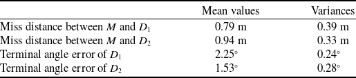
A table comparing mean values and variances of miss distances and terminal angle errors in a Monte-Carlo simulation where defenders have higher acceleration bounds. The table has four rows and three columns. The columns are labeled Mean values, Variances, and the row labels are Miss distance between M and D1, Miss distance between M and D2, Terminal angle error of D1, and Terminal angle error of D2. Row 1: Miss distance between M and D1, 0.79 m, 0.39 m. Row 2: Miss distance between M and D2, 0.94 m, 0.33 m. Row 3: Terminal angle error of D1, 2.25, 0.24. Row 4: Terminal angle error of D2, 1.53, 0.28.
Defenders have higher manoeuvring capabilities.

Figure 3. Long description
Panel A: A line graph depicts trajectories. The horizontal axis represents distance X in meters, ranging from 0 to 10000. The vertical axis represents distance Y in meters, ranging from -1000 to 1000. Four lines are plotted: Missile in blue, Target in orange, Defender1 in yellow, and Defender2 in purple. The trajectories show the paths taken by each entity. Panel B: A line graph depicts accelerations. The horizontal axis represents time in seconds, ranging from 0 to 12. The vertical axis represents acceleration in meters per second squared, ranging from -300 to 300. Four lines are plotted: Missile in blue, Target in orange, Defender1 in yellow, and Defender2 in purple. The accelerations show the changes in speed over time for each entity.
The accelerations of the vehicles are given in Figure 3(b). When the manoeuvring capabilities of the defenders are higher than that of the missile, the feasible region
 $\Omega$
will be an empty set. In this case, the acceleration of the missile reaches its maximum value in the endgame of the missile-defender engagements to try its best to evade defenders.
6.3 Monte-Carlo simulations
In this subsection, 500 Monte-Carlo simulations are given to verify the robustness of the design. The relative distances, relative velocities and line-of-sight angles are measured with Gaussian noise. The mean values are zero and the variances are 10 m, 1 m/s and 0.2
 $^\circ$
, respectively. Besides, a first-order linear dynamics with a time constant delay
 $\tau =0.2$
s is considered for each player. Statistics of the guidance performance for different cases are given in Tables 2 and 3. It is observed that the proposed approach is effective under various conditions. Adding the first-order time-delay elements for the players has little effect on guidance performance. In the real-world scenario, the noises and processing delays may reduce the theoretical safe region. Thus, in practice, larger
 $r_i$
than the exact values can be taken to calculate the safe region to guarantee the missile’s successful evasion.
7.0 Conclusions
In this paper, we solve the problem of designing guidance laws for agents in a TAD game involving qualitative and quantitative processes by proposing a hybrid differential game approach. The qualitative differential game theory is used to obtain the ranges which the guidance commands of the attacker take values in. The guidance laws of agents are then derived by solving the equilibrium solution of the quantitative differential game, with ranges obtained from the qualitative differential game treated as the feasible region for the attacker. The designed guidance laws are applied to the terminal guidance scenario. Simulation results verify the effectiveness of the design. When the number of defenders increases, the calculation amount may be large for the missile. The data processing capability of the missile needs to be further improved, which is worth noting for future work.
Competing interests
The authors declare none.