1. Introduction
‘Particle capture’ is the process by which particles in suspension contact a solid structure (‘collector’) and adhere to its surface. This process is of great ecological importance, as it controls the feeding and the reproduction of many aquatic organisms (Shimeta & Jumars Reference Shimeta and Jumars1991; Harvey, Bourget & Ingram Reference Harvey, Bourget and Ingram1995; Wildish & Kristmanson Reference Wildish and Kristmanson1997; Ackerman Reference Ackerman, Larkum, Orth and Duarte2006), as well as the ‘filtering’ of suspended particles by aquatic vegetation (Palmer et al. Reference Palmer, Nepf, Pettersson and Ackerman2004). Particle trajectories, and therefore particle capture, can be affected by the particle density ratio
 $$\begin{eqnarray}{\it\rho}^{+}=\frac{{\it\rho}_{p}}{{\it\rho}},\end{eqnarray}$$
where
 ${\it\rho}_{p}$
is the particle density and
 ${\it\rho}$
is the fluid density. Despite its relevance to ecological function, particle density effects have yet to be described in a parameter space relevant to aquatic environments.
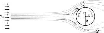
Steady-flow conceptualisation of the capture of finite-size particles influenced by inertia (
 ${\it\rho}^{+}>1$
). Particles are considered to be captured if they contact the collector. As the trajectories of particles influenced by inertia (indicated in black) do not coincide with the flow streamlines (indicated in grey), the capture efficiency (
 ${\it\eta}_{{\it\rho}^{+}>1}$
) differs from the perfect-tracer value (
 ${\it\eta}_{_{PT}}$
). The limiting streamlines – the outermost streamlines that allow capture and which define
 ${\it\eta}_{_{PT}}$
for perfect tracers of the same size (Espinosa-Gayosso et al.
Reference Espinosa-Gayosso, Ghisalberti, Ivey and Jones2012, Reference Espinosa-Gayosso, Ghisalberti, Ivey and Jones2013) – are indicated with dotted lines. The Cartesian coordinate system
 $(x,y,z)$
and the direction of the angular measures
 ${\it\alpha}$
and
 ${\it\theta}$
, used for presenting our results, are also indicated.

The process of particle capture is typically described for simplified geometries. Collectors (such as vegetation stems or the capturing filaments of suspension feeders) are modelled as cylinders, and particles (such as phytoplankton or suspended sediment) are modelled as spheres (figure 1). After a particle contacts the collector surface, it needs to be retained by an adhesive mechanism. Here, we consider perfect particle–collector adhesion, and all particles are assumed to be captured when they contact the cylinder surface. This is a reasonable assumption, as the periphyton layer that grows over aquatic vegetation surfaces (Borowitzka & Lethbridge Reference Borowitzka, Lethbridge, Shepherd, Larkum and McComb1989; Palmer et al. Reference Palmer, Nepf, Pettersson and Ackerman2004) and the mucous layer present on the collecting structures of suspension feeders (Shimeta & Koehl Reference Shimeta and Koehl1997) facilitate retention.
Traditionally, three different mechanisms of particle capture have been identified to occur on vertically oriented collectors (Hinds Reference Hinds1982): (i) ‘direct interception’, where the particle makes contact with the collector due to its finite size, (ii) ‘inertial impaction’, where the density influences its trajectory and promotes contact with the collector (figure 1), and (iii) ‘diffusional deposition’, where particle–collector contact is driven by random motions (such as Brownian motion). Following our previous work (Espinosa-Gayosso et al.
Reference Espinosa-Gayosso, Ghisalberti, Ivey and Jones2012, Reference Espinosa-Gayosso, Ghisalberti, Ivey and Jones2013), we study the capture of aquatic particles with diameters outside the colloidal range (i.e. we deal with the capture of plankton, larvae, pollen or sediment with diameters of
 $100~{\rm\mu}\text{m}$
or higher), a particle size range relevant to a variety of processes in aquatic systems (Espinosa-Gayosso et al.
Reference Espinosa-Gayosso, Ghisalberti, Ivey and Jones2012). In aquatic systems, diffusional deposition is important only for colloids and other micrometre-sized particles such as nanoplankton, bacteria and viruses (Shimeta Reference Shimeta1993), and is not considered here. For particles floating on the free surface, the additional mechanism of ‘capillary interception’ has been identified (Peruzzo et al.
Reference Peruzzo, Defina, Nepf and Stocker2013); but as our work focuses on the capture of particles in suspension, this mechanism is not considered here. We have recently obtained a complete description of the capture of perfect tracers (which are captured exclusively by the ‘direct interception’ mechanism) covering a range of particle sizes and flow conditions relevant to aquatic systems (Espinosa-Gayosso et al.
Reference Espinosa-Gayosso, Ghisalberti, Ivey and Jones2012, Reference Espinosa-Gayosso, Ghisalberti, Ivey and Jones2013). In the present study, we extend this work by considering the effects of the particle density ratio on the capture of aquatic-type particles.
For a cylindrical collector, the capture efficiency (
 ${\it\eta}$
) can be defined as the ratio of the number of particles captured (
 $N_{c}$
) to the number of particles whose centres would have passed through the space occupied by the collector were it not present in the flow (
 $N_{a}$
):
 $$\begin{eqnarray}{\it\eta}=\frac{N_{c}}{N_{a}}.\end{eqnarray}$$
Note that the definition of capture efficiency (1.2) allows efficiencies to be greater than 1 (see also Espinosa-Gayosso et al. Reference Espinosa-Gayosso, Ghisalberti, Ivey and Jones2012, Reference Espinosa-Gayosso, Ghisalberti, Ivey and Jones2013); this occurs when particles with centres outside the space defined by the collector diameter are intercepted due to their finite size. The maximum possible capture efficiency is thus
 $$\begin{eqnarray}{\it\eta}_{max}=1+r_{p},\end{eqnarray}$$
where
 $r_{p}$
is the particle size ratio, defined as
 $$\begin{eqnarray}r_{p}=\frac{D_{p}}{D}\equiv \frac{R_{p}}{R}.\end{eqnarray}$$
Here,
 $D_{p}$
and
 $R_{p}$
are the particle diameter and radius, and
 $D$
and
 $R$
are the collector diameter and radius, respectively. When only direct interception and inertial impaction are considered, the capture efficiency of finite-size particles depends upon three parameters:
 $$\begin{eqnarray}{\it\eta}={\it\eta}(r_{p},{\it\rho}^{+},\mathit{Re}),\end{eqnarray}$$
where
 $\mathit{Re}$
is the Reynolds number of the collector,
 $$\begin{eqnarray}\mathit{Re}=\frac{{\it\rho}U_{\infty }D}{{\it\mu}}.\end{eqnarray}$$
Here,
 $U_{\infty }$
is the uniform upstream fluid velocity and
 ${\it\mu}$
is the fluid viscosity.
The parameter typically chosen to represent the importance of particle inertia is the Stokes number (
 $\mathit{St}$
) (Friedlander Reference Friedlander2000). The definition of
 $\mathit{St}$
incorporates
 $r_{p}$
,
 ${\it\rho}^{+}$
and
 $\mathit{Re}$
:
 $$\begin{eqnarray}\mathit{St}=\frac{{\it\rho}_{p}D_{p}^{2}U_{\infty }}{9{\it\mu}D}=\frac{{\it\rho}^{+}r_{p}^{2}\mathit{Re}}{9}.\end{eqnarray}$$
Inertial impaction is typically thought to become dominant once
 $\mathit{St}$
exceeds a critical value. The existence of a critical Stokes number for aerosols (
 $\mathit{St}_{c,ae}$
) was first demonstrated by Taylor (Reference Taylor1940), who analysed aerosol particles (
 ${\it\rho}^{+}\gg 1$
) of negligible size (i.e. ideal ‘point’ particles with finite
 $\mathit{St}$
) approaching an object along the stagnation streamline. The critical Stokes number defines the minimum necessary
 $\mathit{St}$
for point particles (initially with the same velocity as the fluid) to reach the stagnation point. For inviscid flow and a cylindrical collector, Taylor (Reference Taylor1940) found that aerosol particles reached the collector in a finite time only if the Stokes number was above
 $\mathit{St}_{c,ae,inv}=1/8$
. For viscous flow, it has been recognised that the critical Stokes number (
 $\mathit{St}_{c,ae,{\it\nu}}$
) varies with Reynolds number (Langmuir Reference Langmuir1948; Davies & Peetz Reference Davies and Peetz1956; Matsufuji & Hasegawa Reference Matsufuji and Hasegawa1986; Lesnic, Elliott & Ingham Reference Lesnic, Elliott and Ingham1994; Phillips & Kaye Reference Phillips and Kaye1999) and accurate values for
 $\mathit{Re}\leqslant 1000$
have not yet been determined. There are no reported values of the critical Stokes number for particles with
 ${\it\rho}^{+}\sim O(1)$
, typical of aquatic systems.
There has been considerable analytical and experimental research into the effects of inertia on the capture of aerosols (see e.g. Davies & Peetz Reference Davies and Peetz1956; Fuchs Reference Fuchs1964; Fernandez de la Mora & Rosner Reference Fernandez de la Mora and Rosner1982; Fernandez de la Mora Reference Fernandez de la Mora1986; Flagan & Seinfeld Reference Flagan and Seinfeld1988; Wessel & Righi Reference Wessel and Righi1988; Friedlander Reference Friedlander2000; Haugen & Kragset Reference Haugen and Kragset2010). However, such studies are not applicable to aquatic systems, as they are characterised by one or more of the following conditions: (i) very high particle density ratios (
 ${\it\rho}^{+}\gg 1$
), (ii) a focus on a narrow range of flow conditions (usually inviscid or creeping flow fields, which can be described analytically), (iii) neglect of the finite particle size (
 $r_{p}\ll 1$
), and/or (iv) a focus on a range of
 $\mathit{St}$
where inertial impaction is entirely dominant. In aquatic systems, the particles of interest have a density similar to that of water (
 ${\it\rho}^{+}\sim O(1)$
and may even be positively buoyant (
 ${\it\rho}^{+}<1$
)), the flow conditions cover a wide range of
 $\mathit{Re}$
(
 $0<\mathit{Re}\lesssim 1000$
), particle sizes can be of the order of the collector diameter (
 $r_{p}\sim O(1)$
), and
 $\mathit{St}$
is in a range where particle density effects may be highly variable. The effects of the particle density ratio on particle capture have yet to be described in a parameter space relevant to aquatic systems.
As the particle density ratio
 ${\it\rho}^{+}\sim O(1)$
, the equations of motion for aquatic-type particles cannot be simplified to the equations typically used for aerosols (Babiano et al.
Reference Babiano, Cartwright, Piro and Provenzale2000) (see § 2.2). Indeed, for negatively buoyant particles (
 ${\it\rho}^{+}>1$
), the dynamics of aquatic-type particles are very different from those of aerosols over a wide range of flow conditions (Babiano et al.
Reference Babiano, Cartwright, Piro and Provenzale2000; Haller & Sapsis Reference Haller and Sapsis2008). For positively buoyant particles (
 ${\it\rho}^{+}<1$
), the differences are even more evident, as particles tend to drift towards the centre of curvature of the fluid pathlines in a centripetal, instead of centrifugal, manner (Maxey Reference Maxey1987). In this paper, we analyse how the particle density ratio modifies both the capture efficiency and the critical Stokes number in aquatic systems. We extend the classical approach of Taylor (Reference Taylor1940) to aquatic-type particles in inviscid and viscous flow to determine the dependence of the critical Stokes number on
 ${\it\rho}^{+}$
and
 $\mathit{Re}$
. For completeness, we also evaluate the critical Stokes number for aerosols when
 $\mathit{Re}\leqslant 1000$
. We use a numerical scheme to evaluate the effects of
 ${\it\rho}^{+}$
on the capture efficiency of aquatic-type particles by calculating their Lagrangian trajectories in mean flow fields (with time and axial averages obtained from direct numerical simulation (DNS)). Finally, we compare the capture efficiencies to those when perfect tracers are considered (i.e. pure direct interception (Espinosa-Gayosso et al.
Reference Espinosa-Gayosso, Ghisalberti, Ivey and Jones2012, Reference Espinosa-Gayosso, Ghisalberti, Ivey and Jones2013)) and discuss the reasons behind the differing behaviours.
2. Basic equations of motion and numerical methods
2.1. Equations of fluid motion
The governing equations are the continuity and Navier–Stokes equations for incompressible flow. Here they are non-dimensionalised with the uniform free-stream velocity
 $U_{\infty }$
as the velocity scale, and the radius of the collector
 $R$
as the length scale:
 $$\begin{eqnarray}\boldsymbol{{\rm\nabla}}\boldsymbol{\cdot }\boldsymbol{u}=0\end{eqnarray}$$
and
 $$\begin{eqnarray}\frac{\partial \boldsymbol{u}}{\partial t}+(\boldsymbol{{\rm\nabla}}\boldsymbol{u})\boldsymbol{u}=-\boldsymbol{{\rm\nabla}}p+\frac{2}{\mathit{Re}}{\rm\nabla}^{2}\boldsymbol{u},\end{eqnarray}$$
where
 $\boldsymbol{u}$
is the non-dimensional fluid velocity vector,
 $p$
is the non-dimensional pressure,
 $t$
is the non-dimensional time and
 $\mathit{Re}$
is the Reynolds number based on the diameter of the collector, as defined in (1.6).
Most results are presented in a non-dimensional cylindrical coordinate system
 $(r,{\it\theta},z)$
with the
 $z$
-axis coincident with the axis of the collector and
 ${\it\theta}$
is measured anticlockwise (figure 1). When relevant, results are presented in a non-dimensional Cartesian coordinate system
 $(x,y,z)$
with the origin and the
 $z$
-axis coincident with the cylindrical system.
2.2. Equations of particle motion
As in existing studies of particle capture influenced by inertia (Davies & Peetz Reference Davies and Peetz1956; Friedlander Reference Friedlander2000; Haugen & Kragset Reference Haugen and Kragset2010), we do not consider either particle motion, fluid motion or variation in collector geometry in the vertical direction, hence allowing a two-dimensional representation of this process. We also neglect the influence of the particles on the fluid motion, but we do consider the influence of the fluid flow on particle motion. Particle–particle interaction effects are neglected, as particle concentrations in aquatic systems are typically low. Our methodology also assumes that forces on the particles, such as lift induced by shear, ‘short-range’ (such as van der Waals or electrical double-layer) forces and hydrodynamic repulsion to contact, may be neglected to leading order. These assumptions have been tested in our previous work, where excellent agreement (within 6 %, on average) was obtained between existing experimental data and our capture efficiency estimates within the ranges
 $1\lesssim \mathit{Re}\lesssim 500$
and
 $0.01\lesssim r_{p}\lesssim 1.5$
(the reader is referred to figure 6 in Espinosa-Gayosso et al. (Reference Espinosa-Gayosso, Ghisalberti, Ivey and Jones2012) and figure 7 in Espinosa-Gayosso et al. (Reference Espinosa-Gayosso, Ghisalberti, Ivey and Jones2013)).
The Lagrangian equations for each particle (Maxey & Riley Reference Maxey and Riley1983; Auton, Hunt & Prudhomme Reference Auton, Hunt and Prudhomme1988; Babiano et al. Reference Babiano, Cartwright, Piro and Provenzale2000) can thus be written in non-dimensional form as:
 $$\begin{eqnarray}\displaystyle & \displaystyle \frac{\text{d}\boldsymbol{x}_{cp}}{\text{d}t}=\boldsymbol{v}_{cp}, & \displaystyle\end{eqnarray}$$
 $$\begin{eqnarray}\displaystyle & \displaystyle \frac{\text{d}\boldsymbol{v}_{cp}}{\text{d}t}=-\frac{f_{ns}}{\mathit{St}}(\boldsymbol{v}_{cp}-\boldsymbol{u}_{cp})+\frac{1}{{\it\rho}^{+}}\frac{\text{D}\boldsymbol{u}_{cp}}{\text{D}t}-\frac{1}{2{\it\rho}^{+}}\left(\frac{\text{d}\boldsymbol{v}_{cp}}{\text{d}t}-\frac{\text{D}\boldsymbol{u}_{cp}}{\text{D}t}\right), & \displaystyle\end{eqnarray}$$
 $\boldsymbol{x}_{cp}$
is the non-dimensional position vector of the centre of the particle,
 $\boldsymbol{v}_{cp}$
is the non-dimensional velocity of the particle and
 $\boldsymbol{u}_{cp}=\boldsymbol{u}(\boldsymbol{x}=\boldsymbol{x}_{cp}(t),t)$
is the fluid velocity at the position of the particle at any instant (consistent with the assumption that particles do not disturb the fluid); therefore
 $(\boldsymbol{v}_{cp}-\boldsymbol{u}_{cp})$
represents the velocity of the particle relative to the fluid. The three terms on the right of (2.4) describe the horizontal forces acting on the particle: the quasi-steady drag, the fluid-acceleration and the added-mass effect, respectively. We neglect the additional forces due to Faxén corrections and Basset–Boussinesq history, as our flow conditions (see § 2.3) are not highly variable in space or time and their contribution to the particle dynamics becomes of second order (Maxey Reference Maxey1987). The quasi-steady drag term accounts for non-creeping flow conditions by the use of a ‘non-Stokesian correction factor’ (Brandon & Aggarwal Reference Brandon and Aggarwal2001):
 $$\begin{eqnarray}f_{ns}=1+{\textstyle \frac{1}{6}}\mathit{Re}_{p}^{2/3},\end{eqnarray}$$
where
 $\mathit{Re}_{p}$
is the Reynolds number of the particle, based on the particle diameter and on the velocity of the particle relative to the fluid. The derivative
 $\text{D}\boldsymbol{u}_{cp}/\text{D}t$
is taken along the path of a fluid element,
 $$\begin{eqnarray}\frac{\text{D}\boldsymbol{u}_{cp}}{\text{D}t}=\frac{\partial \boldsymbol{u}_{cp}}{\partial t}+(\boldsymbol{{\rm\nabla}}\boldsymbol{u}_{cp})\boldsymbol{u}_{cp},\end{eqnarray}$$
while the derivative
 $\text{d}\boldsymbol{u}_{cp}/\text{d}t$
is taken along the trajectory of the particle,
 $$\begin{eqnarray}\frac{\text{d}\boldsymbol{u}_{cp}}{\text{d}t}=\frac{\partial \boldsymbol{u}_{cp}}{\partial t}+(\boldsymbol{{\rm\nabla}}\boldsymbol{u}_{cp})\boldsymbol{v}_{cp}.\end{eqnarray}$$
Therefore,
 $$\begin{eqnarray}\frac{\text{D}\boldsymbol{u}_{cp}}{\text{D}t}=\frac{\text{d}\boldsymbol{u}_{cp}}{\text{d}t}-(\boldsymbol{{\rm\nabla}}\boldsymbol{u}_{cp})(\boldsymbol{v}_{cp}-\boldsymbol{u}_{cp}).\end{eqnarray}$$
The particle momentum equation (2.4) can then be rewritten as
 $$\begin{eqnarray}\frac{\text{d}\boldsymbol{v}_{cp}}{\text{d}t}=-\left(\frac{2{\it\rho}^{+}}{2{\it\rho}^{+}+1}\right)\frac{f_{ns}}{\mathit{St}}(\boldsymbol{v}_{cp}-\boldsymbol{u}_{cp})+\frac{3}{2{\it\rho}^{+}+1}\frac{\text{D}\boldsymbol{u}_{cp}}{\text{D}t}.\end{eqnarray}$$
For aerosols (
 ${\it\rho}^{+}\gg 1$
), (2.9) can be further simplified to
 $$\begin{eqnarray}\frac{\text{d}\boldsymbol{v}_{cp}}{\text{d}t}=-\frac{f_{ns}}{\mathit{St}}(\boldsymbol{v}_{cp}-\boldsymbol{u}_{cp}).\end{eqnarray}$$
However, for aquatic systems with
 ${\it\rho}^{+}\sim O(1)$
, all the terms in (2.9) must be retained. Following Babiano et al. (Reference Babiano, Cartwright, Piro and Provenzale2000), we substitute (2.8) into (2.9) and rewrite it in terms of the velocity of the particle relative to the fluid:
 $$\begin{eqnarray}\displaystyle \frac{\text{d}}{\text{d}t}(\boldsymbol{v}_{cp}-\boldsymbol{u}_{cp}) & = & \displaystyle -\left(\frac{2{\it\rho}^{+}}{2{\it\rho}^{+}+1}\right)\frac{f_{ns}}{\mathit{St}}(\boldsymbol{v}_{cp}-\boldsymbol{u}_{cp})\nonumber\\ \displaystyle & & \displaystyle -~\frac{3}{2{\it\rho}^{+}+1}(\boldsymbol{{\rm\nabla}}\boldsymbol{u}_{cp})(\boldsymbol{v}_{cp}-\boldsymbol{u}_{cp})-\frac{2({\it\rho}^{+}-1)}{2{\it\rho}^{+}+1}\frac{\text{d}\boldsymbol{u}_{cp}}{\text{d}t}.\end{eqnarray}$$
This form of the momentum equation shows that neutrally buoyant particles (
 ${\it\rho}^{+}=1$
) and perfect tracers are not necessarily synonymous. For
 ${\it\rho}^{+}=1$
, the last term on the right-hand side of (2.11) disappears, but particles behave as perfect tracers only if the second term (the one containing the fluid velocity gradient) can also be neglected. In that case, after some initial difference between the particle and the fluid velocities, the relative particle velocity would decay exponentially with time (Babiano et al.
Reference Babiano, Cartwright, Piro and Provenzale2000) and particles would follow fluid paths exactly. But when either the fluid velocity gradient is large (as in zones close to stagnation points (Babiano et al.
Reference Babiano, Cartwright, Piro and Provenzale2000)) or when the particles are not perfectly neutrally buoyant, the last two terms on the right-hand side of (2.11) cannot be neglected, and particle dynamics differ from both those of perfect tracers and those of aerosols (2.10).
2.3. Mean fully developed flow conditions
To estimate particle trajectories, mean fully developed flow fields were first generated through two- and three-dimensional DNS, solving (2.1) and (2.2), as described in Espinosa-Gayosso et al. (Reference Espinosa-Gayosso, Ghisalberti, Ivey and Jones2012, Reference Espinosa-Gayosso, Ghisalberti, Ivey and Jones2013), using the open-source Navier–Stokes solver code OpenFOAM® v2.1.x (Weller et al.
Reference Weller, Tabor, Jasak and Fureby1998; OpenCFD 2012). The regimes of uniform flow past a cylinder are well documented (Zdravkovich Reference Zdravkovich1997). For
 $\mathit{Re}\lesssim 5$
the flow is steady and no recirculation bubble exists on the lee side. A steady recirculation bubble (formed by two symmetric recirculation vortices) exists on the lee side for
 $5\lesssim \mathit{Re}\lesssim 47$
. Above this value of
 $\mathit{Re}$
, the flow is unsteady and oscillatory conditions are forced by the growth and shedding of lee-side vortices. Oscillatory flow conditions induced by vortex shedding are not exclusive to the wake region, and are observed upstream of the cylinder (Espinosa-Gayosso et al.
Reference Espinosa-Gayosso, Ghisalberti, Ivey and Jones2013). When
 $\mathit{Re}>180$
, the flow in the wake becomes three-dimensional, and three-dimensional numerical solutions are needed to obtain accurate flow fields close to the leading face (Espinosa-Gayosso et al.
Reference Espinosa-Gayosso, Ghisalberti, Ivey and Jones2013). Calculation of particle capture estimates in unsteady flow fields is very computationally expensive. Therefore, in the range of unsteady flow conditions, DNS flow fields were first axially and time-averaged into mean flow fields before particle trajectories were calculated. For
 $\mathit{Re}>180$
, at least 50 oscillation cycles of fully developed flow were used for the temporal averaging, as the flow is no longer perfectly time-periodic when three-dimensional vortex shedding is present (Henderson Reference Henderson1997).
2.4. Numerical methods for estimating particle trajectories
Capture efficiencies and critical Stokes numbers were estimated with a Lagrangian approach by ‘seeding’ particles into the mean fully developed flow solutions described in § 2.3. Both the mean fluid velocity and mean velocity gradient fields were imported into MATLAB® release 2013b (MathWorks 2013), and the particle trajectories were calculated within the framework of this numerical tool. This methodology was previously tested (Espinosa-Gayosso et al.
Reference Espinosa-Gayosso, Ghisalberti, Ivey and Jones2013), and it was found that estimates of capture using mean flow fields differed by less than 1 % from estimates using the full unsteady flow field. Although the use of these mean flow fields does not precisely describe capture on the lee face of the collector, experimental (Palmer et al.
Reference Palmer, Nepf, Pettersson and Ackerman2004) and numerical (Haugen & Kragset Reference Haugen and Kragset2010) observations show that this is not a significant component of the total capture (
 ${<}5\,\%$
).
For the particle capture estimates, ‘clouds’ of particles of finite size were seeded into the computational domain upstream of the cylinder with an initial velocity equal to that of the local fluid at the particles’ initial positions (i.e.
 $\boldsymbol{v}_{cp}(t=0)=\boldsymbol{u}_{cp}$
). For critical Stokes number estimates, a single ‘point’ particle was seeded onto the stagnation streamline for each
 $\mathit{St}$
tested, and the
 $\mathit{St}$
was incremented by 0.0001 until a particle was able to reach the stagnation point. In the seeding zone, the fluid velocity was always within 0.01 % of the uniform flow condition, i.e.
 $(u,v,w)\approx (U_{\infty },0,0)$
. Particle trajectories were obtained by integrating (2.3) and (2.11) using an algorithm based on the explicit Runge–Kutta
 $(4,5)$
pair formula of Dormand & Prince (Reference Dormand and Prince1980). The fluid velocity and the velocity gradient at the centre of the particles (
 $\boldsymbol{u}_{cp}$
and
 $\boldsymbol{{\rm\nabla}}\boldsymbol{u}_{cp}$
) were obtained with a linear piecewise spatial interpolation of the mean DNS fields, which generates continuous fields at any position in the domain. The time step was always small enough to satisfy an absolute error tolerance of
 $1\times 10^{-6}$
. Particles were deemed to be captured when they touched the collector (i.e. when their centre came within one particle radius of the collector surface). Capture efficiency was estimated using (1.2) after all the non-captured particles had exited the domain.
3. The critical Stokes number
While the critical Stokes number is believed to indicate when inertia starts to affect the capture of small particles (Phillips & Kaye Reference Phillips and Kaye1999), inertial effects on particle trajectories have been observed even when
 $\mathit{St}$
is well below the critical value, owing to the compressibility of the particle phase (Robinson Reference Robinson1956; Michael Reference Michael1968; Fernandez de la Mora & Rosner Reference Fernandez de la Mora and Rosner1982; Fernandez de la Mora Reference Fernandez de la Mora1986). Strictly speaking, the critical Stokes number defines the minimum necessary
 $\mathit{St}$
for ideal ‘point’ particles (initially with the same velocity as the fluid) to reach the collector when moving along the stagnation streamline. Taylor (Reference Taylor1940) estimated the critical Stokes number for aerosol particles in inviscid flow (
 $\mathit{St}_{c,ae,inv}$
). In this section, we extend Taylor’s analysis of aerosols to viscous flow at
 $\mathit{Re}\leqslant 1000$
and to aquatic-type particles with
 ${\it\rho}^{+}\sim O(1)$
. We also evaluate the usage of the critical Stokes number in particle capture estimates.
3.1. The critical Stokes number for aerosols in inviscid flow
The non-dimensional velocity field of inviscid flow past a circular cylinder in cylindrical coordinates is (White Reference White2008)
 $$\begin{eqnarray}\left(u_{r},u_{{\it\theta}}\right)=\left(\cos {\it\theta}\left(1-\frac{1}{r^{2}}\right),-\text{sin}\,{\it\theta}\left(1+\frac{1}{r^{2}}\right)\right).\end{eqnarray}$$
Along the stagnation streamline (
 ${\it\theta}={\rm\pi}$
), the fluid moves in the negative radial direction only, i.e.
 $$\begin{eqnarray}\left(u_{r},u_{{\it\theta}}\right)_{{\it\theta}={\rm\pi}}=\left(-\!\left(1-\frac{1}{r^{2}}\right),0\right),\end{eqnarray}$$
and zero velocity is reached at the stagnation point (i.e. at the leading edge of the cylinder,
 $(r,{\it\theta})=(1,{\rm\pi})$
). The trajectory of an ideal ‘point’ aerosol particle (
 $r_{p}=0$
but with finite
 $\mathit{St}$
) approaching the collector along this stagnation streamline is obtained by substituting (2.3) and (3.2) into the momentum equation for aerosol particles (2.10) (note that, for point particles,
 $f_{ns}=1$
). The momentum equation can then be rewritten as
 $$\begin{eqnarray}\mathit{St}\frac{\text{d}^{2}r_{cp}}{\text{d}t^{2}}+\frac{\text{d}r_{cp}}{\text{d}t}+\left(1-\frac{1}{{r_{cp}}^{2}}\right)=0,\end{eqnarray}$$
where
 $r_{cp}$
denotes the radial position of the point particle. As this equation has no analytical solution, Taylor (Reference Taylor1940) further simplified (3.3) by approximating its non-homogeneous term as a linear function of distance from the stagnation point, resulting in the simplified equation of motion
 $$\begin{eqnarray}\mathit{St}\frac{\text{d}^{2}r_{cp}}{\text{d}t^{2}}+\frac{\text{d}r_{cp}}{\text{d}t}+2(r_{cp}-1)=0.\end{eqnarray}$$
The general solution of (3.4) is (Phillips & Kaye Reference Phillips and Kaye1999)
 $$\begin{eqnarray}r_{cp}(t)=\left\{\begin{array}{@{}ll@{}}\displaystyle \text{e}^{-t/2\mathit{St}}\left(A\,\text{e}^{(t\sqrt{1-8\mathit{St}})/2\mathit{St}}+B\,\text{e}^{-(t\sqrt{1-8\mathit{St}})/2\mathit{St}}\right)+1 & \text{for }\mathit{St}<1/8,\\ \displaystyle \text{e}^{-4t}(\hat{A}+\hat{B}t)+1 & \text{for }\mathit{St}=1/8,\\ \displaystyle \text{e}^{-t/2\mathit{St}}\left(\tilde{A}\,\cos \frac{t\sqrt{8\mathit{St }-1}}{2\mathit{St}}+\tilde{B}\,\sin \frac{t\sqrt{8\mathit{St }-1}}{2\mathit{St}}\right)+1 & \text{for }\mathit{St}>1/8,\end{array}\right.\end{eqnarray}$$
where the
 $A$
’s and
 $B$
’s are integration constants that depend on the initial position and initial velocity. The characteristic equation for the associated homogeneous equation of (3.4) is
 $$\begin{eqnarray}\mathit{St}\,m^{2}+m+2=0,\end{eqnarray}$$
and the changes in behaviour of the solution (3.5) depend on the values of the roots of (3.6). The characteristic discriminant
 $$\begin{eqnarray}{\it\Delta}=1-8\mathit{St},\end{eqnarray}$$
determines the values of the characteristic roots. The value of
 $\mathit{St}$
for which
 ${\it\Delta}=0$
(i.e. the critical Stokes number for aerosols in inviscid flow,
 $\mathit{St}_{c,ae,inv}=1/8$
) defines a transition in the behaviour of the solutions. Particles with
 $\mathit{St}\leqslant \mathit{St}_{c,ae,inv}$
have
 ${\it\Delta}\geqslant 0$
(i.e. real and negative characteristic roots) and never reach the stagnation point (
 $r=1$
) because
 $r_{cp}(t)>1$
at all times. Only those particles with
 $\mathit{St}>\mathit{St}_{c,ae,inv}$
have
 ${\it\Delta}<0$
(i.e. imaginary characteristic roots) and reach the stagnation point (i.e.
 $r_{cp}(t)\leqslant 1$
at some finite time) due to the oscillatory nature of the solution.
Numerical estimates of the critical Stokes number were obtained here by solving both the linearised equation (3.4) and the exact equation (3.3), using the methodology explained in § 2.4 but for analytical velocity fields. From the numerical solution of the linearised momentum equation (3.4) we obtained a critical Stokes number for aerosols in inviscid flow of
 $\mathit{St}_{c,ae,inv}^{num}=0.1251$
, in near-perfect agreement with linear inviscid theory. The numerical solution of the exact momentum equation (3.3) shows that the exact critical Stokes number is slightly higher,
 $\mathit{St}_{c,ae,inv}^{num,exact}=0.1260$
.
3.2. The critical Stokes number for aquatic-type particles in inviscid flow
When the added-mass and the fluid-force terms are retained in the particle momentum equation (2.11), the critical Stokes number differs from that of aerosols. The trajectory of a ‘point’ particle (
 $r_{p}=0$
but with finite
 $\mathit{St}$
and
 ${\it\rho}^{+}\sim O(1)$
) approaching the collector along the stagnation streamline is defined by substituting (2.3), (2.7) and (3.2) into (2.11), which can then be rewritten as
 $$\begin{eqnarray}\left(\frac{2{\it\rho}^{+}+1}{2{\it\rho}^{+}}\right)\mathit{St}\frac{\text{d}^{2}r_{cp}}{\text{d}t^{2}}+\frac{\text{d}r_{cp}}{\text{d}t}+\left(1-\frac{3\mathit{St}}{{\it\rho}^{+}{r_{cp}}^{3}}\right)\left(1-\frac{1}{{r_{cp}}^{2}}\right)=0.\end{eqnarray}$$
(Note that this equation simplifies to (3.3) for
 ${\it\rho}^{+}\gg 1$
.) Following the approach by Taylor (Reference Taylor1940), we approximate the non-homogeneous term as a linear function of distance from the stagnation point. The simplified equation of motion is
 $$\begin{eqnarray}\left(\frac{2{\it\rho}^{+}+1}{2{\it\rho}^{+}}\right)\mathit{St}\frac{\text{d}^{2}r_{cp}}{\text{d}t^{2}}+\frac{\text{d}r_{cp}}{\text{d}t}+2\left(1-\frac{3\mathit{St}}{{\it\rho}^{+}}\right)(r_{cp}-1)=0,\end{eqnarray}$$
with characteristic discriminant
 $$\begin{eqnarray}{\it\Delta}=1-8\mathit{St}\left(\frac{2{\it\rho}^{+}+1}{2{\it\rho}^{+}}\right)\left(1-\frac{3\mathit{St}}{{\it\rho}^{+}}\right).\end{eqnarray}$$
Particles with
 $\mathit{St}$
values for which
 ${\it\Delta}$
becomes negative will reach the stagnation point. The condition
 ${\it\Delta}=0$
defines the quadratic equation
 $$\begin{eqnarray}12(2{\it\rho}^{+}+1)\mathit{St}_{c,inv}^{2}-4{\it\rho}^{+}(2{\it\rho}^{+}+1)\mathit{St}_{c,inv}+{{\it\rho}^{+}}^{2}=0,\end{eqnarray}$$
whose smaller root determines the critical Stokes number in inviscid flow. This critical value (
 $\mathit{St}_{c,inv}$
) varies with
 ${\it\rho}^{+}$
, exceeding the aerosol critical value when
 $1<{\it\rho}^{+}\lesssim 1.5$
, and tends to the aerosol value (
 $\mathit{St}_{c,ae,inv}$
) from below as
 ${\it\rho}^{+}$
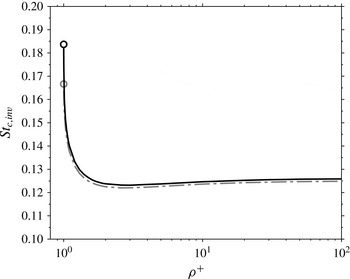
increases (figure 2). When
 ${\it\rho}^{+}=1$
the only root of (3.11) is
 $1/6$
, but particles do not reach the stagnation point for this value of the Stokes number (indicated by a circle in figure 2). Indeed, when
 ${\it\rho}^{+}\leqslant 1$
, the characteristic discriminant (3.10) is never negative and the solution of (3.9) never changes form. Therefore, ideal ‘point’ particles with a density equal to or less than that of the surrounding fluid will never reach the stagnation point (when starting with the same velocity as the fluid) and the critical Stokes number does not exist for
 ${\it\rho}^{+}\leqslant 1$
. The numerical solution of the exact momentum equation (3.8) shows that the exact values of the critical Stokes number are indeed slightly higher than the values obtained from the linearised theory.
The critical Stokes number for aquatic-type particles in inviscid flow (
 $\mathit{St}_{c,inv}$
) increases towards a finite value as
 ${\it\rho}^{+}\rightarrow 1$
, and towards the aerosol value (
 $\mathit{St}_{c,ae,inv}$
) as
 ${\it\rho}^{+}\rightarrow \infty$
. However,
 $\mathit{St}_{c,inv}$
does not exist for
 ${\it\rho}^{+}\leqslant 1$
(as indicated by the circles and the truncated lines). The dash-dotted line (— ⋅ —) is for
 $\mathit{St}_{c,inv}$
, the critical Stokes number obtained from the analysis of the linearised theory (3.11). The continuous line is for
 $\mathit{St}_{c,inv}^{num,exact}$
, the critical Stokes number obtained from the numerical solution of the exact momentum equation (3.8).

3.3. The critical Stokes number for aquatic-type particles in viscous flow
When a viscous flow is considered, the critical Stokes number (
 $\mathit{St}_{c,{\it\nu}}$
) differs from the inviscid value (
 $\mathit{St}_{c,inv}$
) due to differences in the radial velocity profile close to the stagnation point. Conservation of mass (2.1), together with the no-slip condition at the cylinder surface, imply that the radial velocity and its gradient in the radial direction are both zero at the collector surface, i.e.
 $$\begin{eqnarray}u_{r}=0\quad \text{and}\quad \frac{\partial u_{r}}{\partial r}=0\quad \text{at }r=1.\end{eqnarray}$$
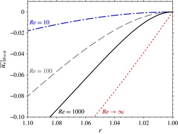
The fluid velocities close to the collector are thus more gradually varying than for inviscid flow (figure 3); hence, the drag force acting on the particles moving along the stagnation streamline is lower, in turn requiring additional mass (higher
 $\mathit{St}$
) in order for particles to acquire enough momentum to reach the collector (Davies & Peetz Reference Davies and Peetz1956; Phillips & Kaye Reference Phillips and Kaye1999). By considering two regions in the flow field: (i) a viscous boundary layer region close to the stagnation point and (ii) an inviscid flow region in the far field, Phillips & Kaye (Reference Phillips and Kaye1999) were able to estimate the critical Stokes number for aerosol particles in viscous flow (
 $\mathit{St}_{c,ae,{\it\nu}}$
) for
 $\mathit{Re}\geqslant 1000$
. Here, we estimate
 $\mathit{St}_{c,{\it\nu}}$
values in a range relevant to aquatic ecosystems (i.e.
 $\mathit{Re}\leqslant 1000$
and
 ${\it\rho}^{+}\sim O(1)$
), using the numerical methodology explained in § 2.4.
The mean radial velocity profile along the stagnation streamline (
 $\left.\overline{u_{r}}\right|_{{\it\theta}={\rm\pi}}$
) varies more gradually as the influence of viscosity increases. The lines represent inviscid flow (
 $\mathit{Re}\rightarrow \infty$
, from (3.2)) and DNS results at
 $\mathit{Re}=10,~100$
and 1000. The horizontal axis has been reversed to maintain the physical picture of the stagnation point (
 $r=1$
) on the right with
 $r$
increasing to the left.

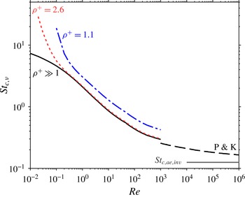
The critical Stokes number in viscous flow (
 $\mathit{St}_{c,{\it\nu}}$
) increases with decreasing
 $\mathit{Re}$
and
 ${\it\rho}^{+}$
. For aquatic-type particles, values of
 $\mathit{St}_{c,{\it\nu}}$
(obtained from DNS velocity fields) for two particle density ratios are shown: those for sediment-type particles (
 ${\it\rho}^{+}=2.6$
), and those for near-neutrally buoyant particles (
 ${\it\rho}^{+}=1.1$
). There is no curve for particles with
 ${\it\rho}^{+}\leqslant 1$
because
 $\mathit{St}_{c,{\it\nu}}$
does not exist in that case. The critical Stokes number for aerosols (
 $\mathit{St}_{c,ae,{\it\nu}}$
) is labelled as
 ${\it\rho}^{+}\gg 1$
. The results of the analytical approximation of Phillips & Kaye (Reference Phillips and Kaye1999) for aerosols is labelled as (P & K). The theoretical value for aerosols in inviscid flow (i.e. as
 $\mathit{Re}\rightarrow \infty$
),
 $\mathit{St}_{c,ae,inv}=1/8$
, is also indicated.

Equation (2.11) was solved for ideal ‘point’ particles (
 $r_{p}=0$
but with finite
 $\mathit{St}$
and
 ${\it\rho}^{+}$
) transported along the mean stagnation streamlines obtained from DNS for a range of Reynolds numbers and particle density ratios. For the mean flow conditions, (2.7) was used to simplify the last term in (2.11). For aerosols (
 ${\it\rho}^{+}\gg 1$
), the critical Stokes number increases as
 $\mathit{Re}$
decreases and, at low
 $\mathit{Re}$
, exceeds the inviscid value by up to two orders of magnitude (figure 4). Even at
 $\mathit{Re}=1000$
the value of
 $\mathit{St}_{c,{\it\nu}}$
for aerosols is more than double that of
 $\mathit{St}_{c,ae,inv}$
(in agreement with Phillips & Kaye Reference Phillips and Kaye1999). For aquatic-type particles with a density ratio similar to that of suspended sediment (
 ${\it\rho}^{+}=2.6$
) there is only a small increase of the critical Stokes number relative to aerosols, except when
 $\mathit{Re}$
is less than
 $0.3$
, for which the increase is significant. Finally, for near-neutrally buoyant particles (
 ${\it\rho}^{+}=1.1$
) the critical Stokes number is clearly greater than the aerosol value (by more than
 $50\,\%$
for all
 $\mathit{Re}$
). ‘Point’ particles with
 ${\it\rho}^{+}\leqslant 1$
do not reach the stagnation point for any
 $\mathit{St}$
and
 $\mathit{Re}$
.
4. Density-ratio effects on capture efficiency of aquatic-type particles
Here, we focus on the capture efficiency of finite-size aquatic-type particles (
 ${\it\rho}^{+}\sim O(1)$
) over ranges of
 $\mathit{Re}$
and
 $\mathit{St}$
(or
 $r_{p}$
) typical of aquatic systems. Lagrangian trajectories in mean flow fields (with time and axial averages obtained from direct numerical simulation (DNS), see § 2.3) were calculated using (2.11) for particles with three density ratios: (i) neutrally buoyant particles (
 ${\it\rho}^{+}=1$
), (ii) sediment-type particles (
 ${\it\rho}^{+}=2.6$
) and (iii) weakly buoyant particles (
 ${\it\rho}^{+}=0.9$
). Capture efficiencies were estimated using the procedure described in § 2.4 and the results were compared to the capture efficiencies of perfect tracers, i.e. when direct interception is the only capture mechanism (Espinosa-Gayosso et al.
Reference Espinosa-Gayosso, Ghisalberti, Ivey and Jones2012, Reference Espinosa-Gayosso, Ghisalberti, Ivey and Jones2013).
4.1. Neutrally buoyant particles
 $({\it\rho}^{+}=1)$

When particles are neutrally buoyant, their behaviour is very close to that of perfect tracers but, as discussed in § 2.2, deviations from fluid pathlines can appear in zones with large fluid velocity gradients (Babiano et al.
Reference Babiano, Cartwright, Piro and Provenzale2000). Nevertheless, for the
 $\mathit{Re}$
tested here, neutrally buoyant particles almost perfectly follow the mean streamlines and, as a consequence, the difference in particle capture efficiency for neutrally buoyant particles and perfect tracers is less than 0.1 % for
 $\mathit{Re}\leqslant 1000$
and
 $r_{p}\leqslant 0.5$
. That is, neutrally buoyant particles effectively behave as perfect tracers and only direct interception (Espinosa-Gayosso et al.
Reference Espinosa-Gayosso, Ghisalberti, Ivey and Jones2012, Reference Espinosa-Gayosso, Ghisalberti, Ivey and Jones2013) needs to be considered when evaluating their capture.
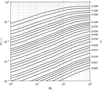
The capture efficiency diagram (figure 5) summarises our results for
 ${\it\rho}^{+}=1$
. This diagram covers particle sizes and Reynolds numbers in ranges relevant to aquatic systems and can be used for direct estimates of capture efficiency for given
 $\mathit{Re}$
and
 $r_{p}$
.
Capture efficiency diagram for neutrally buoyant particles of finite size (
 ${\it\eta}_{{\it\rho}^{+}=1}$
) as a function of the collector Reynolds number (
 $\mathit{Re}$
). Each line corresponds to a particular value of the particle size ratio (
 $r_{p}$
). (Values of
 $r_{p}$
are labelled on the right; unlabelled lines have values of
 $r_{p}$
at an equal interval between adjacent labelled values.) Differences from capture efficiency estimates of perfect tracers (Espinosa-Gayosso et al.
Reference Espinosa-Gayosso, Ghisalberti, Ivey and Jones2012, Reference Espinosa-Gayosso, Ghisalberti, Ivey and Jones2013) are negligible.

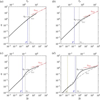
Capture efficiencies for sediment-type particles (
 ${\it\rho}^{+}=2.6$
) as a function of
 $\mathit{St}$
for (a)
 $\mathit{Re}=1$
, (b)
 $\mathit{Re}=10$
, (c)
 $\mathit{Re}=100$
and (d)
 $\mathit{Re}=1000$
. The capture efficiency (
 ${\it\eta}_{{\it\rho}^{+}=2.6}$
) is compared to that for perfect tracers of the same size (
 ${\it\eta}_{_{PT}}$
) and to the maximum possible capture efficiency (
 ${\it\eta}_{max}$
) (1.3). The first
 $\mathit{St}$
value with an increase of 10 % relative to
 ${\it\eta}_{_{PT}}$
is indicated with a
 $P$
(positive difference), and that with a decrease of 10 % is indicated with an
 $N$
(negative difference). The top axis indicates the corresponding particle size ratio (
 $r_{p}$
).

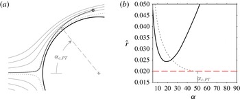
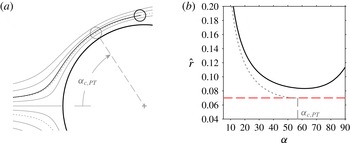
Graphical depiction of the centrifugal drift inducing a reduction in capture efficiency for sediment-type particles with weak inertial influence (
 ${\it\rho}^{+}=2.6$
,
 $\mathit{Re}=1000$
,
 $r_{p}=0.02$
,
 $\mathit{St}=0.11$
) relative to perfect tracers of the same size. (a) A particle with weak inertial influence (shown in black) released on the limiting streamline for perfect tracers of the same size (shown as a dotted curve) is able to escape capture (as indicated by its trajectory), thereby decreasing the capture efficiency relative to
 ${\it\eta}_{_{PT}}$
. A perfect tracer of the same size (shown in grey) would be captured at the maximum angle of capture (
 ${\it\alpha}_{c,PT}$
). (b) Distance from the centre of the particles in (a) to the collector surface (
 $\hat{r}=r_{cp}-1$
) as a function of the angle measured from the leading edge of the collector (
 ${\it\alpha}$
). The distance between the collector and the particle with weak inertial influence (continuous black line) is always larger than its radius (indicated with a horizontal dashed line) and capture never occurs. The distance from the collector to the perfect tracer (dotted line) is defined by the limiting streamline and meets the capture criteria at
 ${\it\alpha}_{c,PT}$
.

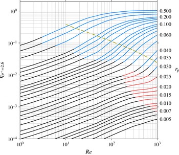
Capture efficiency of sediment-type particles (
 ${\it\eta}_{{\it\rho}^{+}=2.6}$
). (Nomenclature as in figure 5.) The region (top right) in which inertia augments capture efficiency by more than 10 % relative to the capture of perfect tracers (for the same
 $\mathit{Re}$
and
 $r_{p}$
) is shown in blue, and the region (centre right) in which inertia diminishes capture efficiency by more than 10 % is shown in red. The broken line indicates the particle size ratio (
 $r_{p}$
) that corresponds to the critical Stokes number (
 $\mathit{St}_{{\it\nu}}$
) at a given
 $\mathit{Re}$
(see also § 3.3).

4.2. Sediment-type particles
$({\it\rho}^{+}=2.6)$

Particles influenced by inertia do not follow fluid pathlines exactly (streamlines in steady flow), as shown in figure 1. The capture efficiency for particles influenced by inertia thus differs from the perfect-tracer value for the same
 $r_{p}$
and
 $\mathit{Re}$
. As expected, while increasing
 $\mathit{St}$
for a given
 $\mathit{Re}$
, inertial impaction of sediment-type particles promotes an increase in capture efficiency (
 ${\it\eta}_{{\it\rho}^{+}=2.6}$
) relative to perfect-tracer capture efficiency (
 ${\it\eta}_{_{PT}}$
) (figure 6); the vertical lines labelled as
 $P$
in this figure show the
 $\mathit{St}$
value at which the capture efficiency first increases by
 $10\,\%$
above the perfect-tracer value. This increase in capture efficiency occurs well before the critical Stokes number (
 $\mathit{St}_{c,{\it\nu}}$
, see § 3.3) is reached and, at the critical Stokes value, the increase in capture efficiency is considerably larger (15 % for
 $\mathit{Re}=1$
to 60 % for
 $\mathit{Re}=1000$
). Above the critical Stokes number, the increase in capture efficiency reaches a maximum. For example, for
 $\mathit{Re}=1000$
(figure 6
d), capture efficiency is 400 % greater than the value for perfect tracers at
 $\mathit{St}\approx 1$
. The critical Stokes number should not be considered as the starting point of inertial influence, but as an indicator of the region of inertial impaction dominance.
Inertia can also diminish capture efficiency under certain conditions (Fernandez de la Mora Reference Fernandez de la Mora1986). In our tests for
 ${\it\rho}^{+}=2.6$
and
 $\mathit{Re}\gtrsim 100$
, inertia reduces the capture efficiency relative to perfect tracers (at low
 $\mathit{St}$
) before an increase occurs (at higher
 $\mathit{St}$
). This reduction in capture efficiency is lower than 10 % for
 $\mathit{Re}=100$
, but for
 $\mathit{Re}=1000$
, the reduction is as large as 40 %; the vertical line labelled as
 $N$
in figure 6(d) shows the
 $\mathit{St}$
at which the capture efficiency first decreases by
 $10\,\%$
relative to the perfect-tracer value. This reduction in capture efficiency occurs as particles drift away from the collector due to centrifugal acceleration (Fernandez de la Mora Reference Fernandez de la Mora1986). The effect is illustrated in figure 7(a), which displays the trajectory of a particle, with weak inertial influence (
 $\mathit{St}=0.11$
and
 $r_{p}=0.02$
), released on the outermost streamline that allows capture of perfect tracers of this size (the limiting streamline for pure direct interception defined by Espinosa-Gayosso et al. (Reference Espinosa-Gayosso, Ghisalberti, Ivey and Jones2012, Reference Espinosa-Gayosso, Ghisalberti, Ivey and Jones2013)). A perfect tracer would follow the limiting streamline exactly and reach the collector at the maximum angle of capture on the leading face of the collector (
 ${\it\alpha}_{c,PT}$
) for perfect tracers of that size, but a particle influenced by inertia deviates from that trajectory. At first, close to the leading edge of the collector, the particle with weak inertial influence leaves the curving streamline, drifting centrifugally towards the collector. However, at the point of minimum distance from the collector, the particle has not yet been captured. Beyond this point, the particle drifts centrifugally away from the collector, allowing it to escape (figure 7
b). The net result is fewer particles reaching the collector, and a lower capture efficiency relative to that of perfect tracers. The reduction in capture efficiency appears well before any critical Stokes number estimated in § 3 (figure 6
d).
These results are summarised in the capture efficiency diagram (figure 8). The region in which inertia augments capture by more than 10 % relative to capture efficiency of perfect tracers (of the same
 $\mathit{Re}$
and
 $r_{p}$
) is shown in blue, and the region of more than 10 % reduction is shown in red. In the region of increased capture, the lines for specific
 $r_{p}$
are clearly steeper than for the neutrally buoyant (perfect tracer) case (figure 5), indicating a more rapid increase in capture efficiency with Reynolds number. A decrease in capture efficiency due to inertia occurs at large
 $\mathit{Re}$
and for small
 $r_{p}$
, as particles need to be small enough to not be intercepted before they reach the point of minimum distance from the collector (at which they start drifting away) (figure 7). Note that, for a given
 $\mathit{Re}$
, the regions of inertial augmentation or reduction occur for particles significantly smaller than the particle size corresponding to the critical Stokes number (
 $\mathit{St}_{{\it\nu}}$
) estimated in § 3.3.
Graphical depiction of the centripetal drift inducing a reduction in capture efficiency for weakly buoyant particles (
 ${\it\rho}^{+}=0.9$
,
 $\mathit{Re}=1000$
,
 $r_{p}=0.07$
,
 $\mathit{St}=0.76$
) relative to perfect tracers of the same size. (Nomenclature as in figure 7.) The weakly buoyant particle does not follow the limiting streamline and instead drifts towards the centre of curvature of the local flow. This allows the buoyant particle to escape, thereby decreasing the capture efficiency with respect to that of perfect tracers of the same size.

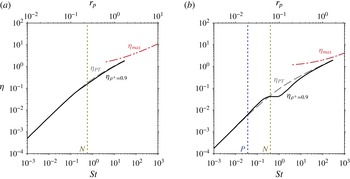
Capture efficiencies for weakly buoyant particles (
 ${\it\eta}_{{\it\rho}^{+}=0.9}$
) as a function of
 $\mathit{St}$
for (a)
 $\mathit{Re}=100$
and (b)
 $\mathit{Re}=1000$
. (Nomenclature as in figure 6.)

4.3. Weakly buoyant particles
$({\it\rho}^{+}=0.9)$

The difference in capture efficiency of buoyant particles (
 ${\it\rho}^{+}<1$
) relative to that of perfect tracers is due to the importance of the added-mass and fluid-acceleration terms in (2.4), which promote centripetal deviations of particle trajectories from fluid pathlines (Maxey Reference Maxey1987). Thus, when in a region of curved fluid pathlines (streamlines in steady flow), it is the drift towards the centre of curvature that modifies the capture efficiency relative to that of perfect tracers (figure 9); this is opposite to the ‘inertial impaction’ induced by the centrifugal drifting of particles denser than the fluid. In direct contrast to negatively buoyant particles, the deviation of weakly buoyant particles from fluid pathlines induces an increase in capture efficiency at lower
 $\mathit{St}$
and a more substantial decrease at higher
 $\mathit{St}$
; appreciable differences in capture efficiency are limited to
 $\mathit{Re}>100$
(figure 10). The differences relative to capture efficiency of perfect tracers increase with the Reynolds number, and for
 $\mathit{Re}=1000$
, capture efficiency reaches a maximum reduction of 60 %.
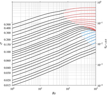
The capture efficiency diagram for weakly buoyant particles (
 ${\it\rho}^{+}=0.9$
) is shown in figure 11. Again, the zones of increase and decrease of capture efficiency, relative to that of perfect tracers, are coloured in blue and red, respectively. In contrast to negatively buoyant particles, an increase occurs for small particles with a decrease for larger particles. At large
 $\mathit{Re}$
, particles in the range
 $0.05\leqslant r_{p}\leqslant 0.1$
have a very similar value of capture efficiency, causing the curves to appear very close to each other. This can also be appreciated in the plot of capture efficiency as a function of
 $\mathit{St}$
for
 $\mathit{Re}=1000$
(figure 10
b), where
 ${\it\eta}_{{\it\rho}^{+}=0.9}$
has a plateau in the mentioned range of particle sizes.
Capture efficiency of weakly buoyant particles (
 ${\it\eta}_{{\it\rho}^{+}=0.9}$
). (Nomenclature as in figure 5.) The region (centre right) in which the centripetal drift of weakly buoyant particles augments capture efficiency by more than 10 % relative to the capture of perfect tracers (for the same
 $\mathit{Re}$
and
 $r_{p}$
) is shown in blue, and the region (top right) of a more than 10 % decrease relative to the capture of perfect tracers is shown in red.

5. Conclusions
For aquatic-type particles, we have used a Lagrangian analysis to estimate the influence of the particle density ratio on capture. We have shown that, for neutrally buoyant particles, the velocity gradients for
 $\mathit{Re}\leqslant 1000$
are not strong enough to induce significant deviations from a perfect-tracer trajectory, and their only mechanism of capture is direct interception.
When the particle density ratio is similar to that of sediment in water, inertia induces centrifugal deviations of particle trajectories from fluid pathlines and the effects are twofold: (i) inertia augments the capture efficiency relative to that of perfect tracers when the Stokes number is sufficiently large, and (ii) counter-intuitively, inertia can reduce capture efficiency for particles with weak inertial influence, i.e. at lower
 $\mathit{St}$
.
When particles are buoyant, the added-mass and fluid-acceleration terms induce a centripetal drift in particle trajectories. The centripetal drift can either augment or diminish particle capture relative to perfect-tracer capture but, unlike negatively buoyant particles, an increase occurs for smaller particles with a decrease for larger particles, i.e. higher
 $\mathit{St}$
.
For the first time, an analysis of the critical Stokes number for non-aerosol particles (aquatic-type particles) in viscous (
 $\mathit{St}_{c,{\it\nu}}$
) and inviscid flow (
 $\mathit{St}_{c,inv}$
) has been described. The critical Stokes number increases as the particle density approaches that of the surrounding fluid. When
 ${\it\rho}^{+}\leqslant 1$
, ideal ‘point’ particles never reach the stagnation point and the critical Stokes number does not exist. We also present, for the first time, the critical Stokes number for aerosols in viscous flow conditions (
 $\mathit{St}_{c,ae,{\it\nu}}$
) for
 $0.01\leqslant \mathit{Re}\leqslant 1000$
; in this range,
 $\mathit{St}_{c,ae,{\it\nu}}$
increases considerably with decreasing
 $\mathit{Re}$
.
Through the analysis of capture of dense aquatic-type particles of finite size (
 ${\it\rho}^{+}=2.6$
), we have shown that inertial effects are indeed significant at values of
 $\mathit{St}$
much lower than
 $\mathit{St}_{c,{\it\nu}}$
. The critical Stokes number should not be considered as the starting point of inertial influence, but as an indicator of the region of inertial impaction dominance. The influence of particle inertia on capture is maximised when
 $\mathit{St}>\mathit{St}_{c,{\it\nu}}$
and can result in as much as a fourfold increase in capture efficiency in aquatic systems.
Acknowledgements
A.E.-G. acknowledges the scholarships granted by CONACyT-Banco de México, the Australian Government (IPRS) and The University of Western Australia. Helpful comments from Professor J. Fernández de la Mora are gratefully acknowledged. This research was supported by the Australian Research Council Discovery Projects DP35603400 and DP150102638. This work was also supported by resources provided by the Pawsey Supercomputing Centre with funding from the Australian Government and the Government of Western Australia.