1 Introduction
The Distributional Hypothesis states that words with similar distributions have similar meanings. With varying degrees of explicitness, the hypothesis appeared in a number of different works in the 50’s, survived a period of relative obscurity, and has more recently been revived in the fields of cognitive psychology, in works like Miller and Charles (Reference Miller and Charles1991), and in computational linguistics, where it has been applied by a host of researchers with great success.
The following quotations capture the spirit of the Distributional Hypothesis:
The meaning of a word can be characterized by its distribution. (Nida Reference Nida1975, 167)
Strong Contextual Hypothesis: Two words are semantically similar to the extent that their contextual representations are similar. (Miller and Charles Reference Miller and Charles1991, 8)
To transform ideas like these into computationally practical systems, seminal works like Schütze (Reference Schütze1993); Dagan, Lee and Pereira (Reference Dagan, Lee and Pereira1997); Lee (Reference Lee1997); Lin (Reference Lin1998); and Dagan, Lee and Pereira (Reference Dagan, Lee and Pereira1999), explored various definitions of distribution and alternative similarity functions. What emerged was a family of vector space models of word meaning referred to as the ‘word as vector’ paradigm.
One of the less commonly explored consequences of the Distributional Hypothesis is that changes of meaning will be reflected in changes of word distribution. Thus, for example, the subtle shifts in word meaning observable in the ideologically charged writings of groups organized for collective political action could in principle be observed in shifts in the distributions of those words. Works like Gawron (Reference Gawron, Maienborn, von Heusinger and Portner2011) make it clear that groups organized for collective action do create a particular vocabulary expressive of their collective identity, and because that vocabulary sometimes involves general purpose vocabulary co-opted for group-specific senses (the word white as used by white militant groups), the property of interest is not the frequency of the word itself, but its usage pattern – for example, high co-occurrence frequencies of white modifying people, men, and identity, high frequencies of usage as a plural noun. Building up from there, we might hope to construct word hierarchies indicating word association patterns characteristic of the group, again relying on patterns of distribution among the words.
Interest in such an application places two important constraints on a word similarity system. First, it must be distributional; that is, it characterizes word meaning by patterns of usage. For example, any approach based on a domain-independent word graph such as WordNet is beside the point. Second, it cannot rely on the assumption that terabytes of data will be available. Groups organized for collective action often produce limited amounts of text; for this application, distributional systems must be able to squeeze the maximum amount of semantic information out of such limited datasets.
We are thus interested in the question of how similarity systems degrade when they move from modeling words for which we have representative data to modeling words for which the data is sparse, and when they fail altogether.
Consistent with our requirement that the models be usage-based, the word vector models in our study are all dependency-based models, models which build the word vector for a word w from statistics on all the modification relations w enters into in a parsed corpus. The counts for the dependency occurrences of the words man and liked in the sentence The tall man liked the small man are illustrated in Table 1. The word man enters into three parent relationships in this sentence (it is modified by three distinct word types) and two child relationships; its two tokens enter into two distinct modifying relations (signaled with a relation name that begins with − ).
Dependency feature counts extracted for man and liked based on the single sentence. The tall man liked the small man.

Thus, the appropriate statistic for measuring the amount of information we have on a word is its dependency count, the total number of parent/child relations the word enters into in the parsed corpus.
To illustrate the data sparsity issues involved, we will look at an example drawn from the 10,000 most frequent nouns in the British National Corpus, or BNC (Burnard Reference Burnard1995). If the word vectors are built using 50 million words, about half the BNC, the 10,000th most frequent noun (vagrant) has a dependency count of three. This is well below the point at which the word model can be used to make reliable similarity discriminations. However, consider dinghy, the noun at noun rank 6200Footnote 1, which has a dependency count of 215, distributed among 113 features. Of those 215 dependencies, many are semantically useless high count words like the (occurs 38 times) and a (occurs 22 times); 88 of the 113 features have count 1, and most of the semantically telling words can be found in this set, including words like inflating, maneuvering, fiberglass, and carry. This hapax list makes it very clear how low count events can still be informative despite inevitable noise: A word that shares a significant subset of the statistically interesting low count dependencies with our target word is probably related. Under such conditions, almost all events of interest are low count events. Ideally, we should still be able to make some useful discriminations with this amount of information.
An important subcase of the general problem is the issue of how to compare low frequency words with high frequency words. Suppose, we now want to measure the semantic similarity of boat, rank 682, 1057 non-zero features, with dinghy, rank 6200, 113 non-zero features. At the level of the vector representations we are using, these just look like events of very different dimensionality. The traditional recourse for comparing events of different scales is normalization. Normalization can be of two kinds. We can apply a transformation of the data that maps all events onto a single scale. Euclidean normalization does this. The risk of this strategy is the distortion of important relations in the data. Or we can perform a more costly normalization by pairs whenever we compare two events. Dice-family normalization, the kind used by the Dice Coefficient (Dice Reference Dice1945), is of this sort. We study both kinds of normalization. As we shall see, the normalized functions we are studying do not necessarily do sensible things when comparing words of very different frequency. For example, cosine is fairly ill-behaved. And a Dice-normalizing function like dice† (Curran Reference Curran2004) turns out to be a little better, but still not very good.
In this paper, we propose a novel approach to the problem of comparing representations of very different dimensionality; broadly speaking, we generalize Dice-family normalization with a weighting parameter α. This allows one to balance the differences in descriptive information between low and high dimensionality vectors. This approach necessarily results in an asymmetric similarity measure.
The idea of an asymmetric similarity measure seems to have originated with Tversky (Reference Tversky1977). Tversky’s main motivation for investigating asymmetry was to define a similarity model consistent with the results of a number of psychological experiments which demonstrated asymmetries in human similarity judgments. What Tversky proposes is actually a schema for a class of models, including as a special case a class of symmetric models. In Section 2, we demonstrate a previously unnoticed result, that Tversky models include all the Dice-family models as a special case, including important functions like Dice coefficient, Lin’s (Reference Lin1998) function, and the dice† function studied in Curran (Reference Curran2004). It follows from Tversky’s formulation that these functions have asymmetric versions that have previously been unstudied. We will show that the asymmetric versions of these functions improve on the performance of symmetric versions in a variety of tasks. We further show that the greatest improvement is always due to improvement in making comparisons between vectors of very different dimensionality, that is, in comparing less frequent words with frequent words.
With one exception, the set of tasks we will use to demonstrate the utility of the asymmetric Dice-family systems is drawn from a set of benchmarks tasks used in previous work on asymmetric similarity measures, including Lee (Reference Lee1999, Reference Lee2001), Weeds and Weir (Reference Weeds and Weir2005), and Jimenez, Becerra and Gelbukh (Reference Jimenez, Becerra and Gelbukh2012). This work has focused on showing that there is a class of tasks for which an asymmetric similarity measure is particularly well-suited. Here, we show the same improvements on some of the same tasks, but we focus on establishing a new result: One of the reasons asymmetry works when it works is that the best normalization strategy when computing the similarities of high dimensionality and low dimensionality representations is asymmetric. Thus, for example, in the nearest neighbor task which evaluates the quality of nearest neighbors found for testwords at a variety of frequencies, we show that asymmetric systems are best with very high and very low frequency testwords, when high–low dimensionality comparisons are most likely to occur.
The importance of asymmetry in facilitating high/low dimensionality comparisons is actually implicit in some of Tversky’s results (we discuss this in more detail in Section 2). Thus, the same kind of asymmetric system that works well on the benchmark asymmetric tasks in principle ought to work well at capturing human similarity judgments. We demonstrate this is the case by applying our Dice-family systems to several of the word-similarity datasets popular in the literature, including the Miller/Charles set (Miller and Charles Reference Miller and Charles1991), and show that asymmetric versions achieve dramatic improvements on their symmetric counterparts. To our knowledge, this is the first demonstration that an asymmetric word similarity measure models human judgments better than a symmetric measure (Tversky did not report on word similarity experiments, although this result would hardly have surprised him).Footnote 2
Accordingly, the rest of this paper divides into four parts. In Section 2, we introduce Tversky models and show their relationship with later work on word similarity. In Section 3, we describe the setup for four experiments demonstrating the effectiveness of the α-parameterized models, including human judgments. Our goal is twofold: first, to show there is a problem: Performance for normalized systems drops dramatically for rarer words; second, to demonstrate the benefits of α-parameterized systems are strongest for words at frequency extremes, very frequent and very infrequent words. In Section 4, we present our results, and finally, in Section 5, we discuss why α-parameterized systems perform as well as they do.
Our experiments will include symmetric and asymmetric Dice-family similarity measures and cosine (for the comparison with Euclidean normalization), as well as some unnormalized similarity measures. Thus, for example, we include dot product (or inner product) as one of our similarity measures, because it can be viewed as an unnormalized version of cosine. One of the most counterintuitive findings of this study is that unnormalized systems perform better with less frequent words than normalized systems. We show that α-parameterized systems and unnormalized systems lie on a continuum: The unnormalized systems can (for certain tasks) be thought of as maximally skewed systems in which similarity is simply measured by the unnormalized magnitude of shared information between the two words. The surprising result is that, in a number of applications, an unnormalized system may give the best performance with very rare words.
2 Asymmetry
Symmetry is a central assumption of most accounts of similarity, but it isn’t always a safe assumption, particularly when it comes to capturing the ways human judge similarity. Tversky (Reference Tversky1977) reviews the results of a number of different psychology experiments, including a number of his own, showing that human similarity judgments could be systematically asymmetric. Two examples of the kinds of judgments discussed are given here:
(1) An ellipse is more like a circle than a circle is [like] an ellipse.
(2) North Korea is more like China than China is [like] North Korea.
These examples illustrate one of his main findings: The variant is more similar to the prototype, in the sense of (Rosch Reference Rosch1975), than vice versa. One of the two models Tversky uses to try to account for asymmetry results is called a ratio model. The similarity calculation used by the ratio model is
 \begin{equation}
\dfrac{F(\text{A}\cap \text{B})}{F(\text{A}\cap \text{B}) +\alpha F(\text{A}\backslash \text{B}) + \beta F( \text{B}\backslash \text{A})}.
\end{equation}
Here, A and B represent feature sets for the objects being compared; the term in the numerator is the weight of the shared features, a measure of similarity, and the last two terms in the denominator are measures of dissimilarity: whenever α ≠ β, one set of dissimilarities gets a heavier weight, and we have asymmetry.
It’s instructive to consider a simplification of this model. If all feature values = 1 and α + β = 1, the model reduces to
 \begin{equation}
\text{sim}(\text{A},\text{B}) = \dfrac{\mid \!\text{A} \cap \text{B} \! \mid }{(1-\alpha )\!\mid \!\text{B}\! \mid + \; \alpha \! \mid \!\text{A}\! \mid }.
\end{equation}
Now, the similarity is just the cardinality of the set of shared features divided by a weighted sum of the cardinalities of A and B. The simplified form captures a basic prediction of the model. The potential for asymmetry will directly correlate with the difference in cardinality of the two sets. If the difference in cardinality (or total feature mass, in the unsimplified model) is great, then the similarity values of sim(A, B) and sim(B, A) can differ greatly for a given value of α. Conversely, if the two sets, or total feature mass, are the same size, then sim(A, B) and sim(B, A) are always the same and changing the value of α has no effect. This is illustrated in Figure 1. Tversky’s model predicts that significant asymmetry arises when there is a large difference in the aggregate masses of the two feature sets being compared. Thus, according to the model, that’s what must be happening in prototype/variant comparisons: there must be a large difference in the richness of the representations of the prototype and variant. Note that the same model would also tend to be asymmetric when comparing feature vectors with very different dimensionality. Thus, given a distributional representation of meaning, Tversky also predicts asymmetries should arise when comparing frequent words and less frequent words. In the remainder of this paper, we will be presenting various experiments to evaluate the performance of Tversky models across word ranks, bearing in mind that the cases where using Tverskyan models will make the most difference is when comparing words of very different ranks.
Tversky model: simplified.

Tversky notes the relationship of his ratio models to the similarity measure in Eisler and Ekman (Reference Eisler and Ekman1959), which proposes a similarity function equivalent to the earlier Dice Coefficient (Dice Reference Dice1945). Here, we develop the relationship of Tversky’s models to more recent similarity models generalizing Dice or using the same normalization strategy. To generalize the idea of feature matching from sets to real-valued features, we represent the total mass of a set of features shared by two vectors as the sum of the results of applying some operation si (for shared information) to each of the shared feature values. We refer to the sum of the shared information according to shared information operation si as σsi. This leads naturally to representing the dissimilarity of A and B as the difference between the information mass A shares with itself and the information mass it shares with B.Footnote 3
 \begin{equation}
\begin{array}{[}t]{c} \sigma _{\text{\sc si}}(\text{A},\text{B}) = \sum _{f \in \text{A}\cap \text{B}} \text{\sc si}(\text{A}[f],\text{B}[f])\\
\begin{array}{[}t]{|lll|} \hline \rule {0mm}{.15in}\text{F}_{\text{\sc si}}(\text{A}\cap \text{B}) & \Rightarrow & \sigma _{\text{\sc si}}(\text{A},\text{B})\\
\text{F}_{\text{\sc si}}(\text{A}/\text{B}) & \Rightarrow &\sigma _{\text{\sc si}}(\text{A},\text{A}) - \sigma _{\text{\sc si}}(\text{A},\text{B})\\
\hline \end{array}\\
\end{array}
\end{equation}
Taking all these assumptions together with the assumption that α + β = 1 leads us from Tversky’s original formulation to
 \begin{equation}
\text{{\sc T}}_{\alpha ,\text{\sc si}}(w_{1},w_{2}) = \frac{\sigma _{\text{\sc si}}(w_{1},w_{2})}{ (1 - \alpha )\cdot \sigma _{\text{\sc si}}(w_{1},w_{1}) + \alpha \cdot \sigma _{\text{\sc si}}(w_{2},w_{2})}.
\end{equation}
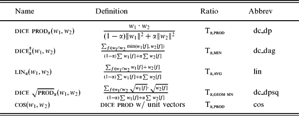
We will call equation (4) a generalized ratio model.Footnote 4Varying the si parameter, the shared information operation, yields different similarity functions, among them a number discussed in the literature. The variants used in this study are shown in Table 2.
Ratio models; the last column gives the abbreviation that will be used in figure legends.
Setting the si operation to be the product of two feature values gives us what we will call dice prod, popular in the data mining literature, for example (Strehl Reference Strehl2000, 55); setting it to be min gives us dice†, the function used in Curran (Reference Curran2004), and setting it to be the average of the two feature values gives us the function used in Lin (Reference Lin1998). Using geometric mean (the geometric mean of x and y is  $\sqrt{x \cdot y}$) yields a previously unstudied function we call dice
 $\sqrt{\text{{\sc prod}}}$. Cosine is just dice prod applied to unit-length vectors. Recognizing the conceptual importance of Dice’s original feature-set similarity function (Dice Reference Dice1945), we will refer to the normalization strategy employed in the denominator of (4) as Dice-family normalization.
In the experiments below, we will look at both symmetric and non-symmetric versions of all the functions in Table 2 (α = 0.5 and α ≠ 0.5) except cosine, for which asymmetry is not possible. As with the simplified model, when the aggregate feature masses of the vectors are all the same — in this case, all unit vectors — the ratio model doesn’t yield asymmetry. Thus, cosine is best seen as an instance of a different normalization strategy, Euclidean normalization, which is not α-parameterizable. We include cosine in our study to grade the performance of Euclidean normalization versus Tversky models.
Cosine has many mathematically appealing properties, including its scale- independence and its geometric interpretation, but from the present perspective it arises because Euclidean normalization is a natural scaling strategy: It provides a way of representing the information in small and large dimensionality vectors in comparable ways, and in that capacity Euclidean normalization can be applied beyond cosine. To explore this, and to better understand the limitations of Euclidean normalization, we will look at one other example: Euclidean normalization combined with geometric mean. We call the resulting similarity function dot$\sqrt{\text{{\sc prod}}}$euc. It is defined as follows:
 \begin{equation}
{\sc dot} \sqrt{\text{{\sc prod}}} {\sc euc}(w_{1},w_{2}) = \sum _{f \in w_{1}\cap w_{2} }\dfrac{\sqrt{w_1[f]}\cdot \sqrt{w_2[f]}}{\sqrt{\sum _f w_1[f]^2}\sqrt{\sum _f w_2[f]^2}}.
\end{equation}
Just as cosine is σprod — or dot product — performed on unit vectors, so dot$\sqrt{\text{{\sc prod}}}$euc is σgeom mn performed on unit vectors. dot$\sqrt{\text{{\sc prod}}}$euc is not mathematically pretty like cosine: It does not have a natural maximum or minimum, and self-similarity is not a maximum; because of this we will refer to it as a ‘pseudonormalized’ function.
There is an alternative normalization strategy which yields a truly normalized function for geometric mean, and that is L1 normalization, in which the normalization factor is ∑w[f] rather than  $\sqrt{\sum w[f]^2}$. When w = (w 1, w 2, . . ., wn), we write
 $\sqrt{\mathbf {w}}$ for
 $(\sqrt{w_1},\sqrt{w_2},\dots , \sqrt{w_n})$, ‖w‖2 for the L2 norm of w, and ‖w‖1 for the L1 norm. The
 $\sigma _{\sqrt{\sc prod}}$ operation applied to the L1 normalized version of w1 and w2 gives the cosine of
 $\sqrt{\mathbf {w_{1}}}$ and
 $\sqrt{\mathbf {w_{2}}}$:
 \begin{equation}
\begin{array}{[}t]{lllll} \cos (\sqrt{\mathbf {w_{1}}},\sqrt{\mathbf {w_{2}}}\,) & = & \frac{\sqrt{\mathbf {w_{1}}}}{\Vert {\sqrt{\mathbf {w_{1}}}}\Vert _{2}} \cdot \frac{\sqrt{\mathbf {w_{2}}}}{\Vert {\sqrt{\mathbf {w_{2}}}}\Vert _{2}} & = & \frac{\sqrt{\mathbf {w_{1}}}}{\sqrt{\Vert {\mathbf {w_{1}}}\Vert _{1}}} \cdot \frac{\sqrt{\mathbf {w_{2}}}}{\sqrt{\Vert {\mathbf {w_{2}}}\Vert _{1}}}\\
[.1in] & = & \sqrt{\frac{\mathbf {w_{1}}}{\Vert {\mathbf {w_{1}}}\Vert _{1}}} \cdot \sqrt{\frac{\mathbf {w_{2}}}{\Vert {\mathbf {w_{2}}}\Vert _{1}}} & = & \sigma _{\sqrt{\sc prod}}(\frac{\mathbf {w_{1}}}{\Vert {\mathbf {w_{1}}}\Vert _{1}},\: \frac{\mathbf {w_{2}}}{\Vert {\mathbf {w_{2}}}\Vert _{1}}). \end{array}
\end{equation}
Thus, we can think of L1-normalized  $\sigma _{\sqrt{\sc prod}}$ as taking the cosine of the data vectors in a transformed (compressed) space. The L1 system makes a very good similarity system with frequent words, but we will use the L2 system here because it is much better with infrequent words. In fact, it vastly outperforms cosine with infrequent words in the nearest neighbor task described below, a result which will help show the limitations of cosine in sparse word similarity applications.
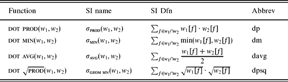
We will also include a set of unnormalized analogues of the functions in Table 2 in our study, to better understand how the performance of normalized functions changes across word ranks. As noted in the introduction, these functions, shown in Table 3, perform better with infrequent words than their normalized counterparts. In each case, the unnormalized function is simply the numerator of the definition of Tversky model function; that is, the sum of the shared information of the vector features.
The four unnormalized functions of this study; the last column gives the abbreviation that will be used in Figure legends.
Because of this, unnormalized systems are equivalent to α = 0 Tversky models on some tasks. In particular, for applications in which w 1 is held constant (which includes all the tasks described in Section 3, except the human judgment task), the similarity scores assigned by an α = 0 system are proportional to those chosen by its unnormalized counterpart. For example, when α = 0 for dice prod, we have
 \begin{equation}
\begin{array}{[}t]{lll} {\sc dice prod}_{\alpha =0}(w_{1},w_{2}) &=& \dfrac{w_{1} \cdot w_{2}}{\Vert {w_{1}}\Vert }\\
& \propto & w_{1} \cdot w_{2} = {\sc dot prod}(w_{1},w_{2}). \end{array}
\end{equation}
Since the denominator of the first line of (11) is independent of w 2, the relative similarities are determined by the numerator. Thus, for example, the α = 0 dice prod system will choose exactly the same nearest neighbors for w 1 as dot prod.
In sum, we will study ten basic similarity functions, four Tversky model functions, four unnormalized functions, and two Euclidean normalized functions, together with various asymmetric α-parameterized versions of the Tversky model functions.Footnote 5
Thus far, we’ve shown that asymmetric models can play a key role in accounting for human similarity judgments, basing our case purely on Tversky’s work, and we have shown that a class of Dice-family measures important in the literature are actually Tversky models, meaning that they have asymmetric versions. However, the advantages of asymmetry have actually been noted much more recently, for a different class of similarity functions, and motivated by very different concerns.
Motivated by the problem of measuring how well the distribution of one word w 1 captures the distribution of another w 2, Weeds and Weir (Reference Weeds and Weir2005) explore asymmetric models that compute similarity as a weighted combination of several variants of ‘precision’ and ‘recall’, scores that capture how well the features of w 1 predict those of w 2. W&W’s best-performing models, the additive precision/recall models, appear not to be Tversky models, since they compute separate sums for precision and recall from the f ∈ w 1∩w 2, one using w 1[f], and one using w 2[f]. However, one of their models actually is a Tverskyan ratio model. To see this, we divide (4) everywhere by σ(w 1, w 2):
 \begin{equation}
\text{{\sc T}}_{\text{{\sc si}}}(w_{1},w_{2}) = \dfrac{1}{\dfrac{\alpha \cdot \sigma (w_{1},w_{1})}{\sigma (w_{1},w_{2})} + \dfrac{(1-\alpha )\cdot \sigma (w_{2},w_{2})}{\sigma (w_{1},w_{2})}}.
\end{equation}
If the si is min, then the two terms in the denominator are the inverses of what W&W call difference-weighted precision and recall
 \begin{equation}
\begin{array}{[}t]{ll} \text{{\sc prec}}(w_1,w_2) = \dfrac{\sigma _{\text{{\sc min}}} (w_{1},w_{2})}{\sigma _{\text{{\sc min}}} (w_{1},w_{1})}\\
[11pt] \text{{\sc rec}}(w_1,w_2) = \dfrac{\sigma _{\text{{\sc min}}} (w_{1},w_{2})}{\sigma _{\text{{\sc min}}} (w_{2},w_{2})}. \end{array}
\end{equation}
So, for Tmin, (4) can be rewritten
 \begin{equation}
\dfrac{1}{\dfrac{\alpha }{\text{\sc prec} (w_{1},w_{2})} + \dfrac{1-\alpha }{\text{\sc rec} (w_{1},w_{2})}}.
\end{equation}
That is, Tmin (what we call dice†) is a weighted harmonic mean of W&W’s precision and recall, the so-called weighted F-measure (Manning and Schütze Reference Manning and Schütze1999). W&W discuss various ways of combining their precision and recall scores, including weighted harmonic mean, arithmetic mean, geometric mean, and weighted combinations of geometric and arithmetic mean, but they do not actually include a weighted harmonic mean in their evaluation.
Long before Weeds and Weir, (Lee Reference Lee1999) and (Lee Reference Lee2001) proposed an asymmetric similarity measure as well. Like Weeds and Weir, her perspective was to calculate the effectiveness of using one distribution as a proxy for the other, a fundamentally asymmetric problem.
For distributions q and r, Lee’s α-skew divergence takes the KL-divergence of a mixture of q and r from q, using the α parameter to define the proportions in the mixture
 \begin{equation}
\alpha \text{-skew}(w_{1},w_{2}) = \text{D}({w_{1}}{\alpha \cdot w_{2} + (1 - \alpha )\cdot w_{1}}),
\end{equation}
where D(‖) is KL-divergence, a measure of how much information is lost in using one distribution to predict another, and where the values in word vectors represent conditional probabilities:  $w[f] = \text{P}(f \mid w)$. Being fundamentally information theoretic, Lee’s model falls into a different class than either the W&W models or the Tverskyan models used here. However, we show in Section 4.4 that Lee’s model and the Tverskyan models perform comparably on a distribution prediction task, and in Section 5.3, we argue that they probably succeed for similar reasons.
3 Methods
We conducted four experiments to explore the performance of α-parameterized Tversky models.
(1) Correlation with human judgments for three wordsets:
(2) Nearest neighbor quality: nearest neighbors scored by PPR — a WordNet-based Personalized Pagerank system (Agirre et al. Reference Agirre, Alfonseca, Hall, Kravalova, Pasca and Soroa2009) — and ESA — a Wikipedia-concept based similarity system (Gabrilovich and Markovitch Reference Gabrilovich and Markovitch2009).
(3) Synonym detection: selecting a true synonym from a set of candidates, first used as an evaluation task with TOEFL questions (Landauer and Dumais Reference Landauer, Dumais, Kaplan and Burstein1994; Freitag, Blume, Byrnes, Chow, Kapadia, Rohwer, Wang Reference Freitag, Blume, Byrnes, Chow, Kapadia, Rohwer and Wang2005).
(4) Distribution prediction: Predicting noun distributions with nearest neighbors (Lee Reference Lee1999).
The last three tasks were all inspired by applications where improvements had previously been demonstrated for asymmetric similarity functions. We discuss each of these tasks in more detail in the following sections.
The systems were all dependency-based word vector models trained on a shared dataset on a single corpus, the BNC, parsed with the Malt Dependency parser (Nivre Reference Nivre2003). We parsed half the BNC, sections A– E and FA and F9, for a total of 52,432,977 words. This size corpus was sufficient to allow significant sparsity effects to crop up with the top 10,000 nouns, and to allow pairwise similarity comparisons against all nouns (not just the top 10,000) to be done for a large number of systems in reasonable computing time. The resulting dependency treebanks were used creating two dependency DBs, using basically the design in Lin (Reference Lin1998). Features were not pruned, except that negative value features were ignored in all the models. Feature pruning of course interacts with sparsity effects, which is what we are studying, but our preliminary goal in this paper is to look at sparsity effects with a very simple pruning model.
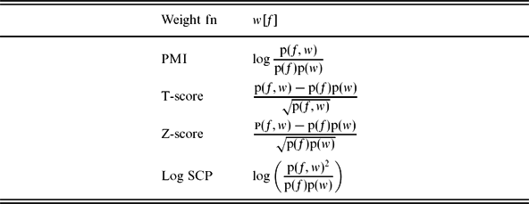
Weeds and Weir (Reference Weeds and Weir2005) use the term weight function for the function used to weight feature counts by their importance; for our feature function, we looked at four of the many possibilities in the literature. Three weight functions frequently used in similarity and collocation studies are Pointwise Mutual Information or PMI (Church and Hanks Reference Church and Hanks1990), T-score, and Z-score. Curran (Reference Curran2004) and Weeds and Weir (Reference Weeds and Weir2005) both report PMI to be among the most successful schemes, and Weeds and Weir report T-score to be the best, with Z-score and PMI among the strong contenders. We have included all three in this study.Footnote 6 We report results supporting this claim for the nearest neighbor experiment, as well as results for one other association measure which has achieved some success in collocation discovery, a log scale version of Symmetric Conditional Probability (Ferreira da Silva and Pereira Lopes Reference Ferreira da Silva and Pereira Lopes1999), which we will call Log SCP.Footnote 7 The formulae for all four weight functions are given in Table 4, where, P(f) denotes the probability of the feature f, P(w) the probability of a word, and P(f, w) their joint probability. The probability of any dependency type is estimated as its frequency divided by the number of dependency relations in the corpus. The frequency of a feature F is the number of tokens of the feature word serving the function associated with that feature. For example, the frequency of the man-subj feature is the number of times man has occurred as a subj (subject). The frequency of a word w is the total number of dependency relations it enters into in the corpus. We show that the improvements due to α-skewing can be observed with all four weight functions.
The four weight functions studied here.
3.1 Human judgments
For capturing human judgments, we will use rank-biased versions of ratio models, in which the α-weighted word is always the less frequent word.
 \begin{equation}
\begin{array}{[}t]{l@{\hspace{2.0pt}}l} \text{R}_{\alpha ,\text{{\sc si}}}(w_1,w_2) = \text{T}_{\alpha ,\text{{\sc si}}}(w_c,w_r)\\
\text{where } [w_{c}, w_{r} ]= \text{Order by rank}(\lbrace w_{1}, w_{2} \rbrace ). \end{array}
\end{equation}
The rank-biased similarity of w 1 and w 2 is just the ratio model similarity with the rarer word as the α-weighted argument.
The effect is shown Figure 2, in which wr is the rare word and wc is the common word: When α is high, what matters is the ratio of the shared information, σ(wc, wr), to the feature mass of the rare word (the smaller circle), and when it’s low it’s the ratio of the shared information to the feature mass of the common word (the larger circle). Borrowing the perspective of Weeds and Weir (Reference Weeds and Weir2005), we can think of an asymmetric measure of the similarity of two words as quantifying how well one word captures the distribution of the other. If we take the perspective of measuring how well wc captures the distribution of wr, then we might describe the rank-biased model by saying that high α emphasizes the recall score and low α emphasizes the precision score.
Effect of high α in rank-biased system.
The human judgement task is the only task for which we use rank-biased similarity. All three of the other tasks involve computing a set of similarities for some fixed noun we will call the target noun, which is always taken to be the first argument of Tσ, the word receiving weight 1 − α.
3.2 Nearest neighbor evaluation
This task is the simplest of the experiments. We use each system to find the nearest neighbors of the 10,000 most frequent nouns in the BNC corpus, and then evaluate the results. There is a solid body of previous work to fall back on for evaluating the quality of word similarity systems. Grefenstette (Reference Grefenstette1994) is a full-scale exploration of using existing online thesaurus resources to evaluate distributional word similarity methods; Lin (Reference Lin1998), McHale (Reference McHale1998), Curran (Reference Curran2004) reproduce and extend Grefenstette’s results considerably, and Weeds and Weir (Reference Weeds and Weir2005), Heylen et al. (Reference Heylen, Peirsman, Geeraerts and Speelman2008), and Bordag (Reference Bordag2008) offer alternatives with easier to apply WordNet-based evaluation tools.
In this task, we focus on evaluating nearest neighbors. This is like Heylen and one of the tasks in Weeds and Weir, but we differ in assigning a single evaluation score to a single nearest neighbor. Our primary goal is to study the degradation in performance as words get rarer, and to compare the rate at which the performance of different systems degrades. For this purpose, aggregating the nearest neighbor scores at 500-word intervals as we move from most frequent to least frequent in a set of 10,000 nouns gives very clear results. We experimented with two evaluation measures, very different in type, the personalized pagerank similarity measure of Agirre et al. (Reference Agirre, Alfonseca, Hall, Kravalova, Pasca and Soroa2009), a system the authors call PPR, and the concept-based Explicit Semantic Analysis, or ESA, system of Gabrilovich and Markovitch (Reference Gabrilovich and Markovitch2009).
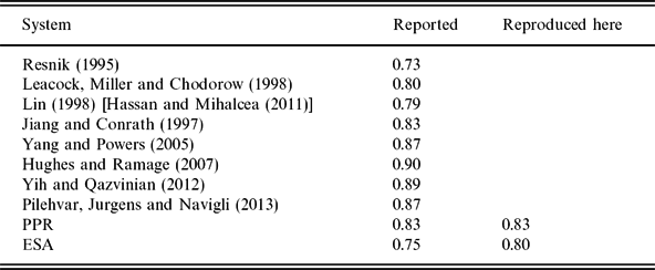
A few words motivating this choice. Table 5 summarizes the results for each of the Wordnet-based systems for Spearman correlations with human judgements of the Rubenstein–Goodenough/Miller–Charles wordset (Miller and Charles Reference Miller and Charles1991; Rubenstein and Goodenough Reference Rubenstein and Goodenough1965), a wordset used in a large number of word similarity studies. Reported numbers are taken from the summary in Agirre et al. (Reference Agirre, Alfonseca, Hall, Kravalova, Pasca and Soroa2009).Footnote 8 It can be seen that ESA and PPR exhibit at- or near- state of the art performance on MC/RG dataset, but performance on these benchmarks is not the only consideration. Two other factors were equally important.
Published system correlations with human judgments (RG/MC dataset). For the two systems used for evaluation here, we show the scores our re-implementations achieve.
First, both measures are defined in a way that makes them largely immune to word frequency effects. For this study, we need fairly robust measures which, as much as possible, retain the same level of resolution for rare and frequent words. PPR and ESA do this, PPR by being based on WordNet, ESA, by being built from the very large set of data available through Wikipedia.
As described in Agirre and Soroa (Reference Agirre and Soroa2009), the PPR measure is based on computing personalized pagerank vectors for each word in the WordNet graph, which requires resolving the following traditional pagerank equation:
 \begin{equation}
\text{Pr} = c\cdot \text{M{\bf Pr}} + (1 - c) \cdot {v}.
\end{equation}
Here, v is a vector of length N (the size of the graph), representing the probability of a surfer randomly teleporting to each node in the graph, M is a transition probability matrix for the entire graph, c is the probability of teleportation, (1 − c) the probability of following a link, and Pr is the pagerank vector for the graph. In the traditional pagerank measure, each node has probability  $\dfrac{1}{N}$ in v, but in personalized pagerank Haveliwala (Reference Haveliwala2003), the initial distribution of v has almost all the probability mass concentrated on one or more nodes ν, and on successive iterations that mass is transmitted outward along the links from ν. After some number of iterations (the authors cite 30), the computations of Pr are halted and the resulting Pr vector gives us a picture of what portions of the graph the nodes in ν is most richly connected to. Nodes that are similar to ν are connected to similar neighborhoods of the graph in similar ways. In the WordNet word similarity application, ν is the set of concepts associated with a word in WordNet, and the neighborhood is the set of concepts reachable via WordNet relations in the graph.
ESA describes each word as a weighted combination of all Wikipedia concepts. That is, it seeks to characterize a word’s meaning by the strength of its association with a set of known concepts. More specifically, a word in ESA is represented by a vector of length N, where N is the number of concepts in Wikipedia (roughly, each Wikipedia document is a concept), and each cell in the vector contains a TFIDF score for the word/concept pair. The similarity of two word vectors is computed by their cosine score.
Besides their excellent performance on the benchmarks, there were two other reasons for the appeal of ESA and PPR. First, both ESA and PPR work on words, whereas many of the path-based WordNet functions with state-of-the-art results work on concepts (for example, Lin and JCN) Our distributional word vectors represent word/part-of-speech pairs and thus correspond directly to PPR personalized pagerank vectors, which also represent word/part-of-speech pairs. A path-based similarity function such as the WordNet implementation of Lin and Jiang–Conrath however, can only score the similarity of two concept nodes. Accordingly, to evaluate nearest neighbor quality, we must either choose senses for the word pairs, or somehow average over all of them. The PPR pagerank vectors and ESA vectors, on the other hand, combine information about all the senses instantiated by the word form. This means no decision has to be made about which sense to use in the nearest neighbor calculation.
Second, ESA and PPR have been argued to measure different kinds of semantic distance. As noted in Agirre et al. (Reference Agirre, Alfonseca, Hall, Kravalova, Pasca and Soroa2009), the original RG/MC guidelines asked human judges to evaluate word pairs for semantic similarity, ignoring other semantic relationships that might obtain, such as strength of association. The guidelines for Wordsim made no such distinction. Thus, words like tiger and jaguar are semantically similar, denoting similar kinds of things in the world, but words like astronomer and star denote very different kinds of things, but are strongly associated. The Wordsim guidelines would seem to encourage annotators to value both pairs highly, and the RG/MC guidelines only to value tiger/jaguar highly. Both sets of guidelines yielded judgments with strong inter-annotator reliability, so both seem to be valid. Based on the results for the RG/MC and Wordsim wordsets performance discussed in Agirre et al. (Reference Agirre, Alfonseca, Hall, Kravalova, Pasca and Soroa2009), PPR targets semantic similarity, and performs less well at capturing semantic relatedness. Based on Gabrilovich and Markovitch (Reference Gabrilovich and Markovitch2009), ESA is very good at capturing semantic relatedness, performing very well on the full Wordsim dataset. A reasonable hypothesis is that semantic similarity is hard to capture with sparse data and that, in computing word similarity systems with less frequent words, we may be edging into territory where capturing semantic relatedness is a more realistic goal. However, it might also be the case that both kinds of similarity suffer with sparse data. Thus, it would be useful to try to measure both kinds of semantic connection, to see which is better preserved. As we shall see below, ESA and PPR largely agree in their estimates of system performance, so that discrimination of both semantic relatedness and semantic similarity seems to be impaired with less frequent words.
For the PPR-based evaluation, we used the precomputed wn30g word vectorsFootnote 9 and used dot product (which outperformed cosine) as our similarity measure, following Agirre et al. (Reference Agirre, Alfonseca, Hall, Kravalova, Pasca and Soroa2009). For ESA, we used the 2005 Wikipedia dump, Footnote 10 and Cagatay Calli’s well-documented implementation, with cosine as the similarity function. Footnote 11
To establish baselines we did the following: We paired each of the 10,000 test nouns with another of the 10,000 test nouns, chosen at random. We then scored the results with PPR and ESA. This yielded scores hovering around the same values at all word ranks, 0.00334 for PPR and around 0.0140 for ESA, indicating that despite the fact that cosine is used for both evaluations, ESA scores are in general about an order of magnitude higher than PPR scores. We will use these somewhat wavering lines as reference lines indicating random performance in the graphs below.
3.3 Synonym selection
The synonym selection task described in Freitag et al. (Reference Freitag, Blume, Byrnes, Chow, Kapadia, Rohwer and Wang2005) uses TOEFL-like test items: a test noun is paired with a synonym for one (possibly rare) sense, as defined by WordNet, and three randomly chosen distractor nouns.Footnote 12 The task is to pick out the true synonym. The task is more difficult than it may seem, because the test nouns are almost always ambiguous, and because the testset probes multiple senses of the same word, including some fairly obscure ones. For example, the noun test set (the one used in the experiments below) includes the following items using the WordNet lemma world as test item (the synonym is always the first word following the test item):

To facilitate comparison with previous work on this task, we also report results on the original TOEFL question set, basically identical in form. Its utility as evaluation tool for word similarity/clustering systems was pioneered in Landauer and Dumais (Reference Landauer, Dumais, Kaplan and Burstein1994), and results with this dataset have since been reported on in a number of studies, including (Turney et al. Reference Turney, Littman, Bigham and Shnayder2003) and Bullinaria and Levy (Reference Bullinaria and Levy2012). This testset differs from all the others in this study in that it is not limited to nouns.
3.4 Distribution prediction with nearest neighbors
In this task, a test item consists of a test verb, a test noun, and a distractor verb with roughly the same probability of occurrence as the test verb. The test noun has occurred as the direct object of the test verb in the BNC corpus, but not in the system training set, and the task is to try to choose between the test verb and the distractor based on the distributional facts of the test noun’s hundred nearest neighbors. Following the setup described in Lee (Reference Lee1999),Footnote 13 we set aside 20 per cent of the data as testset and select only test items where the noun and verb have not co-occurred in the training set. The decision procedure is Lee’s: Each neighbor votes for one of the verbs based on the weights assigned to the verb in its word vector; in ties both verbs receive one-half a vote. Eliminating test verbs that have co-occurred with the test nouns in the training data is particularly important for experimenting with less frequent nouns, because for such test items, the task actually becomes easier for less frequent test nouns. Consider the case in which the dependency set of a test noun contains the test verb and suppose the noun is a less frequent word. Since its nearest neighbors necessarily share dependency features with the test noun, they are actually more likely to also contain the verb in their dependency sets with a less frequent noun (with its smaller set of dependency features), and thus are more likely to correctly predict the co-occurrence. This is particularly true for this task, since to follow Lee’s original setup as closely as possible, we used pruned noun vectors that contained only instances of the -obj relation (verbs for which the noun had served the direct object function). We used five-ways cross-validation. For this evaluation, given the experiment model, we will include a comparison with the α-skew function that performed best in Lee (Reference Lee1999).
4 Results
4.1 Human judgments
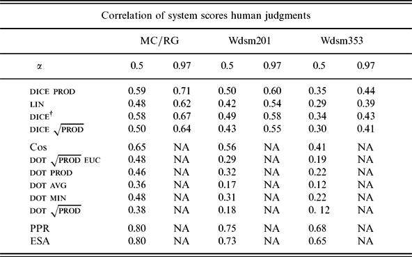
We turn to evaluating how well our ten core systems and the α-parameterized systems correlate with human similarity judgments. Table 6 shows the basic results from the Malt-parser based system for Spearman’s correlations with human judgments on the three word sets. The scores in the column labeled 0.97 are for highly skewed rank-biased systems (α = 0.97).Footnote 14 The scores to the left of those are scores for identical symmetric systems (α = 0.5). In each case, the rank-biased system shows a dramatic improvement over the corresponding symmetric system.
Similarity functions: Correlation with human similarity judgments for symmetric and asymmetric α systems.
For comparison, scores for the Euclidean systems cosine and dice$\sqrt{\text{{\sc prod}}}$euc are included below the first line, as well as the four unnormalized systems. As might be expected, the four unnormalized systems are consistently worse than the normalized systems. Cosine is the best of the ten symmetric distributional systems, but it can be seen that α-skewing makes two of the ratio model systems better than cosine.
The two scores below the second line are for our implementations of the systems we use for nearest neighbor evaluation, the Wordnet based PPR system and the ESA system. They are basically tied on the MC/RG dataset and perform at comparable high levels on the others.
4.2 Nearest neighbor task
We divide the results for the nearest neighbor task into two parts: performance with frequent words and performance across all word ranks. The takeaway point is that suitably parameterized α-systems are the best performers in both cases.
We first discuss performance with frequent words.
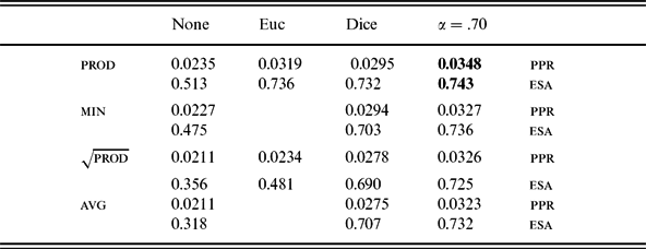
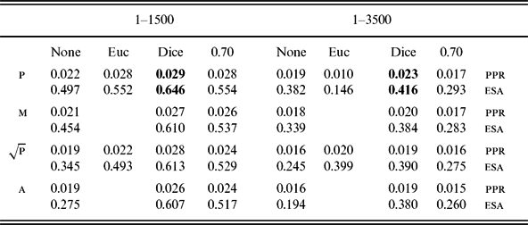
The results in Tables 7 and 8 give PPR and ESA numbers for all ten core systems combinations and for four α = 0.70 systems. Each cell contains the mean PPR and ESA scores for the nearest neighbor pairs discovered by a similarity system. Each row gives the result for one si for four systems: one with no normalization, one with Euclidean normalization, and two with Dice-family normalization. Thus, since cosine is dot product with Euclidean normalization, it is represented in the product row (labeled prod) in the Euclidean normalized column, with the raw dot product numbers to the left and the symmetric Dice-normalized version (which we called dice prod in Table 2) to the right. The symmetric Lin system is in the fourth row (the avgsi) in the Dice-normalization column. The last column is reserved for the α = 0.70 system score. Table 7 gives the results for noun ranks 1–500 and Table 8 gives aggregated results for two datasets, noun ranks 1–1500, and noun ranks 1–3,500. There are significant differences in both the numbers and relative strengths of different systems in the three datasets.
Ranks 1–500, core systems and α = 0.70 systems.
Ranks 1–1,500 versus 1–3,500, core systems and α = 0.70 systems.
The trends to notice are the following:
• Despite the differences in scale, ESA and PPR agree on the best and worst systems and there is significant agreement on the relative merits of the systems in all three datasets (e.g., the ESA and PPR scores on the 1–500 dataset have a Spearman’s correlation of 0.95, p < 0.001).
• Cosine is a very good system on 1–500 dataset (the best of the symmetric systems and even better than two of the α-systems, according to ESA), but it is the worst by far on the 1–3,500 dataset.
• Except for cosine, the normalized systems in the second, third, and fourth columns outperform the unnormalized systems in the first column on all three datasets, but the gap between them narrows considerably in the 1–3,500 dataset.
• The best systems on the 1–500 dataset are the α = 0.70 systems. Each of those systems outperforms its symmetric counterpart considerably (the score immediately to its left), on both the PPR and ESA evaluations. This is reversed on the 1–1,500 dataset, and on the 1–3,500 dataset, the α = 0.70 systems have gone from the best to nearly always the worst (except for cosine).
We turn to the main question of the paper: What system or systems perform best at low ranks? More precisely, we are interested in a system that degrades well: it performs well at high ranks (like cosine and the α = 0.70 systems) and remains robust at low ranks (unlike cosine and the α = 0.70 systems).
The plots in Figure 3 summarize the main results for the ten core symmetric systems across all 10,000 nouns. This graph shows the mean PPR scores (y axis) taken at 500 rank intervals (x-axis). We discuss the two panels in turn.
Top panel: PPR scores for top normalized systems across ranks: dot$\sqrt{\text{{\sc prod}}}$ with Euclidean normalization (dpsq euc), dice† (dc_dag), and dice prod (dc_dp). Unnormalized dot prod (dp) and random baseline added for comparison; Bottom panel: the four unnormalized systems dot prod (dp), dot min (dm), dot avg (davg), and dot$\sqrt{\text{{\sc prod}}}$ (dpsq), with Dice-normalized dice prod (dc_dp) and a random performance line for comparison.
Top panel: The top panel shows three of the best normalized core systems, dice prod (dc_dp), dice† (dc_dag), and dot$\sqrt{\text{{\sc prod}}}$ with Euclidean normalization (dpsq euc), with one unnormalized system, dot prod (dp), for comparison. The nearly horizontal line at about 0.003 shows random performance. Note that the best performer at low ranks is the unnormalized system, dot prod, which started out behind all the normalized systems in the 1–500 dataset, as shown in Table 7.
Bottom panel: The bottom panel shows that all four unnormalized systems from Table 3 perform better at low ranks than any of the normalized systems, excluding α-normalized systems. The representative normalized system shown is dice prod (dc_dp).Footnote 15
The bottom panel illustrates a key result for the symmetric systems: For the nearest neighbor task, normalization hurts with infrequent words. There are differences among the si’s as to how much it hurts and at what rank the effect manifests itself, but in the end it always hurts. For rarer words, an unnormalized system always outperforms its normalized counterpart, whether that normalization is Dice or Euclidean. The pattern is illustrated in Figure 4, which compares the systems using the  ${\sqrt{\sc prod}}$ and prod operations. With ${\sqrt{\sc prod}}$, Euclidean normalization performs better than Dice normalization; in both cases, however, the winner with infrequent words is the unnormalized system. Figure 5 shows that these results are replicated using ESA scores.
Top panel: PPR scores for the three prod systems, cosine (cos, Euclidean normalized) dice prod (dc_dp, Dice-normalized), and dot prod (dp, unnormalized), with the unnormalized system dot prod winning out with infrequent words; Bottom panel, PPR scores for the three ${\sqrt{\sc prod}}$ systems, dot$\sqrt{\text{{\sc prod}}}$euc (dqsq euc, Euclidean normalized) dice$\sqrt{\text{{\sc prod}}}$ (dc_dpsq), and dot$\sqrt{\text{{\sc prod}}}$ (dpsq, unnormalized), with the same result: the unnormalized system wins out with infrequent words.
ESA scores for same systems as in Figure 4. Top panel: the three prod systems, cosine (cos, Euclidean normalized), dice prod (dc_dp, Dice-normalized), and dot prod (dp, unnormalized), with the unnormalized system (dp) winning out with infrequent words. Bottom panel: the three ${\sqrt{\sc prod}}$ systems, dot$\sqrt{\text{{\sc prod}}}$euc (dpsq euc, Euclidean normalized), dice$\sqrt{\text{{\sc prod}}}$ (dc_dpsq, Dice-normalized), and dot$\sqrt{\text{{\sc prod}}}$ (dpsq, unnormalized), with the same result.
At the simplest level, what these results mean is that all the symmetric systems are very bad at noun rank 10,000 (the least frequent noun in the study). This is fairly clear because the unnormalized systems are bad with frequent nouns: they were the worst performers both and the 0–500 word set (Table 7). They continued to get worse from the 0–500 word set; they just did so at a slower rate than the normalized systems. At rank 10,000, they win by a large margin, because what the good systems do to be good has stopped working.
We have established that all the symmetric nearest neighbor systems studied here get worse with less frequent words, and that the Euclidean and Dice-normalization systems do so more rapidly, until they are actually worse then the unnormalized systems.
Turning now to the α-systems, we see that the steep decline of Dice-normalization systems can be arrested by tweaking the α parameter. The effect of varying α for dice prod and dice† is shown in Figure 6.
Sample of α systems for dice prod and dice†. Top panel: dice prod with various values of α. The symmetric system (elsewhere shown as dice prod, dc_dp) is α = 0.50. The α = 0.70 system is the best for frequent words (rank < 500), and the α = 0.04 system is the best with infrequent words. All systems are at or below random performance by rank 10,000. Bottom panel: The same pattern for dice†.
For both dice prod (top panel) and dice† (bottom panel), performance for infrequent words improves as α decreases. At the same time, performance for frequent words gets worse. The α = 0.04 systems are bad on 0–500 testset, but outperform symmetric dice prod (α = 0.50) and dice† (α = 0.50) from about rank 3500 on, creating a crossover of the performance curves. On the other hand, the pattern reverses when α > 0.5: The two α = 0.70 systems are far better than the α = 0.5 systems on the 1–500 testset, but the α = 0.70 systems crash far faster than the symmetric systems. Summarizing: Values of α above 0.5 yield very good frequent-word systems; values below 0.5 yield very good less frequent word systems.
The same trend shown for dice prod and dice† is replicated on the other two Dice-normalization systems: lin and dice$\sqrt{\text{{\sc prod}}}$. Values of α above 0.5 yield very good frequent word systems; values below 0.5 yield very good less frequent word systems. These are not shown here for reasons of space.
Figures 7 and 8 give the PPR scores across ranks for Dice family systems using T-score and Z-score, demonstrating that the improvements gained by α-skewing are not limited to the PMI weight function. Pairs of lines using the same Dice Family similarity functions are shown in each of the plots; for all four pairs with T-score, and for three of the four with Z-score, the α-skewed system is the one performing better with less frequent words; the exception is dice prod (dc_dp) in Figure 8, which is so bad with Z-score that performance for both the symmetric and skewed system falls below the random level by noun rank 1,000 (the 1,000th most frequent noun). Figure 9 plots the performance of the same four Dice-systems with the Log SCP weight function. The striking fact about Log SCP is not just that it mostly produces bad systems, but that for the one system that does perform well (dice†), the skewed system works best with all words, even the most common. We will propose an explanation for this in Section 5.
Symmetric (dashed lines) and α = 0.04 (solid lines) versions of T-score, showing an improvement for less common words for all four Dice-family functions.
Symmetric (dashed lines) and α = 0.04 (solid lines) versions of Z-score. Note that both dice prod systems with Z-score are very bad, scoring 0 on the 500–1000 dataset and below.
Symmetric and α = 0.04 versions of log SCP dice†, showing that for dice†, α = 0.04 is an improvement at ALL word ranks (no crossover). With the other functions, Log SCP’s performance is so bad, there are no results to report. dice prod on the upper right appears to be a case where the symmetric system crosses above the asymmetric system, but the random reference line shows this happens where performance is below random. The combination of Log SCP and Lin is so bad that performance is everywhere 0. This is worse than random because this system consistently chooses very rare nearest neighbors.
Figures 7–9 also demonstrate that PMI is the best of our weighting schemes across word ranks; in general, the T-score, Z-score, and Log SCP systems crash faster than the PMI systems. Hence, for the remaining evaluations, we focused on PMI.
4.3 Synonym selection
Figures 10 and 11 show the results of the synonym selection experiment with dice prod, the best performer. The y-axis shows accuracy at selecting the true synonym from among four candidates, and the x-axis, again, shows word rank. Figure 10 shows the results with at all frequencies. Two system lines are shown, the α = 0.04 system — marked with ‘+’ – versus the symmetric system (α = 0.5) — marked with diamonds. Clearly, the difficulty level of the various word sets does not correlate perfectly with decreasing frequency, since both performance lines zigzag up and down a fair amount, but what we see in Figure 10 is that with less frequent words the skewed α = 0.04 system outperforms the symmetric system quite consistently. Figure 11 zooms in on the most frequent words and shows the same mirroring asymmetry we saw on the nearest neighbor task: α-values greater than 0.5 help with more frequent words. The α = 0.70 and the α = 0.75 systems are better for the 1,000 most common words.
Synonym selection. The α = 0.50 and α = 0.04 systems using dice prod, from word ranks 0 through 16,000. With rare words, the α = 0.04 system consistently outperforms the α = 0.50 system.
Synonym selection focusing on word ranks 0 through 4,000. The α = 0.50 and α = 0.70 and α = 0.75 systems using dice prod. In the interval 0–1500, the two asymmetric systems outperform the α = 0.50 system.
Figure 12 gives the results on the very similar but much smaller TOEFL dataset. Distributed among the eighty items, the TOEFL testwords include a variety of parts-of-speech. Since we have been referring to noun ranks throughout (rank 1,000 means the 1000th most frequent noun), we have not tried separating the small testword set into smaller sets sorted by rank. The plot shows accuracy for the four Dice-family systems as a function of α-value. The best score, achieved with dice prod when α = 0.70, is 76.25 (with a 95 per cent confidence interval of 65.42–85.06). This equals the corpus-based result of Turney (Reference Turney2008), but falls below the 95 per cent confidence intervals of the hybrid system described in Turney et al. (Reference Turney, Littman, Bigham and Shnayder2003) [score: 97.5] and the corpus-based Singular Value Decomposition system in Bullinaria and Levy (Reference Bullinaria and Levy2012)[score: 100]. The takeaway points for our purposes are that α-skewing improves the performance of dice prod, dice$\sqrt{\text{{\sc prod}}}$, and lin, and that, with skewing, the smaller training set used here yields a system competitive with other distributionally trained systems.
TOEFL results: Four accuracy score lines are shown, one for each Dice-family function, dice prod (dc_dp), dice† (dc_dag), Lin (lin), and dice$\sqrt{\text{{\sc prod}}}$ (dc_dpsqrt), with the x-axis representing different values of α, decreasing from left to right. In general, accuracy decreases as α decreases, with one exception at one point for the dice† system, and the best score is achieved by a skewed system in which α = 0.70.
4.4 Distribution prediction with nearest neighbors
Figure 13 shows the results of the distribution prediction experiment. The task is to try to predict which of two verbs the test noun has actually co-occurred with, using information from nearest neighbor distributions. The y-axis shows prediction error rate, so lower is better. Error bars represent the highs and lows of the cross-validation runs. Once again, the best systems are heavily skewed, with very low values of α performing best with rarer words; but the novelty for this task is that a α-value greater than or equal to 0.5 is never the best system, even for the most frequent test nouns. The best system for the nouns ranked 0–1,000 is the heavily skewed α = 0.2 system. What the crossovers at rank 1,500 and rank 2,500 show is that as the target noun gets rarer, the optimal values of α get still lower, until from 3,500 on, 0 is the optimal value. So skewing always helps for this task, and the benefits increase at lower ranks.
Distribution prediction: All systems shown are dice prod systems, with error rates shown for words ranked 0–500, 500–1,500,1,500–2,500, 2,500–3,500, and 3,500–4,500. Performance lines are shown for eight different values of α, with error bars bracketing best and worst cross-validation runs. The best error rates are achieved by the system with the lowest α-value, α = 0.
Figure 14 compares the performance of the symmetric dice prod system and the α = 0dice prod to that of the α-skew function of Lee (Reference Lee1999) with the same data and experiment conditions. We see that the α-skew performance parallels the α = 0 performance across word ranks, but is slightly worse; however, both clearly outperform the symmetric system.
Comparison with Lee’s α-skew function. The dice prod α = 0 system outperforms α-skew consistently, and for all except the highest word ranks, both outperform the symmetric α = 0.50 system.
5 Discussion
5.1 Human judgments
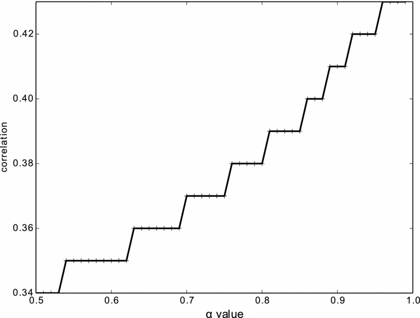
A preliminary worry with the human judgment results is that the improved correlation score is a kind of over-training effect, obtained by cherry-picking the particular α value that maximizes the correlation score. Figure 15 shows that in fact the scores improve monotonically: Gradually, increasing the α value from 0.5 to 0.97 gradually improves all the scores. At that point, some scores begin to turn downward.
Correlations with human scores monotonically increase with α.
Correlations with human judgments thus improve with increased skewing. The question is why. In understanding these correlation results, it helps to understand the particular way in which the results improve.
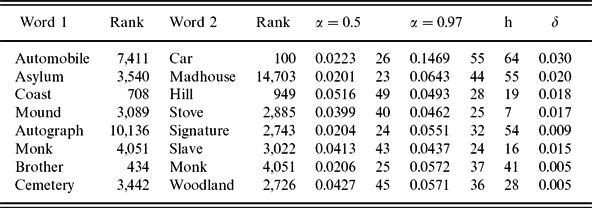
Recall that, with rank-biased systems, setting α to be greater than 0.5 weights the system in favor of recall of the rarer word’s features. In Table 9, we list the pairs whose reranking on the MC/RG dataset contributed most to the improvement of the α = 0.9 system over the default α = 0.5 system. Under each α-system, we list the pair score and rank among all the similarity scores for that system on that dataset, where 63 = most similar, and 0 = least similar. In the last two columns, we list the similarity rank according to human judgments (column labeled ‘h’), and an approximation of the amount of correlation improvement provided by that pair (δ):Footnote 16
Pairs contributing the most improvement in correlations with human judgments: α = 0.97, MC/RG word set.
Choosing α = 0.9 weights the similarity score toward recalling the features of the word with fewer modifiers and less information. Note the two items contributing the most improvement in the rank-biased system are pairs with a large difference in rank. For example, the proportion of automobile’s modifiers that are also modifiers of car contributes much more to the similarity score of car and automobile than the proportion of car’s modifiers that are also modifiers of automobile. Clearly, weighting the two proportions equally hurts in the α = 0.5 system, which greatly underestimates the similarity of the word pair. We hypothesize that rank bias toward the rarer word works because the more frequent words are more susceptible to ambiguities (car with cable, street, and railway, or trolley), or they may displace synonyms in collocations (car park, toy car); bias toward the rarer word works best when the frequent word has a salient ambiguity (as brother and signature do) or has metaphorical extensions or both (as is the case with asylum), because it allows modifiers particular to the other sense or extended uses to be forgiven. On the other hand, when the rarer word is ambiguous, results can be mixed. The word jaguar in the Wordsim set is a relatively infrequent word ambiguous between a cat-related sense and a car-related sense, and occurs in pairs that move in both directions:

Bias toward the rare word hurts in the second case, evidently because the car-related modifiers of jaguar penalize the similarity score, moving it in the wrong direction. Overall, rank bias works best with vectors of very different numbers of non-zero features.
5.2 Nearest neighbor task
Our results on the nearest neighbor task clearly establish two patterns: First, normalization correlates with a loss of performance with less frequent words. At the same time, normalization is responsible for clear gains in performance with the most frequent words; the best systems at ranks 1,500 and above, both in the nearest neighbor evaluation and in correlating with human judgments, were normalized systems, and most are Dice family normalized. Second, α-parameterization helps both with very frequent and very rare words: We saw that α-values below 0.5 dramatically improved nearest neighbor performance for Dice-family systems with rarer target words, while α-values above 0.5 help with very frequent words.
In fact, the improvements with α-skewed systems are monotonic; the optimal value for α starts well above 0.5 and drops as word rank increases. Thus, a symmetric system works best only with mid-frequency words. The following function of rank roughly captures the optimal value of α at word rank r.
 \begin{equation}
\alpha = e^{-(.0004r + .44)}.
\end{equation}
Figure 16 plots this function. We built a nearest neighbor system that varies alpha according to testword rank. That system is not the best at any rank but is the most consistent performer across all ranks:
A function which returns an approximately appropriate α-value for a rank r. The function shown is specific to the BNC corpus used here.
We address two questions in this section: Why should the performance of normalized systems decline so precipitously at low ranks, and why does α-normalization help?
We begin trying to answer this question by pointing to one statistic that strongly correlates with the decline of the normalized systems, as well as with the improvement registered in α-parameterized systems: average nearest neighbor rank (ANNR). For a given set of test nouns T and a given similarity function f, if $\text{NN}_{f}(w)$ is the nearest neighbor of w under f, then the ANNRf of T is
 \begin{equation}
\text{ANNR}_{f}(\text{T}) = \frac{1}{\left|\text{T}\right|} \sum _{w\in \text{T}} \text{Rank}(\text{NN}_{f}(w)).
\end{equation}
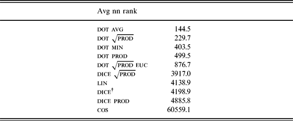
Table 10 gives the ANNR for all ten core systems for the critical 3000–3500 rank word set, ordering the systems from lowest average nearest neighbor rank to highest.
Average nn rank on the critical 3000–3500 test set.
We see that cosine, the worst system by far in this rank range, has an ANNR of over 60,000, an order of magnitude greater than the nearest competitor; in contrast, dice† has an ANNR of 4,199, and, at the other extreme, unnormalized dot prod has an ANNR of 500, meaning that, for most words in the test set, dot prod is choosing a nearest neighbor that is more frequent. Without normalization, long vectors have an intrinsic advantage; thus dot prod has a strong tendency to choose frequent words as nearest neighbors (low average rank). We might call this tendency length bias. Length bias is precisely the ailment that normalization is intended to cure; but Table 10 shows that the cure can be fatal. Cosine suffers from an egregious case of what we will call anti-length bias. The nearest neighbor set is heavily biased in favor of extremely rare words.
Figures 17 and 18 plot ANNR for the various systems evaluated on the nearest-neighbor task. The two plots demonstrate that ANNR slope is an excellent predictor of which systems will perform well with less frequent words. In all systems, ANNR rises for less frequent words, but those for which the rise is slowest are the best performers at low ranks. Figures 17 shows nine of the ten core systems; the system with the steepest slope, cosine, has been omitted for readability. The four systems crowded together near the x-axis are the four unnormalized systems, the best performers with rare words. The steepest slope shown belongs to dice prod, the second worst system with rarer words (after cosine), and the system steering a middle course between the normalized and unnormalized systems is dot$\sqrt{\text{{\sc prod}}}$euc, the pseudonormalized system which performed better than any normalized system with rare words. Figure 18 shows the ANNR slopes for the α systems, demonstrating that lowering α lowers ANNR slope. Again, the lower α was, the better the system performance on the nearest neighbor task with rarer words was.
Avg nn rank plotted versus target word rank for four Dice system, the pseudonormalized Euclidean system, and four unnormalized systems. As slope declines, performance at low ranks improves. Systems in decreasing slope order: dice prod (dc_dp), dice$\sqrt{\text{{\sc prod}}}$ (dc_dpsqrt), dice† (dc_dag), Lin (lin), dot$\sqrt{\text{{\sc prod}}}$ with Euclidean normalization (dpsq euc), dot min (dm), dot$\sqrt{\text{{\sc prod}}}$ (dpsq), dot avg (davg), and dot prod (dp).
Average nn rank for the dice prod α systems. The α = 0.50 system is labeled dc_dp in the legend. As α decreases, the slope of the system line decrease: The lowest sloping line belongs to the α = 0.07 system.
The highest slope in Figure 18 belongs to dice prod (dc_dp) and is roughly one. What an ANNR slope near one guarantees is that the system is rewarding neighbors close in rank to the target word. When there is a viable nearest neighbor in those ranks, this strategy pays off handsomely. The word jellyfish (found by several symmetric Dice systems) is a much better nearest neighbor for starfish than species (chosen by several unnormalized systems); but a close semantic relative whose related word whose rank is close to that of the target word may simply not exist, or if it does exist, the corpus may fail to contain a representative sample. In that case, the choices of a symmetric Dice-normalized system may look random. Consider brunt, chosen as the nearest neighbor of witness; brunt is the winner because the two words share a feature highly valued by PMI, − obj-bear, because of phrases like bear the brunt and bear witness. What the evaluation is showing is that such poor neighbor choices arise often for rare words. In exactly these cases, we see the less discriminating unnormalized systems making higher-valued choices.
Why does α-parameterization help? Repeating the definition of an α-parameterized Dice system from Equation (4):
 \begin{equation}
\text{{\sc T}}_{\alpha ,\text{\sc si}}(w_{1}, w_{2}) = \dfrac{\sigma (w_1,w_2)}{(1-\alpha )\cdot \sigma (w_{1},w_{1}) + \alpha \cdot \sigma (w_{2},w_{2})},
\end{equation}
we see that reducing α reduces the recall weight for w 2 (the testword), forgiving more information in w 2 not shared with w 1 (the target word), making it easier for long w 2 vectors to compete with short vectors in order to qualify as nearest neighbors. Thus, it is no surprise that ANNR goes down as α goes down: Lowering α in the nearest neighbor task does much the same thing as raising α did for the rank-biased α-systems in the task of correlating with human judgments. It allows words being compared to the word of interest — there the lower ranked word, here the target word — to be forgiven a few irrelevant modifiers. Note that raising α for frequent target words has the same effect: It forgives modifiers unshared by the larger vector. The generalization unifying the better-performing systems on both the correlation with human judgments and nearest neighbor tasks is this: In comparing vectors of very different sizes, bias in favor of capturing features of the shorter vector helps.
The risk of lowering α with infrequent words is length bias: Words with frequency equal to or lesser than that of the target word may now be undervalued; but according to the evaluation, this strategy is a win when the target word is less frequent. Mirroring this, when the target word is very frequent, the risk of raising α is anti-length bias, yet we saw that for very frequent target words, that strategy too is a win.
The results of this evaluation give us no real understanding of why rare words with little or no relation to the target word are overvalued when α = 0.5. We will leave this important question largely unanswered. We conclude this discussion with a few remarks that suggest a direction in which to search for an answer.
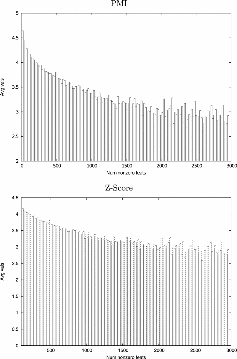
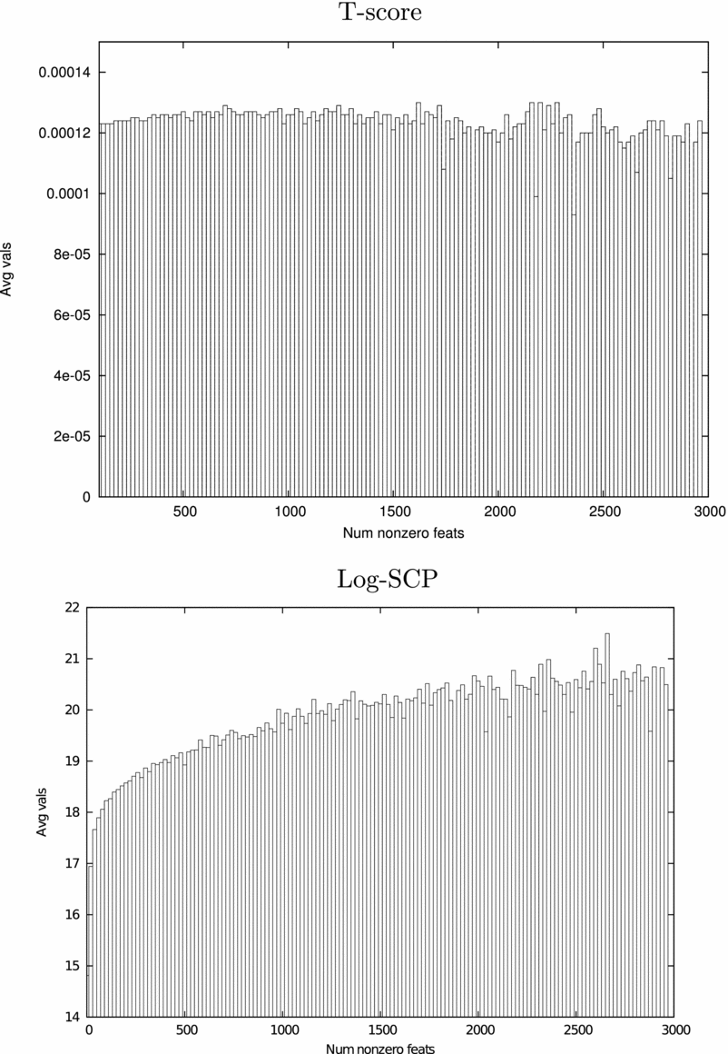
First, with PMI, the average feature value drops as vectors grow longer. The average feature value of a vector of course varies by weight function. The top panel of Figure 19 plots average feature value as a function of the number of non-zero-features for PMI, and, lest it be thought this is a special property of PMI, the bottom panel shows that it is also a property of Z-score. Figure 20 give the plots for the other two weight functions in our study, T-score and Log SCP. In Figure 19, we see average feature value dropping as the number of features increases. In Figure 20, in the case of T-score, average feature value remains roughly the same as the number of features increases, and in the case of log SCP, the weight rises. As noted in Section 4.2, the PMI, Z-score, and T-score perform reasonably with some functions, but log SCP seems to be non-competitive in this application. Generally speaking, feature weights are intended to be measures of statistical significance. Thus, it is perhaps not surprising that feature weights might rise with rarer words. Whether this is a ultimately desirable property for a weight function is unclear, but it is clear that assigning higher values for rarer words is a property of some important significance measures.Footnote 17
Average feature value as a function of vector length for PMI and Z-score. Average value falls for both.
Average feature value as a function of vector length for T-score and Log SCP. Average value remains roughly constant for T-score; and actually rises for Log SCP.
In Euclidean normalization, the values in large vectors are divided by a large number, and the values in small vectors values by a small number, so that the values of small vectors grow relative to those in large vectors. This distortion is worsened when the small vectors start with higher average values. The most extreme effects of this distortion are seen with cosine, where, with rarer target words, we see an extreme preference for rare nearest neighbors. Thus, the precipitous performance decline of cosine seen in Figure 4 can be traced to combining cosine’s inherent distortion with a weight measure (PMI) which worsens it. This analysis of cosine’s problems receives strong support from the fact that dot$\sqrt{\text{{\sc prod}}}$euc ameliorates the problem. While cosine is the worst performer with infrequent words, dot$\sqrt{\text{{\sc prod}}}$euc is one of the best. Taking the square roots of Euclidean normalized values reduces initial differences in average feature values.
On the other hand, with Dice-normalized systems, the effect of rising average feature values is to make longer vectors more competitive. Looking at (21), we see that for a given amount of shared information (σ(w 1, w 2)), a longer w 2 vector will, all things being equal, lose out to a shorter candidate, but if things are not equal, that is, if the shorter vector has higher average values, then the gap between them will shrink. That increasing the advantage of longer vectors helps is suggested by Figure 17, which shows us that better performing systems have higher ANNRs.
However, the results of our evaluation show that symmetric Dice-family systems do not increase the advantage of longer vectors enough; they still underperform with infrequent words, suggesting 0.5 is not a high enough α-value to overcome the advantage of shorter vectors with these target words. Figure 18 shows us that skewing to α < 0.5 further increases the advantage of longer vectors, and that correlates with improved nearest neighbor scores for these words.
If the average value of features actually grew with shorter vectors, even more skewing would be needed to advantage longer vectors. This is what seems to be happening with Log SCP. Figure 20 shows that, exceptionally, average value rises with vector size with Log SCP, and we saw in Figure 9 an α value of 0.04 achieved the best performance on the 1–500 dataset. This was the only case where an α-value less than 0.5 was helpful with frequent words.
5.3 Synonym detection and distribution prediction
At this point, the results across word ranks seen in the synonym detection and distribution prediction tasks should not be surprising.
The synonym detection task is really a smaller scale version of the nearest neighbor task. Instead of having its similarity computed for all the words in the lexicon, the target word has its similarity computed for a set of four testwords, with the largest scoring word chosen as the synonym. All the arguments about quality of nearest neighbor choice carry over to this task; and the results basically seem to mirror those in the nearest neighbor experiment.
The distribution prediction task is inherently asymmetric, which is why only skewed systems are competitive. The task is to measure how well nearest neighbors capture the distribution of the target word, and the converse relation is irrelevant. Thus, lowering α, which skews the system toward recall of the target word’s attributes was helpful. So, much was already apparent in the results reported by Lee for this task. What our results show that is novel is that the benefits of asymmetry increase (and the degree of asymmetry that is beneficial increases) as target nouns grow rarer. As with the nearest neighbor task, α = 0 was seen to obtain the best results with rarer words; with this task however, the α = 0 system became the best not just with rare words but even with words of medium frequency.
We saw in (11) that an α = 0 systems will choose the same nearest neighbors as its unnormalized counterpart. Since the similarity computation in our distribution prediction task is just the choice of the hundred nearest neighbors of the test noun, our dice prodα = 0 system would make the same distribution predictions as a dot prod system. Thus, we find that the best performer on this task, at least on words of mid to low frequency, is essentially an unnormalized system.
This is strongly reminiscent of Lee’s key result. Lee shows that an α-skew model depends only on the support of w 1 and w 2, which we have been notating w 1∩w 2. In particular, she notes that
 \begin{equation}
\alpha \text{-skew}(w_{1},w_{2}) = - \log \,(1 - \alpha ) +\\
\sum _{f \in w_{1} \cap w_{2}} w_{1}[f]\cdot (\begin{array}{[}t]{@{}l}\log w_{1}[f]\\
- \log \, (\alpha \cdot w_{2}[f] + (1 - \alpha ) w_{1}[f])\\
+ \log \,(1 - \alpha )).\end{array}
\end{equation}
Since dot prod, the unnormalized system that performed best here, also depends only on w 1∩w 2, we have confirmed evidence that the best distribution predictor should be a function of the support of w 1 and w 2.
Since both the dot prod function and α-skew increase monotonically with the mass of the support, we conjecture that the improvement achieved by our system has less to do with the variety of asymmetric model used than with the weight function determining the mass of the support. It may be that it pays to take into account the probabilities of the context words (P(f)) in the weight function, as PMI does (see Table 4), and as Lee’s conditional probabilities (P(f ∣ w)) do not.
6 Conclusion
We have achieved two significant results. We have shown that (a) classic normalization strategies applied to distributional systems fail to solve the problem of how to compare vectors of very different dimensionality; and (b) that a family of asymmetric Tversky-ratio models using Dice-style normalization provides a partial solution to this problem.
This work focuses on the problem of how to maximize the information available in sparse vectors, with the dataset fixed, and shows that, for some tasks, at least, α-parameterized functions make better use of that information than their symmetric counterparts. Having said that, it can be argued that all of the tasks used for evaluation here have a certain inherent asymmetry. Score comparisons in the nearest neighbor, synonymy, and distribution prediction tasks all involved maximizing the similarity of a set of candidates to a fixed testword. The success of the α-parameterized systems on the human judgment task, we argued, was because emphasizing the proportion of its features of the rare word shared helped zoom us in on the particular sense relevant to scoring high-similarity pairs. Arguably, that simulates something humans do, but computationally, rank-biased similarity is a rather special strategy not suitable for all similarity applications. Thus, our successes with asymmetric similarity are all very task specific. This, too, was a feature of the results Tversky was trying to model. Clearly, humans compute the similarity of China to Korea differently than they do the similarity of Korea to China. They interpret that particular task as asymmetric.
There are several directions in which to move in future work. First, the experiments here have focused entirely on distributional approaches based on syntactic models; it is important to explore whether similar sparsity effects plague context-window based models, and if they do (as we suspect they do), will asymmetry apply with equal success? Second, comparison of the approach here with that in Lee (Reference Lee1999) and Weeds and Weir (Reference Weeds and Weir2005) shows that different dimensions of asymmetry are explored in the different approaches. The approach pursued here introduces asymmetry into the normalization calculation. Lee and the additive models of Weeds and Weir introduce asymmetry into support computation (computing the aggregate weight of w 1∩w 2). These are orthogonal and potentially compatible strategies that could be explored together. Third, we have not investigated the interactions of feature pruning with sparsity, and the issue of how performance even with very rare words might be improved with the right kind of feature-pruning deserves a careful look. Finally, we need to better define the set of tasks for which asymmetry helps, or perhaps investigate the ways in which it can be better adapted to new tasks. Therefore, experimenting with new tasks like clustering is crucial.
Acknowledgments
This research was supported by NSF CDI grant #1028177. The authors are indebted to project members Ming Tsou, Dipak Gupta, Li An, Brian Spitzberg, Ick Hoi, Sarah Wandersee, Jennifer Smith, Ting-Hwan Lee, Amit Nagesh, Vickie Mellos, and Andrew McGladdery, as well as to the referees of an early draft, whose comments helped strengthen the arguments and better situate this work in the context of previous work.
Appendix A: Proof that Dice family functions are monotonic on Jaccard-family functions
We show that
 \begin{equation}
\sigma _{\text{\sc dice}}(w_1,w_2) > \sigma _{\text{\sc dice}}(w_3,w_4)
\end{equation}
if and only if
 \begin{equation}
\sigma _{\text{\sc jacc}}(w_1,w_2) > \sigma _{\text{\sc jacc}}(w_3,w_4).
\end{equation}
We first reformulate Dice and Jaccard in terms of ratios k 1 and k 2. For Dice, we have
 \begin{equation}
\begin{array}{[}t]{lll} \sigma _{\text{\sc dice}}(w_1,w_2) & =\dfrac{2 \cdot \sigma (w_{1},w_{2})}{\sigma (w_{1},w_{1}) + \sigma (w_{2},w_{2})}\\
&= \dfrac{2}{\dfrac{\sigma (w_{1},w_{1})}{\sigma (w_{1},w_{2})} + \dfrac{\sigma (w_{2},w_{2})}{\sigma (w_{1},w_{2})}}\\
& = \dfrac{2}{k_1 + k_2} & k_1 = \dfrac{\sigma (w_{1},w_{1})}{\sigma (w_{1},w_{2})}, k_2 = \dfrac{\sigma (w_{2},w_{2})}{\sigma (w_{1},w_{2})}. \end{array}
\end{equation}
Similarly, for Jaccard we have
 \begin{equation}
\sigma _{\text{\sc jacc}}(w_1,w_2) = \dfrac{\sigma (w_{1},w_{2})}{\sigma (w_{1},w_{1}) + \sigma (w_{2},w_{2}) - \sigma (w_{1},w_{2})} =\dfrac{1}{k_1 + k_2 -1}.
\end{equation}
So our reformulated proof goal is to show:
 \begin{equation}
\dfrac{2}{k_{1} + k_{2}} > \frac{2}{k_{3} + k_{4}} \;\text{ iff }\; \dfrac{1}{k_{1} + k_{2} -1 } > \frac{1}{k_{3} + k_{4} -1}.
\end{equation}
The following steps complete the proof from left to right and all steps are reversible. The steps rely on all the k being positive, which is guaranteed if all vector values are positive, a standard assumption.
 \begin{equation}
\begin{array}{[}t]{lll}
1. & \dfrac{2}{k_{1} + k_{2}} > \dfrac{2}{k_{3} + k_{4}}\\
2. & 2(k_{3} + k_{4}) > 2(k_{1} + k_{2})\\
3. & k_{3} + k_{4} > k_{1} + k_{2}\\
4. & k_{3} + k_{4} - 1> k_{1} + k_{2} - 1\\
5. & \dfrac{1}{k_{1} + k_{2} - 1} > \dfrac{1}{k_{3} + k_{4} - 1}\\
\end{array}
\end{equation}