1 Introduction
Sea ice, which forms in the cold, high-latitude regions of the Earth, such as the polar seas, covers 7%–10% of the world’s ocean surface. The mechanical breaking of larger ice masses like glaciers, icebergs or pack ice, due to wind, waves or collisions, often creates a type of sea ice that consists of small fragments of ice, called brash ice. These fragmented pieces, typically less than 2 metres in size, accumulate and float together on the ocean surface, forming a loose, chaotic mixture found in polar and subpolar regions [Reference Starosolszky52]. This natural formation of brash ice is common near the edges of ice fields or in coastal waters during the breakup season. Also, during the initial phase of sea ice formation (before it freezes solid), brash ice can be found as a slushy mixture of ice and snow. Unfortunately, brash ice affects offshore structures in the Polar Sea and makes shipping around ports more difficult and prone to navigational hazards. A detailed understanding of the sea ice–structure interaction is essential for the effective design and safe operation of polar vessels and offshore platforms. A recent and comprehensive review by Mohapatra and Guedes Soares [Reference Mohapatra and Guedes Soares45] further explains the advancements in nonlinear sea ice modelling and hydroelastic analysis, providing a critical survey of the theoretical and numerical methodologies used to examine complex ice–structure interactions. The study of submerged three-dimensional axisymmetric structures, such as cylinders, spheres and spheroids, remains under-explored in the context of brash ice. Understanding the hydrodynamic response of submerged structures in the presence of brash ice is particularly important for naval architects, especially when considering spheroidal shapes that more accurately represent the geometry of practical underwater vehicles and structures.
In the field of hydrodynamics, wave scattering by axisymmetric bodies of revolution has been the subject of extensive research for several decades. Although a substantial portion of the literature is dedicated to cylindrical geometries, analytical studies concerning spheroidal bodies remain relatively limited, with most focusing primarily on spherical cases. Notable contributions to the hydrodynamics of spherical bodies include the works of Gray [Reference Gray23], Wang [Reference Wang58], Wu and Eatock Taylor [Reference Wu and Eatock Taylor63, Reference Wu and Eatock Taylor65], and Linton [Reference Linton34], which provide valuable insights into wave interactions with submerged spheres. Moreover, some studies on submerged spheres even consider different boundary conditions [Reference Das and Mandal14, Reference Sturova54].
One of the core concepts in exploring the hydrodynamics of various axisymmetric submerged bodies is the use of different coordinate systems, such as the spherical coordinate system, the spheroidal coordinate system and the elliptical coordinate system. Miloh [Reference Miloh38] studied the forces and moments on a tri-axial ellipsoid using ellipsoidal harmonics and the method of image singularity. The interaction of waves with a horizontal elliptic disc submerged in a two-layer fluid was investigated by Das et al. [Reference Das, De and Mandal12], employing the eigenfunction-expansion matching method, formulated using Mathieu and modified Mathieu functions. The hydrodynamic response of a horizontal elliptic cylinder was studied by Gavrilov et al. [Reference Gavrilov, Ermanyuk and Sturova21], and Sturova [Reference Sturova53]. In addition to these, several researchers have examined complex structures, such as nearly circular rough plates, thin caps and elliptic discs employing appropriate geometric transformations, in accordance with the shape of the structures [Reference Das, De and Mandal10, Reference Das, De and Mandal11, Reference Hoque, Farina and Gayen29].
Recent advancements in wave–structure interaction have used three-dimensional (3D) Green’s functions to model complex fluid–structure interplays for various physical properties. Mohapatra and Guedes Soares [Reference Mohapatra and Guedes Soares43] used generalized expansion formulae for submerged flexible porous structures, incorporating orthogonal mode-coupling relations to investigate hydroelastic wave behaviour in channel environments. Additionally, Mohapatra and Guedes Soares [Reference Mohapatra and Guedes Soares44] developed a 3D hydroelastic model for horizontal flexible floating and submerged porous structures, deriving the dispersion relation through a Green’s function approach in both finite and infinite water depths. Their methodology employs 3D Fourier-type expansion formulae for velocity potentials and orthogonal mode-coupling relations to analyse interactions between porous plates.
Spheroids are a particularly important concept in hydrodynamics due to their applicability in modelling realistic marine structures subjected to wave-induced motions and forward-speed effects. Such configurations are relevant for analysing the hydrodynamic behaviour of autonomous underwater vehicles (AUVs), submarines, semisubmersible pontoons and buoyancy elements of SWATH vessels. Sir Thomas Havelock [Reference Havelock24–Reference Havelock26] laid the foundation in the field of spheroidal hydrodynamics, having determined the wave resistance of a submerged spheroid by modelling it as a distribution of sources and sinks or, equivalently, as a system of doublets. A semi-analytical method was proposed by Farell [Reference Farell18] to address the potential flow problem for a submerged prolate spheroid undergoing axial horizontal motion beneath a free surface. The author used the theory of infinitesimal waves to obtain the solution by expanding the sources distributed on the spheroid surface into a series of spheroidal harmonics. This approach was subsequently extended by Wu and Eatock Taylor [Reference Wu and Eatock Taylor62, Reference Wu and Eatock Taylor64] for the analysis of radiation and diffraction phenomena involving a prolate spheroid. Their method involves solving the classical Fredholm integral equation of the second kind for the unknown source distribution on the spheroid’s surface, employing series expansions in terms of Legendre functions. Thorne [Reference Thorne57] introduced the method of multipole expansions to analyse both spherical and cylindrical structures in water of finite and infinite depth. His formulations have been widely adopted in subsequent research to derive the diffraction and radiation components of the velocity potential surrounding submerged spheres. His formulations can also be effectively applied to axisymmetric bodies with geometries more complex than spheres, including prolate and oblate spheroids.
Miloh [Reference Miloh39] made a significant contribution to potential flow theory by deriving precise expressions for the ultimate image singularity systems linked to arbitrary exterior potential fields in prolate spheroids and triaxial ellipsoids. This research established a solid mathematical foundation for representing complex flow fields around ellipsoidal bodies, which served as the basis for analytical hydrodynamic modelling in such configurations. A key element of Miloh’s methodology was the application of Lagally’s theorem [Reference Lagally31] along with its subsequent generalizations [Reference Cummins9, Reference Landweber and Miloh32, Reference Landweber and Yih33], which he employed to evaluate the hydrodynamic forces and moments acting on ellipsoidal bodies submerged in unbounded inviscid fluid [Reference Miloh40]. Moreover, Miloh and Hauptman [Reference Miloh and Hauptman41] generalized this approach further to include spheroidal objects moving within confined fluid environments, such as canals or narrow basins, providing analytical perspectives on fluid–structure interactions in limited spaces. The validity of a theorem that Havelock [Reference Havelock27] had first hypothesized, but had not yet proven in the case of prolate spheroids, was proved by Miloh [Reference Miloh39], strengthening the theoretical foundation for further advances in spheroidal hydrodynamics. Chatjigeorgiou [Reference Chatjigeorgiou3] analysed the hydrodynamic diffraction by a submerged oblate spheroid by employing the method of multipole expansions, which was also used by the same author to investigate the diffraction problem of a submerged prolate spheroid. Later, Chatjigeorgiou and Miloh [Reference Chatjigeorgiou and Miloh5] proposed a generalized Thorne’s multipole expansion method based on Havelock’s theorem for solving the hydrodynamic problem of an axisymmetric and a nonaxisymmetric spheroid submerged below a free surface. The mathematical formulation is based on Havelock’s spheroid theorem, which represents exterior spheroidal harmonics through a defined system of singularities distributed along the major axis of the spheroid between its two foci. Subsequently, this method was employed to study the wave resistance and diffraction problem of a submerged spheroid [Reference Chatjigeorgiou and Miloh6] and the diffraction problem of a submerged spheroid advancing with forward speed [Reference Chatjigeorgiou and Miloh7]. Although there exists an ample amount of research in linear water waves theory, which studies different hydrodynamic aspects of submerged spheroids, only a few consider the presence of various natural occurrences, such as the surface tension, density stratification and the presence of ice at the free surface.
The present study focuses on the hydrodynamic response of a submerged prolate spheroid due to the surface wave on an ocean covered by brash ice. Our objective is to develop an analytical formulation for the associated wave diffraction problem. A few works model the brash ice mathematically. Peters [Reference Peters47] proposed a model of Brash ice that considers it as an infinitely thin mat composed of noninteracting particles for a fluid of infinite depth. The Steklov-type boundary condition on the free surface was used to take into account the presence of brash ice covering the water region. Weitz and Keller [Reference Weitz and Keller60] studied the reflection of water waves by a floating material of uniform surface density in water of finite depth. Although the effect of surface tension is often neglected in the linear theory of water waves, it has a significant impact on wave propagation. Wave interaction with bodies of various geometrical configurations has been analysed by researchers like Evans [Reference Evans16, Reference Evans17], Rhodes-Robinson [Reference Rhodes-Robinson48, Reference Rhodes-Robinson49], and Mandal and Basu [Reference Mandal and Basu35], when surface tension is present at the free surface. The boundary condition introduced by Peters [Reference Peters47] has the property that small amplitude surface waves cannot propagate for all frequencies when the brash ice is “too heavy”, although surface waves propagate for a sufficiently “light” layer of brash ice. However, Rhodes-Robinson [Reference Rhodes-Robinson50] demonstrated that the presence of surface tension, however little, is enough to ensure the propagation of capillary-gravity waves. Later, the same boundary condition was employed to study the generation of infinitesimal capillary-gravity waves in a motionless liquid with an inertial surface, due to a submerged wave source [Reference Rhodes-Robinson51]. Subsequently, Mandal and Kundu [Reference Mandal and Kundu36] investigated the wave generation problem due to different singularities in motionless water covered by an inertial surface, which was followed by their work where the authors additionally considered the effect of surface tension [Reference Mandal and Kundu37]. Recently, Kuznetsov and Motygin [Reference Kuznetsov and Motygin30] studied the two-dimensional modes of the coupled motion of a freely floating body and water covered by brash ice. Another important aspect is the presence of a continuous ice sheet at the ocean surface instead of broken ice. To mathematically model the ice-sheet, Fox and Squire [Reference Fox and Squire19] considered it as a thin elastic sheet and formulated the associated wave interaction problem. Afterwards, many notable studies were conducted on wave–structure interactions using the same ice-sheet model [Reference Das and Mandal13, Reference Das and Mandal15, Reference Fox and Squire20, Reference Sturova55, Reference Sturova56]. Furthermore, Mohapatra and Guedes Soares [Reference Mohapatra and Guedes Soares44] investigated the hydroelastic behaviour of a floating ice sheet near an impermeable wall under the influence of a following current. A significant recent advancement is provided by Biswas et al. [Reference Biswas, Das and De2], who employed the multipole expansion method, grounded in Havelock’s spheroid theorem, to analyse the linear hydrodynamic diffraction by both axisymmetric and nonaxisymmetric prolate spheroids fully submerged in infinite-depth water with surface tension effects at the free surface.
This research significantly contributes to the field of hydrodynamics by addressing the previously unexplored problem of water wave scattering by submerged spheroidal bodies in an ocean covered by brash ice. While existing literature has largely focused on cylindrical or spherical geometries, this study provides a more accurate representation of practical maritime structures, such as AUVs and submarines, by employing prolate spheroidal coordinates. The work is distinguished by its integration of physical parameters, specifically modelling brash ice as an inertial surface while simultaneously incorporating the effects of surface tension. The presence of surface tension ensures capillary-gravity wave propagation across all frequencies. The results provided by this study offer fresh analytical and numerical insights into how ice thickness and surface tension affect hydrodynamic loading, providing a specialized theoretical benchmark for designing modern underwater vehicles, such as AUVs and submarines, for polar operations.
Due to the natural occurrence of brash ice in many crucial regions, we present a study of wave diffraction by a prolate spheroid submerged in an ocean of infinite depth covered by brash ice. As detailed in Section 2, the brash ice has been modelled as a layer of uniform, noninteracting particles, as proposed by Rhodes-Robinson [Reference Rhodes-Robinson50], while additionally considering the effects of water surface tension. To take advantage of the symmetry of the object, a prolate spheroidal coordinate system has been used as described in Section 4. The Green’s function and its multipoles have been obtained in prolate spheroidal coordinates by using Havelock’s [Reference Havelock27] theorem to conveniently employ the method of image singularities, a methodology covered in Section 5. Finally, closed-form analytical and numerical solutions for both horizontal and vertical placements of the spheroid, along with their numerical validation, are presented in Sections 6 and 7. Conclusions are provided in Section 8.
2 Problem formulation
A rectangular Cartesian system (x, y, z) is chosen with the z axis being directed vertically downwards into an incompressible, inviscid fluid of infinite depth whose surface is entirely covered by a thin uniform layer of brash ice modelled as an inertial surface having area density
$\rho E$
 . Here,
$\rho $
 is the density of the fluid and E is the inertial surface parameter associated with a thin uniform layer of noninteracting fragmented pieces of brash ice, covering the ocean surface where
$E=(\rho {'}$
 /
$\rho )l$
 , where
$\rho {'}$
 is the density of the brash ice and l is the thickness of the brash ice modelled as an inertial surface. The plane
$z=0$
 represents the mean position of the surface covered by brash ice particles. A prolate spheroidal body is considered to be submerged at a distance d below the mean position of the inertial surface. The fluid motion is assumed to be irrotational and time harmonic with angular frequency
$\omega $
 , under the action of gravity and surface tension (M). Let Re{
$\phi (\textit {x}, \textit {y}, \textit {z}) e^{-i\omega t}$
 } be the velocity potential where
$\phi $
 is the time-independent complex potential. Then,
$\phi $
 satisfies the three-dimensional Laplace equation

and bottom boundary condition

The linearized kinematic and dynamic boundary conditions at
$z=0$
 are given by

and

where
$\xi $
 is the surface elevation with g being the gravitational acceleration and T is the magnitude of surface tension. By eliminating
$\xi $
 from (2.3) and (2.4), we get the following inertial-surface condition. The linearized brash-ice condition can be written as [Reference Rhodes-Robinson50]

where K =
$\omega ^2/g$
 and
$M={\textit {T}}/{\rho g}$
 is the coefficient of surface tension. Now, we can represent the total velocity potential
$\phi $
 as a summation of potentials by decomposing it into incident and diffraction potential components, which are denoted by
$\phi _{I}$
 and
$\phi _{D}$
 , respectively. Here,
$\phi _{D}$
 satisfies the radiation condition:

where
$\lambda _{0}$
 is the only positive real solution of the corresponding dispersion equation
$L(k)\equiv k(1-KE+Mk^2)-K=0$
 and
$R=\sqrt {(x^{2}+y^{2})}$
 .
On the wetted surface of the body, the zero velocity condition (see [Reference Newman46]) yields

where n is the unit vector on the body surface, directed outward into the fluid.
After establishing the physical environment and the governing equations for the brash ice in this section, the fundamental Green’s function, which serves as a significant mathematical tool to construct the potential fields, has been introduced in the next section.
3 The Green’s function
The diffraction potentials can be expressed as some combination of the multipoles of the fundamental Green’s function. The well-known Fourier expansion for the Green’s function that satisfies the Laplace equation (see [Reference Mohapatra, Amouzadrad and Guedes Soares42, Reference Wehausen, Laitone and Flügge59]) can be written as

As Green’s function satisfies the modified brash-ice boundary condition (2.5), we can write the Green’s function in the form

where

The derivation of the kernel
$F(k)$
 is presented in Appendix A. To effectively apply these functions to the specific geometry of the body, prolate spheroidal coordinate systems for both axisymmetric and nonaxisymmetric orientations have been introduced in the next section.
4 Prolate spheroidal coordinate systems
For the axisymmetric configuration, the semimajor axis of the prolate spheroid (the axis of symmetry) is positioned vertically and aligns with the z-axis. A coordinate system (
$\textit {x}{'}$
 ,
$\textit {y}{'}$
 ,
$\textit {z}{'}$
 ) is chosen to be fixed at the centre of the body, which is transformed by using the relation
$z=z{'}+d$
 . The Green’s function given in (3.1) is expressed in terms of prolate spheroidal harmonics, by introducing an axisymmetric prolate spheroidal coordinate system (
$\zeta ,\eta ,\psi $
 ) with its origin at the centre of the body. The transformational relations between the Cartesian and the prolate spheroidal coordinate systems are

(see [Reference Chatjigeorgiou4]) with
$\zeta =\cosh {u}$
 ,
$\eta =\cos \nu $
 , where
$ 0\leq u <\infty $
 ,
$0 \leq \nu \leq \pi $
 ,
${0\leq \psi < 2\pi }$
 . It implies
$z{'}=c\zeta \eta $
 and
$ x{'} + iy{'} = c\sqrt {(\zeta ^2 -1)(1- \eta ^2)}e^{i\psi }= c r e^{i\psi }$
 , where r =
$\sqrt {(\zeta ^{2}-1)(1-\eta ^{2})}$
 . Here, c denotes the semi focal length described as
$ c^2 = \alpha ^2 - \beta ^2 $
 or
$c=\alpha \varepsilon $
 , where
$\alpha $
 and
$\beta $
 are the semimajor and semiminor axes of the spheroid, respectively, and
$\varepsilon = \sqrt {1-(\beta /\alpha )^2}$
 denotes the eccentricity of the body.
For the nonaxisymmetric case, the horizontally positioned prolate spheroid has its semimajor axis (the axis of symmetry) perpendicular to the z-axis. The direction of the z-axis is reverse, pointing upwards, (see [Reference Havelock28]) and a Cartesian coordinate system (
$\textit {x}{'}$
 ,
$\textit {y}{'}$
 ,
$\textit {z}{'}$
 ) is defined to be fixed at the centre of the body such that
$z=z{'}-d$
 . The transformation formulae between the concerned system and the Cartesian system are

with
$\zeta =\cosh {u}$
 ,
$\eta =\cos \nu $
 , where
$ 0\leq u <\infty $
 ,
$0 \leq \nu \leq \pi $
 ,
$0\leq \psi < 2\pi $
 . It implies
${x{'}=c\zeta \eta }$
 and
$ z{'} + iy{'} = c\sqrt {(\zeta ^2 -1)(1- \eta ^2)}e^{i\psi }= c r e^{i\psi }$
 , where r =
$\sqrt {(\zeta ^{2}-1)(1-\eta ^{2})}$
 . Here, c denotes the semi-focal distance described as
$ c^2 = \alpha ^2 - \beta ^2 $
 or
$c=\alpha \varepsilon $
 , where
$\alpha $
 and
$\beta $
 are the semimajor and semiminor axes of the spheroid, respectively. In Section 5, the detailed methodology has been described for expanding the Green’s function into a series of multipoles using Havelock’s theorem [Reference Havelock27].
5 Methodology
5.1 Multipole expansion of Green’s function in prolate spheroidal co-ordinates for axisymmetric case
Now, the Green’s function in prolate spheroidal coordinates is expanded into a series of multipole by using Havelock’s formula [Reference Havelock27] for the ultimate image singularity system for spheroidal harmonics. For the current study, Havelock’s formula can be written as follows:

where
$P_{n}^{m}(\eta )$
 and
$Q_{n}^{m}(\zeta )$
 represent the associate Legendre function of the first and second kind, respectively, with order m and degree n. By using the integro-differential operator (5.1), we can write the multipoles of the corresponding Green’s function in the following form:

Now, we consider
$x{'}=cr\cos {\psi }$
 ;
$y{'}=cr\sin {\psi }$
 ;
$z{'}=c\zeta \eta $
 for r =
$\sqrt {(\zeta ^{2}-1)(1-\eta ^{2})}$
 and by applying the following identity (see [Reference Whittaker and Watson61]),

(5.2) can be written as

where
$J_{m}(kcr)$
 is the mth-order Bessel function of the first kind.
5.2 Multipole expansion of Green’s function in prolate spheroidal co-ordinates for nonaxisymmetric case
To express the Green’s function (see (3.1)) in prolate spheroidal coordinates as a series of multipole, we apply Havelock’s formula [Reference Havelock27] for the ultimate image singularity system for spheroidal harmonics. For the present case, Havelock’s formula may be written as

where
$P_{n}^{m}(\eta )$
 and
$Q_{n}^{m}(\zeta )$
 represent the associate Legendre function of the first and second kind [Reference Havelock27], respectively, with order m and degree n. Using (5.3), we get multipoles of the Green’s function as

where

By using the expanded forms of the multipoles of the Green’s function, the velocity potentials are constructed in the next section.
6 Velocity potentials
6.1 The axisymmetric case
6.1.1 Incident wave potential
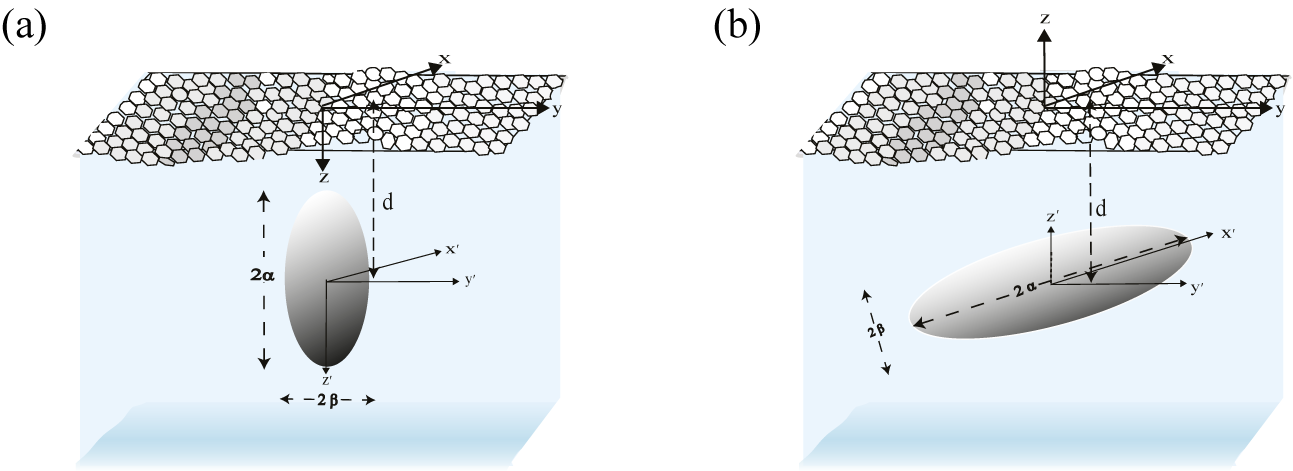
Here, it is considered that a prolate spheroidal body (Figure 1) is situated under the influence of a monochromatic incident wave field with linear amplitude A and frequency
$\omega $
 . For the axisymmetric configuration, the dependence on the wave-heading angle is excluded by using the perfect symmetry of the body. Without loss of generality, it is assumed that the wave propagates along the x-axis of the Cartesian coordinate system. So, the incident wave potential is written in polar coordinates as

where

Here,
$z= z{'}+d$
 , where
$z{'}$
 is fixed at the centre of the spheroidal body and
$\epsilon _{m}$
 = 1 for m = 0 and
$\epsilon _{m}$
 = 2 for
$m \geq 1$
 (details are given in Appendix B). Equations (6.1) and (6.2) can be expressed in prolate spheroidal coordinates by applying the following addition theorem suggested by Cooke [Reference Cooke8]:

where

is the Gegenbauer polynomial [Reference Cooke8]. If a is real and lies between the interval (-1,1), then
$a^{2}-1$
 gets replaced by
$1-a^{2}$
 . Using (6.3) and (6.4), we can transform (6.1) and (6.2) into the following:

where
$I_{n}$
 is the nth-order modified Bessel function of the first kind. Now, we use (6.5) to expand the incident wave potential, as

where

Prolate spheroid submerged at depth d below the ocean surface: (a) axisymmetric configuration; (b) nonaxisymmetric configuration.

Figure 1 Long description
The diagram consists of two panels, a and b, each depicting a three-dimensional volume of water with a textured surface representing the ocean.
Panel a shows the axisymmetric configuration. At the surface, a Cartesian coordinate system is established with x and y axes on the horizontal plane and a z axis pointing vertically downward. A prolate spheroid is positioned at a depth d below the surface. The spheroid is oriented vertically, with its long axis parallel to the z axis. A local coordinate system x prime, y prime, and z prime is centered within the spheroid. The vertical length of the spheroid is labeled 2 alpha, and its horizontal width is labeled 2 beta.
Panel b shows the nonaxisymmetric configuration. The surface coordinate system is identical, but the z axis points vertically upward. The prolate spheroid is submerged at the same depth d but is tilted at an angle. The local coordinate system x prime, y prime, and z prime is centered in the spheroid and rotated relative to the surface axes. In this tilted orientation, the long axis of the spheroid, labeled 2 alpha, follows the x prime axis, while the short axis, labeled 2 beta, is perpendicular to it.
6.1.2 Diffraction potential
For the particular boundary value problem, the diffraction potential is constructed analytically, using spheroidal harmonics, as

where
$D_{n}^{m}$
 are unknown coefficients that will be obtained by implementing the zero velocity condition on the wetted surface of the spheroidal body (detailed in Appendix B). With the help of (5.4), the two-dimensional Green’s function
$\tilde {G_{n}^{m}}(\eta ,\zeta )$
 can be written as

By using Taylor series expansion, we can expand the second integral in the right-hand-side (RHS) of (6.9) as

Equation (6.10) is simplified by using the purely analytic form of the integral in the RHS (see [Reference Gradshteyn and Ryzhik22]) as

where

Note that
$L_{n}^{m}(q)\neq 0 $
 only if
$n-m+q$
 is even. Using (6.10), the two-dimensional Green’s function
$\tilde {G_{n}^{m}}(\eta ,\zeta )$
 can be written as

The complex form of the Green’s function can be further simplified and finally can be written as

where

and

Equation (6.13) has been reduced to

with
$Y_{n}^{m}(p)=\sum _{q=m}^{\infty }X_{nq}^{mp}$
 .
The improper integral in (6.14) can be determined by using the residue theorem by choosing a proper contour. The corresponding expression for
$I_{p}^{m}(q)$
 can be evaluated by expressing the modified Bessel function of fractional order
$I_{p+1/2}(kc)$
 in terms of an associated ascending series, given by

6.2 The final linear system
Now, the ultimate form of velocity potentials mentioned in (6.6) and (6.8) have been introduced into the zero-velocity condition (see (2.7)) for
$u=u_{0}=\tanh ^{-1}(\beta /\alpha )$
 or equivalently
$\zeta =\zeta _0=\cosh (u_{0})$
 , and by using the orthogonality relations of both trigonometric and the associate Legendre functions of the first kind (see [Reference Abramowitz and Stegun1]), the final expression is reduced to

where
$\delta $
 denotes the Kronecker delta function, and
$F_{t}^{m}=\dot {P}_{t}^{m}(\zeta _0)/\dot {Q}_{t}^{m}(\zeta _0)$
 and the dot represents differentiation with respect to the argument. By solving the complex linear system in (6.15) numerically, we get the unknown coefficients
$D_{n}^{m}$
 . To perform the required computations, the linear system has to be truncated to account for a finite number of modes, N.
6.3 The nonaxisymmetric case
6.3.1 Incident wave potential
For the present case, the incident wave potential is taken in the following form:

where
$\theta {'}$
 represents the wave heading angle. For the nonaxisymmetric case, the orientation of the z-axis has been altered, pointing upwards such that
$z{'}=z+d$
 , where
$z{'}$
 denotes the vertical axis fixed at the centre of the spheroid. Now, the incident wave potential has been expanded into spheroidal harmonics by applying a relation originally provided by Havelock [Reference Havelock28],

where


where
$\epsilon _{m}$
 = 1 for
$m=0$
 and
$\epsilon _{m}$
 = 2 for
$m \geq 1$
 . As singularities arise at
$\theta {'}=\pm {\pi }/{2}$
 , we employ the following ascending series of Bessel functions to avoid the singularities:

The incident wave potential can be expressed as

where

and

6.3.2 Diffraction potential
To express the diffraction potential in terms of spheroidal harmonics, we simplify (5.5) as follows:

By using a similar argument as mentioned in (6.11), we can expand the second integral on the RHS of (6.20) in the following expression:

where
$I_{n}^{m}(q)=2(-1)^{m}H_{n}^{m}(q)$
 (see (6.12)).
Finally, we can write the Green’s function (5.4) in the following form:

where


where expressions of
$N_{l}(\theta )$
 and
$\tilde {N}_{l}(\theta )$
 are already defined in (6.16)–(6.17).
Again, we expand the Bessel function of the first kind in the ascending series to avoid the occurrence of singularities at
$\theta =\pm {\pi }/{2}$
 . Then, (6.22) and (6.23) are transformed into

and

The value of the improper integral in (6.24)–(6.25) can be determined using the residue theorem by choosing a proper contour.
6.4 The final linear system
Using the form of Green’s function given in (6.21), we can express the diffraction potential as

The Newmann boundary condition in (2.7) has been applied on the wetted surface of the body to obtain the unknown coefficients in (6.26). A set of linear systems has been acquired by employing the orthogonality relations of both the trigonometric and the associate Legendre functions of the first kind, on the real part of (2.7),


Here,
$\Re $
 and
$\Im $
 represent the real and imaginary parts of the variables, and
$F_{s}^{l}=\dot {P}_{s}^{l}(\zeta _0)/\dot {Q}_{s}^{l}(\zeta _0)$
 , where the dot represents differentiation with respect to the argument. Equations (6.27) and (6.28) were derived by using the cosine orthogonality relation. The same type of equations can be achieved by using the sine orthogonality relation, in which
$Y_{ns}^{ml}$
 and
$C_{s}^{l}$
 are replaced by
$\tilde {Y}_{ns}^{ml}$
 and
$\tilde {C_{s}^{l}}$
 , respectively. Real and imaginary parts of the unknown complex coefficient
$D_{n}^{m}$
 can be obtained by solving (6.27) and (6.28) together as a single set of linear equations. To perform the required calculations, the linear system has to be truncated to account for a finite number of modes, N. Once the velocity potentials are fully defined and the unknown coefficients are determined by solving the final linear systems, Section 6.5 uses these potentials to calculate the hydrodynamic forces and moments (surge, heave, sway and yaw) acting on the submerged body.
6.5 Hydrodynamic forces on the spheroid
The linear hydrodynamic pressure can be written as

By integrating (6.29) over the wetted surface of the body, the hydrodynamic forces exerted on the wetted surface of the spheroid can be attained as

and the moments with respect to the origin are provided as

where
$\vec {n}$
 is the unit normal vector,
$\vec {r}$
 suggests the radius vector from the origin to the surface of the spheroid and S indicates the wetted surface of the body. The components of the unit normal vector are described differently for axisymmetric and nonaxisymmetric cases. For the axisymmetric case, the components of n can be expressed as

whereas for the nonaxisymmetric case, the expression for
$n_{x}$
 and
$n_{z}$
 must be interchanged. The total differential area on the spheroid can be written as

By using all these important terms in (6.30), we can calculate the nondimensionalized form of both the surge and heave forces acting on the axisymmetric body in the form of

and

Here, the coefficients
$C_{n}^{m}$
 and
$D_{n}^{m}$
 are taken respectively from (6.7) and (6.8), and are obtained from the numerical solution of the linear system equation (6.15).
The following expressions of nondimensionalized exciting forces for the nonaxisymmetric case can be written as

The yaw exciting moment acting around the vertical axis of the horizontal prolate spheroidal body is given by the relation

where all the coefficients
$C_{n}^{m},\tilde {C_{n}^{m}},Y_{ns}^{ml}$
 and
$\tilde {Y_{ns}^{ml}}$
 are provided in (6.18), (6.19), (6.24) and (6.25), respectively.
To verify the analytical framework, Section 7 provides the numerical results. This section begins with a validation against existing literature to ensure accuracy of the present study, before engaging in a detailed discussion on how inertial surface parameter (E), coefficient of surface tension (M) and other parameters influence the hydrodynamic response.
7 Numerical results
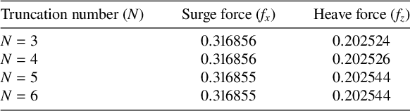
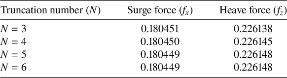
In this section, Mathematica has been used to solve the system of algebraic equations associated with both axisymmetric and nonaxisymmetric cases. As discussed earlier, the linear systems (6.15) and a combination of (6.27) and (6.28) have been truncated to a finite number of modes N to obtain the approximate solution for the potentials. The truncation number N = 6 has been considered, which is justified by Tables 1 and 2. In Table 1, we have computed the magnitude of surge force
$f_x$
 and heave force
$f_z$
 on the axisymmetric spheroid for different values of N, taking
$K\alpha =0.5$
 ,
$M/\alpha ^{2}=0.1$
 ,
$E/\alpha =0.05$
 ,
${\beta }/{\alpha }=0.4$
 . Similarly, the magnitude of surge force
$f_x$
 and heave force
$f_z$
 on the nonaxisymmetric spheroid have been represented in Table 2 for different values of N, considering the same values of the parameters as mentioned earlier with
$\theta {'}=30^{\circ }$
 . All the parameters have been nondimensionalized during the computation procedure.
Convergence of surge and heave forces (
$f_{x}$
 and
$f_{z}$
 ) on an axisymmetric prolate spheroid with
$\beta /\alpha =0.4$
 ,
$d/\alpha =1.25$
 ,
$M/\alpha ^{2}= 0.1$
 ,
$E/\alpha =0.05$
 for different values of N at
$K\alpha =0.5.$


Table 1 Long description
The table consists of three columns: Truncation number N, Surge force f sub x, and Heave force f sub z.
* Row 1: N equals 3, Surge force is 0.316856, Heave force is 0.202524.
* Row 2: N equals 4, Surge force is 0.316856, Heave force is 0.202526.
* Row 3: N equals 5, Surge force is 0.316855, Heave force is 0.202544.
* Row 4: N equals 6, Surge force is 0.316855, Heave force is 0.202544.
The data shows that the surge force stabilizes at 0.316855 and the heave force stabilizes at 0.202544 as N increases.
Convergence of surge and heave forces (
$f_{x}$
 and
$f_{z}$
 ) on a nonaxisymmetric prolate spheroid with
$\beta /\alpha =0.4$
 ,
$d/\alpha =1.25$
 ,
$E/\alpha =0.05\, M/\alpha ^{2}= 0.1$
 ,
$\theta {'}=30^{\circ }$
 for different values of N at
$K\alpha =0.5.$


Table 2 Long description
The table consists of three columns: Truncation number N, Surge force f sub x, and Heave force f sub z.
* At N = 3, the surge force is 0.180451 and the heave force is 0.226138.
* At N = 4, the surge force is 0.180450 and the heave force is 0.226145.
* At N = 5, the surge force is 0.180449 and the heave force is 0.226148.
* At N = 6, the surge force remains 0.180449 and the heave force remains 0.226148.
The data demonstrates numerical convergence for both forces as N reaches 5 and 6.
7.1 Validation
In the absence of brash ice and surface tension effects, specifically by setting
$M=0$
 and
$E=0$
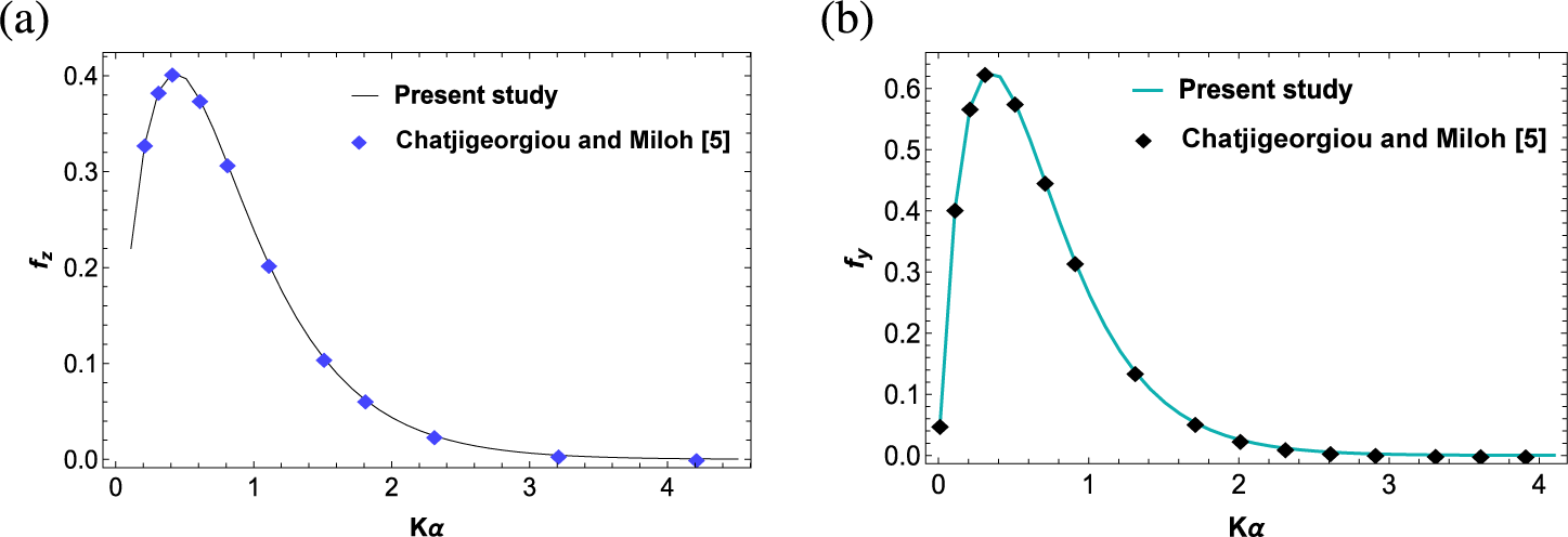
 in the brash-ice condition (2.5), the mathematical model simplifies to the classical diffraction problem of a submerged spheroid. Under these limiting conditions, the current formulation reduces to the problem previously investigated by Chatjigeorgiou and Miloh [Reference Chatjigeorgiou and Miloh5]. Consequently, the present results have been numerically validated in Figures 2(a) and 2(b) by comparing the results of Chatjigeorgiou and Miloh [Reference Chatjigeorgiou and Miloh5], and our result taking
$M/\alpha ^{2}=0$
 and
$E/\alpha =0$
 . In Figure 2(a), the magnitudes of heave force
$f_{z}$
 have been plotted against
$K\alpha $
 for an axisymmetric prolate spheroid submerged at a depth
$d/\alpha $
 = 2.5 with eccentricity
$\beta $
 /
$\alpha $
 = 0.7 and the magnitudes of sway force
$f_{y}$
 for a nonaxisymmetric prolate spheroid have been depicted graphically against
$K\alpha $
 for depth of submergence,
$ d/\alpha $
 = 3.0, with eccentricity
$\beta $
 /
$\alpha $
 = 0.9 and
$\theta {'}=30^{\circ }$
 in Figure 2(b). In the respective figures, the present results are represented by solid black and blue lines, while the data from the work of Chatjigeorgiou and Miloh [Reference Chatjigeorgiou and Miloh5] are shown by blue and black diamond symbols. From the subsequent figures, it can be noted that the present result perfectly matches with the result available from Chatjigeorgiou and Miloh [Reference Chatjigeorgiou and Miloh5], proving the accuracy of our present study.
(a) Comparison of the magnitude of heave force on axisymmetric prolate spheroid between the result of Chatjigeorgiou and Miloh [Reference Chatjigeorgiou and Miloh5], and our results with
$\beta $
 /
$\alpha $
 = 0.7,
$d/\alpha $
 = 2.5,
$M/\alpha ^{2}$
 = 0 and
$E/\alpha =0$
 . (b) Comparison of the magnitude of sway force on nonaxisymmetric prolate spheroid between the result of Chatjigeorgiou and Miloh [Reference Chatjigeorgiou and Miloh5], and our results with
$\beta $
 /
$\alpha $
 = 0.9,
$d/\alpha $
 = 3.0,
$\theta {'}=90^{\circ }$
 ,
$M/\alpha ^{2}$
 = 0 and
$E/\alpha =0$
 .

Figure 2 Long description
A two-panel figure labeled a and b.
Panel a shows a line graph of heave force f sub z on the vertical axis versus K alpha on the horizontal axis. The horizontal axis ranges from 0 to 4.5 and the vertical axis from 0.0 to 0.4. A solid black line representing the Present study shows a rapid increase from 0.2 to a peak of 0.4 at K alpha approximately 0.4, followed by an asymptotic decay toward zero. Blue diamond markers representing Chatjigeorgiou et al. 5 are plotted along the line, showing a high degree of correlation.
Panel b shows a line graph of sway force f sub y on the vertical axis versus K alpha on the horizontal axis. The horizontal axis ranges from 0 to 4 and the vertical axis from 0.0 to 0.6. A solid teal line representing the Present study rises sharply from near zero to a peak of approximately 0.62 at K alpha 0.4, then decays asymptotically. Black diamond markers representing Chatjigeorgiou et al. 5 are overlaid on the line, showing nearly identical values across the entire range.
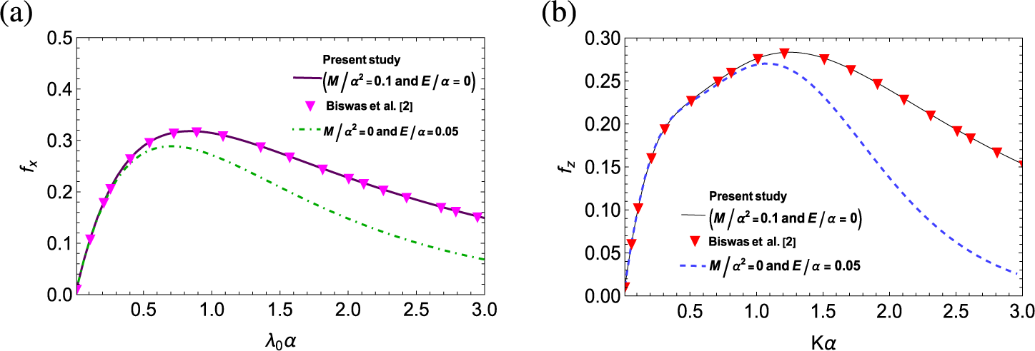
In Figure 3, the analytical framework is further validated by comparing the results of the present study with the existing literature of Biswas et al. [Reference Biswas, Das and De2], while also illustrating the distinct impacts of surface tension and brash ice on the hydrodynamic response. In Figure 3(a), the magnitudes of surge force
$f_{x}$
 have been plotted against
$\lambda _{0}\alpha $
 for an axisymmetric prolate spheroid (
$\beta $
 /
$\alpha $
 = 0.4) submerged at a depth
$d/\alpha $
 = 1.5 with
$M/\alpha ^{2}$
 = 0.1,
$E/\alpha =0$
 and the magnitudes of heave force
$f_{z}$
 for a nonaxisymmetric prolate spheroid (
$\beta $
 /
$\alpha $
 = 0.4) have been depicted graphically against
$K\alpha $
 for
$ d/\alpha $
 = 1.25,
$\theta {'}=30^{\circ }$
 with
$M/\alpha ^{2}$
 = 0.1,
$E/\alpha =0$
 in Figure 3(b). Purple and black lines indicate the present results, while magenta and red triangular markers represent the data points from the work of Biswas et al. [Reference Biswas, Das and De2] in Figures 3(a) and 3(b), respectively. The results show that in the absence of brash ice (
$E/\alpha =0$
 ), the magnitudes of the surge force on an axisymmetric spheroid and the heave force on a nonaxisymmetric spheroid perfectly match the data points provided by Biswas et al. [Reference Biswas, Das and De2]. These figures show two contrasting scenarios, a free surface with surface tension (
$M/\alpha ^2=0.1, E/\alpha =0$
 ) and a surface covered by brash ice without surface tension (
$M/\alpha ^2=0, E/\alpha =0.05$
 ). It is observed that the presence of brash ice (green and blue dashed lines in Figures 3(a) and 3(b), respectively) leads to a noticeable reduction in force magnitudes compared with the surface-tension-only case as the wavenumber increases.
(a) Comparison of the magnitude of surge force on axisymmetric prolate spheroid between the result of Biswas et al. [Reference Biswas, Das and De2] and our results with
$\beta $
 /
$\alpha $
 = 0.4, d/
$\alpha $
 = 1.5,
$M/\alpha ^{2}$
 = 0.1,
$E/\alpha =0$
 and the magnitude of surge force on an axisymmetric prolate spheroid (
$\beta $
 /
$\alpha $
 = 0.4) submerged at
$d/\alpha $
 = 1.5 with
$M/\alpha ^{2}$
 = 0,
$E/\alpha =0.05$
 . (b) Comparison of the magnitude of heave force on a nonaxisymmetric prolate spheroid between the result of Biswas et al. [Reference Biswas, Das and De2] and our results with
$\beta $
 /
$\alpha $
 = 0.4,
$d/\alpha $
 = 1.25,
$\theta {'}=30^{\circ }$
 ,
$M/\alpha ^{2}$
 = 0.1,
$E/\alpha =0$
 and the magnitude of heave force on a nonaxisymmetric prolate spheroid (
$\beta $
 /
$\alpha $
 = 0.4) submerged at
$d/\alpha $
 = 1.25 with
$M/\alpha ^{2}$
 = 0,
$E/\alpha =0.05$
 .

Figure 3 Long description
Two panels labeled a and b.
Panel a is a line graph showing surge force f sub x on the y-axis from 0.0 to 0.5 versus lambda sub 0 alpha on the x-axis from 0 to 3.0. A solid purple line representing the present study with M over alpha-squared equals 0.1 and E over alpha equals 0 rises to a peak of approximately 0.32 at lambda sub 0 alpha equals 0.8 before gradually declining. Pink downward-pointing triangles representing Biswas et al. align perfectly with this solid line. A second green dash-dot line representing M over alpha-squared equals 0 and E over alpha equals 0.05 follows a similar but lower trajectory, peaking at approximately 0.28 and declining more steeply.
Panel b is a line graph showing heave force f sub z on the y-axis from 0.00 to 0.30 versus K alpha on the x-axis from 0 to 3.0. A solid black line representing the present study with M over alpha-squared equals 0.1 and E over alpha equals 0 rises to a peak of 0.28 at K alpha equals 1.2. Red downward-pointing triangles representing Biswas et al. are plotted along this line. A blue dashed line representing M over alpha-squared equals 0 and E over alpha equals 0.05 follows the same initial rise but peaks earlier at K alpha equals 1.0 and drops significantly faster than the solid line as K alpha increases.
7.2 Results and discussion
In this subsection, the hydrodynamic response of a submerged spheroid in the presence of a brash ice cover is studied by analysing the forces and moment acting on the spheroid for different parameters, such as depth of submergence (d), eccentricity of the body (
$\beta $
 /
$\alpha $
 ), wave heading angle (
$\theta {'}$
 ). The discussion has been divided into two parts: vertical submergence (axisymmetric case) and horizontal submergence (nonaxisymmetric case) of the spheroid. At first, numerical results for the axisymmetric case have been illustrated, and in the latter part, the numerical results have been discussed for the nonaxisymmetric case. It should be noted that, with the presence of surface tension, there is no restriction on the value of
$K E$
 . Consequently, the figures have been plotted without any restriction on the range of
$K\alpha $
 .
Magnitudes of (a) surge and (b) heave force on a vertical prolate spheroidal body (
$\beta $
 /
$\alpha $
 = 0.4) submerged at
$d/\alpha $
 = 1.25 with coefficient of surface tension
$M/\alpha ^{2}$
 = 0.1 for different values of inertial surface parameter
$E/\alpha $
 .

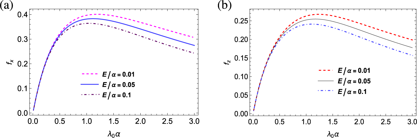
Figure 4 Long description
Two side-by-side line graphs labeled a and b.
Panel a shows surge force f sub x on the vertical axis from 0.0 to 0.4 and lambda sub 0 alpha on the horizontal axis from 0.0 to 3.0. Three curves rise sharply from the origin, peak near lambda sub 0 alpha equals 1.1, and then gradually decline. The top curve is a dashed magenta line for E over alpha equals 0.01. The middle curve is a solid blue line for E over alpha equals 0.05. The bottom curve is a dash-dot black line for E over alpha equals 0.1.
Panel b shows heave force f sub z on the vertical axis from 0.00 to 0.25 and lambda sub 0 alpha on the horizontal axis from 0.0 to 3.0. The curves follow a similar parabolic trend to panel a but with lower magnitudes. The top curve is a dashed red line for E over alpha equals 0.01. The middle curve is a solid black line for E over alpha equals 0.05. The bottom curve is a dash-dot blue line for E over alpha equals 0.1. In both panels, increasing the inertial surface parameter E over alpha results in a decrease in the force magnitude.
Magnitudes of (a) surge and (b) heave force on a vertical prolate spheroidal body (
$\beta $
 /
$\alpha $
 = 0.4) submerged at
$d/\alpha $
 = 1.25 with
$E/\alpha =0.05$
 for different values of coefficient of surface tension.

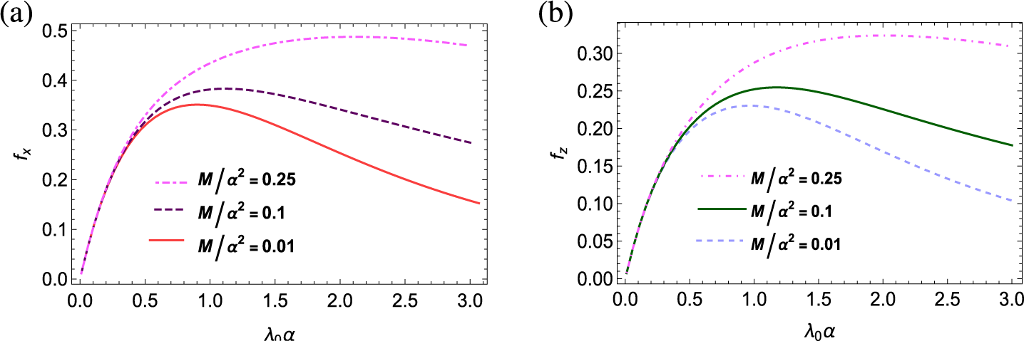
Figure 5 Long description
Two side-by-side line graphs labeled a and b.
Panel a, surge force f sub x. The x-axis is lambda sub 0 alpha ranging from 0.0 to 3.0. The y-axis is f sub x ranging from 0.0 to 0.5. Three curves represent different values of M all over alpha-squared.
- M all over alpha-squared equals 0.25 (pink dash-dot line) rises to a peak of approximately 0.49 at x equals 2.2 and slightly declines.
- M all over alpha-squared equals 0.1 (dark purple dashed line) peaks at approximately 0.38 at x equals 1.1 and declines to 0.28.
- M all over alpha-squared equals 0.01 (solid red line) peaks at approximately 0.35 at x equals 0.9 and declines more sharply to 0.15.
Panel b, heave force f sub z. The x-axis is lambda sub 0 alpha ranging from 0.0 to 3.0. The y-axis is f sub z ranging from 0.00 to 0.30.
- M all over alpha-squared equals 0.25 (pink dash-dot line) peaks at approximately 0.32 at x equals 2.0.
- M all over alpha-squared equals 0.1 (solid dark green line) peaks at approximately 0.25 at x equals 1.2.
- M all over alpha-squared equals 0.01 (light blue dashed line) peaks at approximately 0.23 at x equals 1.0.
In both graphs, higher surface tension coefficients result in higher peak force magnitudes occurring at higher wave numbers.
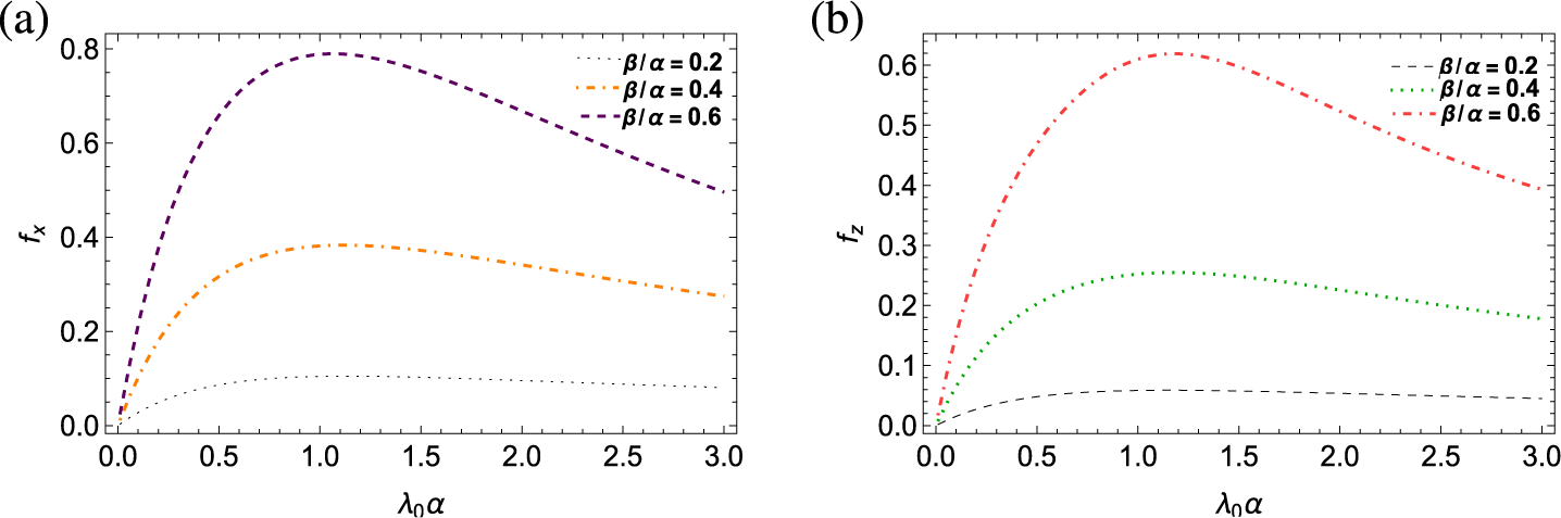
The magnitudes of both hydrodynamic forces (surge and heave) acting on the axisymmetric spheroid have been illustrated in Figures 4–7. For this part, the nondimensional values of the parameters have been considered as
$M/\alpha ^{2}$
 = 0.1,
$d/\alpha $
 = 1.25,
$E/\alpha =0.05$
 ,
$\beta $
 /
$\alpha $
 = 0.4 unless otherwise stated. In Figure 4, the exciting forces (surge and heave) have been plotted against the nondimensional wavenumber
$\lambda _{0}\alpha $
 for different values of the inertial surface parameter
$(E/\alpha = 0.01,0.05,0.1)$
 . The exciting forces, after attaining their peak for
$\lambda _{0}\alpha $
 lying in between 1 and 1.5, decrease for larger values of wavenumber. It is observed that the presence of brash ice has a significant impact on the forces acting on the spheroid. As the layer of brash ice gets heavier, that is, as the value of
$E/\alpha $
 increases, magnitudes of both the surge and heave forces decrease. However, for low wavenumber, the magnitudes of forces are almost identical. Notable differences in the forces occur only at frequencies near or exceeding the frequency corresponding to the maximum force. It is noticed that the presence of brash ice significantly reduces the magnitude of the forces acting on the spheroid. This reduction occurs because as
$E/\alpha $
 increases, the uniform layer of brash ice becomes heavier, which enhances the inertial resistance to wave motion.
Magnitudes of (a) surge and (b) heave force on a vertical prolate spheroidal body (
$\beta $
 /
$\alpha $
 = 0.4) with coefficient of surface tension M/
$\alpha ^{2}$
 = 0.1, inertial surface parameter
$E/\alpha =0.05$
 for different values of depth of submergence.

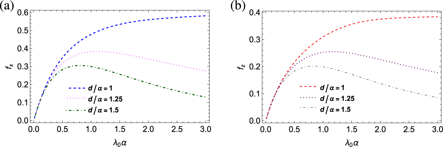
Figure 6 Long description
Two side-by-side line graphs labeled a and b. Both graphs share a horizontal x-axis labeled lambda sub 0 alpha ranging from 0.0 to 3.0.
Panel a displays surge force magnitude f sub x on the y-axis from 0.0 to 0.6. Three curves originate near the origin.
* The top curve, a blue dashed line for d forward slash alpha equals 1, increases asymptotically toward 0.6.
* The middle curve, a pink dotted line for d forward slash alpha equals 1.25, peaks at approximately 0.4 near x equals 1.0 and then gradually declines.
* The bottom curve, a green dash-dot line for d forward slash alpha equals 1.5, peaks at approximately 0.3 near x equals 0.7 and declines more sharply.
Panel b displays heave force magnitude f sub z on the y-axis from 0.0 to 0.4.
* The top curve, a red dashed line for d forward slash alpha equals 1, increases and levels off near 0.38.
* The middle curve, a black dotted line for d forward slash alpha equals 1.25, peaks near 0.25 and declines.
* The bottom curve, a black dash-dot line for d forward slash alpha equals 1.5, peaks near 0.2 and declines toward 0.1.
Magnitudes of (a) surge and (b) heave force on a vertical prolate spheroidal body with fixed submergence
$d/\alpha $
 = 1.25,
$M/\alpha ^{2}$
 = 0.1,
$E/\alpha =0.05$
 .

Figure 7 Long description
Two line graphs arranged horizontally. Both share an x axis labeled lambda sub 0 alpha ranging from 0.0 to 3.0.
Panel a on the left has a y axis labeled f sub x representing surge force magnitude ranging from 0.0 to 0.8. Three curves are shown.
- The lowest curve for beta over alpha equals 0.2 is a grey dotted line that rises slowly to a peak near 0.1 at x equals 1.2 and then slightly declines.
- The middle curve for beta over alpha equals 0.4 is an orange dash-dot line that rises to a peak near 0.4 at x equals 1.1 and gradually declines.
- The highest curve for beta over alpha equals 0.6 is a purple dashed line that rises sharply to a peak near 0.8 at x equals 1.1 and then declines toward 0.5.
Panel b on the right has a y axis labeled f sub z representing heave force magnitude ranging from 0.0 to 0.6.
- The lowest curve for beta over alpha equals 0.2 is a grey dashed line peaking near 0.05.
- The middle curve for beta over alpha equals 0.4 is a green dotted line peaking near 0.25 at x equals 1.2.
- The highest curve for beta over alpha equals 0.6 is a red dash-dot line peaking near 0.62 at x equals 1.2 and then declining toward 0.4.
This increased inertia dampens the wave amplitudes and reduces the energy transmitted to the submerged prolate spheroid, leading to lower hydrodynamic forces. With the increment of E, the positive root of the dispersion relation
$L(k)\equiv k(1-KE+Mk^2)-K=0$
 shifts, altering the wavenumber
$\lambda _{0}$
 , which in turn affects the incident and diffracted wave potentials. The resulting decrease in wave energy transmitted to the spheroid reduces the pressure gradients that drive
$f_{z}$
 and
$f_{x}$
 . Figure 5 depicts both exciting forces (surge and heave) against the wavenumber
$\lambda _{0}\alpha $
 for different values of the coefficient of surface tension
$(M/\alpha ^{2}=0.01, 0.1, 0.25)$
 . The presence of surface tension not only guarantees the wave propagation for every frequency, but also has a great impact on the magnitude of forces acting on the body. Figure 5 demonstrates that the magnitudes of both hydrodynamic forces increase as the coefficient of surface tension
$M/\alpha ^{2}$
 increases. Similar observations were also reported by Biswas et al. [Reference Biswas, Das and De2]. Also, after attaining the peak value, a substantial decrease in the magnitude of forces is not observed for higher values of surface tension. Figures 6(a) and 6(b) represent the magnitudes of surge and heave forces, respectively, against wavenumber
$\lambda _{0}\alpha $
 for different values of depth of submergence (
$d/\alpha = 1, 1.25, 1.5$
 ). From Figure 6, it can be concluded that when the spheroidal body is closer to the ocean surface covered by brash ice (that is,
$d/\alpha $
 = 1), the magnitudes of both the forces (surge and heave) reach higher values. The findings reveal that, compared with the heave force, the magnitudes of surge force attain greater values. It is also noticed that when the spheroidal body is closer to the ocean surface, the decrease in the magnitudes of both surge and heave forces is very minimal for greater wavenumbers. Moreover, for
$d/\alpha $
 = 0.1, both the forces are nondecreasing for increasing wavenumbers. Hydrodynamic forces (surge and heave) against
$\lambda _{0}\alpha $
 have been depicted in Figures 7(a) and 7(b) for various eccentricities of the body
$\beta $
 /
$\alpha $
 (
$=0.2,0.4,0.6$
 ). It is observed that the spheroid experiences a greater heave and surge force with the increase in its eccentricity, being consistent with the findings of Chatjigeorgiou and Miloh [Reference Chatjigeorgiou and Miloh5].
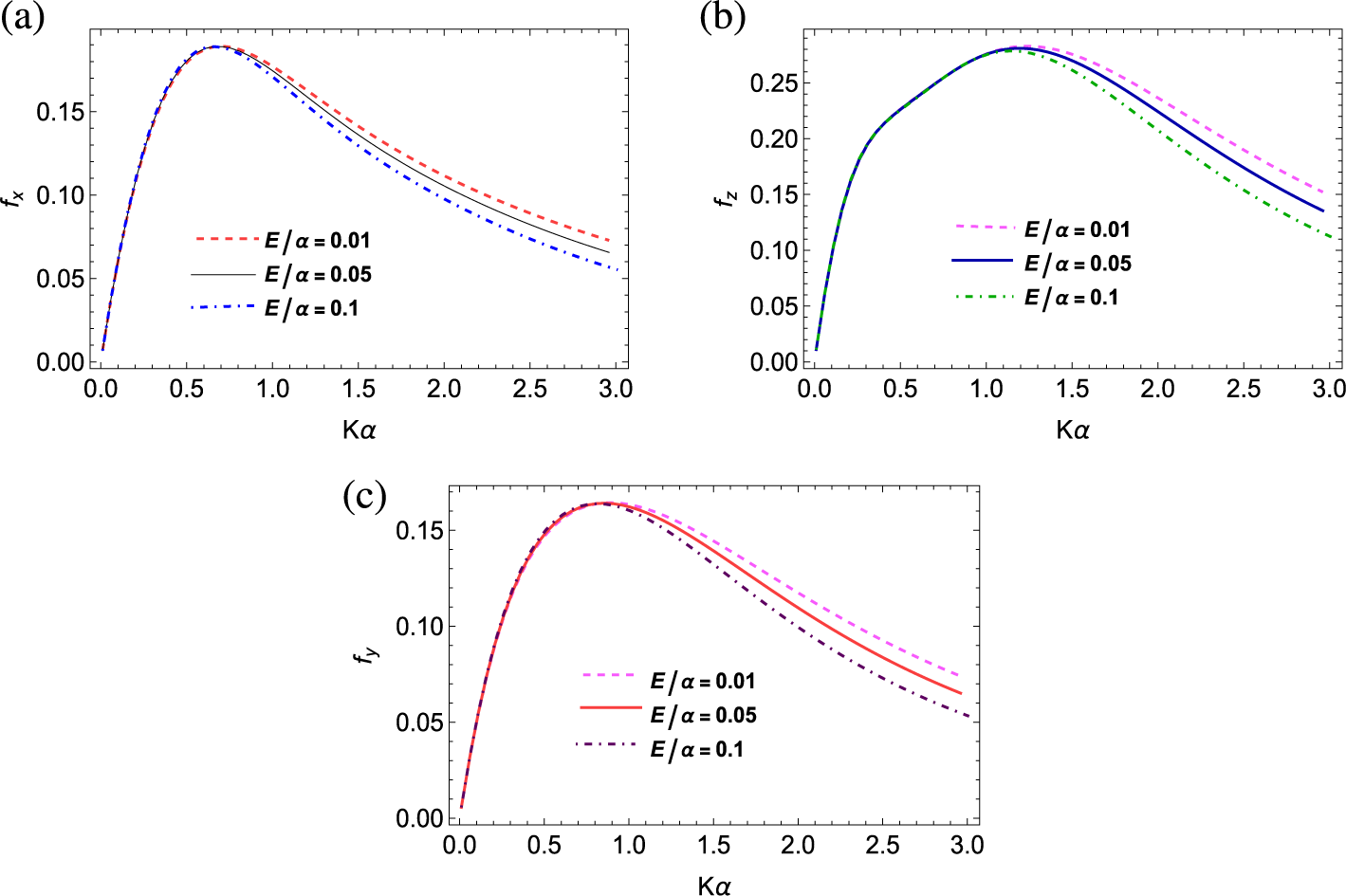
Now, we will discuss the hydrodynamic properties of a nonaxisymmetric prolate spheroid. For horizontal submergence of the spheroid, the sway force has been also obtained along with the heave and surge forces. An illustration of variations in the magnitudes of the surge, heave and sway forces is shown in Figures 8–12, considering the nondimensional values of the parameters as
$M/\alpha ^{2}$
 = 0.1,
$d/\alpha $
 = 1.25,
$E/\alpha =0.05$
 ,
$\beta $
 /
$\alpha $
 = 0.4 and
$\theta {'}=30^{\circ }$
 unless otherwise stated. In Figures 8(a), 8(b) and 8(c), the magnitudes of the surge, heave and sway forces have been plotted against
$K\alpha $
 for different values of inertial surface parameter
$E/\alpha (= 0.01,0.05,0.1)$
 , respectively. Similar to the vertical submergence, here also, it has been observed that a heavier layer of brash ice decreases the magnitudes of surge, heave and sway forces for moderate to high frequencies. However, for low wave frequencies, the magnitude of forces is almost indifferent. Significant changes can be observed for higher wave frequencies after the peak value of the exciting forces is reached. It is noteworthy that the magnitude of surge force is almost the same for different ice densities for low frequencies, up to the attainment of the peak value. Similar phenomena have also been observed for the sway force. Evidently, the magnitudes of the heave force reach greater values in comparison with the surge and sway forces.
Magnitudes of (a) surge, (b) heave and (c) sway force on a horizontal prolate spheroidal body (
$\beta $
 /
$\alpha $
 = 0.4) with different values of inertial surface parameter
$E/\alpha $
 , coefficient of surface tension
$M/\alpha ^{2}$
 = 0.1, wave heading angle
$\theta {'}=30^{\circ }$
 , fixed submergence
$d/\alpha $
 = 1.25.

Figure 8 Long description
A three-panel set of line graphs labeled a, b, and c. All graphs share a common x-axis labeled K alpha ranging from 0.0 to 3.0. Each graph contains three curves representing E over alpha values of 0.01, 0.05, and 0.1.
* Panel a: The y-axis is f sub x (surge force) ranging from 0.00 to 0.15. All three curves rise sharply from the origin to a peak near K alpha equals 0.7. After the peak, the curves diverge as they descend. The curve for E over alpha equals 0.01 (dashed red) remains highest, followed by 0.05 (solid black), and 0.1 (dash-dot blue) is the lowest.
* Panel b: The y-axis is f sub z (heave force) ranging from 0.00 to 0.25. The curves peak at approximately K alpha equals 1.2. The dashed pink line (0.01) is the highest after the peak, the solid blue line (0.05) is in the middle, and the dash-dot green line (0.1) is the lowest.
* Panel c: The y-axis is f sub y (sway force) ranging from 0.00 to 0.15. The curves peak near K alpha equals 0.8. Similar to the other panels, the dashed pink line (0.01) shows the highest magnitude during the descent, followed by the solid red line (0.05) and the dash-dot purple line (0.1).
Magnitudes of (a) surge, (b) heave and (c) sway force on a horizontal prolate spheroidal body (
$\beta $
 /
$\alpha $
 = 0.4) with inertial surface parameter
$E/\alpha =0.05$
 , for different values of coefficient of surface tension M, wave heading angle
$\theta {'}=30^{\circ }$
 , fixed submergence
$d/\alpha $
 = 1.25.

Figure 9 Long description
A three-panel set of line graphs labeled a, b, and c. All panels share a common x-axis labeled K alpha, ranging from 0.0 to 3.0. Each panel contains three curves representing different values of M all over alpha-squared: 0.01 (dotted line), 0.1 (dashed line), and 0.25 (dash-dot line).
* Panel a: The y-axis is f sub x (surge force). All three curves rise sharply from the origin to a peak of approximately 0.19 at K alpha equals 0.7. After the peak, the curves diverge: the 0.01 curve decays most rapidly toward 0.02, while the 0.25 curve decays most slowly, ending near 0.10.
* Panel b: The y-axis is f sub z (heave force). The curves rise from the origin and peak at different points. The 0.01 curve peaks earliest at 0.27 around K alpha equals 1.0. The 0.25 curve peaks latest at 0.29 around K alpha equals 1.4. Higher values of M all over alpha-squared result in higher force magnitudes at higher wave numbers.
* Panel c: The y-axis is f sub y (sway force). Similar to panel a, the curves overlap during the initial rise to a peak of 0.16 at K alpha equals 0.8. Post-peak, the curves diverge significantly: the 0.01 curve drops to near 0.02, whereas the 0.25 curve remains higher, ending near 0.10 at the x-axis limit.
Magnitudes of (a) surge, (b) heave and (c) sway force on a horizontal prolate spheroidal body (
$\beta $
 /
$\alpha $
 = 0.4) with wave heading angle
$\theta {'}=30^{\circ }$
 ,
$M/\alpha ^{2}$
 = 0.1, inertial surface parameter
$E/\alpha =0.05$
 for different values of depth of submergence.

Figure 10 Long description
A three-panel line graph arrangement labeled a, b, and c. All panels share a common x-axis labeled lambda sub 0 alpha, ranging from 0.0 to 3.0.
Panel a, top-left, shows surge force f sub x on the y-axis from 0.00 to 0.20. Three curves rise to a peak around lambda sub 0 alpha equals 0.7 and then decay. The highest peak is for d forward slash alpha equals 1 (pink dashed line), followed by d forward slash alpha equals 1.25 (red dotted line), and the lowest is d forward slash alpha equals 1.5 (blue dash-dot line).
Panel b, top-right, shows heave force f sub z on the y-axis from 0.00 to 0.35. The curves show a broader peak. The blue dashed line (d forward slash alpha equals 1) reaches the highest peak near 0.35 at lambda sub 0 alpha equals 1.5. The black dotted line (d forward slash alpha equals 1.25) peaks near 0.28. The green dash-dot line (d forward slash alpha equals 1.5) peaks earliest and lowest near 0.24.
Panel c, bottom-center, shows sway force f sub y on the y-axis from 0.00 to 0.20. The green dashed line (d forward slash alpha equals 1) has the highest peak near 0.20 at lambda sub 0 alpha equals 1.2. The purple dash-dot line (d forward slash alpha equals 1.25) peaks near 0.16. The pink dotted line (d forward slash alpha equals 1.5) has the lowest peak near 0.14.
Magnitudes of (a) surge, (b) heave and (c) sway force on a horizontal prolate spheroidal body with fixed submergence
$d/\alpha $
 = 1.25,
$M/\alpha ^{2}$
 = 0.1,
$\theta {'}=30^{\circ }$
 and
$E/\alpha =0.05$
 for varying eccentricity of the spheroid.

Figure 11 Long description
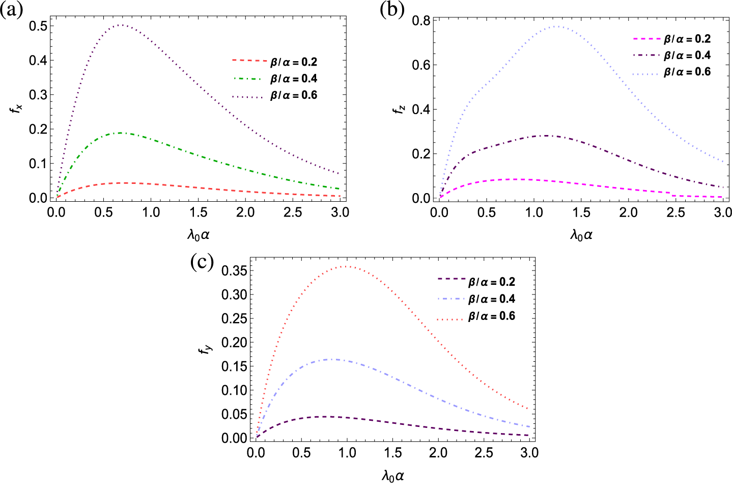
A three-panel set of line graphs labeled a, b, and c. All graphs share a common x-axis labeled lambda sub 0 alpha ranging from 0.0 to 3.0. Each graph contains three curves representing beta forward slash alpha values of 0.2, 0.4, and 0.6.
* Panel a: The y-axis is f sub x, representing surge force, ranging from 0.0 to 0.5. All curves show a rapid initial increase to a peak followed by a gradual decay. The peak for beta forward slash alpha equals 0.6 is the highest at approximately 0.5 when x is 0.7. The peak for 0.4 is lower at 0.2, and 0.2 is the lowest at approximately 0.05.
* Panel b: The y-axis is f sub z, representing heave force, ranging from 0.0 to 0.8. The curves follow a similar bell-shaped trend but with peaks shifted further right compared to panel a. The peak for beta forward slash alpha equals 0.6 reaches nearly 0.8 at x equals 1.2. The peak for 0.4 is at 0.3, and 0.2 is at 0.1.
* Panel c: The y-axis is f sub y, representing sway force, ranging from 0.0 to 0.35. The curves peak between x equals 0.8 and 1.0. The highest curve for beta forward slash alpha equals 0.6 peaks at 0.35. The curve for 0.4 peaks at 0.17, and the curve for 0.2 peaks at 0.05.
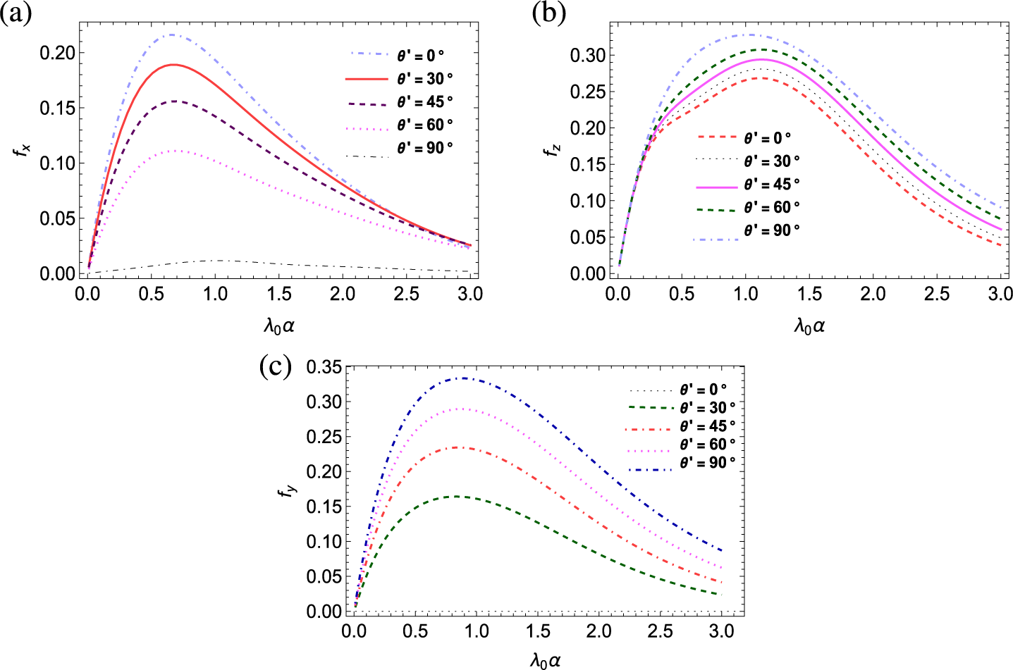
Magnitudes of (a) surge, (b) heave and (c) sway force on a horizontal prolate spheroidal body (
$\beta $
 /
$\alpha $
 = 0.4) for various wave heading angles
$\theta {'}$
 with fixed submergence
$d/\alpha $
 = 1.25,
$ M/\alpha ^{2}$
 = 0.1 and
$E/\alpha =0.05$
 .

Figure 12 Long description
The figure consists of three panels labeled a, b, and c. All panels share a common x-axis labeled lambda sub 0 alpha ranging from 0.0 to 3.0.
Panel a, located at the top left, shows f sub x on the y-axis from 0.00 to 0.20. It contains five curves for theta prime values. The curve for 0 degrees is the highest, peaking near 0.22 at lambda sub 0 alpha equals 0.7. As theta prime increases to 30, 45, and 60 degrees, the peak magnitude decreases sequentially. The curve for 90 degrees is nearly flat and remains near zero.
Panel b, located at the top right, shows f sub z on the y-axis from 0.00 to 0.30. The curves follow a similar parabolic trend, peaking between lambda sub 0 alpha values of 1.0 and 1.5. Here, the 90 degree curve is the highest, followed by 60, 45, 30, and 0 degrees in descending order of magnitude.
Panel c, located at the bottom center, shows f sub y on the y-axis from 0.00 to 0.35. The 90 degree curve is the highest, peaking at approximately 0.33. The magnitudes decrease as theta prime decreases to 60, 45, and 30 degrees. The 0 degree curve is a flat baseline at zero.
In all panels, the curves converge toward lower values as lambda sub 0 alpha approaches 3.0.
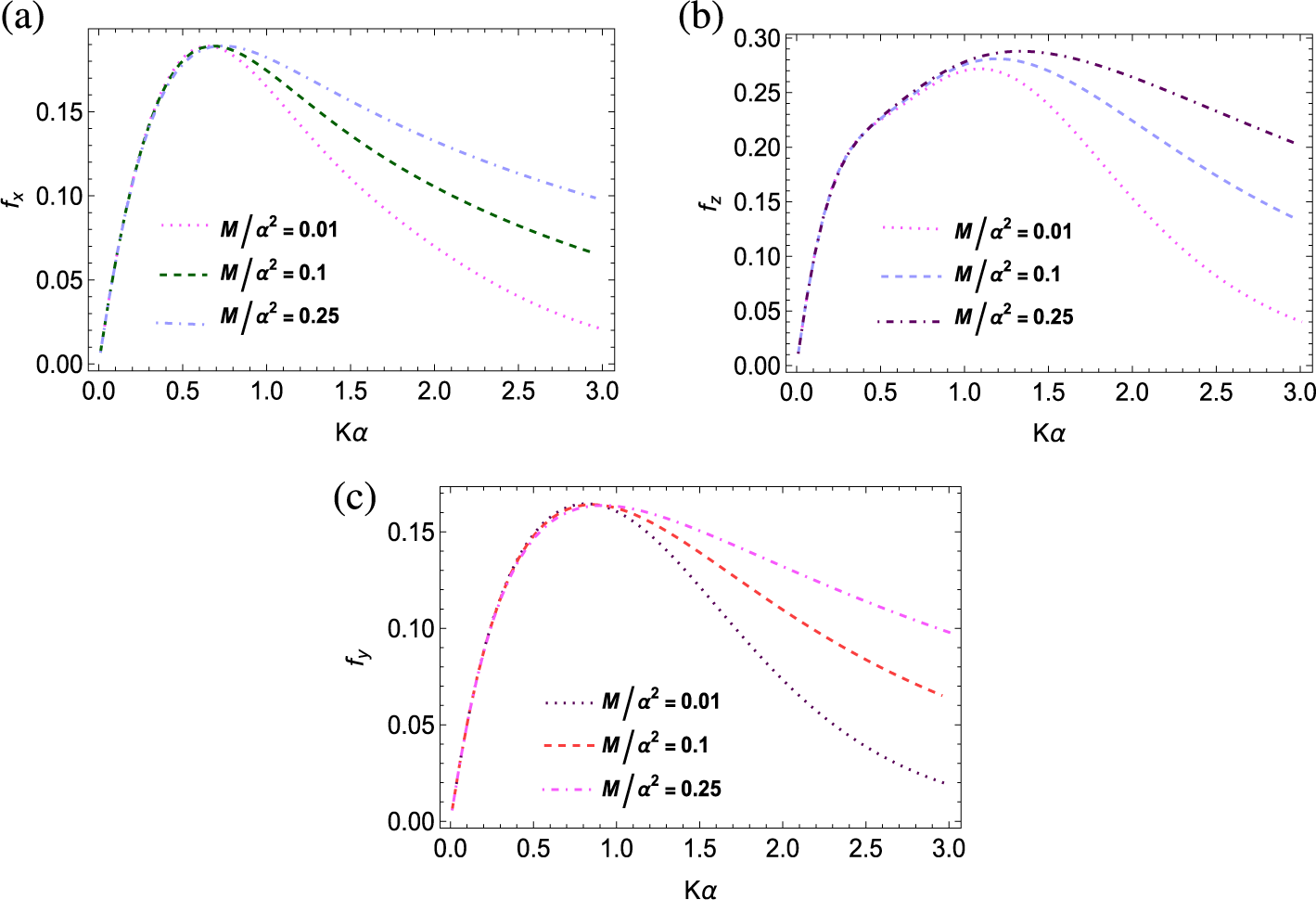
In Figures 9(a), 9(b) and 9(c), the effect of surface tension on the magnitude of all three forces has been demonstrated. The graphs have been plotted against
$K\alpha $
 for different values of the surface tension coefficient
$(M/\alpha ^{2}=0.01,0.1,0.25)$
 . From these figures, it can be concluded that as the surface tension of water (
$M/\alpha ^{2}$
 ) increases, the magnitudes of surge, heave and sway forces also increase, although the difference is significant only for moderate and high frequencies. Also, it is crucial to note that for very low surface tension, all three forces decline sharply after attaining peak value.
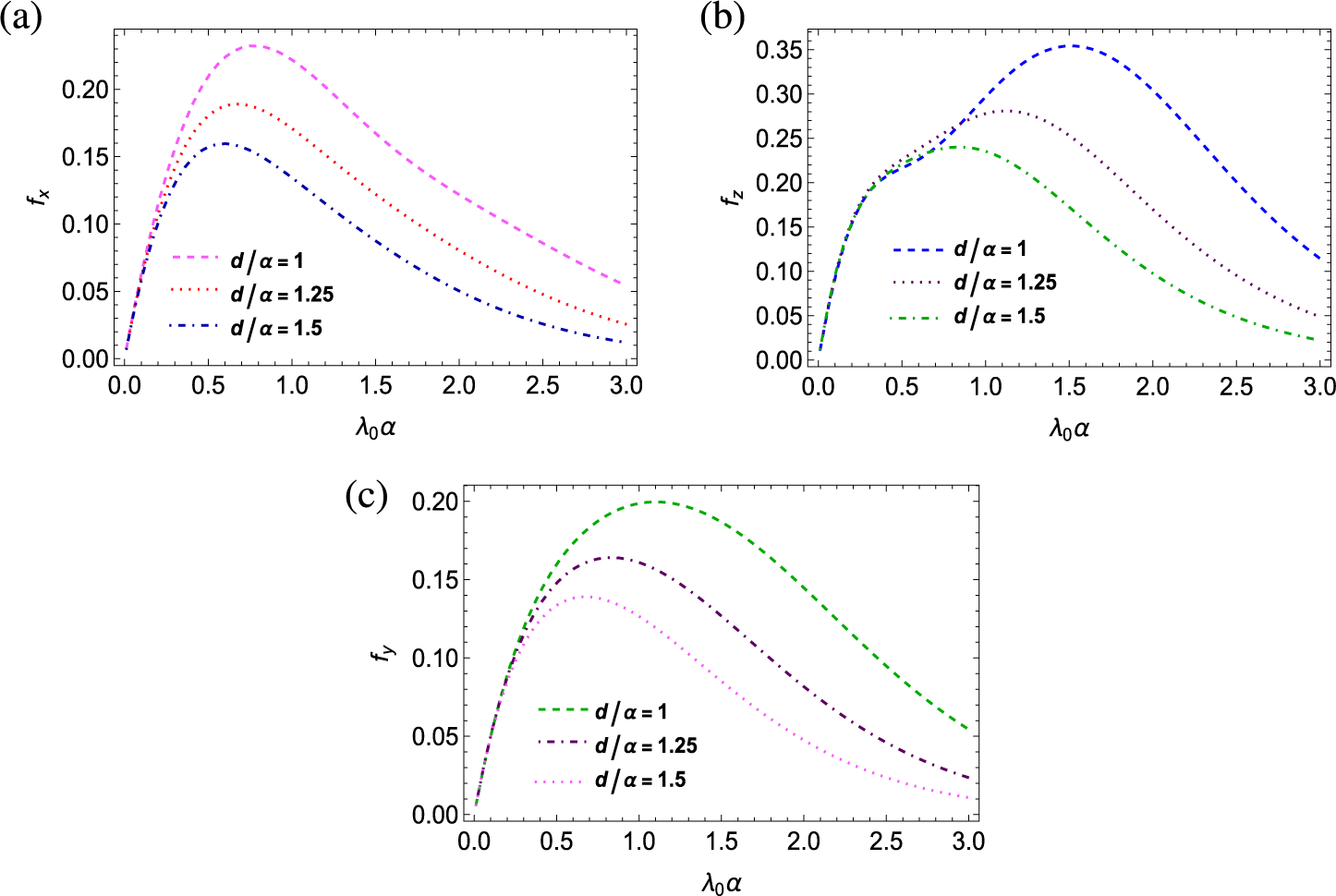
In Figures 10(a), 10(b) and 10(c), magnitudes of surge, heave and sway forces have been depicted against
$\lambda _{0}\alpha $
 for different values of depth of submergence
$d/\alpha =1,1.25,1.5$
 . When the spheroidal body is closer to the ocean surface covered by brash ice (that is,
$d/\alpha $
 = 1), magnitudes of all three forces (surge, heave and sway forces) attain greater values than in the case where the spheroid is submerged relatively deeper (that is,
$d/\alpha $
 = 1.25 and
$d/\alpha $
 = 1.5), as illustrated in Figure 10. Moreover, the peak of the heave force is attained at a much larger frequency. Numerical computations reveal that at some wavenumbers (between 0.5 and 1), the heave force is less when it is situated closer to the ice layer.
Figure 11 depicts the impact of the geometry of the structure on the hydrodynamic loads. It is evident from Figures 11(a), 11(b) and 11(c) that all three types of hydrodynamic loading components increase for larger eccentricity (that is,
$\beta $
 /
$\alpha $
 = 0.2, 0.4, 0.6) of the spheroid. However, the increase in the magnitude of the heave force is significantly higher than the increase in the surge and sway force components when the eccentricity of the spheroid increases. Figure 12 shows that the surge force decreases when the incident angle (
$\theta {'} =0^{\circ },30^{\circ },45^{\circ },60^{\circ },90^{\circ })$
 increases up to the normal incidence, while the heave and sway forces increase as the incident wave angle increases. It is interesting to note that the sway force exceeds the heave force acting on the body for normal incidence.
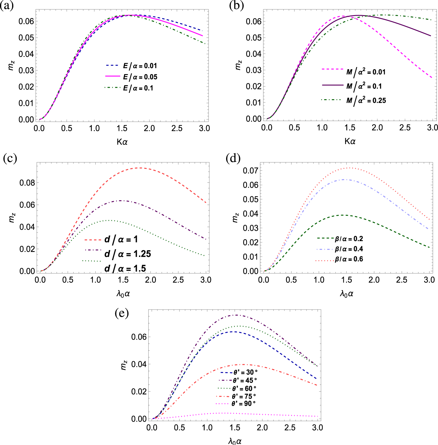
Numerical simulation for yaw moment has been depicted in Figure 13 for various values of the brash ice parameter, surface tension coefficient, depth of submergence, wave heading angle and eccentricity. Here, the values of different parameters have been considered as
$E/\alpha =0.05$
 ,
$M/\alpha ^{2}= 0.1$
 ,
$\beta $
 /
$\alpha $
 = 0.4,
$\theta {'}=30^{\circ }$
 and
$ d/\alpha $
 = 1.25, unless otherwise mentioned. The impact of the layer of brash ice at the topmost surface of the ocean, having a surface tension effect, on the yaw moment around the vertical axis is shown in Figures 13(a) and 13(b). Here, the magnitudes of the yaw moment have been depicted against
$K\alpha $
 for different values of inertial surface parameter (
$E/\alpha =0.01,0.05,0.1$
 ). The existence of brash ice does not significantly alter the peak value of the yaw moment, though the frequency at which the peak occurs shifts to a lower value as the brash ice density increases. Similar phenomena have been observed for the changes in the surface tension parameter, but instead of shifting to a lower wavenumber, the peak shifts to a higher wavenumber when the surface tension increases. In addition, it has been observed that the magnitude of the yaw moment is significantly reduced at high wavenumbers due to a heavy layer of brash ice. However, in the presence of a light layer of brash ice, the reduction of yaw moment is much less for high wavenumbers in comparison to the case of the free surface. In Figure 13(c), the magnitudes of yaw moment have been depicted against
$\lambda _{0}\alpha $
 for different values of depth of submergence
$d/\alpha =1,1.25,1.5$
 and in Figure 13(d), it has been observed for different values of
$\beta $
 /
$\alpha $
 = 0.2, 0.4, 0.6. These two figures indicate that the moment acting on the spheroidal body decreases as the body’s eccentricity decreases and as the depth of submergence increases. A compelling aspect is that after achieving its maximum value, the magnitude of the yaw moment rapidly decreases with the increasing value of eccentricity of the body. The wave heading angles
$30^{\circ }$
 ,
$45^{\circ }$
 ,
$60^{\circ }$
 ,
$75^{\circ }$
 and
$90^{\circ }$
 have been considered, and the magnitude of yaw moment has been represented graphically against
$\lambda _{0}\alpha $
 in Figure 13(e). It is evident that for increasing
$\lambda _{0}\alpha $
 , the magnitudes of yaw moment for a heading angle of
$45^{\circ }$
 is higher than other observed heading angle values of
$75^{\circ }$
 and
$90^{\circ }$
 as well as
$30^{\circ }$
 and
$60^{\circ }$
 , as illustrated in Figure 13(e). The value of the yaw moment around the vertical axis of the spheroid almost vanishes for
$90^{\circ }$
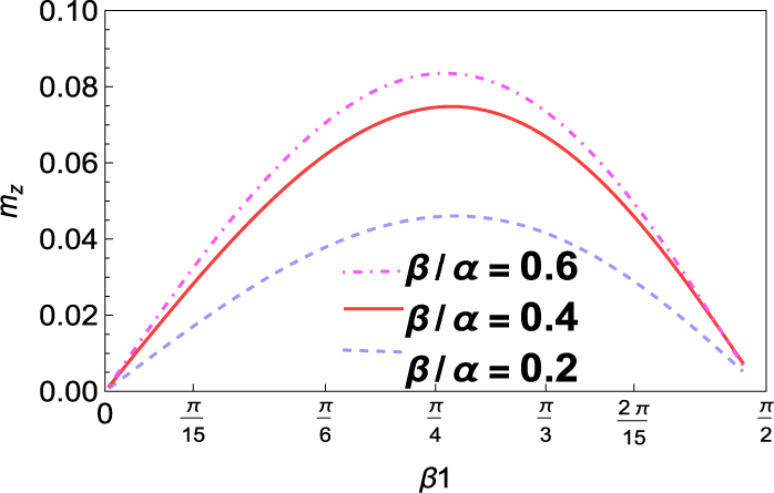
 . To further analyse the effect of wave heading angle, in Figure 14,
$m_z$
 has been depicted against
$\theta {'}$
 for different values of eccentricities (
$\beta /\alpha $
 = 0.2, 0.4, 0.6). Clearly, the yaw moment is highest near
$\theta {'}=\pi /4$
 , and it almost vanishes near
$\theta {'}=0$
 and
$\theta {'}= \pi /2$
 . The precise wave heading angle for which the maximum occurs is
$\theta {'}=\pi /3.8$
 .
Magnitudes of yaw moment on a horizontal prolate spheroidal body with (a)
$\beta $
 /
$\alpha $
 = 0.4, different values of inertial surface parameter
$E/\alpha $
 , wave heading angle
$\theta {'}=30^{\circ }$
 , fixed submergence
$d/\alpha $
 = 1.25, M/
$\alpha ^{2}$
 = 0.1; (b)
$\beta $
 /
$\alpha $
 = 0.4, different values of coefficient of surface tension
$M/\alpha ^{2}$
 , wave heading angle
$\theta {'}=30^{\circ }$
 , fixed submergence
$d/\alpha $
 = 1.25,
$E/\alpha =0.05$
 ; (c)
$\beta $
 /
$\alpha $
 = 0.4, wave heading angle
$\theta {'}=30^{\circ }$
 ,
$M/\alpha ^{2}$
 = 0.1,
$E/\alpha =0.05$
 ; (d) various eccentricity and wave heading angle
$\theta {'}=30^{\circ }$
 , fixed submergence
$d/\alpha $
 = 1.25,
$M/\alpha ^{2}$
 = 0.1,
$E/\alpha =0.05$
 ; (e)
$\beta $
 /
$\alpha $
 = 0.4, fixed submergence
$d/\alpha $
 = 1.25,
$M/\alpha ^{2}$
 = 0.1,
$E/\alpha =0.05$
 , different values of wave heading angles.

Figure 13 Long description
The figure consists of five panels labeled a through e. All panels feature the yaw moment m sub z on the vertical Y-axis, ranging from 0.00 to approximately 0.08.
Panel a: Plots m sub z against K alpha. Three curves represent inertial surface parameter E forward slash alpha values of 0.01 (dashed blue), 0.05 (solid magenta), and 0.1 (dash-dot green). All curves peak near K alpha equals 1.5, with higher E forward slash alpha values resulting in a lower peak and faster decay.
Panel b: Plots m sub z against K alpha. Three curves represent surface tension coefficient M forward slash alpha squared values of 0.01 (dashed magenta), 0.1 (solid purple), and 0.25 (dash-dot green). As M forward slash alpha squared increases, the peak of the curve shifts to the right and the magnitude remains higher at larger K alpha values.
Panel c: Plots m sub z against lambda sub 0 alpha. Three curves represent submergence d forward slash alpha values of 1 (dashed red), 1.25 (dash-dot purple), and 1.5 (dotted green). Increasing submergence significantly reduces the magnitude of the yaw moment across all wave frequencies.
Panel d: Plots m sub z against lambda sub 0 alpha. Three curves represent eccentricity beta forward slash alpha values of 0.2 (dashed green), 0.4 (dash-dot blue), and 0.6 (dotted red). Higher eccentricity leads to a higher peak yaw moment.
Panel e: Plots m sub z against lambda sub 0 alpha for different wave heading angles theta prime. Curves represent 30 degrees (dashed blue), 45 degrees (dash-dot green), 60 degrees (dotted black), 75 degrees (dash-dot-dot red), and 90 degrees (dotted magenta). The yaw moment is highest at 60 degrees and lowest at 90 degrees.
Magnitudes of yaw moment on horizontal prolate spheroidal body for varying eccentricity of the spheroid with fixed submergence
$d/\alpha $
 = 1.25,
$K\alpha =1.5$
 ,
$M/\alpha ^{2}$
 = 0.1 and
$E/\alpha =0.05$
 .

Figure 14 Long description
The horizontal X axis is labeled beta 1 and ranges from 0 to pi all over 2, with intermediate tick marks at pi all over 15, pi all over 6, pi all over 4, pi all over 3, and 2 pi all over 15. The vertical Y axis is labeled m sub z and ranges from 0.00 to 0.10 in increments of 0.02. Three curves originate at the origin (0,0) and follow a parabolic arc, peaking near beta 1 equals pi all over 4 before descending toward pi all over 2.
* The uppermost curve is a pink dash-dot line representing beta forward slash alpha equals 0.6, reaching a peak m sub z of approximately 0.08.
* The middle curve is a solid red line representing beta forward slash alpha equals 0.4, reaching a peak m sub z of approximately 0.075.
* The lowermost curve is a light blue dashed line representing beta forward slash alpha equals 0.2, reaching a peak m sub z of approximately 0.045.
A legend is located in the lower right quadrant of the plot area corresponding to these three values.
8 Conclusion
In the present work, the semi-analytical and numerical solutions for the wave diffraction problem by a prolate spheroid (both vertical and horizontal) submerged beneath a layer of brash ice in an infinitely deep water region have been formulated, using the linear theory incorporating the effect of surface tension at the free surface. The brash ice has been considered as a layer of uniform noninteracting ice particles, modelled as an inertial surface. The spheroidal coordinate system has been introduced to use the symmetry of the body and spheroidal harmonics have been used to express the potentials. The diffraction potential has been decomposed in terms of the multipoles of Green’s function, obtained by employing Havelock’s theorem for the ultimate image singularity system for spheroidal harmonics. Multipoles of Green’s function are derived for both axisymmetric and nonaxisymmetric cases. The residue theorem has been employed to reduce the subsequent mathematical expressions by choosing proper contours. The surge, heave and sway forces, along with the yaw moment exerted on the prolate spheroid, have been illustrated numerically, and the effect of various parameters on these quantities has been analysed. The following key observations were made during the numerical simulation regarding the hydrodynamic forces and moments acting on the body.
-
• Numerical results demonstrate that the existence of brash ice at the free surface significantly reduces the magnitudes of the forces acting on the spheroid.
-
• The rate at which the magnitude of forces decreases at higher wavenumbers is lower compared with the free surface case.
-
• Brash ice affects different orientations uniquely; while the rate of force reduction at high wavenumbers is very low and nearly constant for different densities of brash ice for axisymmetric spheroids, forces on nonaxisymmetric (horizontal) spheroids are more significantly reduced at higher frequencies as ice density increases.
-
• In contrast, the presence of surface tension not only guarantees the existence of a propagating wave, but due to an increase in the surface tension, it also experiences more force being acted on its surface with an increased yaw moment at moderate to high frequencies.
-
• The peak value of the moment does not significantly change due to different densities of brash ice.
-
• At some frequencies, mainly in the low to moderate range, a relatively lower yaw moment has been observed for an increase in the coefficient of surface tension.
-
• When the spheroid (both axisymmetric and nonaxisymmetric) is present near the free surface, the magnitudes of forces and moments are considerably higher, and the same can be observed for an increase in the eccentricity of the spheroid.
-
• The incoming wave produces the highest heave force at normal incidence.
-
• Maximum yaw moment occurs when the angle of incidence is near $\pi /4$
 .

So far, the diffraction problem of submerged spheroids has remained unexplored in the context of brash ice. Thus, the results presented here are somewhat new and may help in designing underwater spheroid-like structures in an ocean covered by brash ice. The present analysis may further be extended to investigate the effect of an ice-cover at the topmost surface of the fluid medium, to consider an oblate spheroid under brash ice and to consider forward motion of a spheroid under the presence of brash ice. The current study provides a foundation that can be expanded to more complex configurations, such as cases where the prolate spheroid is in a tilted position rather than strictly parallel or perpendicular to the ocean surface. A further extension can be carried out by considering the water depth to be finite, which will be addressed as a research project in the near future.
Appendix
A Derivation of kernel of Green’s function
The Green’s function
$G(x, y, z)$
 in Section 3 is constructed to satisfy (2.1), (2.2), (2.5) and (2.6). The form of G is the sum of the direct contribution from the point source at
$z = d> 0$
 and an image contribution to enforce the surface boundary condition from the pulsating source at
$z =-d$
 :

The singular term
$ {1}/{R1} $
 (with
$ R1 = \sqrt {R^2 + (z - d)^2} $
 ) has the Fourier representation

Since the boundary condition is at
$ z = 0 < d$
 , use the branch
$ |z - d| = d - z $
 for
${z \in [0, d)}$
 :

At
$z=0$
 ,

Substituting the above equation into the brash-ice condition (2.5), we get

By solving (A.1), we can obtain the kernel

B Derivation of velocity potentials
A monochromatic plane wave of amplitude A propagating along the positive x-axis satisfies Laplace’s equation, the bottom condition and the brash-ice free-surface condition (2.5).
The corresponding potential is

To separate variables in prolate-spheroidal coordinates, we express the Fourier–Bessel series expansion of a plane wave in cylindrical coordinates:

where
$ \varepsilon _0=1 $
 ,
$ \varepsilon _m=2 $
 (
$ m\ge 1 $
 ) and
$ J_m $
 is the Bessel function of the first kind.
Substituting (B.2) in (B.1), we get the forms of incident potential in (6.1)–(6.2).
Note that
$\phi _D$
 must satisfy the three field equations (2.1), (2.2) and (2.5), and also the radiation condition (2.6). The Green’s function G (see (3.1)) already satisfies these four conditions. As the body is a prolate spheroid, the potential
$\phi $
 can be expanded as a linear combination of multipoles of G expressed in prolate-spheroidal coordinates
$(\zeta ,\eta ,\psi )$
 , which forms a basis. Havelock’s theorem (5.1) converts each spheroidal harmonic into an image-singularity distribution along the foci. Adding the integral term that enforces the brash-ice and radiation conditions produces the multipole functions
$ \widetilde {G}_m^n(\eta ,\zeta )$
 (see (6.9)). Due to the symmetry of the body and the incident wave (only in terms
$\cos m\psi $
 ), the diffracted potential can contain only the same azimuthal dependence. The most general solution satisfying (2.1), (2.2), (2.5) and (2.6) is therefore the superposition

Acknowledgements
The authors thank the reviewers for their comments and suggestions, which helped revise the paper to its present form. This work is partially supported by SERB, DST (No.TAR/2022/000107). A. Biswas thanks Prof. Guruprasad Kar (ISI, Kolkata) for his invaluable guidance, support and encouragement throughout this research.