1 Introduction
Existing methodologies for causal inference often assume the absence of spillover effects, that is, people are affected only by treatments directly assigned to them and not by those assigned to others (Cox Reference Cox1958; Rubin Reference Rubin1980). However, in typical social science experiments, where individuals can interact with each other, spillover effects might naturally arise, and this causal interdependence across people is often of theoretical interest. Indeed, a growing number of political science studies use experiments to estimate spillover effects on a variety of outcomes, such as voting behavior (Nickerson Reference Nickerson2008; Sinclair Reference Sinclair2012; Sinclair et al. Reference Sinclair, McConnell and Green2012; Foos and de Rooij Reference Foos and Rooij2017), electoral irregularities (Ichino and Schündeln Reference Ichino and Schündeln2012; Asunka et al. Reference Asunka, Brierley, Golden, Kramon and Ofosu2019; Bowers et al. Reference Bowers, Desmarais, Frederickson, Ichino, Lee and Wang2018), the responsiveness of legislators (Coppock Reference Coppock2014), information diffusion in ethnic networks (Larson and Lewis Reference Larson and Lewis2017), and social norms in schools (Paluck et al. Reference Paluck, Shepherd and Aronow2016).
In many of such social science applications, people can interact with each other through multiple channels, and thus, spillover effects often arise through multiple networks. For example, even though online network experiments typically focus only on online networks, people can also communicate with each other through their offline face-to-face network (Bond et al. Reference Bond2012; Aral Reference Aral2016; Coppock et al. Reference Coppock, Guess and Ternovski2016; Taylor and Eckles Reference Taylor, Eckles, Lehmann and Ahn2017). Other common types of multiple networks include friendship, neighbors, ethnic, kinship, and partisan networks, among many others (Fowler et al. Reference Fowler, Heaney, Nickerson, Padgett and Sinclair2011; Sinclair Reference Sinclair2012). Therefore, it is important to estimate the spillover effect specific to each network. A substantive question is often not only about whether there exists any spillover effect but also about which networks people use to share information and influence each other’s behavior. By estimating network-specific spillover effects, researchers can examine the mechanism of spillover effects.
However, the unbiased estimation of these network-specific spillover effects is challenging in practice. It requires making an often-violated assumption that researchers observe all relevant networks. For example, while scholars might carefully measure an ethnic network in a field experiment on ethnic voting, they might be unable to measure other types of network interactions, such as neighbors, friendship, and kinship networks. In this case, existing approaches, which assume no unobserved networks, can misattribute the spillover effects in unobserved networks to the ethnic network, resulting in biased estimates of network-specific spillover effects.
In this article, we address this methodological challenge by formally characterizing the bias due to unobserved networks and developing sensitivity analysis methods, with which researchers can assess the potential influence of unobserved networks on substantive findings.
In Section 2, we first extend the potential outcomes framework (Neyman Reference Neyman1923; Rubin Reference Rubin1974) to settings with multiple networks and then formally define the average network-specific spillover effect (ANSE). This new estimand represents the average causal effect of changing the treatment status of neighbors in a given network, without changing the treatment status of neighbors in other networks. The ANSE can be estimated without bias using an inverse probability weighting estimator as long as researchers can observe the network of interest and all other networks in which spillover effects exist. In Section 3, we then consider a scenario of unobserved networks and derive the exact bias formula. It is a function of the spillover effects through unobserved networks and the overlap between observed and unobserved networks. This bias formula implies that, unlike the conventional omitted variable bias, the bias for the ANSE is nonzero even when (a) treatment assignment is randomized and (b) unobserved networks and the network of interest are independently generated.
In Section 4, we propose parametric and nonparametric sensitivity analysis methods for evaluating the potential influence of unobserved networks on causal conclusions. Using these methods, researchers can derive simple formal conditions under which unobserved networks would explain away the estimated ANSE. Researchers can also use them to bound the ANSE using only two sensitivity parameters. Although the parametric sensitivity analysis method focuses on one unobserved network for the sake of intuitive interpretation, the nonparametric method can handle multiple unobserved networks.
We provide two empirical illustrations, each from the most popular types of network experiments; an online social network experiment and a network field experiment. The first is a simulation study based on the real-world Twitter network (Coppock et al. Reference Coppock, Guess and Ternovski2016) where we simulate a variety of unobserved offline face-to-face networks to assess the performance of the proposed approach (Section 5). The second is a reanalysis of the field network experiment in rural China (Cai et al. Reference Cai, De Janvry and Sadoulet2015). We apply the proposed sensitivity analysis methods and assess the robustness of the original findings to unobserved networks (Section 6).
Our paper builds on a growing literature on spillover effects (e.g., Hong and Raudenbush Reference Hong and Raudenbush2006; Sobel Reference Sobel2006; Rosenbaum Reference Rosenbaum2007; Hudgens and Halloran Reference Hudgens and Halloran2008; Tchetgen Tchetgen and VanderWeele Reference Tchetgen Tchetgen and VanderWeele2010), especially spillover effects in networks (e.g., Aronow Reference Aronow2012; Bowers et al. Reference Bowers, Fredrickson and Panagopoulos2013; Toulis and Kao Reference Toulis and Kao2013; Liu and Hudgens Reference Liu and Hudgens2014; Ogburn and VanderWeele Reference Ogburn and VanderWeele2014; Athey et al. Reference Athey, Eckles and Imbens2018; Forastiere et al. Reference Forastiere, Airoldi and Mealli2016; Aronow and Samii Reference Aronow and Samii2017; Eckles et al. Reference Eckles, Karrer and Ugander2017; Tchetgen Tchetgen et al. Reference Tchetgen Tchetgen, Fulcher and Shpitser2017; Bowers et al. Reference Bowers, Desmarais, Frederickson, Ichino, Lee and Wang2018). See Halloran and Hudgens (Reference Halloran and Hudgens2016) for a recent review about spillover effects in general. The vast majority of the work has mainly focused on the case where all relevant networks are observed. Only recently has the literature begun to study the consequence of unobserved networks. One way to handle unobserved networks is to consider the problem as “misspecification” of the spillover structure (Aronow and Samii Reference Aronow and Samii2017; Sävje Reference Sävje2019). Although proposition 8.1 of Aronow and Samii (Reference Aronow and Samii2017) implies that the inverse probability weighting estimator is biased for the ANSE unless all relevant networks are observed, the exact expression of bias is difficult to characterize in general settings. In this paper, we instead focus on one common type of misspecification—the network of interest is observed, but other relevant networks are unobserved. We, therefore, can explicitly derive the exact bias formula and develop sensitivity analysis methods.
Other approaches to deal with unobserved networks include randomization tests (Luo et al. Reference Luo, Small, Li and Rosenbaum2012; Rosenbaum Reference Rosenbaum2007) and the use of a monotonicity assumption (Choi Reference Choi2017). While these approaches are robust to unmeasured networks, estimands studied in these papers are designed to detect the total amount of spillover effects in all networks, rather than spillover effects specific to a particular network, which are the main focus of this paper. Sävje et al.(Reference Sävje, Aronow and Hudgens2017) discuss the estimation of the expected average treatment effect in the presence of unknown interference. While their result applies to general types of interference, their causal estimand is different from ours, that is, the direct effect of treatments rather than the spillover effect. Bhattacharya et al.(Reference Bhattacharya, Malinsky and Shpitser2019) propose to estimate underlying networks by structural learning algorithms under the assumption of a chain graph model. We take a different approach of the potential outcomes framework, and our focus is to characterize the exact bias and develop sensitivity analysis methods rather than recovering underlying networks.
2 Spillover Effects in Multiple Networks
Causal inference in randomized experiments often assumes no interference (Cox Reference Cox1958; Rubin Reference Rubin1980), that is, units are affected only by treatments directly assigned to them, and not by treatments assigned to other units. However, when units are connected in networks, treatments can have spillover effects on other units, and this causal interdependence is of theoretical interest. While the recent literature on interference has focused on settings with one network, this section extends the potential outcomes framework to settings with multiple networks. This setup serves as the foundation for analyzing unobserved networks and developing methodologies in Sections 3 and 4.
As our running example, we consider an online social network experiment (Aral Reference Aral2016; Taylor and Eckles Reference Taylor, Eckles, Lehmann and Ahn2017), such as political mobilization experiments on Facebook (e.g., Bond et al. Reference Bond2012) and on Twitter (e.g., Coppock et al. Reference Coppock, Guess and Ternovski2016). Although typical online network experiments only measure online networks of interest, people are often embedded in other networks, most importantly, an offline face-to-face network. Thus, experimental subjects can share information with one another through Facebook as well as through their offline face-to-face interactions, inducing spillover effects in both online and offline networks. To introduce the multiple network framework, we focus on such spillover effects in online and offline face-to-face networks as an illustrative example. In Sections 5 and 6, we provide two detailed empirical illustrations; a simulation study based on the Twitter network (Coppock et al. Reference Coppock, Guess and Ternovski2016) and a reanalysis of the field network experiment in rural China (Cai et al. Reference Cai, De Janvry and Sadoulet2015), respectively.
2.1 The Setup
Consider a randomized experiment with sample size N and each unit is indexed by
 $i \in \{1,2, \ldots , N\}$
. Define a treatment assignment vector
 $\mathbf {T} = (T_1, \ldots , T_N)^\top $
where binary treatment variable
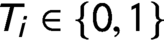 $T_i \in \{0, 1\}$
denotes the treatment received by unit i. For example,
 $T_i = 1$
would mean that unit i receives an informational message, and
 $T_i = 0$
would mean unit i is in a control group who does not receive any message. Based on the experimental design, treatment assignment probability
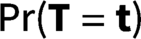 $\Pr (\mathbf {T}=\mathbf {t})$
is known for all
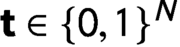 $\mathbf {t} \in \{0,1\}^N$
. Using the potential outcomes framework (Neyman Reference Neyman1923; Rubin Reference Rubin1974), let
 $Y_i (\mathbf {t})$
denote the potential outcome of individual i if the treatment assignment vector
 $\mathbf {T}$
is set to
 $\mathbf {t}$
. Importantly, the potential outcome of individual i is affected not only by her own treatment assignment, but also by the treatments received by others. Thus, we allow for spillover/interference between individuals (Cox Reference Cox1958; Rubin Reference Rubin1980). In our running example, voting behavior of a given individual can be affected not only by whether she directly receives the informational message, but also by messages assigned to her friends as people can share information with one another.
To formalize whose treatment status can affect a given individual, we rely on networks. In particular, consider two networks
 $\mathcal {G}$
and
 $\mathcal {U}$
connecting units with different edge sets. For example, people can be connected with Facebook and their offline face-to-face network. Formally, we define an adjacency matrix of network
 $\mathcal {G}$
to be
 $A^{\mathcal {G}}$
where
 $A^{\mathcal {G}}_{ij} = A^{\mathcal {G}}_{ji} = 1$
if unit i is connected to unit j (and zeros on the diagonal). We can also incorporate directed ties when we define
 $A^{\mathcal {G}}_{ij} = 1$
if unit i “follows” unit j, for example, on Twitter. By assigning different weights to each tie, this framework can accommodate the strength of ties as well. We then define individual i’s neighbors in network
 $\mathcal {G}$
to be other individuals to whom she is connected in network
 $\mathcal {G}$
, formally,
 $\mathcal {N}^{\mathcal {G}}_i \equiv \{j: A^{\mathcal {G}}_{ij} \neq 0\}.$
We define
 $A^{\mathcal {U}}$
and
 $\mathcal {N}^{\mathcal {U}}_i$
similarly. For example, neighbors are those with whom individual i is friends on Facebook (
 $\mathcal {N}^{\mathcal {G}}_i$
; neighbors on an online network) or those who individual i meets in person on a daily basis (
 $\mathcal {N}^{\mathcal {U}}_i$
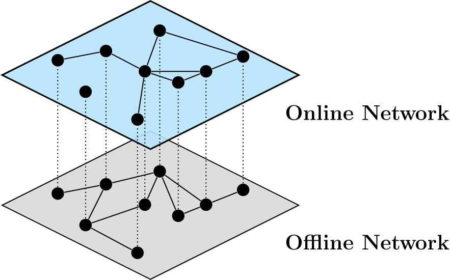
; neighbors on an offline face-to-face network). Importantly, neighbors in the two networks can overlap; we meet some but not all of our Facebook friends on a daily basis. Figure 1 visualizes an example with two networks.
Example of two networks. Note: The same set of people are connected differently by an online network and an offline network. Neighbors in the two networks overlap, i.e.,some, but not all, pairs of people are connected in both online and offline networks.

We explicitly incorporate these two networks into the potential outcomes. In particular, we extend the stratified interference assumption (Hudgens and Halloran Reference Hudgens and Halloran2008) to multiple networks. We assume that the potential outcomes of individual i are affected by her own treatment assignment and the treated proportions of neighbors in networks
 $\mathcal {G}$
and
 $\mathcal {U}$
(Manski Reference Manski2013; Toulis and Kao Reference Toulis and Kao2013; Liu and Hudgens Reference Liu and Hudgens2014; Forastiere et al.
Reference Forastiere, Airoldi and Mealli2016).
Assumption 1 Stratified Interference with Multiple Networks
For all
 $i,$
 $$ \begin{align*} Y_i (\mathbf{t}) = Y_i (d, g, u), \end{align*} $$
where d is her own treatment assignment, g and u are the proportions of treated neighbors in networks
 $\mathcal {G}$
and
 $\mathcal {U}$
, respectively:
 $$ \begin{align*} d & = t_i, \ \ g = \frac{\sum_{j \in \mathcal{N}_i^{\mathcal{G}}} t_j}{|\mathcal{N}_i^{\mathcal{G}}|}, \ \ u = \frac{\sum_{j \in \mathcal{N}_i^{\mathcal{U}}} t_j}{|\mathcal{N}_i^{\mathcal{U}}|}, \end{align*} $$
where
 $t_i$
is the treatment received by individual i.
 $\sum _{j \in \mathcal {N}_i^{\mathcal {G}}} t_j$
is the total number of treated units among individual i’s neighbors in network
 $\mathcal {G}$
and
 $|\mathcal {N}_i^{\mathcal {G}}|$
is the total number of individual i’s neighbors in network
 $\mathcal {G}$
.
 $\sum _{j \in \mathcal {N}_i^{\mathcal {U}}} t_j$
and
 $|\mathcal {N}_i^{\mathcal {U}}|$
are similarly defined.
The potential outcomes depend on the treatment assignment of herself d and the fractions of treated neighbors in each network
 $(g,u)$
. For example, the potential outcome of unit i is a function of whether she receives the informational message (d), the proportion of Facebook friends who receive the message (g), and the proportion of offline friends who receive the message (u). Although this assumption can only allow for spillover effects through treated proportions in multiple networks, it is more flexible than the conventional assumption of no interference, which requires that the treatment status of neighbors do not change potential outcomes at all. Formally, Assumption 1 can also be viewed as an exposure mapping
 $f(\mathbf {t}, (A^{\mathcal {G}}_{i}, A^{\mathcal {U}}_{i}))$
set to a three-dimensional vector
 $(d, g, u)$
(Aronow and Samii Reference Aronow and Samii2017).
Several points about Assumption 1 are worth clarifying. First, because this assumption is made at the individual level, an equivalent statement of Assumption 1 is that the potential outcomes depend on the treatment assignment of herself and the number (rather than proportions) of treated neighbors in each network. The only change is that when defining causal estimands, we should explicitly condition on the total number of neighbors in each network. Second, Assumption 1 is violated when neighbors in the same network have different spillover effects. For example, suppose a given individual i has three Facebook friends
 $\{F_1, F_2, F_3\}$
, and
 $F_1$
has a larger spillover effect than the other two. In this case, even when
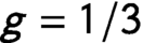 $g = 1/3$
, the potential outcomes of unit i differ depending on whether
 $F_1$
is treated or one of the other two is treated, which violates Assumption 1. Third and most importantly, unlike the previous literature, Assumption 1 is defined with multiple networks. Therefore, researchers can make the assumption more plausible by specifying networks more precisely. In the example above, suppose
 $F_1$
has a larger spillover effect than the other two because
 $F_1$
is also a friend of unit i on Twitter, whereas the other two are not. Then, we can restore Assumption 1 with respect to three networks; the Facebook network, the Twitter network, and an offline network. However, it is important to note that as we consider more networks, it is more difficult to observe all relevant networks, which is the central topic of the paper we further discuss in Sections 3 and 4.
We define networks to be causally relevant if treated proportions in such networks have nonzero causal effects.
Definition 1 Relevant Networks
Network
 $\mathcal {G}$
is causally relevant if
 $\ Y_i (d, g, u) \ \neq \ Y_i (d, g^\prime , u) $
for some i and
 $(d, g, u), (d, g^\prime , u) \in \Delta _i$
where
 $\Delta _i$
is the support of treatment exposure vector
 $(T_i, G_i, U_i)$
. The relevance of network
 $\mathcal {U}$
is similarly defined.
For example, if people do not talk about elections at all on Facebook, Facebook would be causally irrelevant because messages received by other Facebook friends would have no effect on voting behavior through Facebook when fixing treated proportions in the offline network.
Finally, as in the standard causal inference setting, we observe only one of many potential outcomes. For all i,
 $ Y_i = \sum _{(d,g,u) \in \Delta _i} \mathbf {1}\{T_i=d, G_i=g, U_i=u\} \ Y_i(d,g,u)$
(Holland Reference Holland1986).
2.2 Causal Quantities of Interest
Without loss of generality, we assume two networks
 $\mathcal {G}$
and
 $\mathcal {U}$
are causally relevant and define our quantities of interest using these two networks.
2.2.1 Direct Effects and Network-Specific Spillover Effects
First, we define the direct effect of a treatment. It is the difference between the potential outcomes under treatment and control, averaging over the distribution of treatment assignment
 $(G_i, U_i)$
. Formally, we define the average direct effect (ADE) as follows.
Definition 2 Average Direct Effect
 $$ \begin{align} \delta \ \equiv \ \frac{1}{N} \sum_{i=1}^N \left\{\sum_{(g,u) \in \Delta_i^{gu}} \{Y_i(1, g, u) - Y_i(0, g, u)\} \Pr(G_i=g, U_i=u)\right\}, \end{align} $$
where the support is defined as
 $\Delta _i^{gu} = \{(g,u):\Pr (G_i=g, U_i=u)> 0\}.$
It is the weighted average of the causal effects,
 $Y_i(1, g, u) - Y_i(0, g,u)$
, which hold the proportions of treated neighbors in the two networks constant. Intuitively, this effect quantifies the causal impact of the treatment directly received by herself. Thus, the ADE could represent the direct causal effect of the informational message on voting behavior. The ADE is a simple extension of the expected average treatment effect (Sävje et al.
Reference Sävje, Aronow and Hudgens2017) to the two-network settings. We keep the term of the direct effect in order to distinguish it from spillover effects we define next.
Spillover effects describe the causal effects of the neighbors’ treatment status on a given individual. It is the change in the potential outcome when the proportion of treated neighbors goes from a lower proportion to a higher proportion. Formally, it is the difference between the potential outcome for a given individual when
 $g^H \times 100\%$
of her neighbors in
 $\mathcal {G}$
are treated and the other potential outcome for the same individual when
 $g^L \times 100\%$
of her neighbors in
 $\mathcal {G}$
are treated, holding her own treatment assignment and averaging over the proportions of treated neighbors in
 $\mathcal {U}$
. Two constants
 $g^H$
and
 $g^L$
stand for “Higher” and “Lower” percent. We define the average network-specific effect (ANSE) as follows.
Definition 3 Average Network-Specific Spillover Effect
 $$ \begin{align} \tau (g^H, g^L ; d) \ \equiv \ \frac{1}{N} \sum_{i=1}^N \left\{\sum_{u \in \Delta_i^u} \{Y_i(d, g^H, u) - Y_i(d, g^L, u) \} \ \Pr (U_i=u \mid T_i=d, G_i = g^L)\right\}, \end{align} $$
where the support is defined as
 $\Delta _i^{u} = \{u: \Pr (U_i=u \mid T_i=d, G_i = g^H)> 0 \mbox { and } \Pr (U_i=u \mid T_i=d, G_i = g^L) > 0\}.$
The ANSE for network
 $\mathcal {U}$
is defined similarly.
It is the weighted average of the spillover effects specific to network
 $\mathcal {G}$
,
 $Y_i(d, g^H, u) - Y_i(d, g^L,u)$
, which hold her own treatment assignment and the proportion of treated neighbors in
 $\mathcal {U}$
constant. Thus, for example, the ANSE
 $(g^H=0.8, g^L=0.2; d = 0)$
could represent the Facebook-specific spillover effect where we change the treated proportion of one’s Facebook friends (from
 $g^L = 20$
% to
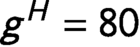 $g^H = 80$
%) while holding constant one’s own treatment assignment (
 $d = 0$
) and averaging over the treated proportion of one’s offline friends (u). Similarly, the ANSE
 $(u^H =0.8, u^L=0.2; d = 0)$
could represent the offline network-specific spillover effect where we change the treated proportion of one’s offline friends (from
 $u^L = 20$
% to
 $u^H = 80$
%) while holding constant one’s own treatment assignment (
 $d = 0$
) and averaging over the treated proportion of one’s Facebook friends (u).
Importantly, the ANSE captures the spillover effect specific to each network separately. Thus, when Facebook (the offline network) is causally irrelevant, as defined in Definition 1, the ANSE in Facebook (the offline network) will be zero. By estimating the ANSE for each network, researchers can unpack the mechanism of spillover effects; which networks do people use to share information and influence each other’s voting behavior? In Appendix B, we additionally show that the ANSE decomposes the total spillover effect, a popular estimand in the literature (Hudgens and Halloran Reference Hudgens and Halloran2008), into each network.
2.3 Estimation
In this section, we study the estimation of the ADE and the ANSE. We begin by introducing a common assumption made in practice; the no omitted network assumption defined below.
Assumption 2 No Omitted Network
All causally relevant networks are observed.
For example, in the Facebook mobilization experiment (Bond et al. Reference Bond2012), this assumption of no omitted network means that the Facebook network is the only relevant network and an unobserved face-to-face network is irrelevant; experimental subjects could affect one another through Facebook but not through their unobserved offline interactions. We first examine the estimation under this assumption and then discuss its violation in the subsequent sections.
Following the recent literature (e.g., Hudgens and Halloran Reference Hudgens and Halloran2008; Tchetgen Tchetgen and VanderWeele Reference Tchetgen Tchetgen and VanderWeele2010; Kang and Imbens Reference Kang and Imbens2016; Sussman and Airoldi Reference Sussman and Airoldi2017), we start with design-based, inverse probability weighting (IPW) estimators for the ADE and ANSE (Horvitz and Thompson Reference Horvitz and Thompson1952; Aronow and Samii Reference Aronow and Samii2017). Importantly, researchers can compute the treatment exposure probability
 $\Pr (T_i = d, G_i = g, U_i = u)$
from the experimental design under the no omitted network assumption.Footnote
1
Thus, we rely on the following weighting estimators.
Theorem 1 Estimation of the ADE and the ANSE
Under Assumption 2, the treatment exposure probability
 $\Pr (T_i=d, G_i=g, U_i=u)$
is known for all
 $(d, g, u) \in \Delta _i$
and all i. Therefore, the average direct effect and the average network-specific spillover effect in
 $\mathcal {G}$
can be estimated by the following inverse probability weighting estimators.
 $$ \begin{align*} \mathbb{E}[\hat{\delta}] = \delta \quad \text{and} \quad \mathbb{E}[\hat{\tau}(g^H, g^L; d) ] = \tau(g^H, g^L; d), \end{align*} $$
where the expectation is taken over the experimental design
 $\Pr (\mathbf {T}=\mathbf {t})$
, and
 $$ \begin{align} \hat{\delta} &\equiv \frac{1}{N} \sum_{i=1}^N \mathbf{1}\{T_i=1\} \tilde{w}_i Y_i - \frac{1}{N} \sum_{i=1}^N \mathbf{1}\{T_i=0\} \tilde{w}_i Y_i \end{align} $$
 $$ \begin{align} \hat{\tau}(g^H, g^L; d) & \equiv \frac{1}{N} \sum_{i=1}^N \mathbf{1}\{T_i = d, G_i = g^H\} w_i Y_i - \frac{1}{N} \sum_{i=1}^N \mathbf{1}\{T_i = d, G_i = g^L\} w_i Y_i, \end{align} $$
and weights are defined as
 $$ \begin{align*} \tilde{w}_i = \frac{1}{\Pr(T_i \mid G_i, U_i)}, \quad \text{and} \quad w_i = \frac{\Pr(U_i \mid T_i, G_i = g^L)}{\Pr(U_i \mid T_i, G_i)} \times \frac{1}{\Pr(T_i, G_i)}. \end{align*} $$
We provide the proof in Appendix C.1. Although the IPW estimators are unbiased, researchers might want to increase efficiency by incorporating covariate information and some parametric assumptions (Särndal et al. Reference Särndal, Swensson and Wretman1992). In particular, we build on the design-based IPW estimator above and propose a weighted linear regression estimator. This alternative approach reduces standard errors at the expense of some bias due to parametric modeling assumptions. In particular, we consider
 $$ \begin{align} Y_i \sim \alpha + \beta T_i + \gamma_0 G_i + \gamma_1 (T_i \times G_i) + \mathbf{X}^\top_ i \theta \mbox{ with weights } w_i. \end{align} $$
The key assumptions are the linearity of
 $G_i$
and the inclusion of pretreatment covariates
 $\mathbf {X}_i$
.Footnote
2
We emphasize an important tradeoff. On the one hand, both assumptions are parametric in the sense that they are not directly justified by the experimental design. On the other hand, they tend to greatly reduce variance. Especially in settings with multiple networks, treatment exposure probabilities
 $\Pr (T_i, G_i, U_i)$
are usually small, and in many applied contexts, the standard IPW estimator has large standard errors. The weighted linear regression estimator aims to balance this bias-variance tradeoff in practice. See Toulis and Kao (Reference Toulis and Kao2013) for a Bayesian approach, and Särndal et al.(Reference Särndal, Swensson and Wretman1992); Rosenbaum (Reference Rosenbaum2002) and Aronow and Samii (Reference Aronow and Samii2017) for the design-based covariate adjustment.
3 Exact Bias Formula
We can obtain an unbiased estimate of the ANSE when we observe all relevant networks. However, this assumption of no omitted network is often violated in practice, and if so, the ANSE even in the observed network cannot be estimated without bias. For example, in Bond et al.(Reference Bond2012), while the Facebook network is observed, an offline face-to-face network is unobserved. In this case, even with randomized experiments, an estimate of the Facebook-specific spillover effect is biased because people can potentially share information with offline friends. Bond et al.(Reference Bond2012) write, “it is plausible that unobserved face-to-face interactions account for at least some of the social influence that we observed in this experiment” (p. 298). In this section, to explicitly characterize sources of such bias, we derive the exact bias formula for the ANSE. We provide the exact bias formula for the ADE in Appendix C.2.1.
We consider a common research setting in which the main network of interest is observed but other relevant networks are not observed. In particular, we assume
 $\mathcal {G}$
is an observed network of interest and
 $\mathcal {U}$
is unobserved.Footnote
3
Thus, the quantity of interest is the ANSE in the observed network
 $\mathcal {G}$
. For simplicity, we refer to the ANSE in
 $\mathcal {G}$
as the ANSE, without explicitly mentioning
 $\mathcal {G}$
.
Since network
 $\mathcal {U}$
is unmeasured, we cannot use weights
 $w_i$
discussed in Section 2.3. Instead, we can only rely on partial weights
 $ w^{\mathtt {B}}_i \equiv 1/\Pr (T_i, G_i)$
where we only adjust for the direct treatment assignment
 $T_i$
and the treated proportion in the observed network
 $G_i$
. For example, the IPW estimator based on such partial weights becomes
 $$ \begin{align} \frac{1}{N} \sum_{i=1}^N \biggl\{ \mathbf{1}\{T_i=d, G_i=g^H\}w_i^{\mathtt{B}} Y_i - \mathbf{1}\{T_i=d, G_i=g^L\}w_i^{\mathtt{B}} Y_i\biggr\}. \end{align} $$
We use
 $\hat {\tau }_B (g^H, g^L; d)$
to denote any estimator with partial weights
 $w^{\mathtt {B}}_i$
, including both the IPW estimator and the regression estimator discussed in Section 2.3. For the regression estimator, the bias formula we derive next can be seen as the lower bound where we focus only on the bias due to unobserved networks and not on bias due to functional form assumptions.
The next theorem shows the exact bias formula for
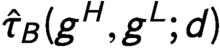 $\hat {\tau }_B (g^H, g^L; d)$
in settings where the no omitted network assumption does not hold.
Theorem 2 Bias for the ANSE due to Omitted Networks
When the no omitted network assumption (Assumption 2) is violated, estimator
 $\hat {\tau }_B (g^H, g^L; d)$
is biased for the ANSE.
 $$ \begin{align*} & \mathbb{E}[\hat{\tau}_B (g^H, g^L; d)] - \tau (g^H, g^L; d)\\[5pt] & = \frac{1}{N} \sum_{i=1}^N \biggl\{ \sum_{u \in \Delta_i^u} \{Y_i (d, g^H, u) - Y_i(d, g^H, u^\prime)\} \{ \Pr(U_i=u|T_i=d, G_i=g^H) - \Pr(U_i=u|T_i=d, G_i = g^L)\}\biggr\}, \end{align*} $$
for any
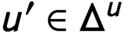 $u^\prime \in \Delta ^u$
.
We provide the proof in Appendix C.2. This bias can be decomposed into two parts: (1) the spillover effects attributable to the unobserved network
 $\mathcal {U}$
,
 $Y_i (d, g^H, u) - Y_i(d, g^H, u^\prime )$
and (2) the dependence between the fraction of treated neighbors in
 $\mathcal {G}$
and the fraction of treated neighbors in
 $\mathcal {U}$
,
 $\Pr (U_i=u \mid T_i=d, G_i=g^H) - \Pr (U_i=u \mid T_i=d, G_i = g^L)$
.
Based on this decomposition, we offer several implications of the theorem. First, when treatment assignment to
 $\mathcal {U}$
has no effect (i.e.,
 $\mathcal {U}$
is irrelevant),
 $Y_i (d, g^H, u) - Y_i(d, g^H, u^\prime ) \ = \ 0$
for any i. In this simple case, the bias is zero; this formula includes the assumption of no omitted network as a special case.
Second, the dependence between the fraction of treated neighbors in
 $\mathcal {G}$
and the fraction of treated neighbors in
 $\mathcal {U}$
determines the size and sign of the bias. In theory, when
 $G_i$
and
 $U_i$
are independent given
 $T_i$
, the bias is zero. However,
 $G_i$
and
 $U_i$
are in general dependent given
 $T_i$
. Two points about this dependence are worth noting. First, some randomization of treatment assignment, such as a Bernoulli design, can make
 $T_i$
independent of
 $(G_i, U_i)$
, but
 $G_i$
and
 $U_i$
are dependent given
 $T_i$
even after any randomization of treatment assignment because some neighbors in
 $\mathcal {G}$
are also neighbors in the other network
 $\mathcal {U}$
; networks
 $\mathcal {G}$
and
 $\mathcal {U}$
overlap each other. Formally,
 $G_i$
and
 $U_i$
are dependent because both are functions of the treatment assignment to common neighbors. Second, based on the same logic,
 $G_i$
and
 $U_i$
are not independent given
 $T_i$
even when two networks
 $\mathcal {G}$
and
 $\mathcal {U}$
are independently generated because the two networks can still overlap each other.
For example, the Facebook network and an unobserved face-to-face network are likely to overlap each other. For some users, their Facebook friends are also close friends to whom they have offline interactions and vice versa. As long as the spillover effects in the face-to-face network are non-zero, an estimator ignoring this unobserved offline network (Equation (6)) would be biased for the Facebook-specific spillover effect.
Finally, we illustrate the bias with a simple linear model,
 $ Y_i (T_i, G_i, U_i) \ = \alpha + \beta T_i + \gamma G_i + \lambda U_i + \epsilon _i$
where
 $\epsilon _i$
is an error term. Under the model, the potential outcome of individual i depends on neighbors in both
 $\mathcal {G}$
and
 $\mathcal {U}$
, and such two network-specific spillover effects do not interact. In this simple setup, the bias can be simplified as follows.
 $$ \begin{align*} \mathbb{E}[\hat{\tau}_B(g^H, g^L; d)] - \tau(g^H,g^L; d) &= \lambda \times \frac{1}{N} \sum_{i=1}^N \{\mathbb{E}[U_i \mid T_i=d, G_i=g^H] - \mathbb{E}[U_i \mid T_i=d, G_i=g^L]\}. \end{align*} $$
It is clear that the bias depends on the ANSE in the unobserved network
 $\mathcal {U}$
(i.e.,
 $\lambda $
) and the association between
 $U_i$
and
 $G_i$
given
 $T_i$
. This bias is not zero unless the unobserved network
 $\mathcal {U}$
is irrelevant because
 $\mathbb {E}[U_i \mid T_i=d, G_i=g^H] \ \neq \ \mathbb {E}[U_i \mid T_i=d, G_i=g^L]$
in general.
4 Sensitivity Analysis
We address the potential violation of the no omitted network assumption by developing parametric and nonparametric sensitivity analysis methods for the ANSE.
4.1 Parametric Sensitivity Analysis
Although the exact bias formula in Theorem 2 does not make any assumption about the unobserved network
 $\mathcal {U}$
, in order to use it in applied work, it requires specifying a large number of sensitivity parameters. To construct a practical parametric sensitivity analysis method, we rely on a simplifying parametric assumption. In particular, we consider the assumption that the network-specific spillover effect in an unobserved network is linear and additive (Sussman and Airoldi Reference Sussman and Airoldi2017).
Assumption 3 Linear, Additive Network-Specific Spillover Effect in
 $\mathcal {U}$

 $$ \begin{align*} \frac{1}{\sum_{i=1}^N \mathbf{1}\{S_i=s\}}\sum_{i:S_i=s} \{Y_i(d, g, u) - Y_i(d, g, u^\prime)\} = \lambda (u- u^\prime), \end{align*} $$
with some coefficient
 $\lambda $
for all
 $(d, g, u), (d, g, u^\prime ) \in \Delta _s$
where
 $\Delta _s$
is the support of
 $(d, g, u)$
for i with the neighbors’ profile
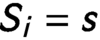 $S_i=s$
. The neighbors’ profile S is defined such that the probability of treatment exposure is the same for those who have the same neighbors’ profile. Formally, for
 $i \neq j$
,
 $\Pr (T_i=d, G_i=g, U_i=u) = \Pr (T_j=d, G_j=g, U_j=u)$
when
 $S_i=S_j.$
For example, when the Bernoulli or completely randomized design is used,
 $S_i$
is simply a vector of three values; the number of neighbors in
 $\mathcal {G}$
and
 $\mathcal {U}$
, and the number of neighbors common to the two networks.
While this linear additive assumption is strong, it is commonly used in the causal inference literature to derive intuitive, easy-to-use sensitivity analysis methods. For example, the widely used sensitivity analysis methods for unobserved confounders in observational studies rely on similar assumptions (VanderWeele and Arah Reference VanderWeele and Arah2011). We also consider nonparametric sensitivity analysis in the next section under weaker assumptions.
Under Assumption 3, the general bias formula becomes the multiplication of two terms: the network-specific spillover effect in
 $\mathcal {U}$
, that is,
 $\lambda $
, and the effect of
 $G_i$
on
 $U_i$
given
 $T_i$
, that is,
 $ \frac {1}{N} \sum _{i=1}^N \{ \mathbb {E}[U_i \mid T_i=d, G_i=g^H] - \mathbb {E}[U_i \mid T_i=d, G_i=g^L] \}.$
The following theorem shows a simplified bias formula for settings with sparse
 $\mathcal {G}$
.
Theorem 3 Parametric Sensitivity Analysis
Under Assumption 3, a bias formula is approximated as follows.
 $$ \begin{align} \mathbb{E}[\hat{\tau}_B (g^H, g^L; d)] - \tau (g^H, g^L; d) \approx \lambda \times \pi_{GU} \times (g^H - g^L), \end{align} $$
where
 $\lambda $
is the ANSE in network
 $\mathcal {U}$
and
 $\pi _{GU}$
is the overlap, that is, the fraction of neighbors in
 $\mathcal {U}$
who are also neighbors in
 $\mathcal {G}$
. Formally,
 $\pi _{GU} \equiv \sum _{i=1}^N \{|\mathcal {N}^{(\mathcal {G},\mathcal {U})}_i| / |\mathcal {N}^{\mathcal {U}}_i|\}/N$
where
 $|\mathcal {N}^{(\mathcal {G},\mathcal {U})}_i|$
is the number of unit i’s neighbors common to the two networks. If an experiment uses a Bernoulli design, the approximation is exact regardless of the sparsity of network
 $\mathcal {G}.$
We provide the proof in Appendix C.3. This simplified bias formula offers several implications. First, the bias is small when
 $\pi _{GU}$
is small, that is, the overlap of neighbors in
 $\mathcal {G}$
and
 $\mathcal {U}$
is small. Hence, the bias is close to zero when the network
 $\mathcal {G}$
is sparse and neighbors in
 $\mathcal {G}$
and
 $\mathcal {U}$
are disjoint. Second, even if two networks
 $\mathcal {G}$
and
 $\mathcal {U}$
are independently generated, the bias is not zero because
 $\pi _{GU} \neq 0$
. We derive a similar parametric bias formula for settings with nonsparse
 $\mathcal {G}$
in Appendix C.3.
For example, the overlap between the Facebook network and the unobserved face-to-face network is defined to be the fraction of offline friends who are also friends on Facebook. When this overlap is large (small), we expect the bias for the Facebook-specific spillover effect to be large (small).
To use this formula for a sensitivity analysis, researchers need to specify two sensitivity parameters: the network-specific spillover effect in an unobserved network (i.e.,
 $\lambda $
) and the fraction of neighbors in
 $\mathcal {U}$
who are also neighbors in
 $\mathcal {G} $
(i.e.,
 $\pi _{GU}$
). Once these two parameters are specified, we can derive the bias. Subsequently, because the bias utilizes only sensitivity parameters and
 $(g^H - g^L)$
, we can obtain a bias corrected estimate by subtracting this bias from
 $\hat {\tau }_B (g^H, g^L; d)$
. A sensitivity analysis is to report the estimated ANSE under a range of plausible values of
 $\lambda $
and
 $\pi _{GU}$
where
 $0 < \pi _{GU} < 1.$
Note that
 $\lambda = 0 $
corresponds to the no omitted network assumption.
4.2 Nonparametric Sensitivity Analysis
Now, we provide a nonparametric sensitivity analysis that makes only one assumption of non-negative outcomes. While we introduce our method using a random variable
 $U_i$
for simplicity, the same method can be applied to a random vector
 ${\mathbf { U_i}}$
and accommodate multiple unobserved networks. The proposed method is an extension of a sensitivity analysis developed for observational studies with no spillover effect (Ding and VanderWeele Reference Ding and VanderWeele2016) to experimental settings where spillover effects in unobserved networks induce bias.
As the parametric sensitivity analysis, we use two sensitivity parameters: intuitively, the network-specific spillover effect in
 $\mathcal {U}$
, and the association between
 $U_i$
and
 $G_i$
. To capture the network-specific spillover effect in
 $\mathcal {U}$
, let
 $\mathrm {MR}_{UY} (g, s)\equiv \max\nolimits_{u} \sum _{i; S_i=s} Y_i(d, g, u) / \min\nolimits_{u}\sum _{i;S_i=s} Y_i (d,g,u)$
denote the largest potential outcomes ratios of
 $U_i$
on
 $Y_i$
given
 $T_i=d, G_i=g$
and
 $S_i=s$
. For notational simplicity, we drop subscript d whenever it is obvious from contexts. Then, we define
 $\mathrm {MR}_{UY} = \max\nolimits_{g \in (g^H, g^L), \ s \in \mathcal {S}} \ \mathrm {MR}_{UY} (g, s)$
as the largest potential outcomes ratio of
 $U_i$
on
 $Y_i$
over
 $g \in \{g^H, g^L\}$
and
 $s \in \mathcal {S}.$
Thus,
 $\mathrm {MR}_{UY}$
quantifies the largest possible potential outcomes ratio of
 $U_i$
on
 $Y_i$
. This ratio captures the magnitude of the network-specific spillover effect in
 $\mathcal {U}$
. When network
 $\mathcal {U}$
is irrelevant,
 $\mathrm {MR}_{UY} = 1$
.
Furthermore, to quantify the association between
 $G_i$
and
 $U_i$
, we use
 $\mathrm {RR}_{GU} (g, g^\prime ,u, s) \ = \ \Pr (U_i=u \mid T_i=d, G_i=g) \ / \ \Pr (U_i=u \mid T_i=d, G_i=g^\prime )$
to denote the relative risks of
 $G_i$
on
 $U_i$
for all i with
 $S_i=s$
.
 $ \mathrm {RR}_{GU} \ = \ \max\nolimits_{(g, g^\prime ) \in (g^H, g^L), u \in \Delta ^u, s \in \mathcal {S}} \ \mathrm {RR}_{GU} (g, g^\prime ,u, s)$
is the maximum of these relative risks. This risk ratio captures the association between
 $G_i$
and
 $U_i$
.
Using these ratios, we can derive an inequality that the ANSE in the observed network
 $\mathcal {G}$
needs to satisfy as long as outcomes are non-negative. The next theorem shows that we can obtain the bound for the ANSE with two sensitivity parameters,
 $\mathrm {MR}_{UY}$
and
 $\mathrm {RR}_{GU}$
.
Theorem 4 Bound on the ANSE
When outcomes are non-negative,
 $$ \begin{align*} & \mathbb{E}\biggl[ \frac{\hat{m}(d, g^H)}{B} - B \hat{m}(d, g^L) \biggr] \ \leq \ \tau (g^H, g^L; d) \ \leq \ \mathbb{E}\biggl[ B \hat{m}(d, g^H) - \frac{\hat{m}(d, g^L)}{B} \biggr], \end{align*} $$
where
 $B = (\mathrm {RR}_{GU} \times \mathrm {MR}_{UY})/ (\mathrm {RR}_{GU} + \mathrm {MR}_{UY} - 1)$
and
 $\hat {m}(d, g) = \frac {1}{N} \sum _{i=1}^N \mathbf {1}\{T_i=d, G_i=g\} w_i^{\mathtt {B}}Y_i$
for
 $g \in \{g^H, g^L\}$
.
We provide the proof in Appendix C.4. Note that
 $\mathrm {MR}_{UY} = 1 $
corresponds to the no omitted network assumption, and
 $\mathbb {E}[\hat {m}(d, g^H) - \hat {m}(d, g^L)] = \mathbb {E}[\hat {\tau }_B (g^H, g^L; d)] = \tau (g^H, g^L; d)$
under the assumption. B is an increasing function of both
 $\mathrm {RR}_{GU}$
and
 $\mathrm {MR}_{UY}$
, implying that the bound is wider when the network-specific spillover effect in the unobserved network
 $\mathcal {U}$
is larger and the effect of
 $G_i$
on the distribution of
 $U_i$
is larger. In fact, the size of the bound is given by
 $(B - \frac {1}{B}) \mathbb {E}[\hat {m}(d, g^H) + \hat {m}(d, g^L)].$
It is important to note that the bound is not location-invariant because we use mean ratios and risk ratios as sensitivity parameters (Ding and VanderWeele Reference Ding and VanderWeele2016). The bound is valid as far as outcomes are non-negative, but how informative it is can vary. To conduct the sensitivity analysis, one can compute the bound for a range of plausible values of
 $\mathrm {MR}_{UY}$
and
 $\mathrm {RR}_{GU}$
. Compared to the parametric sensitivity analysis,
 $\mathrm {MR}_{UY}$
and
 $\mathrm {RR}_{GU}$
correspond to
 $\lambda $
and
 $\pi _{GU},$
respectively. Finally, as in Section 2.3, we can also use a weighted linear regression estimator for
 $\hat {m}(d, g)$
instead of the IPW estimator.
5 Simulation Study: Twitter Mobilization Experiment
Based on the real-world Twitter network (Coppock et al. Reference Coppock, Guess and Ternovski2016), we conduct a simulation study where we generate a variety of unobserved offline face-to-face networks. We evaluate how well the sensitivity analysis methods estimate the Twitter-specific spillover effect.
We vary the simulation setup along two dimensions; (1) the overlap between the observed Twitter network and a simulated unobserved offline network and (2) the outcome data generating process—a linear additive model or an interactive model. With this design, we illustrate three key results we derived analytically. First, the bias increases when the overlap between the online network and the unobserved offline network increases (Theorem 2). Second, the parametric sensitivity analysis can recover unbiased estimates under a linear additive model but suffers from bias under an interactive model (Theorem 3). Finally, the nonparametric sensitivity analysis provides bounds for the ANSE under both models, but it has larger confidence intervals than the parametric version under the linear additive model (Theorem 4).
Background
To make our simulation as realistic as possible, we rely on the real-world Twitter network studied in Coppock et al.(Reference Coppock, Guess and Ternovski2016). The original authors conducted a political mobilization experiment over the Twitter network to estimate the effectiveness of online mobilization appeals. In particular, they sampled followers of the Twitter account of a nonprofit advocacy organization, the League of Conservation Voters (LCV), and measured a network adjacency matrix among them. Each node of the network is a Twitter user who follows the LCV’s account and a directed edge exists from user i to user j when user i follows user j. Instead of artificial simulated networks, we use this real-world Twitter network as the basis of our simulations after preprocessing as described below.
Simulation design
To make the comparison of sensitivity analysis methods clear, we preprocess the Twitter network of Coppock et al.(Reference Coppock, Guess and Ternovski2016). First, to avoid the influence of outliers, we remove units that are above the 95th percentile of the distribution on the size of Twitter neighbors (also known as the out-degree distribution). To have well-defined treated proportions
 $G_i$
(explain more below), we also remove those who follow less than five other units. The resulting network contains
 $2,430$
units with the mean number of neighbors equal to
 $18.5$
. We simulate an unobserved offline network
 $\mathcal {U}$
with four different values of the overlap
 $\pi _{GU}\in \{0.0, 0.2, 0.4, 0.6\}$
where we expect no bias in the case of
 $\pi _{GU} = 0$
. We use the Bernoulli design to randomly assign treatments with probability
 $0.5.$
We consider two outcome data generating processes. For the linear additive model, we generate potential outcomes for individual i by
 $ Y_i (T_i, G_i, U_i) \ = 5 + 2 T_i + G_i + 1.5 U_i + \epsilon _i,$
where
 $\epsilon _i$
is randomly drawn from a normal distribution with
 $(\mu , \sigma ) = (0.0, 0.5)$
.
 $G_i$
and
 $U_i$
denote treated proportions of neighbors in the observed Twitter network and unobserved treated proportions of neighbors in the offline network, respectively. For the interactive model, we use
 $ Y_i (T_i, G_i, U_i) \ = 5 + 2 T_i + G_i + 2 T_i \times U_i + 2 G_i \times U_i + 0.5 U_i + \epsilon _i$
. As the main causal estimand, we consider the ANSE,
 $\tau (0.6, 0.4; 0)$
, where we compare
 $g^H=0.6$
relative to
 $g^L=0.4$
when
 $d=0$
(to have
 $G_i = 0.6$
and
 $G_i= 0.4$
both well-defined, we focus on a subset of units who follows at least five units). In the linear additive model, the true ANSE is equal to
 $0.2$
, and in the interactive model, the true ANSE is approximately equal to
 $0.4$
(the exact values change according to the overlap
 $\pi _{GU}$
).
The offline network
 $\mathcal {U}$
is unmeasured and thus, we can rely only on a linear regression
 $Y_i \sim \alpha + \beta T_i + \gamma _0 G_i + \gamma _1 (T_i \times G_i)$
with weights
 $w_i^{\mathtt {B}} = 1/\Pr (T_i, G_i).$
An estimator,
 $0.2 \times \hat {\gamma }_0,$
is biased for
 $\tau (0.6, 0.4; 0)$
due to unobserved network
 $\mathcal {U}.$
The parametric sensitivity analysis provides a bias-corrected estimate,
 $0.2 \times \hat {\gamma }_0 - 0.2 \times \lambda \times \pi _{GU},$
with two sensitivity parameters; the overlap
 $\pi _{GU}$
and the spillover effect in the unobserved network
 $\lambda $
.Footnote
4
The nonparametric sensitivity analysis computes bounds with sensitivity parameters
 $(\mathrm {MR}_{UY}, \mathrm {RR}_{GU})$
.Footnote
5
We evaluate an estimator that ignores unobserved offline networks, the parametric sensitivity analysis, and the nonparametric sensitivity analysis with the
 $2,000$
Monte Carlo simulations.
Results
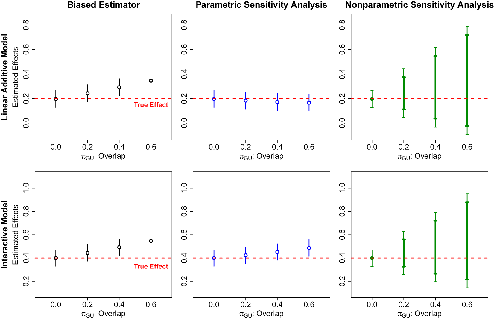
Figure 2 presents simulation results. The first column reports estimates,
 $0.2 \times \hat {\gamma }_0,$
that ignore the unobserved network
 $\mathcal {U}$
, with the 95% confidence intervals (CI). Both settings of the linear additive and interactive models illustrate that the estimator is biased unless the overlap
 $\pi _{GU}$
is zero, and the bias increases as the overlap increases. The second column shows the results for the parametric sensitivity analysis with the 95% CI. In the linear additive model setup (the first row), the parametric sensitivity analysis recovers approximately unbiased estimates. In contrast, in the interactive model setup (the second row), it still suffers from bias as the linear additive assumption (Assumption 3) is violated. Finally, the third column reports bounds from the nonparametric sensitivity analysis (thick bars) and the 95% CI of the bounds (thin bars). When the overlap
 $\pi _{GU}$
is zero, the bound converges to an unbiased point estimate of the ANSE. Importantly, the bounds cover the true ANSE in both linear additive and interactive model settings as Theorem 4 implies. It also reveals an important limitation; while the nonparametric bounds cover the true ANSE, they are much wider than the 95% CI of the parametric sensitivity analysis under the linear additive model. This is the case especially when the overlap between the main network of interest and the unobserved network is large.
Simulation results on bias and sensitivity analysis for the Twitter experiment. Note: The first (second) row reports results from the linear additive (interactive) model. The first column demonstrates the bias in estimators that ignore the unobserved offline network. The second column shows that the parametric sensitivity analysis can recover unbiased estimates of the ANSE under the linear additive model but not under the interactive model. The third column demonstrates that bounds from the nonparametric sensitivity analysis cover the true ANSE, but are much wider than the parametric version under the linear additive model.

6 Empirical Application: Network Field Experiment
Cai et al.(Reference Cai, De Janvry and Sadoulet2015) are interested in understanding how farmers in rural China use social networks to make important financial decisions, that is, insurance take-up. They designed an experiment with China’s largest insurance provider, the People’s Insurance Company of China (PICC), to randomly assign households to different information sessions about the insurance. While they estimate the direct treatment effect as a first step, the primary focus of the original analysis is to estimate the spillover effect of such information on the insurance take-up.
As in many other network field experiments, they use a social network survey to ask experimental subjects to name their network connections. In particular, they asked household heads to name five close friends with whom “they most frequently discuss rice production or financial issues” (Cai et al.
Reference Cai, De Janvry and Sadoulet2015, p. 88). Although this is a popular strategy, there are several reasons to afraid of unobserved networks. First, as carefully noted in the original paper, almost all households listed the maximum number of friends (the average number of listed friends is
 $4.9$
where respondents can only list up to
 $5$
friends), which suggests that respondents could have listed more friends if other forms of network surveys were used (Larson and Lewis Reference Larson and Lewis2020). Second, networks among experimental subjects are dense; “the average path-length is about
 $2.67$
, which means that a household can be connected to any other household in the village by passing on average of two to three households” (Cai et al.
Reference Cai, De Janvry and Sadoulet2015, p. 89). This suggests that there are many potential network connections through which experimental subjects can communicate with each other. For example, in such rural Chinese villages, a kinship network is of great importance (e.g., Xiong and Payne Reference Xiong and Payne2017).
We extend the original analysis by estimating the spillover effect specific to the observed financial network while accounting for unobserved networks, such as the kinship network.
Setup
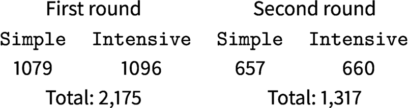
Cai et al.(Reference Cai, De Janvry and Sadoulet2015) designed the experiment with two rounds to estimate the spillover effect. A total of 2,175 households were invited to the first round and they were randomly assigned into one of two information sessions, simple or intensive. The simple session took about 20 min and the PICC agents explained the insurance contract. The intensive sessions took about 45 min and provided all the information given in the simple session, plus an additional detailed explanation of expected benefits and costs of purchasing the insurance. Three days after the first round, a different set of households were invited to the second round and randomly assigned into the simple or intensive sessions. We follow the original analysis and focus on 1,317 households who were invited to this second round and only received information from the simple or intensive session (657 and 660 households, respectively).Footnote 6 The main outcome of interest is a binary variable whether each household in the second round takes up the insurance. Table 1 summarizes the relevant aspects of the experimental design. See Cai et al.(Reference Cai, De Janvry and Sadoulet2015) for details and other features of the design.
Experimental design.

For participants in the second round, the original authors define the main exposure variable of interest
 $G_i$
to be the proportion of peers in their financial network who attended the first round intensive session. The direct treatment
 $T_i$
is defined as an indicator variable taking
 $1$
if household i receives the intensive session and
 $0$
otherwise. Following their analysis, we focus on the ANSE specific to the observed financial network and compare
 $g^H = 0.2$
and
 $g^L = 0$
under no direct treatment receipt
 $d= 0$
, formally
 $\tau (g^H = 0.2, g^L = 0; d = 0)$
, as they show the biggest difference is between no treated peer and one treated peer (table 3 of the original paper). In addition, to satisfy the standard overlap assumption (Imbens and Rubin Reference Imbens and Rubin2015), we analyze units who listed the maximum number of five householdsFootnote
7
in the financial network question (1,207 households, more than 90% of all the samples).
To estimate spillover effects, the original authors estimate the following linear regression (model 4 in table 2 of Cai et al.(Reference Cai, De Janvry and Sadoulet2015)) with standard errors clustered at the village level.
 $$ \begin{align} Y_i = \alpha + \beta T_i + \gamma_0 G_i + \gamma_1 (T_i \times G_i) + \mathbf{X}^\top_i \theta + \epsilon_i, \end{align} $$
where pretreatment covariates
 $\mathbf {X}_i$
include the size of neighbors, village fixed effects, and other household characteristics (gender, age, education of household head, rice production area, risk aversion, and perceived probability of future disaster). Thus, if the observed financial network is the only causally relevant network (i.e., the no omitted network assumption holds), an estimator
 $0.2 \times \hat {\gamma }_0$
is unbiased for the ANSE,
 $\tau (g^H=0.2, g^L=0;d=0)$
where
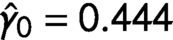 $\hat {\gamma }_0 = 0.444$
(SE =
 $0.109$
) in the original paper. However, as studied in Section 3, when the no omitted network assumption is violated—for example, people might share information through their kinship network, the estimator is biased for the ANSE specific to the financial network.
Sensitivity analysis
We use the proposed sensitivity analysis methods to investigate the robustness of the original findings to unobserved networks. First, for the parametric sensitivity analysis, we consider three values for each of the two sensitivity parameters, the spillover effect in the unobserved network
 $\lambda \in (0.1, 0.2, 0.4)$
and the overlap
 $\pi _{GU} \in (0.2, 0.4, 0.6)$
, producing a total of nine scenarios. The three values of
 $\lambda $
are chosen to represent different scenarios in which we expect spillover effects in the kinship network is much smaller than, smaller than, or similar to the total spillover effect in the financial network (
 $\hat {\gamma }_0 = 0.444$
). Similarly, the three values of
 $\pi _{GU}$
cover from small to large overlaps. For the nonparametric sensitivity analysis, we also investigate three values for each of the two sensitivity parameters
 $\mathrm {MR}_{UY} \in (1.3, 1.5, 1.8)$
and the overlap
 $\mathrm {RR}_{GU} \in (1.3, 1.5, 1.8)$
. Although these are relatively small risk and mean ratios (e.g., see table 1 in Ding and VanderWeele (Reference Ding and VanderWeele2016)), we see below that substantive conclusions change according to different sensitivity parameters. Finally, while the original paper uses a linear regression without weights, we use a weighted linear regression with weights
 $w_i^{\mathtt {B}} = 1/\Pr (T_i, G_i)$
as proposed in Section 4 for both analyses.
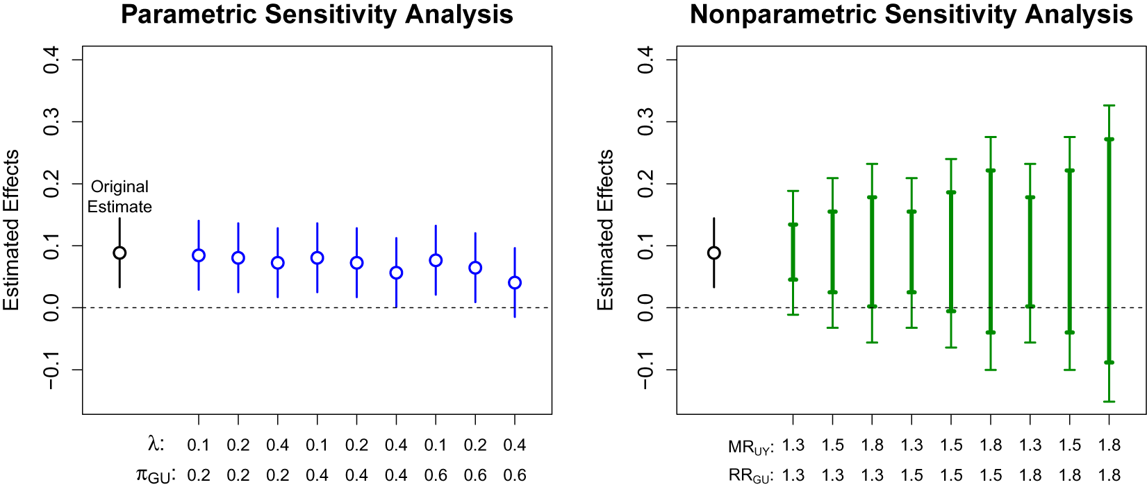
Figure 3 presents results from the parametric (left) and nonparametric sensitivity analysis (right). In the left panel, the leftmost point shows an estimate of the ANSE that ignores the unobserved kinship network with its 95% CI (
 $8.87$
percentage point; 95% CI =
 $[3.31, 14.42]$
). The nine other points represent estimates from the parametric sensitivity analysis with their 95% CI. Importantly, point estimates are relatively stable over a range of sensitivity parameters and the 95% CI covers zero only when the effect in the unobserved kinship network is large (
 $\lambda = 0.4$
) and the overlap between the observed financial network and the unobserved kinship network is relatively large (
 $\pi _{GU} = 0.6$
). Thus, the parametric sensitivity analysis suggests that, while point estimates of the ANSE specific to the observed financial network are smaller than the original estimates, estimates are still positive and statistically significant at the conventional level of
 $0.05$
. Although this parametric sensitivity analysis is simple and intuitive, it requires the parametric linear additive assumption as discussed in Section 4.1. We now turn to the nonparametric sensitivity analysis which requires weaker assumptions at the expense of efficiency.
Parametric and nonparametric sensitivity analysis for the field network experiment in China. Note: The left (right) panel reports the parametric (nonparametric) sensitivity analysis with different sensitivity parameters. In both panels, the leftmost point shows an estimate of the ANSE that ignores unobserved networks. In the left panel, the nine other points represent estimates from the parametric sensitivity analysis with their 95% confidence intervals. In the right panel, the thick bars represent nonparametric bounds on the ANSE and the thin bars are their 95% confidence intervals.

The right panel of Figure 3 shows results of the nonparametric sensitivity analysis where the leftmost point reproduces the same ANSE estimate that ignores the unobserved kinship network as a reference point. The thick bars represent nonparametric bounds on the ANSE and the thin bars are their 95% CI. Although lower bounds are positive for small bias scenarios, such as
 $(MR_{UY}, RR_{GU}) = (1.3, 1.3), (1.5, 1.3), (1.3, 1.5),$
all the 95% CI are inconclusive about the sign of the ANSE. Importantly, this result reveals that the positive ANSE estimates are sensitive to different assumptions about unobserved networks in the nonparametric sensitivity analysis, in contrast to the parametric sensitivity analysis above.
This difference in results from the parametric and nonparametric sensitivity analysis can arise for two reasons. First, the linear additive assumption (Assumption 3) required for the parametric sensitivity analysis could be violated and therefore, the nonparametric bounds are more credible. Second, the nonparametric bounds are in general less efficient than parametric methods and thus, large nonparametric bounds simply indicate insufficient statistical power for detecting the ANSE nonparametrically. In this China experiment, as the original authors detect the nonlinearity in the total spillover effect in the financial network (table 3 of Cai et al.(Reference Cai, De Janvry and Sadoulet2015)), it is more likely that the linear additive assumption is violated and thus, the nonparametric sensitivity analysis is more credible. In practice, it is important to conduct both parametric and nonparametric sensitivity analysis methods as they are complementary and evaluate the robustness of the ANSE estimates under different assumptions.
7 Concluding Remarks
Although early work in the causal inference literature has assumed no interference, a growing number of both applied and methodological papers now explicitly incorporate spillover effects to understand causal interdependence across people. In this paper, we propose a framework for analyzing spillover effects in common social science settings of multiple networks, and introduce a new causal estimand, the average network-specific spillover effect (ANSE), to separately quantify the amount of spillover effects in each network. We show that the unbiased estimation of the ANSE requires an often-violated assumption of no omitted network. Unlike conventional omitted variable bias, the bias due to unobserved networks remains even when treatment assignment is randomized and when the network of interest and unobserved networks are independently generated. To account for this bias, we provide parametric and nonparametric sensitivity analysis methods, with which researchers can assess the robustness of causal conclusions to unobserved networks. The proposed methods are illustrated by two common types of network experiments; an online social network experiment and a network field experiment.
There are a number of future extensions that can further improve the methodologies proposed in this paper. First, although we made the assumption of stratified interference throughout this paper, we can potentially derive the exact bias formula and sensitivity analysis methods without it. This direction will be particularly important since not only the no omitted network assumption, but also the assumption of stratified interference might be strong in many applied settings. Second, while we focused on the estimation of the ANSE in this paper, it would also be of significant interest to study how to incorporate observed and unobserved networks into the rich literature of the Fisher randomization test for interference (e.g., Rosenbaum Reference Rosenbaum2007; Aronow Reference Aronow2012; Bowers et al. Reference Bowers, Fredrickson and Panagopoulos2013; Athey et al. Reference Athey, Eckles and Imbens2018; Basse et al. Reference Basse, Feller and Toulis2019). Third, it is useful to study how we can effectively incorporate a supplementary survey to estimate the overlap between the main network of interest and an unobserved network. For example, in an online network experiment, even though it might be difficult to measure an offline face-to-face network for every subject in the experiment, researchers can use a network survey method (e.g., Bisbee and Larson Reference Bisbee and Larson2017) to randomly sample subjects and use the estimated overlap for the sensitivity analysis. Fourth, this paper primarily focused on the bias due to unobserved networks, but another important extension would be to study implications of omitted relevant networks to variance estimation. A promising approach would be to consider a range of sensitivity parameters and compute the worst-case confidence interval (e.g., Berger and Boos Reference Berger and Boos1994; Aronow et al. Reference Aronow, Crawford and Zubizarreta2016). Finally, as discussed in the paper, the estimation accuracy is often of concern in settings with multiple networks. Thus, it would be useful to extend the literature on experimental design for spillover effects to settings of multiple networks and study how to design the optimal experiment (e.g., Hudgens and Halloran Reference Hudgens and Halloran2008; Sinclair et al. Reference Sinclair, McConnell and Green2012; Basse and Airoldi Reference Basse and Airoldi2018; Bowers et al. Reference Bowers, Desmarais, Frederickson, Ichino, Lee and Wang2018; Jagadeesan et al. Reference Jagadeesan, Pillai and Volfovsky2020).
Supplementary Appendix
Appendix A Details of Setup
We describe regularity conditions for the support of treatment exposure probabilities to ensure well-defined causal estimands.
The required regularity conditions are as follows: (1) the support of
 $\Pr (G_i=g, U_i=u | T_i=1)$
is equal to the support of
 $\Pr (G_i=g, U_i=u | T_i=0)$
for all i, and (2) the support of
 $\Pr (U_i=u | T_i=d, G_i=g^H)$
is equal to the support of
 $\Pr (U_i=u | T_i=d, G_i=g^L)$
for all i. We discuss them in order.
When we define the unit level direct effect, we avoid ill-defined causal effects by focusing on settings where the support of
 $\Pr (G_i=g, U_i=u \mid T_i=1)$
is equal to the support of
 $\Pr (G_i=g, U_i=u \mid T_i=0)$
for all i. This can be violated when the total number of treated units is small so that for some
 $(g, u)$
,
 $\Pr (G=g, U=u | T_i=1) =0$
and
 $\Pr (G=g, U=u | T_i=0)>0.$
One extreme example is that when we use complete randomization with the total number of treated units equal to
 $1$
. In this case, whenever
 $T_i=1$
,
 $\Pr (G=g, U=u | T_i=1) =0$
for all
 $(g,u)$
, but when
 $T_i=0$
,
 $\Pr (G=g, U=u | T_i=0)>0$
for some
 $(g,u).$
Another extreme example is that the total number of treated units is too large. For example, when we use complete randomization with the total number of treated units equal to
 $N-1$
. In this case, whenever
 $T_i=0$
,
 $\Pr (G=g, U=u | T_i=0) =0$
for all
 $(g,u)$
except for
 $(g, u) = (1,1)$
, but when
 $T_i=1$
,
 $\Pr (G=g, U=u | T_i=1)>0$
for some
 $(g,u)$
other than
 $(g, u) = (1,1)$
. It is clear that when researchers use a Bernoulli design, the support of
 $\Pr (G_i=g, U_i=u \mid T_i=1)$
is equal to the support of
 $\Pr (G_i=g, U_i=u \mid T_i=0)$
for all i.
When we define the unit level network-specific spillover effect, we avoid ill-defined causal effects by focusing on settings where
 $\Pr (U_i=u \mid T_i=d, G_i=g^H)$
and
 $\Pr (U_i=u \mid T_i=d, G_i=g^L)$
have the same support for all i. This requires that
 $g^H$
and
 $g^L$
are small enough so that the distribution over the fraction of treated neighbors in network
 $\mathcal {U}$
is not restricted, especially
 $\Pr (U_i=0 \mid T_i=d, G_i=g^H)> 0$
and
 $\Pr (U_i=0 \mid T_i=d, G_i=g^L)> 0$
for all i. Formally,
 $g^H, g^L \leq g_s$
where
 $g_s \equiv \underset {i}{\min } \{1- |\mathcal {N}^{(\mathcal {G},\mathcal {U})}_i|/|\mathcal {N}^{\mathcal {G}}_i|\}$
.
The desired support condition can be violated when the total number of treated units is too small so that for some u,
 $\Pr (U=u | T_i=1, G_i=g^H) =0$
and
 $\Pr (U=u | T_i=1, G_i=g^L)>0$
. One extreme example is that when we use complete randomization with the total number of treated units equal to
 $1 + g^H \times |\mathcal {N}^{\mathcal {G}}_i|.$
In this case, whenever
 $G_i=g^H$
,
 $\Pr (U=u | T_i=1, G_i=g^H) =0$
for all
 $u> |\mathcal {N}^{(\mathcal {G},\mathcal {U})}_i|/|\mathcal {N}^{\mathcal {U}}_i|$
, but when
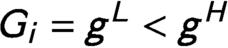 $G_i=g^L < g^H$
,
 $\Pr (U=u | T_i=0, G_i=g^L)>0$
for some
 $u> |\mathcal {N}^{(\mathcal {G},\mathcal {U})}_i|/|\mathcal {N}^{\mathcal {U}}_i|$
. Finally, it is clear that
 $\Pr (U_i=u \mid T_i=d, G_i=g^H)$
and
 $\Pr (U_i=u \mid T_i=d, G_i=g^L)$
have the same support for all i if researchers use a Bernoulli design and
 $g^H, g^L \leq g_s$
.
Appendix B Connection between Total Spillover Effects and Network-Specific Spillover Effects
Here, we connect the ANSE to the popular estimand in the literature. In particular, we show that the ANSE can be seen as the decomposition of the average total spillover effect (Hudgens and Halloran Reference Hudgens and Halloran2008).
First, by extending Hudgens and Halloran (Reference Hudgens and Halloran2008) to settings with multiple networks, the individual average potential outcome are defined as follows.
 $$ \begin{align} \overline{Y}_i (d,g) \equiv \sum_{u \in \Delta_i^u} Y_i(d, g, u) \Pr(U_i=u \mid T_i=d, G_i=g), \end{align} $$
where the potential outcome of individual i is averaged over the conditional distribution of the treatment assignment
 $\Pr (U_i=u \mid T_i=d, G_i=g).$
Here, the individual average potential outcome represents the expected outcome of unit i when she receives the direct treatment d and the treated proportion g in network
 $\mathcal {G}$
. Taking the difference in the two individual average potential outcomes, the average total spillover effect (ATSE) in network
 $\mathcal {G}$
is defined as follows (Halloran and Hudgens Reference Halloran and Hudgens2016).Footnote
8
 $$ \begin{align} \psi(g^H, g^L;d) \ \equiv \ \frac{1}{N} \sum_{i=1}^N \{\overline{Y}_i (d, g^H) - \overline{Y}_i (d, g^L)\}. \end{align} $$
This causal quantity is the total spillover effect of changing the treated proportion in network
 $\mathcal {G}$
from
 $g^L$
to
 $g^H$
as the following decomposition of the ATSE demonstrates.
 $$ \begin{align} &\psi(g^H, g^L;d) = \tau(g^H, g^L;d) + \\[5pt] &\frac{1}{N} \!\sum_{i=1}^N \!\left\{\!\sum_{u \in \Delta^u_i}\! \{Y_i(d, g^H, u) -Y_i(d, g^H,u^\prime)\} \{\Pr (U_i=u \mid T_i=d, G_i=g^H) - \Pr(U_i=u \mid T_i=d, G_i=g^L)\}\! \right\}, \nonumber \end{align} $$
for any
 $u^\prime \in \Delta _i^u$
. The first term is the ANSE in network
 $\mathcal {G}$
(Definition 3), which quantifies the spillover effect specific to network
 $\mathcal {G}$
. The second term represents the spillover effect in
 $\mathcal {U}$
,
 $Y_i(d, g^H, u) -Y_i(d, g^H,u^\prime )$
, weighted by the change in the conditional distribution of
 $U_i$
due to the change in
 $G_i$
,
 $\Pr (U_i=u \mid T_i=d, G_i=g^H) - \Pr (U_i=u \mid T_i=d, G_i=g^L).$
This is because
 $U_i$
, the treated proportion of neighbors in the other network
 $\mathcal {U}$
, is not fixed at constant and thus, they change as
 $G_i$
, the treated proportion of neighbors in
 $\mathcal {G}$
, changes. Thus, the ATSE captures the sum of the spillover effect specific to network
 $\mathcal {G}$
and the spillover effect specific to
 $\mathcal {U}$
induced by the change in
 $U_i$
associated with the change in
 $G_i$
. For example, the ATSE of changing from
 $g^L$
to
 $g^H$
on the Facebook network captures two spillover effects together; (1) the spillover effect specific to the Facebook and (2) the spillover effect in the face-to-face network. This is because the treated proportion in the offline network
 $U_i$
is associated with the change in the treated proportion in the Facebook network
 $G_i$
. We discuss this issue in further details when we derive the exact bias formula in Section 3. When network
 $\mathcal {U}$
, such as the offline network, is causally irrelevant, the ATSE is equal to the ANSE in the Facebook network, but in general, the two estimands do not coincide.
While both the ATSE and the ANSE quantify spillover effects, their substantive meanings differ. The ATSE is useful when researchers wish to know the total amount of spillover effects that result from interventions on an observed network. For instance, politicians decided to run online campaigns on Twitter and want to estimate the total amount of spillover effects they can induce by their Twitter messages. These politicians might not be interested in distinguishing whether the spillover effects arise through Twitter or through unobserved face-to-face interactions. Thus, the ATSE is of relevance when the target network is predetermined and the mechanism can be ignored.
In contrast, the ANSE is essential for disentangling different channels through which spillover effects arise. It is the main quantity of interest when researchers wish to examine the causal role of individual networks or to discover the most causally relevant network to target. For example, it is of scientific interest to distinguish how much spillover effects arise through the Twitter network or through offline communications. By estimating the ANSE, researchers can learn about the importance of online human interactions.
Appendix C Proofs
This section provides proofs for all theorems in the paper.
C.1 Proof of Theorem 1
C.1.1 Average Direct Effect
First, we rewrite the estimator with the standard IPW representation.
 $$ \begin{align*} & \hat{\delta} \\ & = \frac{1}{N} \sum_{i=1}^N \mathbf{1}\{T_i=1\} \tilde{w}_i Y_i - \frac{1}{N} \sum_{i=1}^N \mathbf{1}\{T_i=0\} \tilde{w}_i Y_i \\ & = \frac{1}{N} \sum_{i=1}^N \sum_{(g,u) \in \Delta^{gu}_i} \Pr (G_i=g, U_i=u) \biggl\{ \frac{\mathbf{1}\{T_i=1, G_i=g, U_i=u\} Y_i}{\Pr(T_i=1, G_i=g, U_i=u)} - \frac{\mathbf{1}\{T_i=0, G_i=g, U_i=u\} Y_i}{\Pr(T_i=0, G_i=g, U_i=u)}\biggr\}. \end{align*} $$
Then, the theorem follows from the standard proof for the IPW estimator.
 $$ \begin{align*} & \mathbb{E}[\hat{\delta}] \\ & = \frac{1}{N} \sum_{i=1}^N \sum_{(g,u) \in \Delta^{gu}_i} \Pr (G_i=g, U_i=u)\ \times \\ & \hspace{1in} \biggl\{ \frac{\mathbb{E}[\mathbf{1}\{T_i=1, G_i=g, U_i=u\} Y_i]}{\Pr(T_i=1, G_i=g, U_i=u)} - \frac{\mathbb{E}[\mathbf{1}\{T_i=0, G_i=g, U_i=u\} Y_i]}{\Pr(T_i=0, G_i=g, U_i=u)} \biggr\} \\ & = \frac{1}{N} \sum_{i=1}^N \sum_{(g,u) \in \Delta^{gu}_i} \Pr (G_i=g, U_i=u)\ \times \\ & \hspace{1in} \biggl\{ \frac{\Pr(T_i=1, G_i=g, U_i=u) Y_i(1, g, u)}{\Pr(T_i=1, G_i=g, U_i=u)} - \frac{\Pr(T_i=0, G_i=g, U_i=u) Y_i(0,g,u)}{\Pr(T_i=0, G_i=g, U_i=u)} \biggr\} \\ & = \frac{1}{N} \sum_{i=1}^N \sum_{(g,u) \in \Delta^{gu}_i} \Pr (G_i=g, U_i=u) \{ Y_i(1, g, u) - Y_i(0,g,u) \} \\ & = \delta \end{align*} $$
where the second equality follows from the consistency of potential outcomes. □
C.1.2 Average Network-Specific Effect
First, we rewrite the estimator with the standard IPW representation.
 $$ \begin{align*} & \hat{\tau} \\ & = \frac{1}{N} \sum_{i=1}^N \mathbf{1}\{T_i = d, G_i = g^H\} w_i Y_i - \frac{1}{N} \sum_{i=1}^N \mathbf{1}\{T_i = d, G_i = g^L\} w_i Y_i \\ & = \frac{1}{N} \sum_{i=1}^N \sum_{u \in \Delta_i^u} \Pr (U_i=u \mid T_i=d, G_i = g^L)\ \times \\ & \hspace{1.5in} \biggl\{ \frac{\mathbf{1}\{T_i=d, G_i=g^H, U_i=u\} Y_i}{\Pr(T_i=d, G_i=g^H, U_i=u)} - \frac{\mathbf{1}\{T_i=d, G_i=g^L, U_i=u\} Y_i}{\Pr(T_i=d, G_i= g^L, U_i=u)} \biggr\}, \end{align*} $$
Then, the theorem follows from the standard proof for the IPW estimator.
 $$ \begin{align*} & \mathbb{E}[\hat{\tau}(g,g^\prime; d)] \\ & = \frac{1}{N} \sum_{i=1}^N \sum_{u \in \Delta_i^u} \Pr (U_i=u \mid T_i=d, G_i = g^L)\ \times \\ & \hspace{1in} \biggl\{ \frac{\mathbb{E}[\mathbf{1}\{T_i=d, G_i=g^H, U_i=u\} Y_i]}{\Pr(T_i=d, G_i=g^H, U_i=u)} - \frac{\mathbb{E}[\mathbf{1}\{T_i=d, G_i=g^L, U_i=u\} Y_i]}{\Pr(T_i=d, G_i=g^L, U_i=u)} \biggr\} \\ & = \frac{1}{N} \sum_{i=1}^N \sum_{u \in \Delta_i^u} \Pr (U_i=u \mid T_i=d, G_i = g^L)\ \times \\ & \hspace{0.5in} \biggl\{ \frac{\Pr (T_i=d, G_i=g^H, U_i=u) Y_i(d,g^H,u)}{\Pr(T_i=d, G_i=g^H, U_i=u)} - \frac{\Pr (T_i=d, G_i=g^L, U_i=u) Y_i(d, g^L,u)}{\Pr (T_i=d, G_i=g^L, U_i=u)} \biggr\} \\ & = \frac{1}{N} \sum_{i=1}^N \sum_{u \in \Delta_i^u} \Pr (U_i=u \mid T_i=d, G_i = g^L) \{Y_i(d,g^H,u) - Y_i(d,g^L,u)\} \\ & = \tau (g^H,g^L; d), \end{align*} $$
which completes the proof. □
C.2 Proof of Theorem 2
The expectation of an estimator
 $\hat {\tau }_B(g^H, g^L; d)$
is
 $$ \begin{align*} & \mathbb{E}[\hat{\tau}_B(g^H, g^L; d)] = \frac{1}{N} \sum_{i=1}^N \biggl\{ \mathbb{E}[Y_i \mid T_i = d, G_i = g^H] - \mathbb{E}[Y_i \mid T_i = d, G_i = g^L] \biggr\} \\ & = \frac{1}{N} \sum_{i=1}^N \sum_{u \in \Delta^u_i} \biggl\{ Y_i (d,g^H,u) \Pr(U_i=u \mid T_i=d, G_i=g^H) - Y_i(d, g^L,u) \Pr(U_i=u \mid T_i=d, G_i=g^L) \biggr\}. \end{align*} $$
Therefore, we get
 $$ \begin{align*} & \mathbb{E}[\hat{\tau}_B(g^H, g^L; d)] - \tau(g^H, g^L; d) \\ & = \frac{1}{N} \sum_{i=1}^N \sum_{u \in \Delta^u_i} \left\{ Y_i (d,g^H,u) \{\Pr(U_i=u \mid T_i=d, G_i=g^H) - \Pr(U_i=u \mid T_i=d, G_i = g^L)\}\right. \\ & \qquad - Y_i(d, g^L,u) \left.\{\Pr(U_i=u \mid T_i=d, G_i=g^L) - \Pr(U_i=u \mid T_i=d, G_i = g^L)\} \right\} \\ & = \frac{1}{N} \sum_{i=1}^N \sum_{u \in \Delta^u_i} \left\{ \{Y_i (d, g^H,u) - Y_i(d, g^H, u^\prime)\}\right. \\ & \hspace{1.2in} \left.\times\ \{\Pr(U_i=u \mid T_i=d, G_i=g^H) - \Pr(U_i=u \mid T_i=d, G_i = g^L)\} \right\}. \end{align*} $$
for any
 $u^\prime \in \Delta ^u$
. □
C.2.1 Lemma: Bias in ADE
First, we can rewrite the estimator as the standard IPW estimator.
 $$ \begin{align*} \hat{\delta}_B & = \frac{1}{N} \sum_{i=1}^N \mathbf{1}\{T_i=1\} \tilde{w}^{\mathtt{B}}_i Y_i - \frac{1}{N} \sum_{i=1}^N \mathbf{1}\{T_i=0\} \tilde{w}^{\mathtt{B}}_i Y_i \\ & = \frac{1}{N} \sum_{i=1}^N \sum_{g \in \Delta^{g}_i} \Pr (G_i=g) \biggl\{ \frac{\mathbf{1}\{T_i=1, G_i=g\} Y_i}{\Pr(T_i=1, G_i=g)} - \frac{\mathbf{1}\{T_i=0, G_i=g\} Y_i}{\Pr(T_i=0, G_i=g)} \biggr\}. \end{align*} $$
We have the following equality for any g,
 $$ \begin{align*} & \mathbb{E}[\mathbf{1}\{T_i=d, G_i=g\} Y_i] \\ &= \mathbb{E}[ \sum_{u \in \Delta^u_i(g)} \mathbf{1}\{T_i=d, G_i=g, U_i=u\} Y_i(d,g,u)] \\ &= \sum_{u \in \Delta^u_i(g)} \Pr(T_i=d, G_i=g, U_i=u) Y_i(d,g,u) \end{align*} $$
where
 $\Delta _i^u(g)$
is the support
 $\{u: \Pr (U_i=u \mid G_i=g)>0\}.$
Therefore, the expectation of
 $\hat {\delta }_B$
is
 $$ \begin{align*} & \mathbb{E}[\hat{\delta}_B] \\ & = \frac{1}{N} \sum_{i=1}^N \sum_{g \in \Delta^{g}_i} \Pr (G_i=g) \bigg\{ \frac{\mathbb{E}[\mathbf{1}\{T_i=1, G_i=g\} Y_i]}{\Pr(T_i=1, G_i=g)} - \frac{\mathbb{E}[\mathbf{1}\{T_i=0, G_i=g\} Y_i]}{\Pr(T_i=0, G_i=g)} \bigg\} \\ &= \frac{1}{N} \sum_{i=1}^N \sum_{g \in \Delta^{g}_i} \Pr (G_i=g) \\ & \quad \Bigg\{\sum_{u \in \Delta_i^u(g)} \bigg\{ \frac{\Pr(T_i=1, G_i=g, U_i=u) Y_i(1,g,u)}{\Pr(T_i=1, G_i=g)} - \frac{\Pr(T_i=0, G_i=g, U_i=u) Y_i(0,g,u)}{\Pr(T_i=0, G_i=g)} \bigg\} \Bigg\}\\ &= \frac{1}{N} \sum_{i=1}^N \sum_{g \in \Delta^{g}_i} \Pr (G_i=g) \\ & \quad \Bigg\{ \sum_{u \in \Delta_i^u(g)} \bigg\{ Y_i(1,g,u) \Pr(U_i=u \mid T_i=1, G_i=g) - Y_i(0,g,u) \Pr(U_i=u \mid T_i=0, G_i=g) \bigg\} \Bigg\}. \end{align*} $$
Then, we have
 $$ \begin{align*} & \mathbb{E}[\hat{\delta}_B] - \delta \\ &= \frac{1}{N} \sum_{i=1}^N \sum_{g \in \Delta^{g}_i} \mathrm{Pr}_i (G_i=g) \left\{ \sum_{u \in \Delta_i^u} Y_i (1, g, u) \{ \mathrm{Pr}_i(U_i=u \mid T_i=1, G_i=g) - \mathrm{Pr}_i(U_i=u \mid G_i=g)\}\right. \\ & \quad - \sum_{u \in \Delta_i^u} Y_i (0, g^\prime, u) \left.\{ \Pr(U_i=u \mid T_i=0, G_i=g) - \Pr(U_i=u \mid G_i=g) \}\vphantom{\sum_{u \in \Delta_i^u}}\right\}\\ &= \frac{1}{N} \sum_{i=1}^N \sum_{g \in \Delta^{g}_i} \Pr (G_i=g) \\ & \quad \left\{ \sum_{u \in \Delta_i^u(g)} \{Y_i (1, g, u) - Y_i(1, g, u^\prime)\} \{ \Pr(U_i=u \mid T_i=1, G_i=g) - \Pr(U_i=u \mid G_i=g)\}\right. \\ &\quad - \sum_{u \in \Delta_i^u(g)} \{Y_i (0, g^\prime, u) - Y_i(0, g^\prime, u^\prime)\} \left.\{ \Pr(U_i=u \mid T_i=0, G_i=g) - \Pr(U_i=u \mid G_i=g) \}\vphantom{\sum_{u \in \Delta_i^u(g)}}\right\}, \end{align*} $$
which completes the proof. □
C.3 Proof of Theorem 3
Using Theorem 2, under Assumption 3,
 $$ \begin{align*} & \mathbb{E}[\hat{\tau}_B(g^H, g^L; d)] - \tau(g^H, g^L; d) \\ & = \lambda \times \frac{1}{N} \sum_{i=1}^N \{\mathbb{E}[U_i=u \mid T_i=d, G_i=g^H] - \mathbb{E}[U_i=u \mid T_i=d, G_i=g^L]\}. \end{align*} $$
From here, we focus on
 $\mathbb {E}[U_i \mid T_i=d, G_i=g^H]$
. For notational simplicity, we use
 $n_{G}(i)$
to denote the number of neighbors in the network
 $\mathcal {G}$
for individual i and
 $n_U(i)$
is similarly defined. Also, for individual i, let
 $\pi _{GU}(i)$
be the fraction of the neighbors in
 $\mathcal {U}$
who are neighbors in
 $\mathcal {G}$
as well. Formally,
 $n_G(i) = |\mathcal {N}^{\mathcal {G}}_i|, n_U(i) = |\mathcal {N}^{\mathcal {U}}_i|$
and
 $ \pi _{GU}(i) = |\mathcal {N}^{(\mathcal {G},\mathcal {U})}_i| /|\mathcal {N}^{\mathcal {U}}_i|.$
First, we consider Bernoulli randomization with probability p. Under this setting,
 $$ \begin{align*} & \mathbb{E}[U_i \mid T_i=t, G_i=g^H] = \pi_{GU}(i) \times g^H + (1 - \pi_{GU}(i)) \times p. \end{align*} $$
Therefore, we have
 $$ \begin{align*} & \mathbb{E}[\hat{\tau}_B(g^H, g^L; d)] - \tau(g^H, g^L; d) \\ & = \lambda \times \frac{1}{N} \sum_{i=1}^N \{\mathbb{E}[U_i=u \mid T_i=d, G_i=g^H] - \mathbb{E}[U_i=u \mid T_i=d, G_i=g^L]\}. \\ & = \lambda \times \frac{1}{N} \sum_{i=1}^N \pi_{GU}(i) \times (g^H - g^L)\\ & = \lambda \times \pi_{GU} \times (g^H - g^L). \end{align*} $$
where the final equality follows from the definition of
 $\pi _{GU}$
.
Next, we consider complete randomization with the number of treated units K. Under this setting,
 $$ \begin{align*} & \mathbb{E}[U_i \mid T_i=d, G_i=g^H] \\ & = \frac{n_{U}(i) \times \pi_{GU}(i) \times g^H }{n_U(i)} + (1 - \pi_{GU}(i)) \frac{K- d - n_G(i) \times g^H}{N - 1 - n_{G}(i)}\\ & = \pi_{GU}(i) \times g^H + (1 - \pi_{GU}(i)) \frac{K- d - n_G(i) \times g^H}{N - 1- n_{G}(i)}\\ & = \bigl\{ \pi_{GU}(i) - \frac{n_G(i)}{N-1-n_G(i)} (1-\pi_{GU}(i)) \bigr\} g^H + \frac{K-d}{N-1-n_{G}(i)}(1 - \pi_{GU}(i)) \end{align*} $$
When N is much larger than
 $n_G(i)$
,
 $ n_G(i) /(N - 1 - n_{G}(i)) \approx 0$
. Then, we have
 $$ \begin{align*} & \mathbb{E}[U_i \mid T_i=d, G_i=g^H] \approx \pi_{GU}(i) g^H + \frac{K-d}{N-1-n_{G}(i)}(1 - \pi_{GU}(i)), \\ & \mathbb{E}[U_i \mid T_i=d, G_i=g^H] - \mathbb{E}[U_i=u \mid T_i=d, G_i=g^L] \approx \pi_{GU}(i) (g^H - g^L). \end{align*} $$
Therefore, when N is much larger than
 $n_G(i)$
for all i, we get the simplified bias formula.
 $$ \begin{align*} & \mathbb{E}[\hat{\tau}_B(g^H, g^L; d)] - \tau(g^H, g^L; d) \\ & = \lambda \times \frac{1}{N} \sum_{i=1}^N \{\mathbb{E}[U_i=u \mid T_i=d, G_i=g^H] - \mathbb{E}[U_i=u \mid T_i=d, G_i=g^L]\}. \\ & \approx \lambda \times \frac{1}{N} \sum_{i=1}^N \pi_{GU}(i) \times (g^H - g^L)\\ & = \lambda \times \pi_{GU} \times (g^H - g^L). \end{align*} $$
Finally, we consider a situation when N is not large enough to have the aforementioned approximation. Suppose
 $N \approx (C+1) n_G(i) + 1$
for all i. Then,
 $$ \begin{align*} & \mathbb{E}[U_i \mid T_i=d, G_i=g^H] \approx \bigl\{ \frac{C+1}{C} \pi_{GU}(i) - \frac{1}{C} \bigr\} \times g^H + \frac{K-d}{N-1-n_{G}(i)}(1 - \pi_{GU}(i)), \\ & \mathbb{E}[U_i \mid T_i=d, G_i=g^H] - \mathbb{E}[U_i=u \mid T_i=d, G_i=g^L] \approx \bigl\{ \frac{C+1}{C} \pi_{GU}(i) - \frac{1}{C} \bigr\} (g^H - g^L). \end{align*} $$
Therefore, the bias can be written as,
 $$ \begin{align} & \mathbb{E}[\hat{\tau}_B(g^H, g^L; d)] - \tau(g^H, g^L; d) \notag \\ & = \lambda \times \frac{1}{N} \sum_{i=1}^N \{\mathbb{E}[U_i=u \mid T_i=d, G_i=g^H] - \mathbb{E}[U_i=u \mid T_i=d, G_i=g^L]\}. \notag \\ & \approx \lambda \times \bigl\{ \frac{C+1}{C} \times \frac{1}{N} \sum_{i=1}^N \pi_{GU}(i) - \frac{1}{C} \bigr\} \times (g^H - g^L). \notag \\ & = \lambda \times \bigl\{ \frac{C+1}{C} \pi_{GU} - \frac{1}{C} \bigr\}\times (g^H - g^L). \end{align} $$
□
C.4 Proof of Theorem 4
First, we set the following notations. We define the support
 $\Delta ^u_s$
to be the support
 $\Delta _i^u$
for all i with
 $S_i=s$
. We drop subscript s whenever it is obvious from contexts. For
 $\bar {g} \in \{g^H, g^L\}$
,
 $$ \begin{align*} r_{\bar{g}} (u) & \equiv \frac{1}{N} \sum_{i: S_i=s} Y_i(d, \bar{g}, u) \\ v_{g^H} (\bar{g}) & \equiv \frac{\sum_{u \in \Delta_s^u} \{ r_{\bar{g}} (u) - \min\nolimits_u r_{\bar{g}} (u) \} \ \Pr(U_i=u \mid T_i=d, G_i=g^H)}{\max\nolimits_u r_{\bar{g}} (u) - \min\nolimits_u r_{\bar{g}} (u) } \\ v_{g^L} (\bar{g}) & \equiv \frac{\sum_{u \in \Delta_s^u} \{ r_{\bar{g}} (u) - \min\nolimits_u r_{\bar{g}} (u) \} \Pr(U_i=u \mid T_i=d, G_i=g^L)}{\max\nolimits_u r_{\bar{g}} (u) - \min\nolimits_u r_{\bar{g}} (u) } \\ \Gamma (\bar{g}) & \equiv \frac{v_{g^H} (\bar{g}) }{v_{g^L}(\bar{g})} = \frac{\sum_{u \in \Delta_s^u} \{ r_{\bar{g}} (u) - \min\nolimits_u r_{\bar{g}} (u) \} \Pr(U_i=u \mid T_i=d, G_i=g^H)}{\sum_{u \in \Delta_s^u} \{ r_{\bar{g}} (u) - \min\nolimits_u r_{\bar{g}} (u) \} \Pr(U_i=u \mid T_i=d, G_i=g^L)} \\ MR^{obs}(g^H, g^L ; s) & \equiv \frac{\sum_{u \in \Delta_s^u} r_{g^H} (u) \Pr(U_i=u \mid T_i=d, G_i=g^H)}{\sum_{u \in \Delta_s^u} r_{g^L} (u) \Pr(U_i=u \mid T_i=d, G_i=g^L)}\\ MR^{true}_{\bar{g}}(g^H, g^L; s) & \equiv \frac{\sum_{u \in \Delta_s^u} r_{g^H} (u) \Pr(U_i=u \mid T_i=d, G_i=\bar{g})} {\sum_{u \in \Delta_s^u} r_{g^L} (u) \Pr(U_i=u \mid T_i=d, G_i=\bar{g})} \end{align*} $$
where
 $0 \leq v_{g^H} (\bar {g}), v_{g^L} (\bar {g})\leq 1$
because of non-negative outcomes.
Lemma 1 For
 $(g^H, g^L)$
,
 $$ \begin{align*} \frac{MR^{obs}(g^H, g^L;s)}{MR^{true}_{g^L}(g^H, g^L; s)} \ \leq \ B \ \ \ & \ \ \ \frac{MR^{obs} (g^H, g^L; s)}{MR^{true}_{g^H}(g^H, g^L; s)} \ \leq \ B,\\ \frac{MR^{obs}(g^L, g^H;s)}{MR^{true}_{g^L}(g^L, g^H; s)} \ \leq \ B \ \ \ & \ \ \ \frac{MR^{obs} (g^L, g^H; s)}{MR^{true}_{g^H}(g^L, g^H; s)} \ \leq \ B. \end{align*} $$
Proof
This proof closely follows Ding and VanderWeele (Reference Ding and VanderWeele2016). The key difference is that we study bias due to an unmeasured relevant network in the presence of interference in multiple networks in contrary to bias due to an unmeasured confounder in observational studies without interference (Ding and VanderWeele Reference Ding and VanderWeele2016).
For
 $\bar {g} \in \{g^H, g^L\}$
and s,
 $$ \begin{align*} \Gamma (\bar{g}) & = \frac{\sum_{u \in \Delta_s^u} \{ r_{\bar{g}} (u) - \min\nolimits_u r_{\bar{g}} (u) \} \Pr(U_i=u \mid T_i=d, G_i=g^H)}{\sum_{u \in \Delta_s^u} \{ r_{\bar{g}} (u) - \min\nolimits_u r_{\bar{g}} (u) \} \Pr(U_i=u \mid T_i=d, G_i=g^L)} \\ & = \frac{\sum_{u \in \Delta_s^u} \{ r_{\bar{g}} (u) - \min\nolimits_u r_{\bar{g}} (u) \} \frac{ \Pr(U_i=u \mid T_i=d, G_i=g^H)}{ \Pr(U_i=u \mid T_i=d, G_i=g^L)} \Pr(U_i=u \mid T_i=d, G_i=g^L)} {\sum_{u \in \Delta_s^u} \{ r_{\bar{g}} (u) - \min\nolimits_u r_{\bar{g}} (u) \} \ \Pr(U_i=u \mid T_i=d, G_i=g^L)} \\ & \leq \mathrm{RR}_{GU} \end{align*} $$
Also, for
 $\bar {g} \in \{g^H, g^L\}$
and s,
 $$ \begin{align*} \frac{1}{\Gamma (\bar{g})} & = \frac{\sum_{u \in \Delta_s^u} \{ r_{\bar{g}} (u) - \min\nolimits_u r_{\bar{g}} (u) \} \Pr(U_i=u \mid T_i=d, G_i=g^L)}{\sum_{u \in \Delta_s^u} \{ r_{\bar{g}} (u) - \min\nolimits_u r_{\bar{g}} (u) \} \Pr(U_i=u \mid T_i=d, G_i=g^H)} \\ & = \frac{\sum_{u \in \Delta_s^u} \{ r_{\bar{g}} (u) - \min\nolimits_u r_{\bar{g}} (u) \} \frac{ \Pr(U_i=u \mid T_i=d, G_i=g^L)}{ \Pr(U_i=u \mid T_i=d, G_i=g^H)} \Pr(U_i=u \mid T_i=d, G_i=g^H)} {\sum_{u \in \Delta_s^u} \{ r_{\bar{g}} (u) - \min\nolimits_u r_{\bar{g}} (u) \} \ \Pr(U_i=u \mid T_i=d, G_i=g^H)} \\ & \leq \mathrm{RR}_{GU}. \end{align*} $$
Then, we have
 $$ \begin{align*} & \frac{MR^{obs}(g^H, g^L; s)}{MR^{true}_{g^L}(g^H, g^L; s)} \\ & = \frac{\sum_{u \in \Delta_s^u} r_{g^H} (u) \Pr(U_i=u \mid T_i=d, G_i=g^H)}{\sum_{u \in \Delta_s^u} r_{g^L} (u) \Pr(U_i=u \mid T_i=d, G_i=g^L)} \times \frac{\sum_{u \in \Delta_s^u} r_{g^L} (u) \Pr(U_i=u \mid T_i=d, G_i=g^L)} {\sum_{u \in \Delta_s^u} r_{g^H} (U) \Pr(U_i=u \mid T_i=d, G_i=g^L)}\\ & = \frac{\sum_{u \in \Delta_s^u} r_{g^H} (u) \Pr(U_i=u \mid T_i=d, G_i=g^H)}{\sum_{u \in \Delta_s^u} r_{g^H} (u) \Pr(U_i=u \mid T_i=d, G_i=g^L)}\\ & = \frac{\{ \max\nolimits_u r_{g^H} (u) - \min\nolimits_u r_{g^H} (u)\} v_{g^H} (g^H) + \min\nolimits_u r_{g^H} (u)}{\{ \max\nolimits_u r_{g^H} (u) - \min\nolimits_u r_{g^H} (u)\} \frac{v_{g^H} (g^H)}{\Gamma(g^H)} + \min\nolimits_u r_{g^H} (u)} \end{align*} $$
From Lemma A.1 in Ding and VanderWeele (Reference Ding and VanderWeele2016), when
 $\Gamma (g^H)> 1$
,
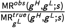 $ \frac {\mathrm {MR}^{obs}(g^H, g^L;s)}{\mathrm {MR}^{true}_{g^L}(g^H, g^L;s)}$
is increasing in
 $v_{g^H}(g^H)$
. Therefore, it takes the maximum value when
 $v_{g^H}(g^H) = 1$
.
 $$ \begin{align*} \frac{\mathrm{MR}^{obs}(g^H, g^L;s)}{\mathrm{MR}^{true}_{g^L}(g^H, g^L;s)} & \leq \frac{ \Gamma (g^H) \times \mathrm{MR}_{UY}(g^H,s)}{\Gamma (g^H) + \mathrm{MR}_{UY}(g^H,s) - 1}\\ & \leq \frac{ \mathrm{RR}_{GU} \times \mathrm{MR}_{UY}}{ \mathrm{RR}_{GU} + \mathrm{MR}_{UY} - 1} \end{align*} $$
where the second inequality comes from Lemma A.2 in Ding and VanderWeele (Reference Ding and VanderWeele2016) and
 $\Gamma (g^H) \leq \mathrm {RR}_{GU}, \mathrm {MR}_{UY} = {max}_{g,s} \mathrm {MR}_{UY}(g,s)$
.
From Lemma A.1 in Ding and VanderWeele (Reference Ding and VanderWeele2016), when
 $\Gamma (g^H) \leq 1$
,
 $ \frac {\mathrm {MR}^{obs}(g^H, g^L;s)}{\mathrm {MR}^{true}_{g^L}(g^H, g^L;s)}$
is nonincreasing in
 $v_{g^H}(g^H)$
. Therefore, it takes the maximum value at
 $v_{g^H}(g^H) = 0$
.
 $$ \begin{align*}\frac{\mathrm{MR}^{obs}(g^H, g^L;s)}{\mathrm{MR}^{true}_{g^L}(g^H, g^L;s)} \leq 1 \leq \frac{ \mathrm{RR}_{GU} \times \mathrm{MR}_{UY}}{ \mathrm{RR}_{GU} + \mathrm{MR}_{UY} - 1}\end{align*} $$
where the second inequality comes from Lemma A.2 in Ding and VanderWeele (Reference Ding and VanderWeele2016) and
 $ \mathrm {RR}_{GU} \geq 1 , \mathrm {MR}_{UY} \geq 1$
.
Hence, we obtain the desired result.
 $$ \begin{align*} \frac{\mathrm{MR}^{obs}(g^H, g^L;s)}{\mathrm{MR}^{true}_{g^L}(g^H, g^L;s)} \leq \frac{ \mathrm{RR}_{GU} \times \mathrm{MR}_{UY}}{ \mathrm{RR}_{GU} + \mathrm{MR}_{UY} - 1}. \end{align*} $$
Similar derivations apply to the other three inequalities. □
Proof of the theorem
For notational simplicity, we use the following representation.
 $$ \begin{align*} m(d,g; s) & \equiv \frac{1}{N} \sum_{i: S_i=s} \mathbb{E}[Y_i \mid T_i=d, G_i = g]\\ & = \frac{1}{N} \sum_{i: S_i=s} \frac{\sum_{u \in \Delta_s^u} \Pr(T_i=d, G_i=g, U_i=u) Y_i(d, g, u)}{\Pr(T_i=d, G_i=g)}\\ & = \frac{1}{N} \sum_{i: S_i=s} \sum_{u \in \Delta_s^u} \Pr(U_i=u \mid T_i=d, G_i=g) Y_i(d, g, u)\\ & = \sum_{u \in \Delta_s^u} \biggl\{ \frac{1}{N} \sum_{i: S_i=s} Y_i(d, g, u) \biggr\} \Pr(U_i=u \mid T_i=d, G_i=g)\\ & = \sum_{u \in \Delta_s^u} r_g(u) \Pr(U_i=u \mid T_i=d, G_i=g). \end{align*} $$
We want to show that, for
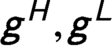 $g^H, g^L$
,
 $$ \begin{align*} \frac{m(d,g^H;s)}{B} - B \times m(d, g^L; s) \ \leq \ \frac{1}{N} \sum_{i: S_i=s} \tau_i(g^H, g^L; d) \ \leq B \times m(d,g^H;s) - \frac{m(d, g^L; s)}{B}. \end{align*} $$
Because this implies the desired result.
 $$ \begin{align*} & \frac{m(d,g^H;s)}{B} - B \times m(d, g^L; s) \ \leq \ \frac{1}{N} \sum_{i: S_i=s} \tau_i(g^H, g^L; d) \ \leq B \times m(d,g^H;s) - \frac{m(d, g^L; s)}{B} \\ & \Leftrightarrow \left\{ \begin{array}{ll} \sum_{s \in \mathcal{S}} \biggl\{ \frac{m(d,g;s)}{B} - B \times m(d, g^L; s) \biggr\} \ \leq \ \sum_{s \in \mathcal{S}}\biggl\{\frac{1}{N} \sum_{i: S_i=s} \tau_i(g^H, g^L; d) \biggr\} \\ \sum_{s \in \mathcal{S}}\biggl\{\frac{1}{N} \sum_{i: S_i=s} \tau_i(g^H, g^L; d) \biggr\} \ \leq \ \sum_{s \in \mathcal{S}} \biggl\{ B \times m(d,g^H;s) - \frac{m(d, g^L; s)}{B} \biggr\} \end{array} \right.\\ & \Leftrightarrow \frac{\mathbb{E}[\hat{m}(d,g^H)]}{B} - B \times \mathbb{E}[\hat{m}(d, g^L)] \ \leq \ \tau(g^H, g^L; d) \ \leq B \times \mathbb{E}[\hat{m}(d,g^H)] - \frac{\mathbb{E}[\hat{m}(d, g^L)]}{B}. \end{align*} $$
First, using Lemma 1,
 $$ \begin{align*} & \frac{m(d, g^H; s)}{ \sum_{u \in \Delta_s^u} r_{g^H}(u) \Pr(U_i=u \mid T_i=d, G_i=g^L)}\\ & = \frac{ \sum_{u \in \Delta_s^u} r_{g^H}(u) \Pr(U_i=u \mid T_i=d, G_i=g^H)} {\sum_{u \in \Delta_s^u} r_{g^H}(u) \Pr(U_i=u \mid T_i=d, G_i=g^L)}\\ & = \frac{ \sum_{u \in \Delta_s^u} r_{g^H}(u) \Pr(U_i=u \mid T_i=d, G_i=g^H)} {\sum_{u \in \Delta_s^u} r_{g^L} (u) \Pr(U_i=u \mid T_i=d, G_i=g^L)} \ \times \frac{\sum_{u \in \Delta_s^u} r_{g^L}(u) \Pr(U_i=u \mid T_i=d, G_i=g^L)}{\sum_{u \in \Delta_s^u} r_{g^H}(u) \Pr(U_i=u \mid T_i=d, G_i=g^L)}\\ & = \frac{MR^{obs}(g^H, g^L; s)}{MR^{true}_{g^L}(g^H, g^L; s)} \leq B \end{align*} $$
where the final equality follows from the lemma. Therefore,
 $$ \begin{align} \frac{m(d, g^H; s)}{B} \ \leq \ \sum_{u \in \Delta_s^u} r_{g^H}(u) \Pr(U_i=u \mid T_i=d, G_i=g^L). \end{align} $$
Also, since
 $B \geq 1$
,
 $$ \begin{align} \sum_{u \in \Delta_s^u} r_{g^L} (U) \Pr(U_i=u \mid T_i=d, G_i=g^L) \ = m(d, g^L; s) \ \leq \ B \times m(d, g^L; s). \end{align} $$
Finally, taking Equations (A5) and (A6) together,
 $$ \begin{align*} & \frac{m(d, g^H; s)}{B} - B \times m(d, g^L; s) \\ & \leq \sum_{u \in \Delta_s^u} r_{g^H}(u) \Pr(U_i=u \mid T_i=d, G_i = g^L) - \sum_{u \in \Delta_s^u} r_{g^L}(u) \Pr(U_i=u \mid T_i=d, G_i = g^L)\\ & = \sum_{u \in \Delta_s^u} \{r_{g^H}(u) - r_{g^L}(u)\} \Pr(U_i=u \mid T_i=d, G_i = g^L)\\ & = \frac{1}{N} \sum_{i: S_i=s} \sum_{u \in \Delta_s^u} \{Y_i(d, g^H,u) - Y_i(d, g^L, u)\} \Pr(U_i=u \mid T_i=d, G_i = g^L) \\ & = \frac{1}{N} \sum_{i: S_i=s} \tau_i(g^H, g^L; d). \end{align*} $$
Similarly, we want to prove
 $$ \begin{align*} & \frac{1}{N} \sum_{i: S_i=s} \tau_i(g^H, g^L; d) \leq B \times m(d, g^H; s) - \frac{m(d, g^L; s)}{B}. \end{align*} $$
First, since
 $B \geq 1$
,
 $$ \begin{align} \frac{m(d, g^L; s)}{B} \ \leq \ m(d, g^L; s) \ = \ \sum_{u \in \Delta_s^u} r_{g^L}(u) \Pr(U_i=u \mid T_i=d, G_i=g^L). \end{align} $$
Then, using Lemma 1,
 $$ \begin{align*} & \frac{\sum_{u \in \Delta_s^u} r_{g^H}(u) \Pr(U_i=u \mid T_i=d,G_i=g^L)}{m(d, g^H; s)}\\ & = \frac{ \sum_{u \in \Delta_s^u} r_{g^H}(u) \Pr(U_i=u \mid T_i=d, G_i=g^L)}{\sum_{u \in \Delta_s^u} r_{g^H}(u) \Pr(U_i=u \mid T_i=d,G_i=g^H)}\\ & = \hspace{-0.1in}\frac{\sum_{u \in \Delta_s^u} r_{g^H}(u) \Pr(U_i=u \mid T_i=d, G_i=g^L)} {\sum_{u \in \Delta_s^u} r_{g^L} (u) \Pr(U_i=u \mid T_i=d, G_i=g^L)} \times \frac{\sum_{u \in \Delta_s^u} r_{g^L}(u) \Pr(U_i=u \mid T_i=d, G_i=g^L)}{ \sum_{u \in \Delta_s^u} r_{g^H}(U) \Pr(U_i=u \mid T_i=d, G_i=g^H)}\\ & = \frac{MR^{obs} (g^L, g^H; s)}{MR^{true}_{g^L}(g^L, g^H; s)} \leq B. \end{align*} $$
Therefore, we have
 $$ \begin{align} \sum_{u \in \Delta_s^u} r_{g^H} (U) \Pr(U_i=u \mid T_i=d, G_i=g^L) \ \leq \ B \times m(d, g^H; s). \end{align} $$
Finally, taking Equations (A7) and (A8) together,
 $$ \begin{align*} & B \times m(d, g^H; s) - \frac{m(d, g^L; s)}{B} \\ & \geq \sum_{u \in \Delta_s^u} r_{g^H}(u) \Pr(U_i=u \mid T_i=d, G_i = g^L) - \sum_{u \in \Delta_s^u} r_{g^L}(u) \Pr(U_i=u \mid T_i=d, G_i = g^L)\\ & = \sum_{u \in \Delta_s^u} \{r_{g^H}(u) - r_{g^L}(u)\} \Pr(U_i=u \mid T_i=d, G_i = g^L)\\ & = \frac{1}{N} \sum_{i: S_i=s} \sum_{u \in \Delta_s^u} \{Y_i(d, g^H,u) - Y_i(d, g^L, u)\} \Pr(U_i=u \mid T_i=d, G_i = g^L) \\ & = \frac{1}{N} \sum_{i: S_i=s} \tau_i(g^H, g^L; d). \end{align*} $$
Hence we have
 $$ \begin{align*} \frac{m(d,g^H;s)}{B} - B \times m(d, g^L; s) \ \leq \ \frac{1}{N} \sum_{i: S_i=s} \tau_i(g^H, g^L; d) \ \leq B \times m(d,g^H;s) - \frac{m(d, g^L; s)}{B}, \end{align*} $$
which completes the proof. □
Acknowledgments
I thank Alexander Coppock, Andrew Guess, and John Ternovski for providing me with data and answering my questions. I also thank Peter Aronow, Neal Beck, Forrest Crawford, Christian Fong, Erin Hartman, Zhichao Jiang, Marc Ratkovic, Cyrus Samii, Fredrik Sävje, Matthew Salganik, members of Imai research group, and participants of the seminars at Yale University and New York University for helpful comments. I am particularly grateful to Kosuke Imai, Brandon Stewart, Santiago Olivella, and Adeline Lo for their continuous encouragement and detailed comments. I thank the editor and two anonymous reviewers for providing me with valuable comments. The earlier draft of this article was entitled “Unbiased Estimation and Sensitivity Analysis for Network-Specific Spillover Effects: Application to An Online Network Experiment” (Egami Reference Egami2017).
Data Availability Statement
The replication materials are available as Egami (2020).
Supplementary Materials
To view supplementary material for this article, please visit http://dx.doi.org/10.1017/pan.2020.28.