Railroads constituted one of the most important technological breakthroughs of the nineteenth century, leading to a substantial upward shift in national economies' production functions worldwide. Attempts to measure their growth impact have given rise to one of the most famous debates in economic history, one of whose conclusions is the idea that their role was especially crucial in those countries which lacked an extensive system of waterways at the beginning of the railroad era, or whose geography put serious constraints on the development of water transport.1
See, among others, Fogel, Railroads, p. 31, and O'Brien, “Transport,” pp. 12–13.
See Fogel, “Notes,” pp. 2–5.
As may be observed in Table 1, the first social saving estimates, which were produced for highly developed countries such as the United States or the United Kingdom, were rather small, because those economies had relatively large endowments of inland waterways or coastal shipping opportunities at the beginning of the railroad era and, therefore, low prospects of reducing transport unit costs through the use of railroads. By contrast, when the same methodology was applied to less developed economies with fewer possibilities for cheap water transport, such as Spain in Europe or Mexico, Brazil, and Argentina in the Americas, the ratios between each country's social savings and GDP turned out to be much higher. The main alleged reason for that situation was the prominence that roads would have had in a counterfactual transport system without railroads in those countries, which would have increased substantially the unit savings in transport costs that were produced by the railroad system.

However, it is arguable to what extent such a general interpretation may be drawn from the direct comparison among a few social saving estimates that have been produced for rather distant points of time, and, in fact, railroad historians have been reluctant to accept its implications for some countries. In the Spanish case, for instance, some researchers have indicated that the hypothesis that the railroads had a considerable impact on economic growth, which might be inferred from the observation of Antonio Gómez Mendoza's social saving estimates in Table 1, is in conflict with other evidence, such as the low utilization of the network or the railroad companies' constant financial problems. According to some historians, it is difficult to understand why the Spanish railroad companies were unable to capture a larger share of the exceedingly high social savings of the railroad system. In that context, some authors have tried to reconcile all that apparently contradictory evidence.3
Keefer, for example, has indicated that the companies' low rates of return were the counterpart of high construction profits, because investors wanted to secure their returns earlier rather than later, due to the lack of credibility of the Spanish State regarding property rights. See Keefer, “Protection.”
See, especially, Tortella, Los orígenes, p. 169, and “Introducción,” pp. 250–53.
This article aims at reassessing the economic impact of the Spanish railroads from a new perspective, in order to shed some light on the ongoing debate on the topic. Instead of relying on the traditional social saving methodology, this research is based on the application of growth accounting techniques, which constitute the most usual way to evaluate the economic growth implications of new technology, and have been recently used by Nicholas Crafts to analyze the contribution of steam technology (railroads included) to British labor productivity growth between 1760 and 1910. Growth accounting addresses the general question “how much did the new technology contribute to productivity growth?” rather than the more specific question “how much faster was productivity growth as a result of the introduction of the new technology?” which is the actual objective of social saving analysis.5
Crafts, “Steam,” p. 340.
THE GROWTH ACCOUNTING METHOD
The most usual way to measure the global contribution of technological change to economic growth is the estimation of the so-called “Solow Residual,” on the basis of a typical Cobb-Duglas production function and competitive assumptions. The “Solow residual” (ΔA/A) was originally interpreted as the TFP growth provided by new technology, and is estimated from the following expression

where Y is total output, K denotes the services provided by the capital stock, L is the total number of hours worked, and sK and sL are the factor income shares of labor and capital, respectively.
Some recent research on the contribution of information and communication technologies to economic growth has been based on a generalization of expression 1, which aims at incorporating the hypothesis of endogenous innovation and embodied technological change. Stephen D. Oliner and Daniel E. Sichel, for instance, apply a disaggregated version of equation 1, in which different types of capital and different components of TFP growth are distinguished. This allows them to measure the impact of ICT on productivity, both through disembodied TFP growth and through the embodied capital-deepening effect of investment in ICT. Therefore, they transform expression 1 into

where Y is total output, L is the total number of hours worked, KICT and Ko are the services provided by capital stock in ICT and in other sectors, respectively, A is the TFP level in the sector indicated by the subscript (ICT and other), sL, sKICT and sKo are the factor income shares of labor, ICT capital and other capital, and φ and γ are the shares of ICT and other sectors' production in total output. Equation 2 may be modified in order to account for labor productivity growth

The contribution of a new technology to labor productivity growth may be approached by the sum of the last two terms of equation 3. In fact, this would be a lower bound estimate of the real impact of the new technology, as there may be spillovers from the sector under consideration to the rest of the economy. Unfortunately, growth accounting studies usually fail to quantify indirect TFP spillovers, due to the measurement difficulties involved.6
See Oliner and Sichel, “Information Technology,” pp. 16–20; and Crafts, “Steam,” pp. 339–340.
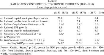
Table 2 displays Crafts's estimates of the contribution of the railroads to British labor productivity growth between 1830 and 1910, which are the result of the application of this measurement technique. As is usual in this kind of exercises, figures in the table exclude TFP spillovers. The main conclusion that may be drawn from Crafts's estimates is that the impact of railroads before 1850, although appreciable, did not transform the overall growth rate of the economy, due to the small size of the sector relative to GDP. Actually, their maximum contribution arrived in 1850–1870, when TFP growth achieved its highest rate and the railroad system was much larger. During those two decades, the railroads would have accounted for nearly 20 percent of British income per capita growth. The importance of the railroads would have decreased later on to much lower levels, as both the slowness of productivity growth in the sector and the low investment in the network made up for the higher share that the railroad output accounted for within the economy.

The application of this methodology to the Spanish railroads must face two main obstacles. The first one, which is shared with other research, is the difficulty of quantifying TFP spillovers from the railroads to the rest of the economy. The relevance of spillovers is a non-negligible potential source of downward bias in the estimation of the contribution of railroads to economic growth, whose absence must be kept in mind in the interpretation of the results. The second problem regards the estimation of the TFP term in expression 3. In his analysis of the British case, Crafts uses the available indices of TFP growth in the railroad sector, obtained through the application of conventional index number techniques. This procedure cannot be applied in the Spanish case for two reasons. Firstly, there is not enough information available on some of the series that are necessary to directly estimate TFP growth indices in the Spanish railroads, such as the number of workers or the companies' yearly coal consumption. And, secondly, an index of TFP growth in the railroad sector cannot be assumed to include the whole TFP impact of Spanish railroads. Whereas the first British railroads had no great cost advantage over their main competitor (i.e., water transportation) when they were established, the first Spanish railroad services were considerably cheaper than the alternative modes they displaced (mainly traditional overland transportation). Therefore, an account of the whole TFP effects of the Spanish railroads should not only include TFP improvements within the railroad sector itself (as in Britain) but also those TFP gains that were associated with the shift from old forms of transportation to the railroads.
In this context, the TFP term in expression 3 may be approached in two steps. On the one hand, the rate of TFP growth within the railroad sector may be calculated on the basis of the econometric estimation of a cost function for the Spanish railroad companies. The basic form of such function is

where C is cost, Y is the vector of outputs, W is the vector of input prices, T is time, and F represents certain characteristics of each company's network, such as the average haul or load. The estimation of this function allows decomposing changes in railroad costs between its different sources: price variations (through the coefficients of W), growth of output (through the coefficients of Y), technical and organizational progress (through the coefficient of T), and changes in network characteristics. On the basis of the dual theory of production, the estimation of this function also allows calculating the growth rate of TFP in the Spanish railroads as the equiproportionate yearly increase in output with input fixed.
The growth rates of TFP obtained in this way may be compared with the British equivalent figures to analyze differences in productivity growth between both railroad systems. However, as has been indicated, they would not account for the whole TFP impact of the Spanish railroads, because they would exclude the TFP gains resulting from the substitution among different transport modes. These might be approached instead on the basis of the available social saving estimates for the Spanish railroad system. Social savings are usually calculated as

where PFC and PALT are, respectively, the price of railroad and counterfactual transport, and QFC is the railroad transport output in the reference year. This expression was interpreted by Fogel as a measure of the resources released by the railroad technology.
7Fogel, “Notes,” p. 5.
Metzer, “Railroads,” p. 68; Jara-Díaz, “Relation.”
As Crafts has recently stressed, the price dual measure of TFP allows considering such gain in real income as equivalent to the increase in TFP provided by the railroads. In a country such as Britain, where railroads were only introduced at the point where they could offer transport at the same cost as water transportation, it should actually be equivalent to TFP gains in the railroad sector itself.9
Crafts, “Social savings,” p. 6.
Actually, although small, there was also some potential transport cost reduction in Britain coming from the substitution of the railroads for alternative transport modes; see Hawke, Railways. Therefore, an account of the growth contribution of the British railroads such as that in Table 2, which is just based on the increase in TFP within the railroad sector, would contain certain downward bias associated with the exclusion of those gains, which must be kept in mind in the comparison between the British and the Spanish cases.
SPANISH RAILROAD TFP GROWTH: THE COST FUNCTION APPROACH
There is a well-established tradition of using cost function analysis to estimate the structure of railroad production and the rate of growth of TFP in railroad systems.
11See a survey of this type of analysis in Oum, Waters, and Yu, “Survey.”

This is equivalent to estimate TFP growth as the product of two factors: the rate of growth of technical change (i.e., the rate at which all inputs can be decreased over time with outputs held fixed; −εct in expression 6), and the level of returns to scale in the system (i.e., the proportional increase in all outputs that results from a proportional increase in all inputs with time fixed; (

) in expression 6).
If the firm is assumed not to minimize cost with respect to all inputs but only to a subset of variable factors, conditional on the level of the remaining (quasi-fixed) inputs, then the total cost function does not exist, and the variable cost function provides all the information required to infer the structure of production. In variable cost analysis, if quasi-fixed inputs are represented by network length N (as is usual in those cases, such as the current research, in which the necessary information on each company's assets is incomplete) comparative statics analysis implies the following corrections for the formulae of technical change and returns to scale:
12A discussion on these aspects, as well as the mathematical developments that yield these formulae, may be seen in Caves, Christensen, and Swanson, “Productivity Growth,” pp. 995–96.


Returns to scale calculated as in expression 8 are most often denominated “returns to traffic density,” because they reflect the relationship between inputs and outputs with the rail network held fixed. They constitute, therefore, an indicator of the opportunities to reduce average cost through increased use of the network, on the basis of potential economies in the use of trains, labor, and equipment.13
On this subject see Keaton, “Economies,” p. 212.
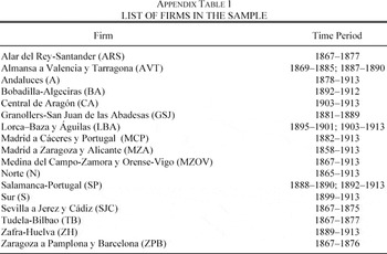
As may be readily inferred, the product of technical change (expression 7) and returns to density (expression 8), defined in terms of variable cost function elasticities, still yields expression 6 for the rate of growth of TFP. This section presents estimates of TFP growth and its two underlying factors (technical change and returns to density) for the Spanish railroads between 1858 and 1913, on the basis of a variable translog cost function, estimated for an unbalanced panel of 17 broad-gauge companies with a network longer than 100 km (accounting on average for 65 percent of the whole railroad network of the country). The specification of the function and the complete estimation results may be seen in Appendix 1.
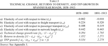
The estimated coefficients of the variable cost function allow calculating partial elasticities of cost with respect to the explanatory variables at the sample mean, as well as estimates of the growth rate of technological change, returns to density and TFP growth, for two time spans: 1858–1890 and 1891–1913. The distinction between these two periods responds to the incorporation of a trend dummy in the specification of the function, whose break point (1890) has been established on the basis of the Akaike information criterion. All estimates are displayed in Table 3. According to the table, the yearly rate of TFP growth in the Spanish railroad system was 0.53 percent between 1858 and 1890 and 2.28 percent between 1891 and 1913. These growth rates are within the range of those estimated for contemporary railroads.14
See Oum, Waters, and Yu, “Survey,” p. 29.

As has been pointed out, TFP growth may be considered as the product of the rate of growth of technical change and returns to traffic density. Regarding the latter, estimates in Table 3 indicate that Spanish railroads could benefit from substantial increasing returns to density during the whole period (at a level of 1.4 / 1.3). In other words, there were significant prospects of increasing productivity through the growth of output. Because the density of use of the Spanish railroad network grew more than three-fold between 1860 and the outbreak of the First World War, the railroad companies could indeed take advantage of that feature to increase their TFP throughout the period.15
For the sources of information on the output of the Spanish railroads, see Appendix 1.
The potential influence of returns to density on productivity was similar both before and after 1890, because neither the level of returns to density nor the growth rate of density itself experienced major changes between the two subperiods under consideration. By contrast, the growth rate of technical change substantially increased after 1890, from 0.4 to 1.8 percent per year, and this change fully explains the acceleration in TFP growth from that year onwards. This increase is somehow surprising, as technology in the railroad sector did not suffer major alterations between the 1870s and the general adoption of electric power. However, there were some opportunities for efficiency growth through the companies' agreements to share infrastructure or rolling stock, the use of steel instead of iron rails, and increases in locomotive power or in car capacity.16
See, for instance, Fishlow, “Productivity,” pp. 634–42.
For the increase in locomotive power, see Comín, Martín Aceña, Muñoz et al., 150 años, vol. 1, pp. 102–06. For companies' mergers and takeovers, which explain the increasing shared utilization of infrastructure and rolling stock, see Tedde, “La expansión,” pp. 277–79.
SPANISH RAILROADS TFP GROWTH: THE SOCIAL SAVING APPROACH
The TFP gains provided by the Spanish railroad system may also be approached on the basis of the available social saving estimates. As has been pointed out, as far as the social savings represent the total direct gain in real income obtained from reducing resource costs in transportation, they will be equivalent to the total increase in TFP provided by the railroads to the economy. Accordingly, estimates of TFP gains based on the social savings will not only account for TFP growth in the railroad sector (as the figures that have been presented in the previous section) but also for the productivity effect of the shift from alternative transport modes to the railroads.
Actually, the equivalence between the social savings and TFP growth was already used by James Foreman-Peck to estimate the social savings of the English and Welsh railroads in 1890 on the basis of Gary Hawke's figure for 1865 and an index of railroad TFP growth.18
Foreman-Peck, “Railways,” pp. 76–77.
See Crafts, “Social Savings,” p. 6.
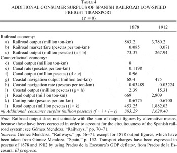
In the case of low-speed freight transport (livestock excluded), all the necessary information to estimate the equivalent variation consumer surplus created by the Spanish railroads is provided by Gómez Mendoza in his social saving exercise. This author offers output and price figures for railroad and alternative transport means both for 1878 and 1912.20
On these issues, see Gómez Mendoza, “Railways,” pp. 50–64.
Figures in Table 4 are upward biased because they do not allow for the rerouting of transport flows. These would probably have been relevant in the Spanish economy, because railroad routes might often be replaced by combinations of road transport and coastal navigation that were longer in distance, but cheaper than the direct road connection. For instance, before the railroad era, the wheat produced in Northern Castile was shipped to Catalonia not directly by road, but by boat from the Northern coast, circumventing the Peninsula, and this indirect route was likely to have been used again in a counterfactual economy without railroads; see, for instance, Garrabou and Sanz, “La agricultura española,” p. 49. However, the lack of precise information on the origin and destination of the actual railroad flows prevents the estimation of the magnitude of the bias associated with this aspect and Gómez Mendoza provides some evidence that interseas coastal trade shipment would have played a minor role in a counterfactual economy without railways; see Gómez Mendoza, “Railways,” p. 54.

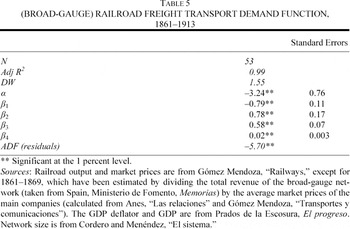
These figures must be corrected by the elasticity of transport demand, in order to eliminate their upward bias. As in similar research for other countries, the following transport demand function has been estimated for the period 1861–1913
22See, for example, Coatsworth, “Indispensable Railroads,” p. 951; Summerhill, Order, p. 94; and Ramírez, “Los ferrocarriles,” p. 100.

where Q is the railroad freight output, P is the average market price of railroad freight transport (expressed in constant pesetas of 1861) and N is the size of the railroad network. The unit root test analysis of the variables that appear in the function is shown and discussed in Appendix 1, and the results of the OLS estimation of the function are displayed in Table 5. The estimation output is actually the error correction vector of a cointegration model, because the residuals of the equation appear to be stationary. The price coefficient indicates an elasticity of demand of −0.79. According to this estimate, the “true” unbiased value of the additional consumer surplus provided by railroad low-speed freight transport was 163.68 million pesetas in 1878 (i.e., 43 percent of the upward biased estimate in Table 4) and 649.29 million pesetas in 1912 (i.e., 40 percent of the upward biased estimate).
23The ratio between the biased and unbiased estimates of additional consumer surplus is given by [(ϕ1 + ε − 1) / (1 + ε)(ϕ − 1)], where ε is the elasticity of transport demand and ε is the ratio between counterfactual and railroad transport prices; see Fogel, “Notes,” pp. 10–11.

A similar estimation may be carried out in the case of passenger traffic. Gómez Mendoza's social saving figures did not include passenger transport, because he considered it as a completely new commodity which, for the most part, would never have taken place without the advent of the railroads.24
Gómez Mendoza, “Railways,” p. 26.
Gómez Mendoza, “Transportes,” p. 477.
Madrazo, El sistema, p. 534.
Figure coming from Spain, Ministerio de Fomento, Memoria(s).
See Coatsworth, “Indispensable railroads,” pp. 943–44; and Summerhill, Order, pp. 112–13.
Table 6 presents an estimate of the (upward biased) additional consumer surplus created by Spanish first- and second-class passenger railroad transport in 1878 and 1912, which includes both the savings in transport unit costs and the working time saved thanks to higher speed. I have assumed first- and second-class travelers to be among the highest-income social groups, and have valued their travel time at twice the hourly wage of skilled industrial workers.29
A similar procedure is followed by Summerhill, Order, p. 113.
See Summerhill, Order, pp. 116–22; Metzer, Some Economic Aspects, pp. 60–62; and Coatsworth, “Indispensable Railroads,” p. 945. There is, however, a great deal of uncertainty on the reasons for journeys in Spanish passenger transport.

As in the case of freight, figures in Table 6 must be corrected for the price-elasticity of demand. This is difficult to estimate in the Spanish case, given the lack of information about the distribution of passenger transport between classes for a large part of the period under study. Research for other countries has assumed an elasticity of −1 for transport demand, and this figure is consistent with the information available for one of the largest Spanish companies (MZA).31
For the United States, Boyd and Walton, “Social Savings,” pp. 247–50; and, for Russia, Metzer, Some Economic Aspects, p. 73. A preliminary time-series estimation of first- and second-class passenger transport demand elasticity for the company MZA in 1883–1912 offers a result of –0.82. The details of this estimation are available upon request.
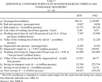
Table 7 presents the additional consumer surplus associated with third-class passenger transport under the assumption of a completely inelastic demand, on the basis of the same information as the first and second classes. The only difference is the valuation of time savings, which is based in this case on the hourly wage of skilled industrial workers.32
Summerhill, Order, p. 117, uses, for lower-class passengers, a combination of the wages of “farm workers” and “skilled manufacturing workers.” Other authors use the wage of “railroad workers” or “manufacturing workers,” without specifying professional rank; see Coatsworth, “Indispensable Railroads,” p. 945; and Boyd and Walton, “Social Savings,” p. 245.
See, for instance, Hausman, “Valuation.”

Other sorts of freight transport (essentially high-speed freight) cannot be analyzed in the same way, because neither the official statistics nor the companies' accounts provide enough information to estimate output or market prices for the whole network. These traffic categories accounted for a non-negligible share of the total revenues of the railroad companies (7.6 percent in 1878 and 10.3 percent in 1912) and, therefore, their absence introduces certain downward bias in the global additional consumer surplus estimates. This bias, however, is probably small. Because, as in the case of third-class passenger transport, most of that traffic might be considered as a completely new commodity, its contribution to the additional consumer surplus may be expected to be rather low.
Once the assumption of a price-inelastic transport demand has been removed, the additional consumer surplus figures must also be corrected to account for the presence of idle resources in the economy and the lack of competition in the railroad industry. Regarding the first issue, Gómez Mendoza provided alternative estimates of the railroad social saving for freight in 1878 that took into account the presence in the Spanish economy of a pool of underemployed peasants, which could have provided road transport services in the absence of the railroad system. In those estimates, the opportunity cost of road transport in the counterfactual economy is much lower than the actual market price (0.082 pesetas of 1878 per ton-km). The replacement of PALT by that opportunity cost for two-fifths of all freight transported by road in the counterfactual economy (i.e., for freight transported during the off-peak months of the agricultural working year) decreases the (unbiased) additional consumer surplus for low-speed freight transport by 24.37 percent in 1878 and 21.61 percent in 1912.34
For the estimation of the opportunity cost figure and the two-fifths parameter, see Gómez Mendoza, “Railways,” pp. 80–90.
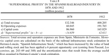
Secondly, in the estimation of the total resource savings provided by the railroads, it is necessary to account for the lack of competition in the railroad industry or, in other words, for the presence of supernormal profits in the sector.35
See McClelland, “Social Rates of Return,” and Crafts “Social Savings,” p. 7, footnote 2.
See, for instance, Tortella, “Introducción,” p. 250; Comín, Martín Aceña, Muñoz et al., 150 años, Vol. 1, p. 144; or Keefer, “Protection,” pp. 174–75.
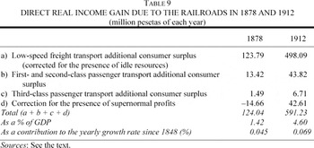
Table 8 presents a calculation of the level of “supernormal profits” in the Spanish railroad industry in 1878 and 1912. For 1878, it confirms the impression of the sector's highly unfavorable financial situation during the first decades of the railroad era whereas, in the case of 1912, it reflects the effects of increasing efficiency and use of the network, which finally allowed the system to obtain positive supernormal returns in the eve of First World War. Figures in Table 8 are combined in Table 9 with the previous outcomes of the estimation of additional consumer surplus for different kinds of traffic. The sum of all these figures may be considered as a measure of the entire direct real income gain due to the railroads, which is expressed as a contribution to the annual rate of economic growth in the last row of the table.


THE CONTRIBUTION OF RAILROADS TO SPANISH ECONOMIC GROWTH
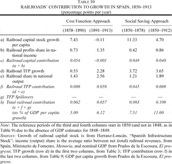
Table 10 reports the contribution of railroads to Spanish economic growth, as results from the different TFP estimates that have been presented in the previous sections. Rows a to c display the railroad capital deepening contribution to growth in different periods, which is based on the most recent estimates of Spanish railroad capital stock. Rows d to f, in turn, present the TFP growth contribution. In the first two columns, the TFP growth rates that were obtained from the estimation of the railroad cost function are included in row d and multiplied by the share of railroad output within GDP, in order to get figures of total TFP contribution. In the last two columns, the global TFP contribution that was estimated in the previous section on the basis of the social savings is included in row f and divided by the railroad output share to obtain an implicit TFP growth rate (row d), which includes the productivity effects of the substitution among transport modes.
Although the periods that are distinguished in the table are not strictly comparable with those considered by Crafts in his analysis of the British case (Table 2), it is possible to identify two features that the Spanish railroad system shared with the British one. Firstly, in both countries the growth rates of the railroad capital stock per person (row a) decreased as time went by and as the construction of the network gradually arrived to its virtual completion. The railroad stock per capita grew at extremely high rates during the first few years of the railroad era in both cases (22.8 percent in Britain in 1830–1850, and 22 percent in Spain in 1850–1866) and slowed down thereafter to much lower levels. The decrease was even more marked in Spain than in Britain, because the limited growth of the Spanish railroad network after the 1890s resulted in a negative rate in per capita terms since 1897. As a consequence of this evolution of the capital stock, during the first years of the railroad era most of the growth contribution of the railroad system was associated in both countries to capital deepening effects, whereas, as time went by and the growth of the railroad capital stock tended to stagnate, these effects became negligible and the TFP contribution gained increasing relevance.

Secondly, Tables 2 and 10 show that the participation of the railroad sector within the economy (rows b and e) increased steeply in both countries as time went by. In the Spanish case, for instance, the share of the railroads within national income increased eleven-fold between 1859 and 1912, and the importance of the sector within gross output experienced an eight-fold growth during the same period.
Regarding the growth rates of TFP (row d), similarities between both countries are less patent. In Britain, this variable showed an inverted-U pattern, reaching its maximum (3.5 percent per year) during the period 1850–1870 and staying at much lower levels both in 1830–1850 (1.9 percent) and in 1870–1910 (1 percent). In the Spanish case, if only productivity improvements within the railroad sector are considered, the growth rate of TFP appears to have been extremely slow until 1890 (0.5 percent), and to have accelerated substantially thereafter up to a level of 2.3 percent per year. By contrast, if the productivity gains that resulted from the substitution of the railroads for alternative transport means are also included in the estimation, the Spanish implicit growth rate of TFP (3.7 percent) appears to have been higher than the British maximum rate during the whole period under study. In addition, the comparison between this rate and those coming from the Spanish railroad cost function would imply that, before 1890, most railroad productivity gains were the result of the substitution among transport modes whereas, after that year, more than 50 percent of the TFP contribution came instead from efficiency improvements within the railroad system and from increasing density of use of the network.
The last two rows of Table 10 present estimates of the whole direct contribution of railroads to Spanish economic growth between the mid nineteenth century and the First World War. According to those figures, if the shift from alternative transport modes to the railroads is not considered, the direct economic impact of railroads amounted to 0.06 percentage points of growth per year (or, in relative terms, 5.0 to 6.1 percent of Spanish income per capita growth). By contrast, if the effects of the substitution among different transport modes are included, the global contribution was 0.11 percentage points per year (or 11 percent of income per capita growth). Although these are significant contributions for a single sector, they are not higher than the British equivalent figure, which amounted, on average, to 0.14 percentage points per year between 1830 and 1910 (or 12 percent of income per capita growth).37
See Table 2. Actually, the Spanish disadvantage would appear even larger if the (small) TFP gains associated to the substitution of the British railroads for alternative transport modes were also accounted for in the British estimates (see footnote 10).
Figures in Tables 2 and 10 clearly show that the Spanish disadvantage was not the outcome of a slower growth rate of the capital stock or a stagnant TFP. On the contrary, the growth of railroad capital was to some extent comparable among both countries, and the growth rate of TFP seems to have been higher in Spain than in Britain. The main reason for the Spanish disadvantage was the fact that, at similar capital stock and TFP growth rates, the shares of the Spanish railroads within national income (row b) and output (row e) were always lower than the British ones. Therefore, the potential benefits coming from the huge cost difference between the railroads and the alternative transport means were overcome in Spain by the minor role played by railroad transport in the economy. In sum, the direct contribution of the railroads to economic growth was not higher in Spain, whose geography put serious constraints on the development of water transportation, than in Britain, which could use it extensively before the advent of the railroads. To some extent, this result is in conflict with the general considerations of the traditional social saving literature, and might be explained by the fact that a large share of the much less developed Spanish economy remained largely unaffected by the railroad system for a long time, a situation that could probably be also found in other peripheral economies (such as those of Mexico, Brazil, and Argentina) which had both low prospects for resorting to cheap water transport and relatively low levels of development during the railroad era.
Finally, however, it is necessary to recall that growth accounting figures in Tables 2 and 10 exclude TFP spillovers, due to the difficulty of quantifying them. The relevance of TFP spillovers from the railroads is a non-negligible potential source of downward biases in growth accounting estimates, but the extent to which their inclusion might reduce the distance between the growth contribution of the Spanish and British railroads remains mere conjecture. In this context, within a future research agenda on the economic role of railroads, the importance of TFP spillovers from the railroad system must be considered as one of the most crucial aspects to analyze.
CONCLUSION
This article has provided growth accounting estimates of the contribution of railroads to Spanish economic growth, offering new insights on the long debated topic of the role of railroads in Spain's industrialization. Spain has usually been included among those countries where the railroads were expected to exert a higher potential impact, due to the lack of an extensive water transport system at the beginning of the railroad era. That hypothesis was reinforced by the outcomes of the early social saving literature, but received strong criticisms by some historians, due to the low density of use and the bad financial situation of the Spanish railroad companies. In that context, growth accounting has provided a more complete and comparable assessment of the growth contribution of the Spanish railroads than the traditional social savings estimates.
The analysis carried out here shows that the TFP gains associated to the Spanish railroads were substantial before 1914, both through the shift from alternative transport means to the railroads and (especially since the last few years of the nineteenth century) through productivity improvements within the railroad system itself. However, in spite of those gains, the total direct impact of the Spanish railroads only accounted for 11 percent of income per capita growth, a percentage that was not higher, on average, than those estimated for the United Kingdom by Crafts. The main reason for this unexpected finding is the low importance of railroad transport within Spanish GDP, which prevented the resource savings provided by the substitution of the railroads for traditional overland transport, as well as the productivity gains that took place up to 1914, from having a more substantial impact on income per capita levels. In sum, the traditional hypothesis that the countries that gained most from the railroads were those where the share of freight taken off the roads and onto the railroad networks was higher, needs to be qualified on the basis of the different role that the railroads performed in each economy.
Appendix 1: Spanish Railroad Cost Function (1858–1913)
In order to estimate TFP growth in the Spanish railroad sector, I write the following generalized translog variable cost function

where Yi represents different outputs (ton-km and passenger-km), Wi represents prices of different inputs (labor, coal and iron), N is the network length, $T $is a time trend representing technological change, DT is the product of the time trend and a dummy that takes the value one for all years before a given t, and F is a set of individual firm dummies. The endogenous variable is each company's yearly variable cost. The model has been estimated for an unbalanced panel of 17 broad-gauge companies with a network longer than 100 km, which are listed in Appendix Table 1. Given the large number of parameters to estimate (60 with two outputs and three inputs), larger actually than the number of time observations, it has been necessary to incorporate additional restrictions in order to obtain relatively better defined coefficients. On the basis of the significance of the individual coefficients and the outcomes of the Akaike criterion, all coefficients of the products of input prices among them and with other variables have been assumed to be zero, as well as the coefficients of the products of output variables and network length and the products of the time trend and the time trend dummies with all other variables. This has reduced the number of parameters to estimate to 31. The Akaike criterion has also been used to set the trend dummy as equal to zero from 1891 onwards.

The data used in the estimation come from the following sources: a) Variable cost, output and network length of each company from Anes, “Relaciones,” pp. 508–09; Anuario, various dates; Cambó, Elementos, vol. 2, pp. 94–98; Compañía de los Ferrocarriles de Madrid a Zaragoza y Alicante (MZA), Memoria; Gómez Mendoza, “Transportes y comunicaciones,” pp. 293–94; Spain, Ministerio de Fomento, Memoria; and Spain, Ministerio de Obras Públicas, Plan General, vol. 4, pp. 12–65. Each company's output before 1897, when not available, has been estimated by assuming similar hauls to later periods. b) Factor prices come from Anes, “Relaciones,” p. 450; Carreras, “La industria,” pp. 216–26; Coll and Sudrià, El carbón; Compañía de los Caminos de Hierro del Norte de España, Compañía; and Reher and Ballesteros, “Precios.”
Appendix Table 2 displays the outcomes of the estimation of the model. Estimates in the table are feasible generalized least squares, robust to the presence of autocorrelation and panel heteroskedasticity.

Appendix 2: Transport Demand Function (Unit Root Tests)
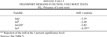
The series included in the transport demand function (equation 10) have been applied the Dickey-Fuller unit root test in order to know their level of integrability. The results of the test are shown in Appendix Table 3. All series appear to be I(1), with the exception of lnN, for which the null of presence of a unit root tends to be rejected, although this result depends on the specification of the test. The ambiguity of this outcome result gives some support to the consideration of this variable as a “near-unit-root” process, which are often recommended to be treated as unit root processes, given the low power of the available tests (see, for instance, Granger, “What are we Learning about the Long Run?” pp. 309–10; and Doornik, Hendry, and Nielsen, “Inference,” p. 536). This choice has been adopted here because it allows working with the series in levels and keeping all the information that they contain. In addition, it makes possible to obtain elasticity figures that are comparable to other countries' and may be used to correct the bias of figures in Table 4.

I thank the Bank of Spain and the Spanish Ministry of Education Grant SEJ2005-02498 for financial support. I gratefully acknowledge comments by participants in seminars at the London School of Economics, UC-Berkeley, the Universities of Oxford, Barcelona, Valencia, Zaragoza, Carlos III and Pompeu Fabra, and at the 5th European Historical Economics Society Conference (Madrid, July 2003). I am particularly indebted to Dudley Baines, Nicholas Crafts, Antonio Gómez Mendoza, Patrick O'Brien, Pere Pascual, Leandro Prados de la Escosura, Max-Stephan Schulze, Carles Sudrià, William Summerhill, Daniel A. Tirado, and three anonymous referees. This implies no responsibility on their part for the shortcomings that may remain in the article.