



1. Introduction
Shock wave/turbulent boundary layer interaction (STBLI) occurs widely in the internal and external flows of high-speed aircraft. It can generate local strong pressure fluctuations, which may lead to structural vibration, fatigue or even structural failure (Dolling Reference Dolling2001; Gaitonde Reference Gaitonde2015), seriously impacting the aerodynamic performance and structural safety of the aircraft. Therefore, investigating the physical characteristics of pressure fluctuations in STBLI is crucial for the design and optimisation of high-speed aircraft.
In STBLI, the adverse pressure gradient induced by strong shock waves causes significant flow deceleration in the boundary layer and flow separation (Delery Reference Delery1985; Wang et al. Reference Wang, Wang and Zhao2016, Reference Wang, Wang, Sun, Yang, Zhao and Hu2019), thereby complicating the unsteady characteristics of the pressure fluctuations. This unsteady behaviour has remained at the forefront of STBLI research for decades (Dupont et al. Reference Dupont, Haddad and Debieve2006; Wu & Martin Reference Wu and Martin2007; Ringuette et al. Reference Ringuette, Bookey, Wyckham and Smits2009), with numerous investigations dedicated to unravelling its origins yet yielding no universally accepted explanation. These can be summarised into three main categories: (i) the upstream mechanism (Beresh et al. Reference Beresh, Clemens and Dolling2002; Ganapathisubramani et al. 2007, Reference Ganapathisubramani, Clemens and Dolling2009; Vanstone & Clemens Reference Vanstone and Clemens2019); (ii) the downstream mechanism (Wu & Martin Reference Wu and Martin2008; Piponniau et al. Reference Piponniau, Dussauge, Debieve and Dupont2009; Priebe & Martín Reference Priebe and Martín2012; Ji et al. Reference Ji, Jiang, Zhu, Yang and Xia2025); (iii) the combined effects of both upstream and downstream mechanisms (Souverein et al. Reference Souverein, Dupont, Debieve, Dussauge, van Oudheusden and Scarano2010; Clemens & Narayanaswamy Reference Clemens and Narayanaswamy2014; Martin et al. Reference Martin, Priebe and Helm2016). Ganapathisubramani et al. (Reference Ganapathisubramani, Clemens and Dolling2007, Reference Ganapathisubramani, Clemens and Dolling2009) conducted numerical simulations and experimental research, and concluded that the superstructures in the turbulent boundary layer, which are 30–40 times the thickness of the boundary layer, are the main cause of low-frequency oscillations, i.e. the upstream mechanism. Priebe & Martín (Reference Priebe and Martín2012) found that the unsteady motion of the shock wave is related to the ‘breathing’ of the separation bubble and the oscillation of the shear layer, but has a very weak correlation with the upstream boundary layer, which provides evidence for the downstream mechanism. In addition, Martin et al. (Reference Martin, Priebe and Helm2016) found that the Görtler vortices are modulated by the disturbances in the upstream boundary layer, and in turn affect the unsteady characteristics of the separated flow, ultimately leading to the simultaneous operation of the upstream/downstream mechanisms in the low-frequency oscillation of the STBLI. Besides the low-frequency motions, the amplification of the pressure fluctuations is another important characteristic of STBLI. Bernardini et al. (Reference Bernardini, Pirozzoli and Grasso2011) observed that in STBLI, the intensity of wall pressure fluctuations remains nearly constant upstream of the interaction region, but is significantly amplified downstream (Fang et al. Reference Fang, Zheltovodov, Yao, Moulinec and Emerson2020; Tong et al. Reference Tong, Duan, Zhou and Li2021; Zhong et al. Reference Zhong, Lixu and Ning2021; Bernardini et al. Reference Bernardini, Posta, Salvadore and Martelli2023; Ceci et al. Reference Ceci, Palumbo, Larsson and Pirozzoli2024). Fang et al. (Reference Fang, Zheltovodov, Yao, Moulinec and Emerson2020) studied the phenomenon of the turbulence amplification in STBLI, and discovered that the pressure fluctuations were mainly amplified within the low-frequency range during the initial amplification of turbulence, while the mid-frequency components gained more energy after the detachment of the shear layer. Hirai & Kawai (Reference Hirai and Kawai2023) compared the results of different wall temperatures, and found that wall cooling not only enhanced the low-frequency components of the wall pressure fluctuations, but strengthened the high-frequency components as well. Laguarda et al. (Reference Laguarda, Hickel, Schrijer and van Oudheusden2024b ) found that near the separation shock foot, the wall pressure exhibits a moderate low-frequency component at low Reynolds numbers, while at high Reynolds numbers, strong intermittency can be observed. Based on frequency–wavenumber spectra of the wall pressure fluctuations downstream of the interaction region, Cai et al. (Reference Cai, Yu, Sun, Ye, Liu and Yuan2022) identified two distinct modes characterised by different convective velocities.
Due to the requirements of lightweight designs, the structures of aircraft are more susceptible to deformation and even vibration, resulting in a more significant coupling interaction between fluid and structure. Nevertheless, it is noteworthy that the majority of studies on STBLI focus on rigid geometric structures, with only incremental progress achieved in this field in recent years. Accordingly, the investigations into STBLI over a flexible panel have gradually gained traction, as such configurations better reflect realistic engineering geometries. Currently, relatively few studies have focused on panel vibration or flexible panels. On the experimental side, Spottswood et al. (Reference Spottswood, Eason and Beberniss2012) employed both surface pressure measurements and digital image correlation techniques to capture the vibration response of a fixed elastic panel in STBLI. Their findings revealed that the panel’s response contains low-frequency components and is highly sensitive to the shock impingement location. Acosta & Austin (Reference Acosta and Austin2024) measured the full-field surface deformations of the compliant panel via a single camera photogrammetry system in the experiment at Mach 4. Modal analysis of the surface deformation revealed that the first vibration mode of the panel is dominant in the panel response, and the first four vibration modes account for more than 98 % of the panel’s vibration energy. Varigonda & Narayanaswamy (Reference Varigonda and Narayanaswamy2023) measured wall pressure fluctuations in the experiment at Mach 2.5, and found that the low-frequency unsteadiness of the shock wave is amplified over the flexible panel. This phenomenon was also observed by Tripathi et al. (Reference Tripathi, Sheehan, Gustavsson, Shoele and Kumar2023) in experiments with varying cavity pressures. On the numerical side, Visbal (Reference Visbal2014) conducted a systematic investigation into the flutter characteristics of panels subjected to oblique shock impingement by coupling the inviscid/viscous fluid flows with the nonlinear von Karman plate theory. Building on this work, Boyer et al. (Reference Boyer, McNamara, Gaitonde, Barnes and Visbal2018, Reference Boyer, McNamara, Gaitonde, Barnes and Visbal2021) extended the study to three-dimensional inviscid flows. Shinde et al. (Reference Shinde, McNamara, Gaitonde, Barnes and Visbal2019) further extended the research to shock wave/transitional boundary layer interaction over flexible panels. Moreover, Shinde et al. (Reference Shinde, McNamara and Gaitonde2022) investigated the fluid–structure interaction between a flexible panel and STBLI at Mach 4. The study revealed that the large deflections of the panel induced by STBLI lead to structural nonlinearity, which is manifested as coupling between bending and stretching of the panel. Laguarda et al. (Reference Laguarda, Hickel, Schrijer and van Oudheusden2024a ) investigated the dynamic coupling between STBLI and a flexible panel at Mach 2, and found that low-frequency modes unrelated to fluid–structure coupling qualitatively resembled those observed in a rigid panel, suggesting that the low-frequency unsteadiness of STBLI coexists with dynamics induced by fluid–structure interaction. Furthermore, Laguarda et al. (Reference Laguarda, Hickel, Schrijer and van Oudheusden2024a ) also found that the mean separation bubble is highly sensitive to mean surface deformations, whereas the influence of dynamic panel motion around the mean deflection can be almost negligible. Kimmel et al. (Reference Kimmel, Huang, Sharma, Singh, Raman and Friedmann2025) numerically simulated the configuration where an elastic panel is located downstream of a compression ramp, and argued that one-way coupling exists between turbulence and structural responses: structural deformations significantly affect turbulence properties, while variations in turbulence have minor effects on structural responses.
The literature survey above shows that current research on the coupling between STBLI and structural vibrations primarily focuses on the vibrational characteristics of the wall panels in such flows, whereas studies regarding how panel vibration alters STBLI flow properties are still limited. Although prior studies (Shinde et al. Reference Shinde, McNamara and Gaitonde2022; Laguarda et al. Reference Laguarda, Hickel, Schrijer and van Oudheusden2024a ) have confirmed the amplification of low-frequency unsteadiness induced by panel vibration, the fundamental physical mechanism behind this phenomenon has not been elucidated. Considering the complexity of such a flow phenomenon, it is probably more prudent to consider the flow over a panel with a given vibration mode before the feedback to the structural dynamics is incorporated. This serves as the motivation of the present study. We conduct direct numerical simulations (DNS) of STBLI flows over a vibrating panel with two commonly encountered low-order vibration modes, and focus on investigating the impact and inherent physical mechanism of the wall panel vibration on the low-frequency unsteady characteristics of the flow separation zone and wall pressure fluctuations.
The rest of the paper is organised as follows. Section 2 presents the numerical simulation set-up and the validation of the results. Subsection 3.1 compares the effects of vibrating panels on the wall mean flow quantities and pressure fluctuations. In § 3.2, phase averaging is adopted to analyse the variations of wall pressure and separation bubble motion with panel vibration. Two-point correlation is utilised in § 3.3 to investigate the propagation characteristics of wall pressure fluctuations. Finally, § 3.4 employs dynamic mode decomposition to analyse the evolution of pressure fluctuations and flow structures under panel vibration. Section 4 summarises the key findings of the paper.
2. Numerical methods and validation
2.1. Computation model
This study investigates a supersonic turbulent boundary layer with free-stream Mach number
 $\textit{Ma}=2.9$
and unit Reynolds number
 $\textit{Re}=5.6\times 10^6$
m−1. The computational inflow parameters are summarised in table 1. The free-stream temperature
 $T_\infty$
and wall temperature
 $T_w$
are 108.1 and 307.0 K, respectively. As illustrated in figure 1, an incident shock wave with shock angle
 $\beta _s=30^\circ$
is introduced by enforcing the Rankine–Hugoniot conditions at the upper domain boundary, inducing flow deflection
 $12^\circ$
. In the figure,
 $x_s$
refers to the theoretical shock impingement location, with value
 $0.05 \ \text{m}$
.
Computational inflow parameters.

Table 1. Long description
The table presents computational inflow parameters for a study on supersonic turbulent boundary layers. It has one row and five columns. The columns are labeled Ma, Re, T infinity, T w, and beta s. The values in the row are as follows: Ma is 2.9, Re is 5.6 times 10 to the power of 6 meters to the power of negative 1, T infinity is 108.1 K, T w is 307.0 K, and beta s is 30 degrees.
Sketch of the computational domain.

The length of the computational domain
 $L_x$
is set as
 $0.51L_{\textit{ref}}$
(where
 $L_{\textit{ref}}=1$
m is the unit length), and the height
 $L_y$
and width
 $L_z$
are set as
 $0.06L_{\textit{ref}}$
and
 $0.014L_{\textit{ref}}$
, respectively. The domain is discretised using
 $1401\times 201\times 141$
grid points in the streamwise (
 $x$
), wall-normal (
 $y$
) and spanwise directions (
 $z$
). The mesh is uniformly distributed in the spanwise direction, and stretched in the streamwise and wall-normal directions to resolve fine-scale structures near the shock foot (denoted
 $x_s$
in figure 1) and the wall. The grid intervals near the foot of the incident shock wave are
 $\Delta x^+\approx 8.83$
in the streamwise direction,
 $\Delta y^+_w\approx 0.44$
in the normal direction at the wall,
 $\Delta y^+_\delta \approx 6.49$
at the outer edge of the boundary layer, and
 $\Delta z^+\approx 4.42$
in the spanwise direction. The viscous scales are taken at a reference station
 $x=-0.024L_{\textit{ref}}$
.
The steady laminar profiles of velocity, density and temperature are imposed at the inlet boundary. Periodic conditions are adopted in the spanwise direction. The supersonic outlet condition is enforced at the outlet boundary with a streamwise grid gradual coarsening region (namely the buffer zone) to suppress spurious numerical reflections. The buffer zone covers the streamwise range
 $x= (0.14 {-} 0.18 )\, L_{\textit{ref}}$
. The isothermal no-slip and no-penetration conditions are applied at the wall. A band of tripping disturbances (Cai et al. Reference Cai, Yu, Sun, Ye, Liu and Yuan2022) is introduced within the region
 $-0.3L_{\textit{ref}} \leq x\leq -0.28L_{\textit{ref}}$
to trigger bypass transition. The disturbances adopt the form of Pirozzoli et al. (Reference Pirozzoli, Grasso and Gatski2004), i.e.
 \begin{equation} v(x,z,t)=A_{\textit{amp}}\,f(x)\,g(z)\,h(t), \quad x_a \leq x \leq x_b, \end{equation}
where
 $A_{\textit{amp}}$
is set to
 $0.2$
, and
 $ [x_a,x_b ]$
indicates the streamwise range of the disturbances. The form of
 $f (x )$
is given as
 \begin{align} f(x) &= 4\sin \theta \,(1-\cos \theta)/ \sqrt {27}, \nonumber\\ \theta &= 2\pi \left (x-x_a \right )/\left (x_b-x_a\right ). \end{align}
However, the forms of
 $g (z )$
and
 $h (t )$
are different from those of Pirozzoli et al. (Reference Pirozzoli, Grasso and Gatski2004), i.e.
 \begin{align} g(z) &= \cos \left (2\pi \omega _z z/L_z \right )\!,\\ h(t)&=1, \end{align}
where
 $\omega _z$
is set to
 $4$
, and
 $L_z$
denotes the spanwise width of the computational domain. Furthermore, these disturbances are imposed throughout the entire numerical simulation.
The streamwise extent of the vibration panel is defined by
 $x_{st}=-0.0109L_{\textit{ref}}$
and
 $x_{ed}=0.0704L_{\textit{ref}}$
. Similarly, the spanwise extent is defined by
 $z_{st}=0.0005L_{\textit{ref}}$
and
 $z_{ed}=0.0135L_{\textit{ref}}$
, which is slightly narrower than the spanwise width of the computational domain. The vibration panel region is highlighted by the blue solid line in figure 1. The instantaneous position
 $y_w$
of wall grid points of the vibrating panel can be expressed as
 \begin{equation} y_w=A \sin \left ( \frac {2\pi }{T_{\!p}}t\right ) \sin \left (\frac {m\pi \left (x-x_{st}\right )}{a}\right ) \sin \left (\frac {n\pi \left (z-z_{st}\right )}{b}\right )\!, \end{equation}
where
 $A$
is the vibration amplitude of the wall panel, given as
 $0.001L_{\textit{ref}}$
(
 $A/\delta \approx 0.157$
, and
 $\delta$
is the nominal boundary layer at the reference station, as will be given later), which approximates the maximum deflection of flexible panels reported in Shinde et al. (Reference Shinde, McNamara and Gaitonde2022) and Laguarda et al. (Reference Laguarda, Hickel, Schrijer and van Oudheusden2024a
). The vibration period
 $T_{\!p}\approx 185.67\delta /U_\infty$
is close to the period of the low-frequency motion in the rigid wall. Parameters
 $a$
and
 $b$
denote the panel length and width, respectively. Here,
 $m$
and
 $n$
represent the streamwise and spanwise mode numbers, respectively, which determine the vibration pattern.
Two vibration modes are considered in present simulations, i.e. vibration mode
 $(1,1)$
with
 $m=1,\ n=1$
, and vibration mode
 $(2,1)$
with
 $m=2,\ n=1$
, as prior literature (Shinde et al. Reference Shinde, McNamara and Gaitonde2022; Laguarda et al. Reference Laguarda, Hickel, Schrijer and van Oudheusden2024a
; Tripathi et al. Reference Tripathi, Gustavsson, Shoele and Kumar2024) has demonstrated that these two modes dominate the vibrational response of a flexible panel under STBLI aerodynamic loading. For comparison, a rigid wall case was employed as the baseline. Hereinafter, we will refer to the case with a rigid wall as case R, and the vibration panel cases with vibration mode
 $(1,1)$
and mode
 $(2,1)$
as cases VM11 and VM21, respectively (Tripathi et al. Reference Tripathi, Sheehan, Gustavsson, Shoele and Kumar2023).
2.2. Governing equations and numerical method
The conservative forms of compressible Navier–Stokes equations in curvilinear coordinates are written as
 \begin{equation} \frac {\partial \widehat {Q}}{\partial t}+\frac {\partial \widehat {F}_c}{\partial \xi }+\frac {\partial \widehat {G}_c}{\partial \eta }+\frac {\partial \widehat {H}_c}{\partial \zeta }-\left (\frac {\partial \widehat {F}_v}{\partial \xi }+\frac {\partial \widehat {G}_v}{\partial \eta }+\frac {\partial \widehat {H}_v}{\partial \zeta }\right )=0, \end{equation}
where
 $\widehat {Q}=({1}/{J})\lbrace \rho , \rho u, \rho v, \rho w, \rho e\rbrace$
denotes the conservative vector,
 $ (\widehat {F}_c, \widehat {G}_c, \widehat {H}_c )$
represents the inviscid flux in the computational coordinates
 $ (\xi , \eta , \zeta )$
, respectively, and
 $ (\widehat {F}_v, \widehat {G}_v, \widehat {H}_v )$
denotes the viscous flux in the corresponding directions. The forms of the flux terms
 $\widehat {F}_c$
and
 $\widehat {F}_v$
are
 \begin{equation} \widehat {F}_c=\frac {1}{J} \begin{bmatrix} \rho U \\[7pt] \rho uU+p\xi _x \\[7pt] \rho vU+p\xi _y \\[7pt] \rho wU+p\xi _z \\[7pt] \left (\rho e+p\right )U-p\xi _t \end{bmatrix} \!, \quad \widehat {F}_v=\frac {1}{J} \begin{bmatrix} 0 \\[7pt] \xi _x \tau _{xx}+\xi _y \tau _{xy}+\xi _z \tau _{xz} \\[7pt] \xi _x \tau _{xy}+\xi _y \tau _{yy}+\xi _z \tau _{yz} \\[7pt] \xi _x \tau _{xz}+\xi _y \tau _{yz}+\xi _z \tau _{zz} \\[7pt] \xi _x b_x+\xi _y b_y+\xi _z b_z \end{bmatrix}\!, \end{equation}
where
 \begin{equation} \left \lbrace \begin{array}{l} U=\xi _x u+\xi _y v+\xi _z w + \xi _t, \\[7pt] V=\eta _x u + \eta _y v+\eta _z w+\eta _t, \\[7pt] W=\zeta _x u +\zeta _y v+\zeta _z w+\zeta _t, \end{array} \right . \quad \left \lbrace \begin{array}{l} b_x=-q_x+u\tau _{xx}+v\tau _{xy}+w\tau _{xz}, \\[7pt] b_y=-q_y+u\tau _{xy}+v\tau _{yy}+w\tau _{yz}, \\[7pt] b_z=-q_z+u\tau _{xz}+v\tau _{yz}+w\tau _{zz}. \end{array} \right . \end{equation}
The flux terms
 $\widehat {G}_c, \widehat {G}_v, \widehat {H}_c, \widehat{H}_v$
have similar forms, so they are not given here for brevity. Herein,
 $ (u, v, w )$
represents the velocity components of the streamwise, wall-normal and spanwise directions, respectively. Here,
 $\rho$
,
 $p$
and
 $e$
are the density, pressure, and total energy per volume, respectively. The viscous stress
 $\tau _{ij}$
and heat flux
 $q_i$
(
 $i,j=1,2,3$
, also as
 $x$
,
 $y$
and
 $z$
) are determined by the constitutive equation of Newtonian gas and Fourier’s law,
 \begin{equation} \tau _{ij}=\mu \left (\frac {\partial u_i}{\partial x_{\!j}}+\frac {\partial u_{\!j}}{\partial x_i}\right )-\frac {2}{3}\mu \frac {\partial u_k}{\partial x_k}\delta _{ij} , \quad q_{\!j}=-\kappa \frac {\partial T}{\partial x_{\!j}}, \end{equation}
with the viscosity coefficient
 $\mu$
determined by the Sutherland’s law. The heat conductivity
 $\kappa$
is calculated by the formula
 \begin{equation} \kappa =\frac {\mu c_{\!p}}{\textit{Pr}}, \end{equation}
where
 $Pr$
is the Prandtl number, and
 $c_{\!p}$
is specific heat at constant pressure. Furthermore,
 $ (\xi _x, \xi _y, \xi _z, \eta _x, \eta _y, \eta _z, \zeta _x, \zeta _y, \zeta _z )$
represent the metrics transforming Cartesian coordinates
 $ (x, y, z, t )$
into computational coordinates
 $ (\xi , \eta , \zeta , t )$
. The Jacobian determinant
 $J$
is defined as
 \begin{equation} J=\begin{vmatrix} \xi _x & \xi _y & \xi _z & \xi _t \\[5pt] \eta _x & \eta _y & \eta _z & \eta _t \\[5pt] \zeta _x & \zeta _y & \zeta _z & \zeta _t \\[5pt] 0 & 0 & 0 & 1 \end{vmatrix}\!, \end{equation}
representing the reciprocal of the volume of the grid cell. Here,
 $ (U, V, W )$
are the contravariant velocities, denoting the projection of the velocity in the Cartesian coordinates onto the computational coordinates.
The governing equations are solved using an in-house code for DNS. The inviscid flux terms are discretised by a seventh-order weighted compact nonlinear scheme (Deng & Zhang Reference Deng and Zhang2000) in the smooth regions, and the monotone upstream-centred scheme for conservation laws in the flow discontinuities detected by a modified Ducros shock detector (Sciacovelli et al. Reference Sciacovelli, Passiatore, Cinnella and Pascazio2021). The viscous fluxes are computed using an eighth-order central-difference scheme. Time advancement is achieved with a third-order TVD Runge–Kutta method (Gottlieb & Shu Reference Gottlieb and Shu1998).
The time advancement should be carefully treated due to the time-variant deformed grid distributions. Equation (2.5) can be simplified as
 \begin{equation} \begin{aligned} & \frac {\partial \widehat {Q}}{\partial t}=R(Q) \quad \Rightarrow\quad \frac {1}{J}\frac {\partial Q}{\partial t}+Q\frac {\partial }{\partial t}\left (\frac {1}{J}\right )=R(Q), \end{aligned} \end{equation}
where
 $Q=\lbrace \rho , \rho u, \rho v, \rho w, \rho e\rbrace$
. Due to grid deformation, the time derivative of
 ${1}/{J}$
is not zero. In order to maintain the original form of the Runge–Kutta method, (2.11) is reformulated as
 \begin{equation} \frac {1}{J}\frac {\partial Q}{\partial t}=R(Q) - Q\frac {\partial }{\partial t} \left (\frac {1}{J}\right )\!. \end{equation}
Therefore, the third-order TVD Runge–Kutta method can be specifically expressed as
 \begin{equation} \begin{aligned} Q^{(0)} &= Q^n, \\ Q^{(1)} &= Q^{(0)} + J^{n+1}\, \Delta t \left [ R\big(Q^{(0)}\big)- Q^{(0)}\frac {\partial }{\partial t}\left (\frac {1}{J}\right )^{n+1} \right ]\!, \\ Q^{(2)} &=\frac {3}{4} Q^{(0)}+\frac {1}{4} Q^{(1)}+\frac {1}{4} J^{n+1}\, \Delta t \left [ R\big(Q^{(0)}\big)- Q^{(1)}\frac {\partial }{\partial t}\left (\frac {1}{J}\right )^{n+1} \right ]\!, \\ Q^{(3)} &=\frac {1}{3} Q^{(0)}+\frac {2}{3} Q^{(2)}+\frac {2}{3} J^{n+1}\, \Delta t \left [ R\big(Q^{(0)}\big)- Q^{(2)}\frac {\partial }{\partial t}\left (\frac {1}{J}\right )^{n+1} \right ]\!, \\ Q^{n+1} &= Q^{(3)}, \end{aligned} \end{equation}
where the superscript
 $(i)$
(
 $i=0,1,2,3$
) indicates the
 $i$
th Runge–Kutta sub-step, and
 $Q^n$
,
 $Q^{n+1}$
represent
 $Q$
at times
 $n$
and
 $n+1$
, respectively. Moreover,
 $J$
and
 $({\partial }/{\partial t}) ({1}/{J} )$
at time step
 $n+1$
in (2.13) are calculated before the the time advancement, since grid deformation and the calculation of grid metrics precede the time advancement.
The grid metrics are calculated by the method proposed by Liao & Ye (Reference Liao and Ye2015) to meet the geometric conservation law for deformed grids. The grid deformation for the panel vibration is handled via the inverse distance weighting method, as follows:
 \begin{equation} {\boldsymbol S}_w\left (g_i\right )=\frac {\sum\limits _{g_w \in \varOmega _w} \left [\left(\frac{1}{\left \vert \Delta {\boldsymbol s}_{w} \right \vert }\right) ^{a_c} \boldsymbol{\cdot }{\boldsymbol S_w}\left (g_w\right ) \right ]}{\sum_{g_w \in \varOmega _w} \left [\left (\frac{1}{\left \vert \Delta {\boldsymbol s}_{w} \right \vert } \right )^{a_c} \right ]}, \end{equation}
where
 ${\boldsymbol S}_w$
is the displacement vector of grid points in Cartesian coordinates,
 $g_i$
and
 $g_w$
represents the inner and wall grid points, respectively,
 $\varOmega _w$
is the collection of moving grid points on the wall, and
 $\vert \Delta {\boldsymbol s}_{w} \vert$
denotes the Euclidean distance between
 $g_i$
and
 $g_w$
prior to deformation. The artificial parameter
 $a_c$
is set to 4 in this study, confining the grid deformation within
 $0.78L_y$
in the
 $y$
direction.
2.3. Validation
The nomenclatures are first introduced here. For a generic flow quantity
 $\varphi$
, its ensemble average is denoted by
 $\bar {\varphi }$
, and the corresponding fluctuation is represented by
 $\varphi ^{\prime }$
. The Favre average is denoted by
 $\tilde {\varphi }$
, and the corresponding fluctuation is represented by
 $\varphi ^{\prime \prime }$
. The root mean square of the fluctuations is marked by the subscript
 $rms$
.
For turbulent statistics computation, approximately 10 000 flow samples are collected, with dimensionless sampling interval
 $0.00058L_{\textit{ref}}/u_\infty$
and total duration
 $5.8L_{\textit{ref}}/u_\infty$
, covering approximately 5 periods of low-frequency pressure oscillations and wall vibrating periods.
As a validation of the DNS results, the basic statistics of the turbulent boundary layer at
 $x=-0.024L_{\textit{ref}}$
are first reported, with nominal boundary layer thickness
 $\delta =0.0064L_{\textit{ref}}$
, displacement thickness
 $\delta ^{\ast }=0.0020L_{\textit{ref}}$
, momentum thickness
 $\theta =0.00049L_{\textit{ref}}$
, and friction Reynolds number
 $\textit{Re}_{\tau }=281.5$
, defined as
 \begin{equation} \textit{Re}_{\tau }=\frac {\rho _w u_{\tau } \delta }{\mu _w}, \end{equation}
where
 $u_{\tau }$
denotes the friction velocity, calculated as
 $\sqrt {\tau _w /\rho _w}$
, with
 $\tau _w$
representing the wall shear stress. The variables normalised by these viscous scales are marked by the superscript ‘+’. Figure 2(a) presents the van-Driest-transformed mean velocity profile
 $u_{vd}$
defined as
 \begin{equation} u_{vd}=\int _0^{\tilde {u}} \sqrt {\frac {\bar {\rho }}{\bar {\rho }_w}}\,{\rm d}\tilde {u}, \end{equation}
along with those reported by Wu & Martin (Reference Wu and Martin2007), Duan et al. (Reference Duan, Choudhari and Wu2014) and Cai et al. (Reference Cai, Yu, Sun, Ye, Liu and Yuan2022). The present results conform to the linear law in the viscous sublayer and the logarithmic law in the logarithmic region, and show excellent agreement with reference results. Deviations observed in the wake region may be attributed to differences in
 $\textit{Re}_{\tau }$
.
(a) The van-Driest-transformed mean velocity profile (
 $k=0.41$
). (b) The density-weighted turbulence intensities of velocity components plotted against the outer scales.

Figure 2. Long description
Panel A: A line graph depicts the van-Driest-transformed mean velocity profile. The x-axis is labeled y+ on a logarithmic scale, and the y-axis is labeled u+_vd. Multiple data series are plotted, including Duan et al. (2014), Wu & Martin (2007), Cai et al. (2022), and Present. The graph shows a trend where the velocity profile increases with y+ and levels off at higher values. Panel B: Another line graph shows the density-weighted turbulence intensities of velocity components against the outer scales. The x-axis is labeled y/δ, and the y-axis is labeled sqrt(ρ/ρ_w)u’’_i,rms. Data series from Pirozzoli et al. (2010), Wu & Moin (2009), Cai et al. (2022), and Present are plotted. The graph indicates a peak in turbulence intensity near y/δ = 0.2, followed by a decline.
Figure 2(b) displays the density-weighted velocity fluctuation intensities, plotted using outer scaling
 $y/\delta$
. In the near-wall region, the
 $u^{\prime \prime }$
intensity peaks at
 $y/\delta \approx 0.043$
(or
 $y^{+} \approx 12$
) before decreasing monotonically. The
 $v^{\prime \prime }$
and
 $w^{\prime \prime }$
distributions exhibit profiles similar to
 $u^{\prime \prime }$
, though with consistently lower magnitudes throughout the boundary layer. Numerical results from Wu & Moin (Reference Wu and Moin2009), Pirozzoli et al. (Reference Pirozzoli, Bernardini and Grasso2010) and Cai et al. (Reference Cai, Yu, Sun, Ye, Liu and Yuan2022) are reported for comparison, demonstrating good agreement with the results of the present study.
The root mean square of the pressure fluctuations normalised by the local wall shear stress is shown in figure 3. The pressure fluctuation intensity peaks at
 $y^{+} \approx 24$
, then decreases rapidly and maintains relatively low values in the wake region. The present results show good agreement with reference data (Bernardini & Pirozzoli Reference Bernardini and Pirozzoli2011; Cai et al. Reference Cai, Yu, Sun, Ye, Liu and Yuan2022), although they are slightly higher than the results of Bernardini & Pirozzoli (Reference Bernardini and Pirozzoli2011) in the near-wall region. This discrepancy may be attributed to differences in the friction Reynolds numbers. The consistent statistical results with those of the previous studies suggest that the current DNS databases are valid, and the turbulent boundary layer is fully developed at the reference location.
Root mean square of the pressure fluctuation plotted against the inner scales.

(a) Mean wall pressure and (b) mean skin-friction coefficient on the rigid wall.

In order to verify the reliability of the calculation for STBLI, the mean wall pressure and mean skin-friction coefficients for the rigid wall case are reported in figures 4(a) and 4(b), respectively. When impinged by a strong shock wave, the mean wall pressure experiences two stages of elevation, which is a typical feature of separated flow (Babinsky & Harvey Reference Babinsky and Harvey2011).The mean wall pressure in the present study collapses well with the experimental result of Bookey et al. (Reference Bookey, Wyckham and Smits2005). In figure 4(b), the mean skin-friction coefficient of the incoming turbulent boundary layer is approximately 0.00218 and shows good agreement with the result of Bookey et al. (Reference Bookey, Wyckham and Smits2005), which is approximately 0.00225. The mean separation and reattachment points are marked with the cross-zero points. The length of the mean separation bubble in the present study is also consistent with the experimental results (Bookey et al. Reference Bookey, Wyckham and Smits2005). These flow statistics further confirm the validity of the numerical methods and results adopted herein.
3. Results and discussion
3.1. Mean flow and unsteady characteristics
Figure 5 shows the distributions of the mean skin-friction coefficient
 $C_f$
and mean wall pressure
 $\bar p_w/\bar p_\infty$
at the spanwise centre plane, to illustrate the influence of different vibration modes on the average flow field. The mean wall pressure distributions for the vibrating panel are in general similar to the rigid wall case. The difference lies in the upstream shift of the starting point of the mean pressure elevation. The abatement of the mean skin friction coefficients
 $C_f$
in cases VM21 and VM11 also occurs at earlier positions, suggesting that flow separation is moving upstream in these cases. Downstream of the panel, the vibrating panels slightly increase the skin friction, which is probably caused by the stronger internal shear layer compared with case R.
(a) Mean wall pressure and (b) mean skin-friction coefficient at the spanwise centre plane. The black dashed lines mark the front and rear edges of the wall panel.

Figure 5. Long description
Panel A: A line graph shows the mean wall pressure (p_w/p_infinity) on the vertical axis and the horizontal axis labeled x/δ. The graph includes three data series: VM21 (solid red line), VM11 (dashed green line), and R (dash-dotted blue line). The mean wall pressure increases from approximately 0.5 to 5.5 as x/δ moves from -5 to 20. Two black dashed lines mark the front and rear edges of the wall panel. Panel B: Another line graph displays the mean skin-friction coefficient (C_f) on the vertical axis and the same horizontal axis labeled x/δ. This graph also includes the same three data series: VM21 (solid red line), VM11 (dashed green line), and R (dash-dotted blue line). The mean skin-friction coefficient fluctuates around 0, with values ranging from approximately -0.001 to 0.004 as x/δ moves from -5 to 20. Two black dashed lines mark the front and rear edges of the wall panel.
Although the mean flow separation and the wall flow quantities are not much affected, the unsteady features, especially the low-frequency oscillations, are significantly modulated. In figure 6, we present the pre-multiplied frequency spectral density (PSD) of wall pressure fluctuations. For the rigid wall case R, a low-frequency wall pressure fluctuation signal in the vicinity of the mean separation point can be observed, with the frequencies
 $fL /U_\infty \approx 0.034{-} 0.068$
, where
 $L$
is the separation length (i.e.
 $f\delta /U_\infty \approx 0.0033{-} 0.0065$
). The low-frequency band is broadly consistent with the prediction from Dussauge et al. (Reference Dussauge, Dupont and Debiève2006), Wu & Martin (Reference Wu and Martin2007), Priebe et al. (Reference Priebe, Wu and Martín2009) and Laguarda et al. (Reference Laguarda, Hickel, Schrijer and van Oudheusden2024b
). For the vibrating panel cases VM11 and VM21, the low-frequency signal near the mean separation point is greatly enhanced in both magnitudes and the streamwise range. Intriguingly, in these vibrating panel cases, a new highly intensified low-frequency oscillation region can be observed within the interaction zone, with the characteristic frequencies identical to that of the panel vibration. The magnitudes of the high-intensity low-frequency oscillation gradually decay downstream, with those in case VM21 more rapidly than those in case VM11, the latter of which extends even beyond the flow reattachment point and is retained for a rather long distance downstream.
Pre-multiplied wall pressure frequency spectra of (a) case R, (b) case VM11 and (c) case VM21. The yellow dashed lines indicate the range of the panel vibration. Orange dash-dotted lines denote the wall panel vibration frequency.

Figure 7 presents space–time variations of wall pressure fluctuations along the spanwise centre plane, superimposed with contours of wall panel deflection to illustrate the coupled spatiotemporal evolution of panel vibration. Upon activation of the vibrating panel, a quasi-periodic signal emerges near the mean separation point, accompanied by similar features in the interaction zone. This is consistent with the newly identified low-frequency components in the frequency spectral density in figure 6. Notably, the low-frequency fluctuations near the mid-region of the panel and those around the mean separation point exhibit a distinct lack of synchronisation. Specifically, for case VM21 with the vibration mode
 $(2,1)$
, a temporal delay of approximately half a period is observed between these signals, whereas for case VM11 with the vibration mode
 $(1,1)$
, the mid-panel signal lags by approximately a quarter period. By correlating pressure fluctuations with panel deformation, a clear physical relationship can be established. When the first half of the panel with vibration mode
 $(2,1)$
, or the entire panel with vibration mode
 $(1,1)$
, bulges into the flow, positive pressure fluctuations arise near the mid-region, and vice versa. This indicates that the local pressure field in this region is governed by the instantaneous geometry of the vibrating panel. More importantly, a significant modal-dependent behaviour is identified. As the panel protrudes into the flow, the pressure fluctuations near the mean separation point remain predominantly negative in case VM21. In contrast, for case VM11, the pressure fluctuations turn negative specifically during the transition from maximum bulging to maximum bowing. These findings reveal that panel vibration exerts a direct modulation on the pressure fluctuations in the separation region, yet underlying flow mechanisms are distinct across different vibrational modes.
Space–time variations of wall pressure fluctuation along the streamwise centreline for (a) case R, (b) case VM11 and (c) case VM21. Panel deflection (as
 $y_w /\delta$
) is indcated as pink solid lines for positive, blue dashed lines for negative. Contour levels are −0.15 to 0.15, with increment 0.075.

Figure 7. Long description
Panel A: A contour plot shows wall pressure fluctuations for case R. The x-axis is labeled x/δ and ranges from -4 to 20. The y-axis is labeled TU∞/δ and ranges from 0 to 900. The contour levels range from -0.8 to 0.8. Panel B: A contour plot shows wall pressure fluctuations for case VM11. The x-axis is labeled x/δ and ranges from -4 to 20. The y-axis is labeled TU∞/δ and ranges from 0 to 900. The contour levels range from -1.2 to 1.2. Pink solid lines indicate positive panel deflection, and blue dashed lines indicate negative panel deflection. Panel C: A contour plot shows wall pressure fluctuations for case VM21. The x-axis is labeled x/δ and ranges from -4 to 20. The y-axis is labeled TU∞/δ and ranges from 0 to 900. The contour levels range from -1.2 to 1.2. Pink solid lines indicate positive panel deflection, and blue dashed lines indicate negative panel deflection.
Figure 8 presents the variance of wall pressure along the streamwise direction for different vibration modes. It can be clearly observed that panel vibration substantially amplifies the intensity of wall pressure fluctuations near the separation point. Further downstream, the fluctuation intensity decays rapidly and remains slightly higher than that of the rigid wall. However, different vibration modes have minor effects on the streamwise development of pressure fluctuation intensity.
Variance of wall pressure along the streamwise direction.

3.2. Mean flow variation with panel vibration – phase average
Periodic panel vibrations with the frequency significantly lower than turbulent fluctuations allow the utilisation of phase averaging of the flow field. Since the vibration follows a sinusoidal temporal distribution, we select eight representative phases (denoted as
 $\chi$
) ranging from
 $\pi /4$
to
 $2\pi$
, with increment
 $\pi /4$
, for detailed examination. The phase-averaged flow quantities are marked by the subscript ‘PM’.
Phase-averaged wall pressure at eight phases (
 $\pi /4$
,
 $2\pi /4$
,
 $3\pi /4$
,
 $4\pi /4$
,
 $5\pi /4$
,
 $6\pi /4$
,
 $7\pi /4$
,
 $8\pi /4$
) in (a) case VM11 and (b) case VM21. Black dashed lines mark the range of the panel vibration.

Figure 9 presents the phase-averaged wall pressure distribution at the spanwise centre plane. A key finding is the phase-dependent shift in the location of the initial pressure increment. As phase
 $\chi$
increases from
 $\pi /4$
to
 $\pi$
, this location moves progressively downstream. Conversely, as
 $\chi$
continues to increase to
 $2\pi$
, it shifts upstream. This behaviour indicates that the protrusion of the front portion of the wall panel into the flow displaces the separation shock wave downstream, while its inward bending induces an upstream motion of the shock. This phenomenon is consistent with the observations reported by Zhang et al. (Reference Zhang, Tan, Tian and Zhuang2014). These results clearly demonstrate that the separated shock wave position is actively modulated by the panel vibration, producing a distinct pressure signature near the mean separation location. Furthermore, in the mid-region of the wall panel where new low-frequency signals emerge, the wall pressure exhibits synchronous periodic variation with phase
 $\chi$
. As illustrated in figure 9, the pressure in this region increases when the panel protrudes into the flow, and decreases when it sags inwards, highlighting a strong local correlation between panel motion and the unsteady pressure field.
To highlight the wall pressure variation induced by panel vibration, we define the mean pressure difference
 \begin{equation} \Delta p_{\textit{PM}} = p_{\textit{PM,max}} - p_{\textit{PM,min}}, \end{equation}
where
 $p_{\textit{PM,max}}$
and
 $p_{\textit{PM,min}}$
are the maximum and minimum values amongst these eight phase-averaged wall pressures, respectively. The results are shown in figure 10. The
 $\Delta p_{\textit{PM}}$
value exhibits a rapid amplification near the mean separation point, revealing substantial low-frequency fluctuations in this region, which is consistent with the elevated energy content in low-frequency signals shown in figure 6. Notably, the amplitude of
 $\Delta p_{\textit{PM}}$
for case VM21 slightly exceeds that in case VM11, which can be attributed to the greater panel curvature induced by the vibration in the former. A secondary growth in
 $\Delta p_{\textit{PM}}$
is observed near the mid-region of the wall panel, with a growth rate far lower than the
 $\Delta p_{\textit{PM}}$
growth near the separation point. This weak secondary amplification corresponds to the emergence of new low-frequency components identified in the frequency spectra. In this region, case VM21 also shows moderately larger mean pressure difference. A key distinction between the two vibration modes emerges downstream of the panel. While the fluctuation in case VM21 with the vibration mode
 $(2,1)$
gradually decays, it persists at a substantial level in case VM11 with the vibration mode
 $(1,1)$
, even at distance
 $10\delta$
downstream. This indicates that the panel vibration mode critically influences the downstream sustainability of low-frequency fluctuations, with vibration mode
 $(1,1)$
exhibiting a more prolonged impact on the flow field.
Streamwise distribution of mean pressure difference
 $\Delta p_{\textit{PM}}$
at the spanwise centre plane.

The low-frequency oscillation of the wall pressure is known to be associated with the dynamics of separation bubble (Wu & Martin Reference Wu and Martin2008; Piponniau et al. Reference Piponniau, Dussauge, Debieve and Dupont2009; Priebe & Martín Reference Priebe and Martín2012). Figures 11 and 12 present the phase-averaged streamwise velocity contours for cases VM21 and VM11, respectively, with the separation bubble identified by the contour line of
 $u_{\textit{PM}}=0$
. A stark difference is observed between these two cases with distinct vibration modes. For case VM21, the separation bubble experiences an obvious streamwise oscillation: it moves downstream as the front half of the panel bulges outwards (figure 11
b), returns toward its initial position as the panel flattens (figure 11
d), and continues upstream when the front half retracts inwards (figure 11
f). In contrast, in case VM11, the mode
 $(1,1)$
vibration primarily modulates the volume of the bubble. The bubble contracts when the entire panel bulges into the flow, and expands when it concaves inwards (figure 12). These results demonstrate that the motion of the separation bubble is determined by the panel vibration, but its specific effect, whether inducing streamwise oscillation or volume change, is dependent on the spatial mode shape of the vibration.
Phase-averaged streamwise velocity of case VM21 at phases (a)
 $\pi /4$
, (b)
 $2\pi /4$
, (c)
 $3\pi /4$
, (d)
 $4\pi /4$
, (e)
 $5\pi /4$
, (f)
 $6\pi /4$
, (g)
 $7\pi /4$
and (h)
 $8\pi /4$
. Solid lines mark the separation bubble with
 $u_{\textit{PM}}=0$
.

Phase-averaged streamwise velocity of case VM11 at phases (a)
 $\pi /4$
, (b)
 $2\pi /4$
, (c)
 $3\pi /4$
, (d)
 $4\pi /4$
, (e)
 $5\pi /4$
, (f)
 $6\pi /4$
, (g)
 $7\pi /4$
and (h)
 $8\pi /4$
. Solid lines mark the separation bubble with
 $u_{\textit{PM}}=0$
.

Figure 12. Long description
Panel A: A heat map showing phase-averaged streamwise velocity with x/δ on the x-axis and y/δ on the y-axis. The color scale ranges from -0.5 to 3.0, indicating velocity values. Solid lines mark the separation bubble. Panel B: A heat map similar to Panel A, showing phase-averaged streamwise velocity at a different phase. Panel C: A heat map similar to Panel A, showing phase-averaged streamwise velocity at a different phase. Panel D: A heat map similar to Panel A, showing phase-averaged streamwise velocity at a different phase. Panel E: A heat map similar to Panel A, showing phase-averaged streamwise velocity at a different phase. Panel F: A heat map similar to Panel A, showing phase-averaged streamwise velocity at a different phase. Panel G: A heat map similar to Panel A, showing phase-averaged streamwise velocity at a different phase. Panel H: A heat map similar to Panel A, showing phase-averaged streamwise velocity at a different phase.
To quantitatively elucidate the distinct influence mechanisms of different vibration modes, we analyse the area of the separation bubble and streamwise centroid position across phases by statistically integrating the region where
 $u_{\textit{PM}} \lt 0$
, and calculating its area-weighted streamwise coordinate. Figure 13 presents these quantitative metrics. It should be noted that density weighting is not adopted in the present calculation of the streamwise centroid position, and even when density weighting is incorporated in the integration, the computed results exhibit no substantial discrepancy from those in figure 13. For case VM21 with the vibration mode
 $(2,1)$
, the separation bubble undergoes a pronounced, coordinated streamwise oscillation. As the phase advances, the bubble initially moves downstream, reaching its farthest downstream position (
 $x/\delta \approx 6.1$
) precisely when the front panel section is fully protruded. It then reverses direction, moving upstream as the phase continues to increase, and ultimately attains its most upstream position (
 $x/\delta \approx 3.8$
) during the maximum inward bending of the front panel. The cycle completes as the panel flattens, with the bubble returning to the panel centre. Notably, throughout this entire reciprocating motion, the bubble area remains largely constant.
Streamwise position of (a) centroid and (b) area of the separation bubble at different phases in the spanwise centre plane.

In contrast, the separation bubble for case VM11 with the vibration mode
 $(1,1)$
exhibits a different behaviour. Its streamwise centroid remains remarkably stable, anchored near the middle of the panel despite the panel vibration. The dominant response is instead a drastic, periodic variation in bubble volume. The area first contracts progressively with increasing phase, reaching its minimum value at phase
 $3\pi /4$
. This is followed by a gradual expansion, with the bubble attaining its maximum volume at phase
 $7\pi /4$
. The magnitude of this oscillation is substantial, with a variation range approximating
 $50 \,\%$
of the time-averaged bubble area. From this quantitative trace, we can also identify a distinct phase lag. For case VM11, the variation of the bubble area lags the panel vibration by approximately
 $T_{\!p}/8$
. This measured delay directly causes the generation of negative wall-pressure fluctuations near the separation point to lag behind the physical bulging of the wall panel in case VM11, as illustrated in figure 7.
The phase-averaged analyses confirm the observations in figures 11 and 12 that the spatial mode of vibration dictates the nature of the response of the separation bubble: panel vibration mode
 $(2,1)$
modulates its position via large-scale oscillating motions, while vibration mode
 $(1,1)$
governs its size via a potent breathing mode, with the phase lag being a critical component of the turbulence modulation in the latter.
3.3. Propagation of low-frequency wall pressure
We have identified in figure 6 that the low-frequency pressure fluctuations are capable of propagating through the interaction zone, reaching to a far position downstream. Such a propagation property can be evaluated by the spatiotemporal correlation between wall pressure fluctuations at a reference position
 $x_{\textit{ref}}$
and downstream,
 \begin{equation} C_{pp} ( x, \Delta t ) = \frac { \overline {p^{\prime } \big ( x_{\textit{ref}}, t \big )\, p^{\prime } \big ( x, t+ \Delta t \big ) }}{ \big ( \overline {p^{\prime 2} \big ( x_{\textit{ref}}, t \big )} \big )^{1/2} \big ( \overline {p^{\prime 2} \big ( x, t+ \Delta t \big )} \big )^{1/2} }. \end{equation}
Figure 14 shows the two-point spatiotemporal correlation of the wall pressure fluctuation with the reference position
 $x_{\textit{ref}}=-3.6 \delta$
located upstream of the interaction zone. Regardless of wall panel vibration modes, the two-point correlation results remain consistent. In all cases, the wall pressure fluctuations at the reference position exhibit positive correlation solely within a limited streamwise region. This correlation shows distinct inclination on the spatiotemporal correlation plane, indicating significant downstream pressure propagation. The convective velocity
 $U_c$
from the spatiotemporal correlation can be defined as
 \begin{equation} U_c \equiv \frac {x_{\textit{Cpp,max}}-x_{\textit{ref}}}{\Delta t}, \end{equation}
where
 $x_{\textit{Cpp,max}}$
is the streamwise location where the spatiotemporal correlation attains local maxima at the time delay
 $\Delta t$
. Upstream of the interaction zone,
 $U_c$
is approximately
 $0.63U_\infty$
, similar to the results of Bernardini & Pirozzoli (Reference Bernardini and Pirozzoli2011), Duan et al. (Reference Duan, Choudhari and Wu2014) and Cai et al. (Reference Cai, Yu, Sun, Ye, Liu and Yuan2022).
Distribution of the two-point spatiotemporal correlation of wall pressure fluctuations with
 $x_{\textit{ref}}=-3.6 \delta$
. The black dashed lines mark the position of the reference point.

Figure 15 presents the two-point spatiotemporal correlation of wall pressure fluctuations with the reference position
 $x_{\textit{ref}}=4.0 \delta$
, situated near the mid-region of the wall panel. This analysis reveals how wall vibration reorganises the spatiotemporal coherence of the pressure field, in contrast to the baseline rigid wall case, whose spatiotemporal correlation resembles that of an upstream turbulent boundary layer, with only a weak negative correlation further downstream.
Distribution of the two-point spatiotemporal correlation of wall pressure fluctuations with
 $x_{\textit{ref}}=4.0 \delta$
for (a) case R, (b) case VM11 and (c) case VM21. The black dashed lines mark the position of the reference point.

Under wall vibration, the spatiotemporal correlation becomes more complex. The significant correlations are primarily concentrated in two crucial regions: the mean separation point and the mid-region of the panel. We can find the emergence of a quasi-periodic alternation between positive and negative correlation values, observed both at the reference point itself (indicating modulated self-sustained oscillations) and, more importantly, in its relationship with the mean separation point. This suggests that the low-frequency pressure fluctuations in these two distinct regions are synchronised and share a common origin, namely the quasi-periodic oscillation imposed by the panel vibration.
A critical distinction between the vibration modes can be identified by the time delay associated with these correlations. For case VM21 with the vibration mode
 $(2,1)$
, the positive correlation with the separation point occurs at time lag approximately
 $80 \delta /U_\infty$
(approximately half a vibration period), indicating that a negative pressure fluctuation at the separation point occurs nearly in phase, with a positive fluctuation at the mid-region of the panel. In contrast, for the case VM11 with the vibration mode
 $(1,1)$
, the corresponding time lag is only approximately
 $55 \delta /U_\infty$
(approximately a quarter period), leading to an alternating phase relationship between the pressure fluctuations in the two regions. These elucidations are in agreement with the direct observations in figure 7. More significantly, they statistically validate that the pressure fluctuations in the mid-panel region and at the separation point are not independent, but are a coupled response to the panel vibration, thereby reinforcing the conclusion presented in § 3.2.
To investigate the spatiotemporal correlation of wall pressure fluctuations downstream of the interaction region, two-point correlations are computed with a reference point at
 $x_{\textit{ref}}=16.0 \delta$
, located
 $5\delta$
downstream of the panel trailing edge. The spatiotemporal correlation contours and corresponding local zooming regions are presented in figure 16. Since the local magnifications with different cases show nearly identical features, only the local magnification for case R is presented in the figure for brevity. In the rigid wall case R, the correlation pattern downstream of the panel exhibits a characteristic tilted ‘X’ shape, consistent with the coexistence of two distinct propagation modes of wall pressure fluctuations previously reported by Cai et al. (Reference Cai, Yu, Sun, Ye, Liu and Yuan2022). The convection velocities corresponding to the two dash-dot-dotted lines in Figure16(b) are
 $0.505U_\infty$
and
 $0.968U_\infty$
, respectively, which are also generally consistent with the results of Cai et al. (Reference Cai, Yu, Sun, Ye, Liu and Yuan2022). When panel vibration is introduced, the overall structure of the spatial–temporal correlation remains qualitatively similar to the rigid wall baseline case for both vibration panel cases, suggesting that the propagation of wall pressure in this region is not significantly altered. The key modal-dependent distinction, however, emerges in the amplitude and distribution of the influence upstream. Specifically, in case VM11, a weakly correlated region persists in the vicinity of the mean separation point, as is visible in the view of figure 16(c). This sustained, albeit weak, correlation provides evidence that the low-frequency pressure signal observed far downstream in case VM11 originates from fluctuations generated near the separation zone. This finding indicates that the mode
 $(1,1)$
panel vibration facilitates a more effective upstream to downstream coupling of low-frequency disturbances, a behaviour not prominently observed in the mode
 $(2,1)$
panel vibration or rigid wall case. Henceforth, we can conclude that although the vibration does not alter the primary downstream propagation structure, it selectively modulates the ‘long-extent’ coherence of the pressure field, with mode
 $(1,1)$
panel vibration uniquely enabling traceable spatiotemporal connectivity between the separation region and the far downstream turbulence.
Distribution of the two-point spatiotemporal correlation of wall pressure fluctuations with
 $x_{\textit{ref}}=16.0 \delta$
for (a) case R, (c) case VM11 and (d) case VM21, and (b) the corresponding local magnification for case R. The black dashed lines mark the position of the reference point. The blue dash-dot-dotted lines mark the inclination angle of the correlation.

Figure 16. Long description
Panel A: A scatter plot showing the distribution of the two-point spatial-temporal correlation of wall pressure fluctuations for case R. The x-axis is labeled with ΔtU∞/δ and ranges from -96 to 96. The y-axis is labeled with x/δ and ranges from 0 to 20. The color bar indicates the correlation coefficient Cpp, ranging from -0.90 to 0.90. The black dashed lines mark the position of the reference point, and the blue dash-dot-dotted lines mark the inclination angle of the correlation. Panel B: A scatter plot showing the corresponding local magnification for case R. The x-axis is labeled with ΔtU∞/δ and ranges from -10 to 10. The y-axis is labeled with x/δ and ranges from 10 to 20. The color bar indicates the correlation coefficient Cpp, ranging from -0.90 to 0.90. The black dashed lines mark the position of the reference point, and the blue dash-dot-dotted lines mark the inclination angle of the correlation. Panel C: A scatter plot showing the distribution of the two-point spatial-temporal correlation of wall pressure fluctuations for case VM11. The x-axis is labeled with ΔtU∞/δ and ranges from -96 to 96. The y-axis is labeled with x/δ and ranges from 0 to 20. The color bar indicates the correlation coefficient Cpp, ranging from -0.90 to 0.90. The black dashed lines mark the position of the reference point, and the blue dash-dot-dotted lines mark the inclination angle of the correlation. Panel D: A scatter plot showing the distribution of the two-point spatial-temporal correlation of wall pressure fluctuations for case VM21. The x-axis is labeled with ΔtU∞/δ and ranges from -96 to 96. The y-axis is labeled with x/δ and ranges from 0 to 20. The color bar indicates the correlation coefficient Cpp, ranging from -0.90 to 0.90. The black dashed lines mark the position of the reference point, and the blue dash-dot-dotted lines mark the inclination angle of the correlation.
3.4. Modal analysis: wall pressures and their association with coherent structures
In this subsection, we further utilise the dynamic mode decomposition (DMD) proposed by Schmid (Reference Schmid2010) to explore the spatial organisation of the wall pressure fluctuations at dominant frequencies. The basic principles and procedures are briefly given as follows.
The basic presumption of DMD is that the temporal evolution of the flow field can be approximated by the linear system. Specifically, for a snapshot sequence with
 $N$
samples from experiments or numerical simulations, described as
 $\lbrace f_1, f_2, \ldots ,f_N \rbrace$
, suppose that there exists a linear dynamic system that can map the
 $i$
th snapshot to the
 $ ( i+1 )$
th snapshot:
 \begin{equation} f_{i+1}=A_D f_i, \end{equation}
where
 $A_D$
is the evolving matrix of the dynamic system. This mapping relationship can be formulated in matrix form as
 \begin{equation} F_2=A_D F_1, \end{equation}
where
 $F_1= [f_1,f_2, \ldots , f_{N-1} ]$
and
 $F_2= [f_2,f_3, \ldots , f_{N} ]$
. Matrix
 $A_D$
is unknown and is difficult to be directly calculated by employing the pseudo-inverse of
 $F_1$
in (3.5), for such an operation would render the solution severely ill-conditioned. Therefore, a reduced-order decomposition of matrix
 $F_1$
is usually adopted to correctly solve the eigenvalue problem. Performing singular value decomposition on
 $F_1$
, (3.5) can be expressed as
 \begin{equation} F_2=A_D U_D \varSigma V_D^H, \end{equation}
where
 $\varSigma$
is a diagonal matrix of rank
 $r$
(usually
 $r = N$
, for the data points in the column vector are usually much larger than the number of time instants), with non-zero singular values along its main diagonal. Here,
 $U_D$
and
 $V_D$
are unitary matrices that are composed of orthogonal modes, satisfying
 $U_D^H U_D = I$
and
 $V_D^H V_D = I$
. The superscript
 $H$
indicates the conjugate transpose of a matrix. Also,
 $I$
is the identity matrix. Projecting
 $A_D$
onto the basis
 $U_D$
, (3.6) can be further cast as
 \begin{equation} F_2 = U_D \tilde {A}_D U_D^H U_D \varSigma V_D^H = U_D \tilde {A}_D \varSigma V_D^H, \end{equation}
where
 $\tilde {A}_D$
has the same eigenvalues as
 $A_D$
, with
 $\tilde {A}_D$
calculated using the formula
 \begin{equation} \tilde {A}_D = U_D^H F_2 V_D \varSigma ^{-1}. \end{equation}
The eigenvalues
 $\mu _{\!j}$
(
 $j = 1, 2, \ldots , r$
) and eigenvectors
 $w_{\!j}$
of the matrix
 $\tilde {A}_D$
are obtained by solving the eigenvalue problem
 \begin{equation} \begin{aligned} & \tilde {A}_D W_D = W_D N, \\ & N = \mathrm{diag}\left (\mu _1, \mu _2, \ldots , \mu _r \right )\!, \\ & W_D = \left [ w_1, w_2, \ldots , w_r \right ]\!. \end{aligned} \end{equation}
The eigenmodes are then obtained as
 \begin{equation} \varPhi _D = U_D W_D. \end{equation}
Therefore, the snapshot at any time
 $i$
can be approximated as
 \begin{equation} f_i=A_D f_{i-1}=U_D \tilde {A}_D U_D^H f_{i-1} = \varPhi _D N^{i-1} \alpha _D, \end{equation}
where the DMD mode amplitude vector is
 $\alpha _D = W_D^{-1} U_D^H f_1$
. This formula can be simplified to
 \begin{equation} f_i = \sum_{j=1} ^r \phi _{\!j} ( \mu _{\!j} )^{i-1} \alpha _{\!j}, \end{equation}
where
 $\alpha _{\!j}$
is the
 $j$
th element of the vector
 $\alpha _D$
, and
 $\phi _{\!j}$
is the
 $j$
th column vector of matrix
 $ \varPhi _D$
.
Due to the non-orthogonal feature of the eigenvectors in this method, prior knowledge of the fluid physical properties is still required to extract the dominant DMD modes, especially for the flows with strong unsteadiness. To address this issue, Kou & Zhang (Reference Kou and Zhang2017) proposed a selection criterion for the dominant DMD modes. The unsteady flow field can be described as a summation of the normalised DMD modes multiplied by the corresponding time coefficients. Equation (3.12) can be rewritten as
 \begin{equation} f_i = \sum_{j=1} ^r b_{ij} ( t ) \phi _{\!j}, \end{equation}
where
 $b_{ij}$
is the time coefficient of the
 $j$
th normalised DMD mode of the
 $i$
th snapshot. Therefore, the influence of the
 $j$
th DMD mode on the entire sample space, marked by the symbol
 $I_{\!j}$
, can be evaluated by integrating
 $\vert b_{ij} \vert$
over time:
 \begin{equation} I_{\!j}= \int_{i=1}^{N} \vert b_{ij} \vert \Delta t = \sum_{i=1}^N \big\vert \alpha _{\!j} ( \mu _{\!j} )^{i-1} \big\vert\, \big\Vert \phi _{\!j} \big\Vert _F^2\, \Delta t. \end{equation}
According to this, the dominant DMD modes can be identified.
As established by Adler & Gaitonde (Reference Adler and Gaitonde2020), wall pressure fluctuations in STBLI flows display three dynamic characteristics, dictated by their dominant frequencies: (i) low-frequency (
 $f \delta / U_\infty \sim O (0.0033 )$
) fluctuations associated with bubble breathing, (ii) mid-frequency (
 $f \delta / U_\infty \sim O (0.1 )$
) fluctuations associated with the shedding vortices, reminiscent of Kelvin–Helmholtz instability due to the separated shear layer, and (iii) high-frequency (
 $f \delta / U_\infty \gtrsim O (1 )$
) fluctuations pertaining to turbulent motions within the boundary layer. In light of this, the current work defines analogous frequency ranges: low frequency (
 $f \delta / U_\infty \leq 0.022$
), medium frequency (
 $0.022 \lt f \delta / U_\infty \leq 0.22$
) and high frequency (
 $ f \delta / U_\infty \gt 0.22$
).
The wall pressure fluctuations can be associated with the coherent structures in the flow field, by analysing the correlation between velocity fluctuations
 $u^{\prime }$
and pressure fluctuations
 $p^{\prime }$
. To extract the DMD modes of
 $u^{\prime }$
and
 $p^{\prime }$
at the exact same frequency, we perform DMD on the data matrix that is composed of
 $u^{\prime }$
and
 $p^{\prime }$
in the range
 $x/ \delta \geq -5$
(Shinde et al. Reference Shinde, McNamara and Gaitonde2022). The 1075 data samples are collected with time interval
 $0.0058L_{\textit{ref}} / u_\infty$
, covering the time period
 $6.235L_{\textit{ref}} / u_\infty$
. The
 $u^{\prime }$
and
 $p^{\prime }$
values are non-dimensionalised by the corresponding free-stream values. Prior to DMD computation, the data were pre-multiplied by the mesh volume to eliminate the influence of grid inhomogeneity.
Figure 17 shows the distribution of
 $I_{\!j}$
across all positive-frequency DMD modes, with dominant modes in each frequency range highlighted by red dots. In the rigid wall case, the
 $I_{\!j}$
peak occurs in the low-frequency range and is considerably higher than those in the mid- and high-frequency ranges, indicating that low-frequency oscillations dominate
 $u^{\prime }$
and
 $p^{\prime }$
in the flow field. This finding aligns with previous studies of Priebe & Martín (Reference Priebe and Martín2012). When panel vibration is introduced, the DMD mode
 $\phi _1$
with a frequency close to the panel vibration frequency exhibits a significantly stronger influence over the entire sample space, surpassing the contributions of other DMD modes. In the high-frequency range, the
 $I_{\!j}$
values of DMD modes decrease with the frequency increases, suggesting that the high-frequency components associated with the turbulent boundary layer gradually lose their influence on the evolution of
 $u^{\prime }$
and
 $p^{\prime }$
. In vibration cases, the vibration slightly concentrates the
 $I_{\!j}$
distribution around a specific DMD mode
 $\phi _2$
in the mid-frequency range, while its effect remains negligible in the high-frequency range, similar to observation in the rigid wall case. Therefore, the low-frequency DMD mode
 $\phi _1$
represents the mode associated with the panel vibration frequency, whereas the mid-frequency DMD mode
 $\phi _2$
and the high-frequency DMD mode
 $\phi _3$
, the most-energetic modes within their respective frequency bands, are provided as illustrative examples for the mid- and high-frequency ranges, respectively.
Integration of the time coefficients of the positive-frequency DMD modes of
 $u^{\prime }$
and
 $p^{\prime }$
for (a) case R, (b) case VM11 and (c) case VM21.

We first consider the wall pressure fluctuations separately. To examine the influence of wall panel vibration on the structural features of low-frequency pressure fluctuations, figure 18 presents the real and negative imaginary parts of the low-frequency DMD mode
 $\phi _1$
for the wall pressure fluctuations under different vibrating panel conditions. When the growth rates of DMD modes are neglected, the real and negative imaginary parts correspond to the two discrete phase angles 0 and
 $\pi /2$
in the temporal evolution of the DMD mode (Pasquariello et al. Reference Pasquariello, Hickel and Adams2017). In the rigid wall case, regions of high-level wall pressure fluctuations are mainly concentrated within the interaction zone, as low-frequency fluctuations are associated with the unsteady motions of shock wave and separation bubble. Near the separation point, the fluctuations exhibit opposite signs to those inside the separation bubble, and they reach their maximum values almost simultaneously. It can be inferred that the pressure fluctuations propagate downstream and begin to break down into smaller structures in the vicinity of the trailing edge of the separated bubble.
Real and negative imaginary parts of low-frequency DMD mode
 $\phi _1$
for the wall pressure fluctuations in (a) case R, (b) case VM11 and (c) case VM21. The black solid lines mark the vibration range of the panel. The green dash-dotted lines denote the streamwise range of the mean flow separation.

Figure 18. Long description
Panel A: Two heat maps showing the real and negative imaginary parts of low-frequency DMD mode for wall pressure fluctuations in case R. The x-axis is labeled x/δ and ranges from -4 to 20. The y-axis is labeled z/δ and ranges from 0 to 2. The color scale ranges from -0.001 to 0.001, with blue indicating lower values and red indicating higher values. The black solid lines mark the vibration range of the panel, and the green dash-dotted lines denote the streamwise range of the mean flow separation. Panel B: Two heat maps showing the real and negative imaginary parts of low-frequency DMD mode for wall pressure fluctuations in case VM11. The axes and color scale are the same as in Panel A. Panel C: Two heat maps showing the real and negative imaginary parts of low-frequency DMD mode for wall pressure fluctuations in case VM21. The axes and color scale are the same as in Panel A.
When the wall panel vibrates, the streamwise extent of high-level region near the mean separation point increases due to the expanded motion range of the separation shock wave (recall figure 9). However, the downstream evolution of the pressure fluctuations differs among vibrating panel cases. In case VM11 with the vibrating mode
 $(1,1)$
, wall pressure fluctuations are generated near the separation point, propagate downstream, gradually covering the entire panel, and then continue to propagate beyond the interaction zone while gradually decaying. Given that the frequency of the DMD mode
 $\phi _1$
essentially coincides with weak low-frequency signals in the frequency spectra (figure 6), it can be inferred that these weak low-frequency signals downstream of the panel in case VM11 result from the movement of the separation shock wave. This finding further supports the conclusion drawn from the two-point correlation analysis (figure 16).
In contrast to case VM11, downstream of the interaction zone, the pressure fluctuations amplitude in case VM21 with the vibration mode
 $(2,1)$
remains relatively low and gradually decays, consistent with the discussion regarding figure 10. Considering that vibrating mode
 $(2,1)$
induces asymmetric deformation between its front and rear sections, where the wall pressure evolves in opposite manners on the concave and convex surfaces, the resulting destructive interference arises from the opposing deformations of the rear and front halves of the panel. This mechanism also weakens low-frequency pressure fluctuations in the downstream region, making them insufficiently high in the PSD results, as noted in the discussion of figure 6.
Figure 19 displays the real and negative imaginary parts of the DMD mode
 $\phi _2$
for the wall pressure fluctuations in the mid-frequency range. In the rigid wall case, pressure fluctuations originating from the separation point gradually form coherent spanwise-extended structures. These structures subsequently elongate in the streamwise direction, but begin to break down in the rear portion of the interaction zone. Finally, downstream of reattachment point, the structures reassemble and enlarge. When the panel is subjected to mode
 $(1,1)$
panel vibration, the pressure structural evolution process in the DMD mode shows no significant differences from the rigid wall case. In contrast, for case VM21 with mode
 $(2,1)$
panel vibration, structural fragmentation is not observed in the rear portion of the interaction zone. As indicated by the phase-averaged results in § 3.2, the separation bubble in case VM21 primarily moves in the upstream–downstream direction, while in case VM11, it exhibits expansion–contraction behaviour similar to that in the rigid wall case, though with increased amplitude. Therefore, it can be concluded that the overall upstream–downstream motion of the separation bubble suppresses the breakdown of the mid-frequency structures in the rear part of the interaction zone. Since the high-frequency DMD mode
 $\phi _3$
for the wall pressure fluctuations shows nearly identical characteristics with all cases, only the results from case R are plotted in figure 20 for conciseness. Meanwhile, this indicates that the influence of low-frequency vibration applied to the wall panel on the high-frequency structures organisation of the pressure fluctuations is negligible.
Real and negative imaginary parts of mid-frequency DMD mode
 $\phi _2$
for the wall pressure fluctuations in (a) case R, (b) case VM11 and (c) case VM21. The black solid lines mark the vibration range of the panel. The green dash-dotted lines denote the streamwise range of the mean flow separation.

Real and negative imaginary parts of high-frequency DMD mode
 $\phi _3$
for the wall pressure fluctuations in case R. The black solid lines mark the vibration range of the panel. The green dash-dotted lines denote the streamwise range of the mean flow separation.

To further elucidate the origin of wall pressure fluctuations, we analyse the coherent flow structures at low, mid and high frequencies. Figure 21 presents the three-dimensional iso-surfaces of both the real and negative imaginary parts for the DMD mode
 $\phi _1$
for
 $u^{\prime }$
under different vibrating panel conditions. A key finding from the baseline rigid wall case R is the distinct spatial organisation revealed by this DMD mode. The generation of a region with positive streamwise velocity fluctuation immediately upstream of the separation shock provides direct visual evidence that the DMD mode corresponds to a downstream displacement of the shock front. This kinematic motion is the physical mechanism responsible for the concurrent negative pressure fluctuation near the shock foot, a relationship previously inferred from the pressure field in figure 18(a). More significantly, downstream of the interaction zone, the DMD mode exhibits a pair of counter-rotating, streamwise-elongated structures in the velocity fluctuation field. This specific pattern is a clear signature of large-scale, coherent streamwise vortices, structurally analogous to Görtler-like vortices, which are identified here as a dominant carrier of low-frequency energy in the separated flow region (Pasquariello et al. Reference Pasquariello, Hickel and Adams2017; Shinde Reference Shinde2025).
Iso-surfaces of low-frequency DMD mode
 $\phi _1$
for velocity fluctuations in (a,b) case R, (c,d) case VM11 and (e, f) case VM21, for (a,c,e) real part, (b,d, f) negative imaginary part. The values of the red and blue iso-surfaces are 0.0001, −0.0001, respectively.

The introduction of wall panel vibration induces a marked spatial reorganisation of the coherent structures within the interaction zone, with the specific mode dictating the primary response. For case VM11 (mode
 $(1,1)$
vibration), the low-frequency DMD mode
 $\phi _1$
reveals a single, dominant structure of either positive or negative streamwise velocity fluctuation spanning the interaction region. This spatial pattern directly corresponds to a global contraction or expansion of the separation bubble, confirming its volumetric ‘breathing’ mode identified in prior analyses. In stark contrast, for case VM21 (mode
 $(2,1)$
vibration), the DMD mode consistently exhibits a counter-rotating pair of streamwise-aligned fluctuation structures. This signature is the definitive modal footprint of the bubble undergoing a coherent streamwise oscillatory motion, i.e. a fore-and-aft sloshing. Critically, the frequency of this dominant DMD mode is identical to the imposed panel vibration frequency. This direct spectral correspondence provides powerful, independent modal evidence that firmly corroborates the phase-averaged dynamics shown in figures 11 and 12, confirming the vibration as the direct driver of these distinct low-frequency motions. A further significant finding concerns the flow downstream. Under both vibrating conditions, the pair of coherent streamwise structures (akin to the Görtler-like vortices), prominent in the rigid wall baseline, is substantially attenuated or absent. This indicates that the panel’s low-frequency vibration suppresses the inherent spanwise instability responsible for generating these vortices downstream of the interaction zone. The modified bubble dynamics, either volumetric change or streamwise oscillation, tends to stabilise the shear layer, thereby mitigating this secondary instability mechanism.
Iso-surfaces of mid-frequency DMD mode
 $\phi _2$
for velocity fluctuations in (a,b) case R, (c,d) case VM11 and (e, f) case VM21, for (a,c,e) real part, (b,d, f) negative imaginary part. The values of the red and blue iso-surfaces are 0.0001, -0.0001, respectively.

Figure 22. Long description
Panel A: A 3D plot showing the real part of mid-frequency DMD mode for velocity fluctuations in case R. The x-axis is labeled x/δ, the y-axis is labeled y/δ, and the z-axis is labeled z/δ. The red and blue iso-surfaces represent values of 0.0001 and -0.0001, respectively. Panel B: A 3D plot showing the negative imaginary part of mid-frequency DMD mode for velocity fluctuations in case R. The axes and iso-surface values are the same as in Panel A. Panel C: A 3D plot showing the real part of mid-frequency DMD mode for velocity fluctuations in case VM11. The axes and iso-surface values are the same as in Panel A. Panel D: A 3D plot showing the negative imaginary part of mid-frequency DMD mode for velocity fluctuations in case VM11. The axes and iso-surface values are the same as in Panel A. Panel E: A 3D plot showing the real part of mid-frequency DMD mode for velocity fluctuations in case VM21. The axes and iso-surface values are the same as in Panel A. Panel F: A 3D plot showing the negative imaginary part of mid-frequency DMD mode for velocity fluctuations in case VM21. The axes and iso-surface values are the same as in Panel A.
Figure 22 presents the iso-surfaces of real and negative imaginary parts for a representative mid-frequency DMD mode
 $\phi _2$
for
 $u^{\prime }$
under different vibrating panel conditions. Similar to high-frequency DMD mode
 $\phi _3$
for wall pressure fluctuations, the DMD mode
 $\phi _3$
for
 $u^{\prime }$
is largely consistent across all cases. Accordingly, only the results for case R are presented in figure 23. In the rigid wall baseline, both mid- and high-frequency coherent structures originate from the incoming turbulent boundary layer. They are subsequently lifted and amplified within the separation shear layer before propagating downstream along the recirculation boundary layer, characterising the natural turbulence modulation through the interaction zone. A key finding is the differential impact of panel vibration on these frequency regimes. While the overall spatial organisations of these turbulent structures remain largely unaltered, a significant scale modification is observed specifically for the mid-frequency structures. Their characteristic spatial scale increases discernibly due to the downward shift in the dominant DMD mode frequency under vibration. This observation is consistent with the energy distribution shown in figure 17, where the spectrum in the mid-frequency range becomes slightly concentrated around specific low- to mid-frequency DMD modes. This indicates that the applied low-frequency panel vibration can slightly excite or reinforce low- to mid-frequency coherent motions within the turbulence. In contrast, the topology and energy content of the high-frequency structures show negligible sensitivity to the low-frequency forcing, suggesting a decoupling between the imposed large-scale motion and the fine-scale turbulent dynamics. Henceforth, the primary influence of the low-frequency panel vibration on the turbulent field is not a restructuring of small-scale eddies, but a selective, frequency-dependent modulation that preferentially affects the energy-containing scales in the low- and mid-frequency ranges, thereby altering the spectral distribution of turbulent kinetic energy.
Iso-surfaces of high-frequency DMD mode
 $\phi _3$
for velocity fluctuations in case R, for (a,c,e) real part, (b,d, f) negative imaginary part. The values of the red and blue iso-surfaces are 0.0001, −0.0001, respectively.

4. Conclusion
In this paper, by conducting direct numerical simulations of an oblique shock wave/turbulent boundary layer interaction (STBLI) at free-stream Mach number 2.9, we systematically investigate the influence mechanisms of wall-pressure fluctuations by two low-frequency vibration modes of a flexible panel: mode
 $(2,1)$
and mode
 $(1,1)$
. The vibration frequency is set to the dominant frequency of the low-frequency pressure fluctuations observed in the rigid wall case to examine potential resonance effects.
The results indicate that while the panel vibration has a limited effect on the mean flow field, it significantly modulates the characteristics of unsteady pressure fluctuations. Pre-multiplied spectral analysis reveals that the vibration not only greatly enhances the intensity and spatial extent of the original low-frequency signal near the mean separation point, but also excites a distinct new low-frequency signal synchronised with the vibration frequency within the interaction zone. This new signal decays gradually in the streamwise direction, with a faster decay rate observed for vibration mode
 $(2,1)$
compared to vibration mode
 $(1,1)$
.
The primary innovation of this work lies in elucidating the differences in separation bubble dynamics driven by different vibration modes. Phase averaging and dynamic mode decomposition (DMD) of velocity fluctuations jointly confirm that mode
 $(2,1)$
vibration primarily induces a streamwise oscillation of the separation bubble, whereas mode
 $(1,1)$
amplifies its inherent expansion/contraction (‘breathing’) motion. The bubble motion is synchronised with the panel vibration for mode
 $(2,1)$
, but exhibits a phase lag of one-eighth of a vibration period for mode
 $(1,1)$
. These two distinct motion patterns force quasi-periodic oscillations of the separation shock wave, modulate the pressure plateau, and cause enhanced low-frequency pressure signals to manifest not only at the conventional separation point but also at various mid-panel locations.
Correlation analysis and DMD further indicate that the weak low-frequency pressure fluctuations downstream of the panel originate from the enhanced fluctuations near the separation point. However, for mode
 $(2,1)$
, the cancelling effect caused by the opposite deformations of the front and rear panel halves weakens these downstream fluctuations, making them difficult to detect. Furthermore, because mode
 $(2,1)$
transitions the primary bubble motion to streamwise oscillation, the coherent structures of mid-frequency pressure fluctuations remain intact in the posterior part of the interaction region, without observable fragmentation. The applied low-frequency vibration has a negligible influence on high-frequency pressure fluctuations for both modes.
Variations of the panel vibration amplitude within a reasonable range (excluding extremely large amplitudes that induce additional flow separation) exert no qualitative influence on the present results. In addition, the friction Reynolds number barely affects the low-frequency dynamics of STBLI (Laguarda et al. Reference Laguarda, Hickel, Schrijer and van Oudheusden2024b ). Consequently, although only one vibration amplitude and one friction Reynolds number are considered in the current work, the derived conclusions retain a certain degree of generality.
In summary, by imposing panel vibration within the interaction region, this study reveals the modulation mechanism of wall panel vibration on low-frequency oscillation characteristics. These modifications establish that the spatial pattern of the vibration mode is the primary factor dictating the flow response mechanism, whether streamwise translation or volumetric breathing. Future work will be dedicated to the two-way coupled simulations of turbulent boundary layer over a flexible panel.
Funding
This work was supported by the National Natural Science Foundation of China (grant nos 92371115, 11902345, 12102447, U2341241, 12422211) and the National Numerical Wind Tunnel Project.
Declaration of interests
The authors report no conflict of interest.



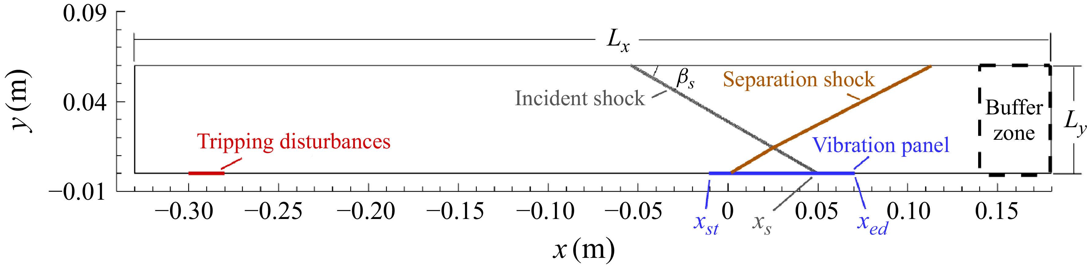

 k=0.41
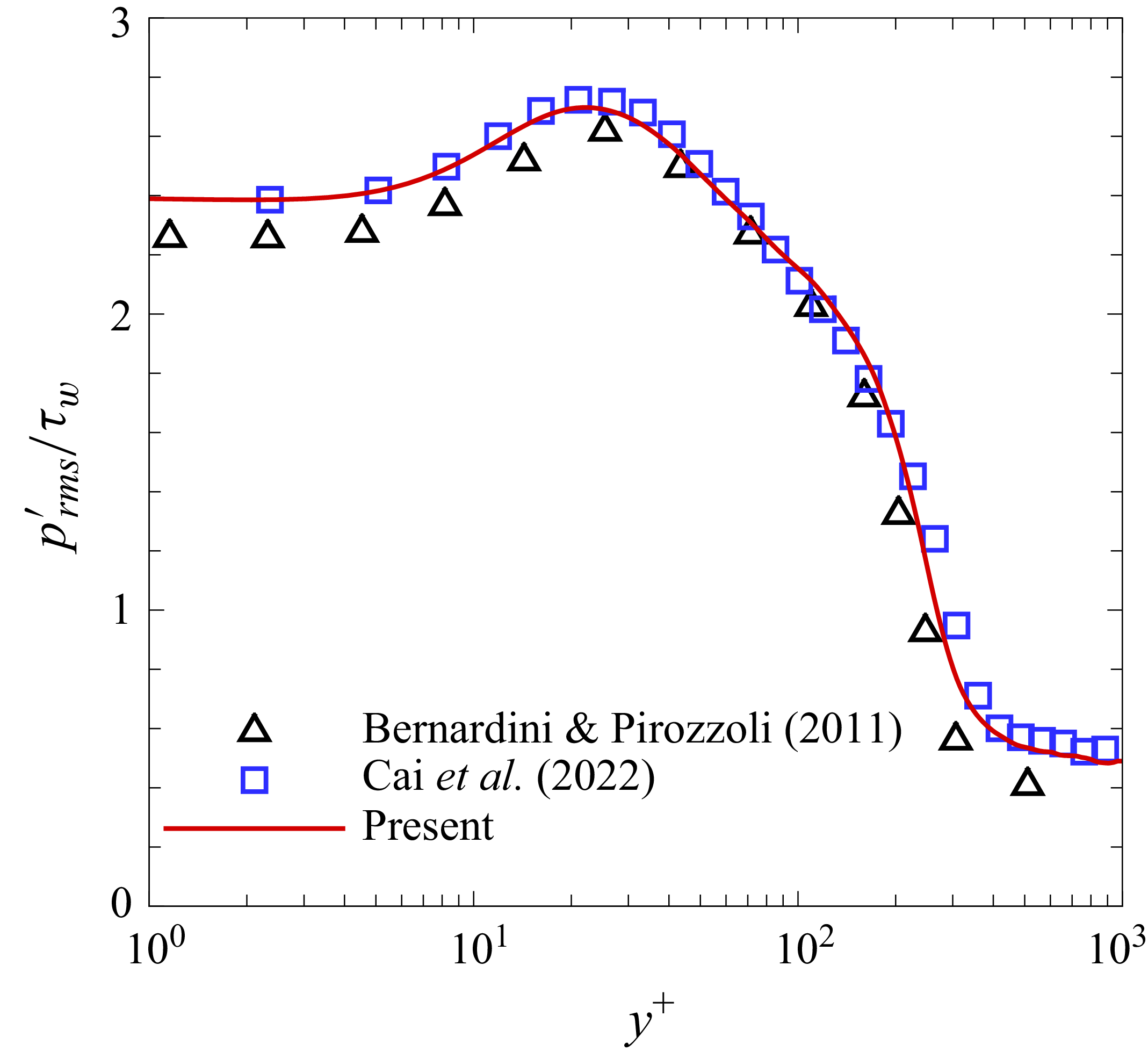
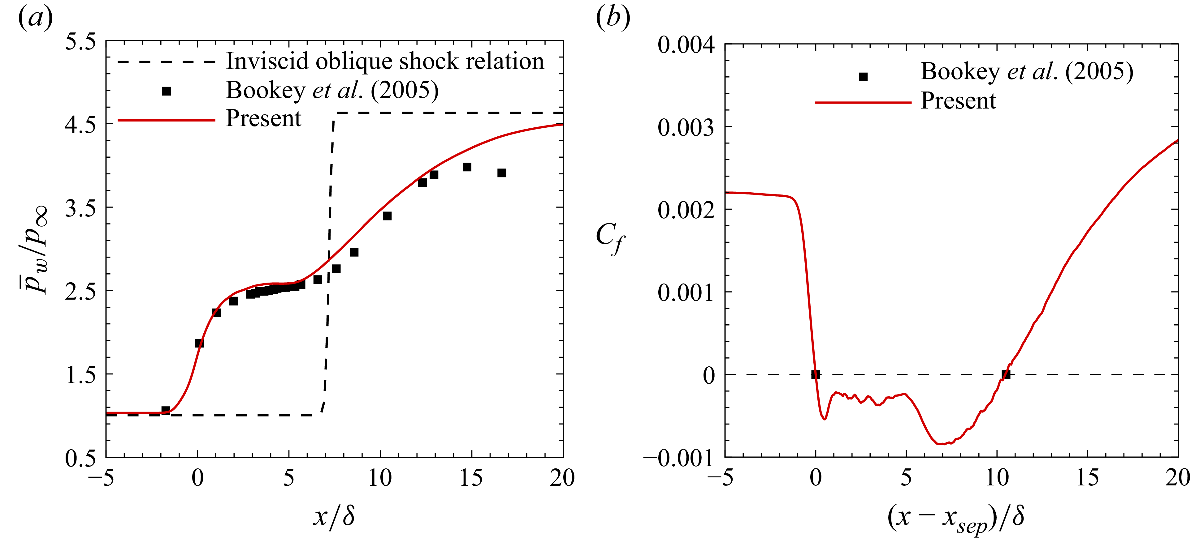


 yw/δ


 π/4
 2π/4
 3π/4
 4π/4
 5π/4
 6π/4
 7π/4
 8π/4

 ΔpPM

 π/4
 2π/4
 3π/4
 4π/4
 5π/4
 6π/4
 7π/4
 8π/4
 uPM=0

 π/4
 2π/4
 3π/4
 4π/4
 5π/4
 6π/4
 7π/4
 8π/4
 uPM=0
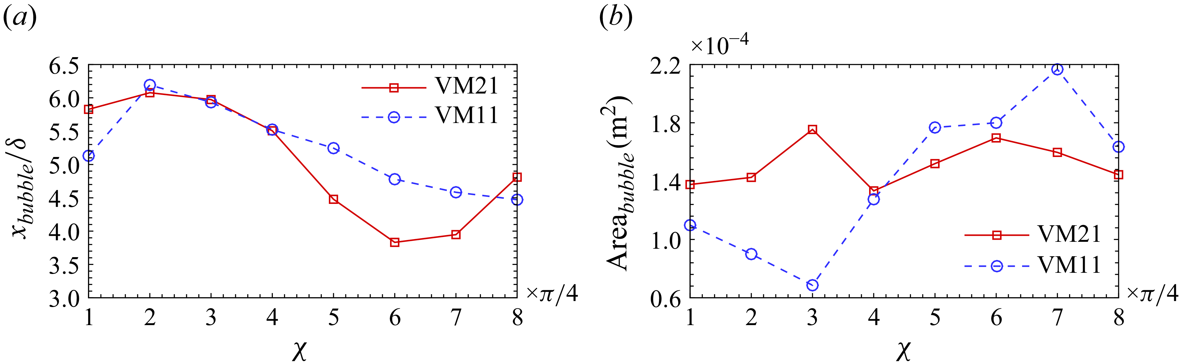

 xref=−3.6δ

 xref=4.0δ

 xref=16.0δ

 u′
 p′

 ϕ1

 ϕ2

 ϕ3

 ϕ1

 ϕ2

 ϕ3


