1 Introduction
Centrifugal forces are ubiquitous in nature and can have a tremendous impact on a large variety of physical systems, ranging from astrophysical objects to man-made experimental devices. Typical examples are accretion disks and planetary cores (Gurnett et al. Reference Gurnett, Persoon, Kurth, Groene, Averkamp, Dougherty and Southwood2007) where centrifugal forces can cause an instability of the system giving rise to spatial patterns strongly affecting its dynamics (Sisan et al. Reference Sisan, Mujica, Tillotson, Huang, Dorland, Hassam, Antonsen and Lathrop2004). At human scale, these centrifugal forces can be found in granular or stratified flows between concentric cylinders (Molemaker, McWilliams & Yavneh Reference Molemaker, McWilliams and Yavneh2001; Conway, Shinbrot & Glasser Reference Conway, Shinbrot and Glasser2004), in separated boundary layer flows (Theofilis, Hein & Dallmann Reference Theofilis, Hein and Dallmann2000; Cherubini et al. Reference Cherubini, Robinet, De Palma and Alizard2010) as well as in a number of confined flows such as the flow within a lid-driven cavity (Ramanan & Homsy Reference Ramanan and Homsy1994; Albensoeder, Kuhlmann & Rath Reference Albensoeder, Kuhlmann and Rath2001; Theofilis et al. Reference Theofilis, Duck and Owen2004). In all cases, if the underlying unstable equilibrium is a two-dimensional flow, centrifugal instabilities trigger a three-dimensionalization of this flow. One of the first striking observations of these three-dimensional centrifugal patterns was reported by Denham & Patrick (Reference Denham and Patrick1974) for the flow over a backward-facing step. This behaviour was later explained by a stability analysis conducted on a spanwise-homogeneous two-dimensional base flow, as reported in Barkley, Gomes & Henderson (Reference Barkley, Gomes and Henderson2002). In such a flow, the primary instability has the form of flat rolls, eventually saturating into counter-rotating elongated vortical structures, the so-called Taylor–Görtler vortices (Beaudoin et al. Reference Beaudoin, Cadot, Aider and Wesfreid2004).
The flow investigated in the present work is the incompressible open cavity flow, also known as the shear-driven cavity flow. It is a geometrically induced separated boundary layer flow having a number of applications in aeronautics. Based on the assumption of two-dimensionality, it has been shown that the leading two-dimensional instability of this flow is mostly localized along the shear layer developing at the interface between the outer boundary layer flow and the inner cavity flow (Sipp et al. Reference Sipp, Marquet, Meliga and Barbagallo2010). This oscillatory global instability of the external shear layer relies on two essential mechanisms: the convectively unstable nature of the shear layer which causes perturbations to grow as they travel downstream, and the instantaneous pressure feedback when the perturbation impacts the downstream corner of the cavity, allowing these same perturbations to eventually re-excite the upstream shear layer and hence giving rise to a linearly unstable feedback loop at sufficiently high Reynolds numbers. For compressible shear-driven cavity flows, a similar unstable feedback loop exists wherein the feedback is given by upstream-propagating acoustic waves (Rossiter Reference Rossiter1964; Rowley, Colonius & Basu Reference Rowley, Colonius and Basu2002; Yamouni, Sipp & Jacquin Reference Yamouni, Sipp and Jacquin2013). This strictly two-dimensional linearly unstable flow configuration has served multiple purposes over the past decade: illustration of optimal control and reduced-order modelling (Barbagallo, Sipp & Schmid Reference Barbagallo, Sipp and Schmid2009), investigation of the nonlinear saturation process of globally unstable flows (Sipp & Lebedev Reference Sipp and Lebedev2007) and introduction to dynamic modes decomposition (Schmid Reference Schmid2010) to name just a few.
Considering strictly two-dimensional perturbations on top of this already two-dimensional base flow is however quite often an over-idealization of the problem. In order to circumvent this drawback, the perturbations are now considered as being spanwise periodic. This ansatz has proved necessary in order to capture the centrifugal instability experienced by the flow. Since the early work of Ramanan & Homsy (Reference Ramanan and Homsy1994) on the stability of a two-dimensional lid-driven cavity toward spanwise-periodic perturbations, a large body of literature has been published wherein this ansatz enables the description of physical instabilities and mechanisms in qualitative agreement with necessarily three-dimensional experimental set-ups. For the lid-driven cavity flow, one can cite Ding & Kawahara (Reference Ding and Kawahara1998), Albensoeder et al. (Reference Albensoeder, Kuhlmann and Rath2001), Guermond et al. (Reference Guermond, Migeon, Pineau and Quartapelle2002), Theofilis et al. (Reference Theofilis, Duck and Owen2004), Albensoeder & Kuhlmann (Reference Albensoeder and Kuhlmann2006), Non, Pierre & Gervais (Reference Non, Pierre and Gervais2006), Chicheportiche et al. (Reference Chicheportiche, Merle, Gloerfelt and Robinet2008), while the reader is referred to the recent works of Meseguer-Garrido et al. (Reference Meseguer-Garrido, de Vicente, Valero and Theofilis2014) and Citro et al. (Reference Citro, Giannetti, Brandt and P.2015a ) and references therein for the shear-driven cavity flow.
Despite its qualitative success, linear stability analysis of a strictly two-dimensional base flow toward spanwise-periodic perturbations is still a relatively restrictive hypothesis, real flows being rarely homogeneous in the spanwise direction. More often than not, flows studied experimentally necessarily have spanwise end walls whose influence cannot be accounted for with the previously cited approach. The existence of such spanwise end walls moreover gives rise to the formation of lateral boundary layers which can induce large-scale secondary motions, which in turn can influence the stability of the flow as demonstrated experimentally by Faure et al. (Reference Faure, Adrianos, Lusseyran and Pastur2007, Reference Faure, Pastur, Lusseyran, Fraigneau and Bish2009) and Douay, Pastur & Lusseyran (Reference Douay, Pastur and Lusseyran2016b ). In order to take properly into account the influence of the spanwise end walls on the stability of the flow, these need to be included in the analysis. The linear stability analysis of a three-dimensional base flow toward three-dimensional perturbations is thus mandatory to obtain a realistic picture. Such fully three-dimensional stability analysis, however, is still a formidable computational task and very few references exist in the literature at this time. One can cite the original work of Bagheri et al. (Reference Bagheri, Schlatter, Schmid and Henningson2009b ), Ilak et al. (Reference Ilak, Schlatter, Bagheri and Henningson2012) and Peplinski, Schlatter & Henningson (Reference Peplinski, Schlatter and Henningson2015) on jets in cross-flow, or Loiseau et al. (Reference Loiseau, Robinet, Cherubini and Leriche2014) and Citro et al. (Reference Citro, Giannetti, Luchini and Auteri2015b ) on roughness-induced transition in boundary layer flows. Feldman & Gelfgat (Reference Feldman and Gelfgat2010), Gómez, Gómez & Theofilis (Reference Gómez, Gómez and Theofilis2014), Kuhlmann & Albensoeder (Reference Kuhlmann and Albensoeder2014) and Loiseau, Robinet & Leriche (Reference Loiseau, Robinet and Leriche2016) have also studied the three-dimensional linear stability of lid-driven cavity flows. To our knowledge, however, the body of literature existing on the instability and transition of realistic three-dimensional shear-driven cavities is essentially limited to Liu, Gómez & Theofilis (Reference Liu, Gómez and Theofilis2016). These authors have reported a linear stability analysis of the flow over a long rectangular open cavity with a narrow span. Their key finding is that, for such long and narrow cavities, the transition to unsteadiness results from an instability of the shear layer reminiscent of the two-dimensional Rossiter modes.
Joining experimental observations, direct numerical simulations and fully three-dimensional linear stability analyses, the present work aims at shedding more light onto the initial stages of transition to unsteadiness of a realistic three-dimensional shear-driven cavity flow. Contrary to Liu et al. (Reference Liu, Gómez and Theofilis2016), we consider herein a relatively large cavity whose aspect ratios are given by
 $L\,:\,D\,:\,S=1\,:\,1\,:\,6$
, where
 $L$
,
 $D$
and
 $S$
are the streamwise length, the depth and the span of the cavity, respectively. Among other things, the results presented herein illustrate the importance of lateral walls to the stability of the flow. They particularly highlight how the spanwise drift of the Taylor–Görtler vortices, reported in a number of experimental studies (Faure et al.
Reference Faure, Pastur, Lusseyran, Fraigneau and Bish2009; Douay et al.
Reference Douay, Pastur and Lusseyran2016b
), is triggered by a secondary instability of the flow which cannot be captured using a traditional two-dimensional assumption of the base flow field. The extremely good agreement between the experimental observations and the predictions of linear stability analyses enables us to provide a simple scenario of the transition to unsteadiness experienced by the flow. The agreement between experimental evidence and theoretical predictions, moreover, strongly supports our claim that the initial stages of transition of the three-dimensional shear-driven cavity flow are solely governed by modal instabilities. The present manuscript is organized as follows. The experimental set-up is presented in § 2 while § 3 describes the numerical set-up and methods used. The fully three-dimensional linear stability analyses performed are presented in § 4. A thorough comparison of the numerical predictions and the experimental observations is given in § 5.1. Finally, § 6 presents our conclusions and some perspectives on this work.
2 Experimental set-up
Experiments reported in the present work were performed in the wind tunnel facility at LIMSI-Orsay (Faure et al.
Reference Faure, Pastur, Lusseyran, Fraigneau and Bish2009; Basley et al.
Reference Basley, Pastur, Delprat and Lusseyran2013, Reference Basley, Pastur, Lusseyran, Soria and Delprat2014; Douay et al.
Reference Douay, Pastur and Lusseyran2016b
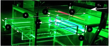
). The experimental set-up is shown in figure 1. The flow is made laminar by a calming section located downstream of the centrifugal fan: it is made of a settling chamber followed by a convergent and two honeycomb panels at the inlet of the contraction duct. The outlet of the wind tunnel is open to the room. The origin of the boundary layer is fixed by an elliptical leading edge, 300 mm upstream of the cavity leading edge, where a Blasius-like velocity profile develops. Background turbulence, estimated by laser Doppler velocimetry, is smaller than 1 %. The wind tunnel force frequencies were mainly distributed between
 $0$
and 10 Hz, with a maximal power around 1 Hz, three orders of magnitude smaller than the cavity flow spectrum for the same frequency range. The span of the wind tunnel is
 $S=300~\text{mm}$
, while the top-to-bottom distance is 75 mm. The cavity depth is
 $D=50~\text{mm}$
. Centrifugal instabilities develop at very low incoming velocity, typically less than
 $1~\text{m}~\text{s}^{-1}$
, which is challenging for the flow rate regulation. The incoming velocity stability is approximately
 $0.025~\text{m}~\text{s}^{-1}$
, which also provides the lower limit of the velocity step. Complete optical access is made available using coated glass walls for the test section and the cavity. The cavity itself consists of three distinct rectangular elements, in coated glass. The first element is a forward-facing step at the inlet of the test section, much deeper than the cavity depth. The second element is the base floor which sets the cavity depth
 $D$
. Finally, the last element is a
 $D$
-deep forward-facing step which can slide above the flat floor of the second element, so as to adjust the cavity length
 $L$
. As the flow is sensitive to inaccuracies in the cavity assembly, we had to pay particular attention to suppress any leak that could be present at the edges and corners of the cavity. In addition, the incoming flow has a very small, though non-vanishing, spanwise component, introducing a systematic bias in the incoming flow direction which is not strictly streamwise. Visualizations of the flow patterns presented later on are carried out by lighting up the smoke produced by a fog machine with a laser sheet generated by a 200 mJ Quantel twin-pulsed YAG laser. A standard, single-frame video camera (AVT Cameras, Marlin,
 $1024~\text{pixel}\times 768~\text{pixel}$
of size
 $4.65~\unicode[STIX]{x03BC}\text{m}\times 4.65~\unicode[STIX]{x03BC}\text{m}$
with resolution depth of 8 bit) snaps images at a frame rate of 20 Hz. An electronic delay generator (R&D Vision) is used to synchronize flash lamps and Q-switches of both laser cavities together with the camera’s through the lens (TTL) signal.
Picture of the experimental set-up at LIMSI (Orsay, France), as described by Faure et al. (Reference Faure, Adrianos, Lusseyran and Pastur2007).

3 Problem statement and numerical methods
3.1 Governing equations
The dynamics of the incompressible flow of a Newtonian fluid over an open cavity is governed by the Navier–Stokes equations
 $$\begin{eqnarray}\displaystyle & \displaystyle \frac{\unicode[STIX]{x2202}\boldsymbol{u}}{\unicode[STIX]{x2202}t}=-(\boldsymbol{u}\boldsymbol{\cdot }\unicode[STIX]{x1D735})\boldsymbol{u}-\unicode[STIX]{x1D735}p+\frac{1}{Re}\unicode[STIX]{x1D6FB}^{2}\boldsymbol{u}, & \displaystyle\end{eqnarray}$$
 $$\begin{eqnarray}\displaystyle & \displaystyle \unicode[STIX]{x1D735}\boldsymbol{\cdot }\boldsymbol{u}=0, & \displaystyle\end{eqnarray}$$
where
 $\boldsymbol{u}=(u(\boldsymbol{x},t),v(\boldsymbol{x},t),w(\boldsymbol{x},t))^{\text{T}}$
is the velocity field and
 $p(\boldsymbol{x},t)$
is the pressure field. The Reynolds number is defined as
 $Re=U_{\infty }L/\unicode[STIX]{x1D708}$
, where
 $U_{\infty }$
is the free-stream velocity,
 $L$
is the length of the cavity and
 $\unicode[STIX]{x1D708}$
is the kinematic viscosity of the fluid. The reference frame
 $\boldsymbol{x}=(x,y,z)^{\text{T}}$
is chosen such that
 $x$
is the streamwise,
 $y$
the wall-normal and
 $z$
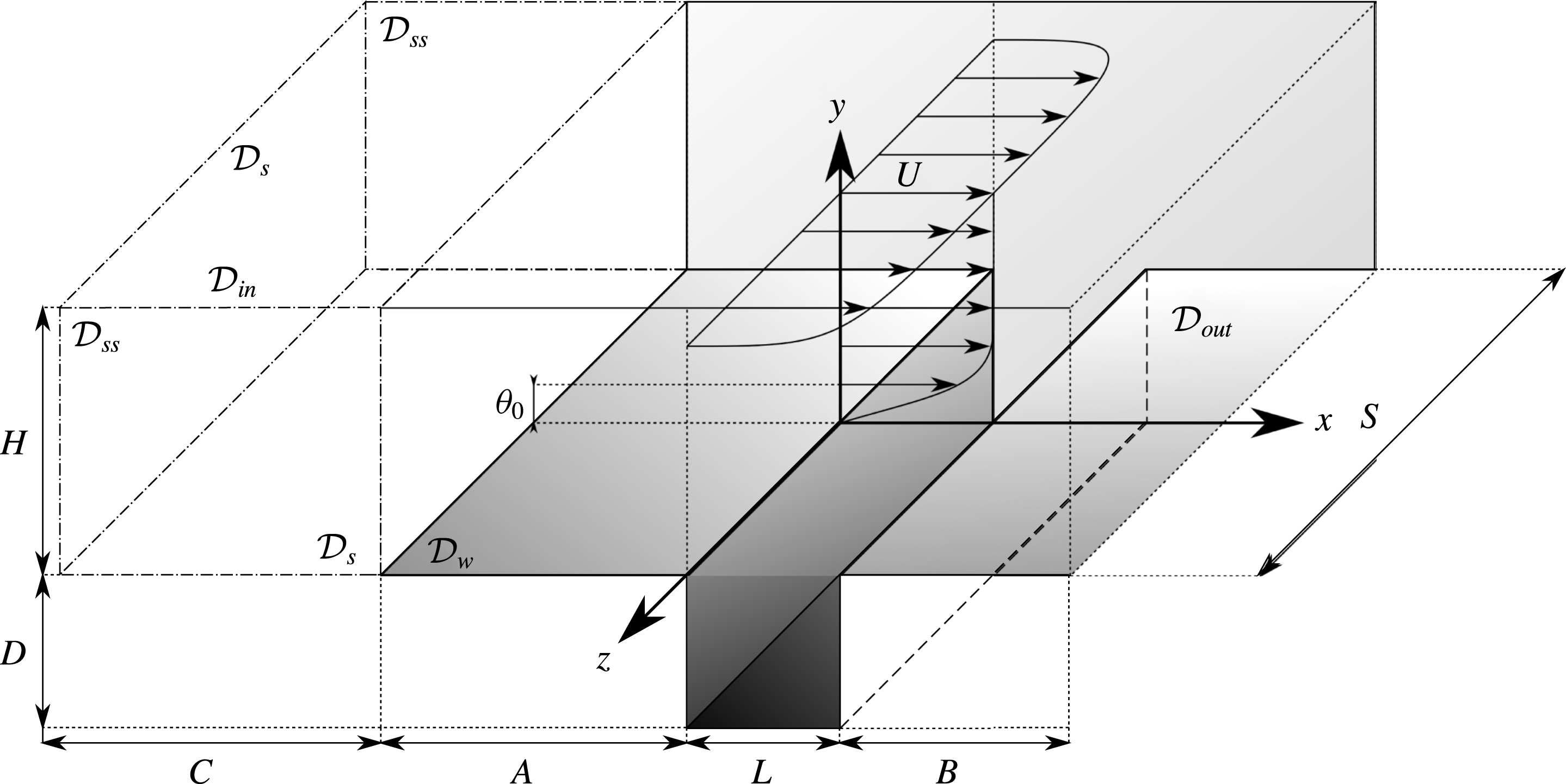
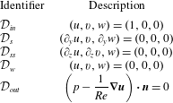
the spanwise direction. The flow configuration is sketched in figure 2, where the boundary conditions are indicated using the symbols listed in table 1. Following Sipp & Lebedev (Reference Sipp and Lebedev2007) and Citro et al. (Reference Citro, Giannetti, Brandt and P.2015a
), a fully three-dimensional boundary layer is obtained from a free-slip/no-slip discontinuity in the boundary condition.
Sketch of a three-dimensional open cavity flow, showing the geometrical features. The shaded areas highlight the walls where no-slip boundary conditions are imposed.

The Navier–Stokes equations are solved using the incompressible flow solver Nek5000 (Fischer et al.
Reference Fischer, Kruse, Mullen, Tufo, Lottes and Kerkemeier2008) which is based on the spectral element method (SEM). A
 $\mathbb{P}_{N}-\mathbb{P}_{N-2}$
formulation has been used: the velocity field is discretized using
 $N$
th degree Lagrange interpolants, defined on the Gauss–Legendre–Lobatto quadrature points, as basis and trial functions, while the pressure field is discretized using Lagrange interpolants of degree
 $N-2$
defined on the Gauss–Legendre quadrature points. Finally, the time integration is performed using the BDF3/EXT3 scheme: integration of the viscous terms relies on the backward differentiation (BDF3), while the convective terms are integrated via extrapolation (EXT3), both methods being third-order accurate. The Navier–Stokes equations are discretized on a mesh of 30 000 spectral elements with polynomials of order 8. Thus, the problem to be solved consists of over
 $61$
million degrees of freedom for describing the velocity and pressure fields.
Description of the boundary conditions, with reference to figure 2.

3.2 Linear stability analysis
Steady solutions
 $\boldsymbol{Q}(\boldsymbol{x})=(\boldsymbol{U}_{b},P_{b})^{\text{T}}$
to the Navier–Stokes equations are known as base flows or fixed points of the system. Their linear stability is dictated by the fate of infinitesimal perturbations evolving in their vicinity. The dynamics of such perturbations is governed by the linearized Navier–Stokes equations, which can be compactly written as
 $$\begin{eqnarray}\frac{\unicode[STIX]{x2202}\boldsymbol{u}}{\unicode[STIX]{x2202}t}=\boldsymbol{J}\boldsymbol{u}\end{eqnarray}$$
once projected onto a divergence-free vector space. As this linear dynamical system is autonomous in time, the perturbation
 $\boldsymbol{u}$
can be expanded into normal modes, such that
 $\boldsymbol{u}(\boldsymbol{x},t)=\sum _{k=1}^{\infty }\hat{\boldsymbol{u}}_{k}(\boldsymbol{x})\exp (\unicode[STIX]{x1D706}_{k}t)$
. Injecting this normal mode ansatz into (3.3) yields an eigenvalue problem
 $$\begin{eqnarray}\unicode[STIX]{x1D706}\hat{\boldsymbol{u}}=\boldsymbol{J}\hat{\boldsymbol{u}},\end{eqnarray}$$
where
 $\unicode[STIX]{x1D706}=\unicode[STIX]{x1D70E}+\text{i}\unicode[STIX]{x1D714}$
is the eigenvalue and
 $\hat{\boldsymbol{u}}$
its associated eigenvector. The linear stability of the fixed point is then dictated by the real part
 $\unicode[STIX]{x1D70E}$
of the most unstable/least stable eigenvalue: the base flow is linearly unstable if
 $\unicode[STIX]{x1D70E}>0$
, otherwise it is linearly stable. Boundary conditions used to solve (3.4) are the same as those given in table 1, except at the inflow where a zero-velocity Dirichlet condition is now prescribed. It has to be noted however that because of the large number of degrees of freedom, solving the eigenproblem (3.3) using direct methods (i.e. QR or QZ algorithms) is hardly possible at the moment. Following Edwards et al. (Reference Edwards, Tuckerman, Friesner and Sorensen1994) and Bagheri et al. (Reference Bagheri, Åkervik, Brandt and Henningson2009a
), a time-stepper formulation of the problem is thus used. The leading eigenpairs of the linearized Navier–Stokes operator are then obtained based on the iterative Arnoldi algorithm (Arnoldi Reference Arnoldi1951) described by Loiseau et al. (Reference Loiseau, Robinet, Cherubini and Leriche2014) using a Krylov subspace of dimension
 $K=250$
and a sampling period
 $\unicode[STIX]{x0394}T=2.5$
in non-dimensional time units. For this selected set of parameters, each stability computation employs a wall-clock time of 15 to 20 h on 512–1024 cores. Thus, up to
 $20\,000$
CPU hours are needed to obtain one eigenvalue spectrum (without considering the CPU time for computing the base flow by continuation).
4 Results
4.1 Primary bifurcation
4.1.1 Base flow
As will be shown, the first bifurcation experienced by the flow results from an eigenvalue of the linearized Navier–Stokes operator crossing the neutral growth rate axis, which is characterized by a zero frequency. The corresponding eigenmode thus experiences an exponential growth but does not exhibit periodic oscillation. Consequently, the popular selective frequency damping (Åkervik et al. Reference Åkervik, Brandt, Henningson, Hoepffner, Marxen and Schlatter2006) cannot quench its development, and a continuation method similar to Theofilis & Colonius (Reference Theofilis and Colonius2003) is thus used to compute linearly unstable base flows close to the first bifurcation threshold.
(a) Colour map of the velocity magnitude of the base flow at
 $Re=3300$
in the symmetry
 $z=0$
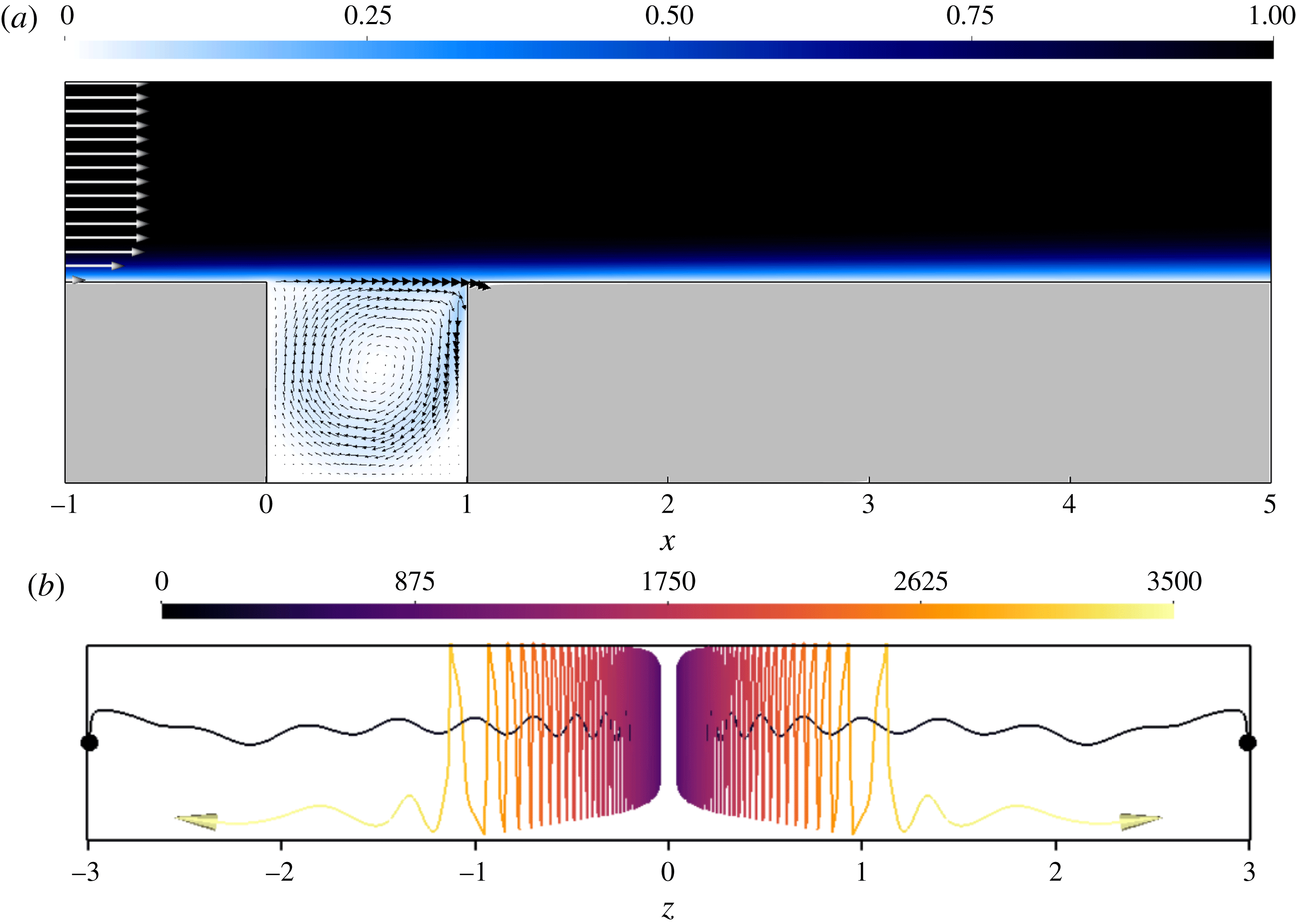
vertical plane. Only a subset of the whole computational domain is considered. (b) Visualization of the path lines of two particles located initially at
 $(x,y,z)=(0.5,-0.5,\pm 2.99)$
. The incoming flow is directed toward the reader. The colour scale indicates the trajectory integration time.

Figure 3 depicts some of the key features of the primary base flow. Though it is fully three-dimensional due to the spanwise end walls being taken into consideration, it can be seen that the flow within the central plane (given by
 $z=0$
) looks quite similar to its two-dimensional counterpart: see figure 3(a). Despite this apparent resemblance, the three-dimensionality of the flow within the cavity is clearly visible in figure 3(b) depicting some of the streamlines of the inner cavity flow. Fluid particles in the vicinity of the spanwise end walls are attracted toward the
 $z=0$
plane along the central vortex. This spanwise flow results from the interaction between the swirling flow within the central plane and the zero-velocity condition prescribed at the spanwise end walls. Because of the friction along these end walls, the
 $x$
- and
 $y$
-velocity components are damped. However, due to the incompressibility of the flow, this deceleration of the
 $(x,y)$
in-plane motion gives rise to a secondary flow which is directed along the
 $z$
-axis as illustrated by the streamline visualizations. This secondary flow, from the spanwise end walls toward the central plane of the cavity, occurs within the core of the primary vortex which experiences a solid-body-like rotation. Once it has reached the central plane, the fluid particles stay in its vicinity for a while before being expelled toward the end walls.
(a) Eigenspectra of the linearized Navier–Stokes operator for
 $Re=3400$
(blue squares) and
 $Re=3475$
(red circles). The shaded region corresponds to the stable part of the complex plane. (b) Spanwise velocity isocontours of the leading unstable mode at
 $Re=3475$
. (c) Motion induced by this mode in the
 $y=-0.5$
horizontal plane. The colour map depicts the amplitude of the out-of-plane (vertical) velocity component while the vectors show the in-plane motion.

4.1.2 Eigenspectra and eigenfunctions
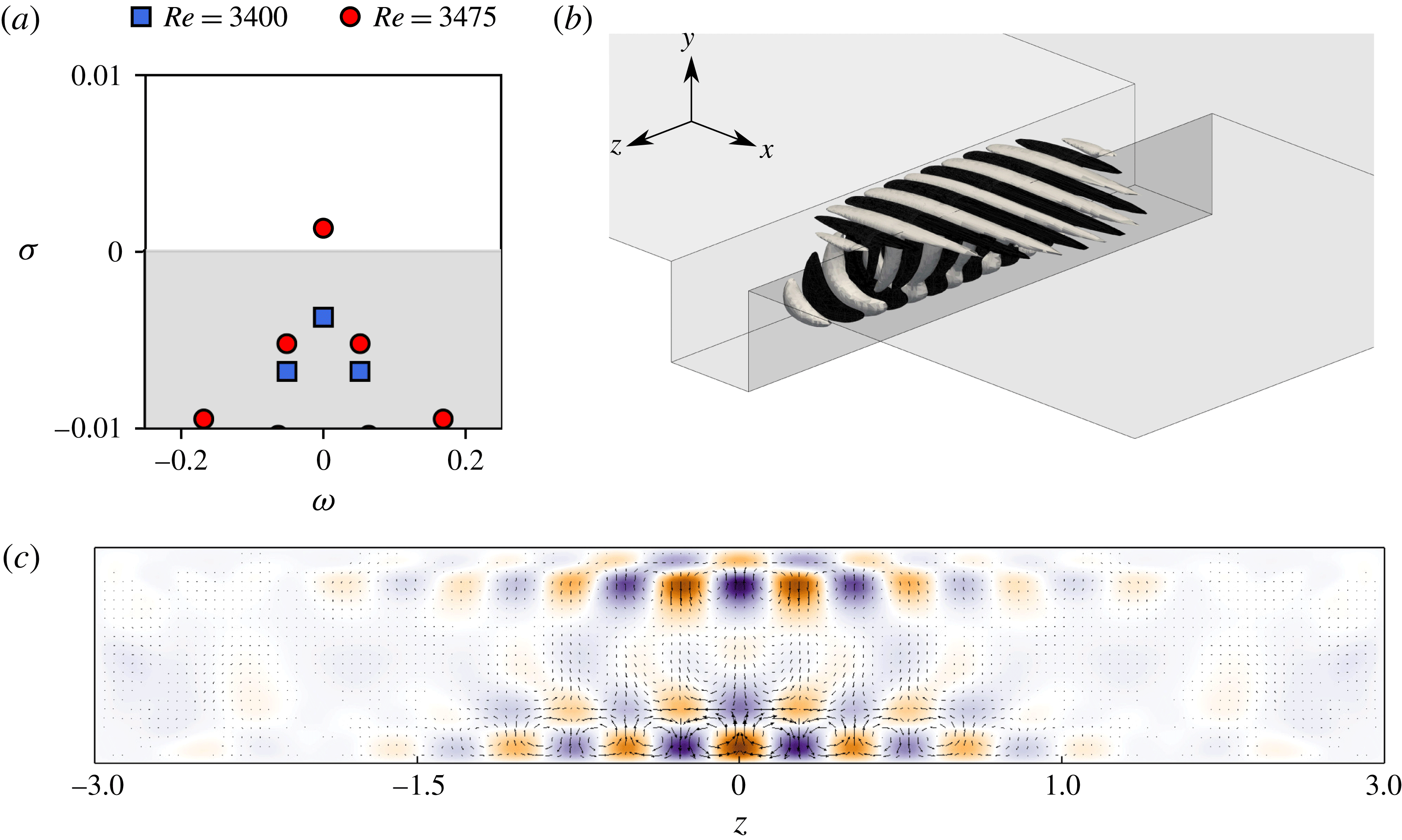
Figure 4(a) depicts the eigenspectra of the linearized Navier–Stokes operator at
 $Re=3400$
and
 $Re=3475$
. All the eigenmodes are stable at
 $Re=3400$
(blue squares). Increasing the Reynolds number, a real eigenvalue crosses the neutral axis becoming unstable (red dots). A linear interpolation gives a critical Reynolds number
 $Re_{C1}=3450$
. Spanwise velocity contours of the eigenvector corresponding to the leading eigenvalue are depicted in figure 4(b), while the motion induced in the
 $y=-0.5$
horizontal plane is highlighted in figure 4(c). It consists of a set of counter-rotating Taylor–Görtler-like vortices. Similar unstable structures also appear in the canonical lid-driven cavity flow (Albensoeder et al.
Reference Albensoeder, Kuhlmann and Rath2001; Ramanan & Homsy Reference Ramanan and Homsy1994; Non et al.
Reference Non, Pierre and Gervais2006; Chicheportiche et al.
Reference Chicheportiche, Merle, Gloerfelt and Robinet2008; Theofilis et al.
Reference Theofilis, Duck and Owen2004; Feldman & Gelfgat Reference Feldman and Gelfgat2010; Loiseau et al.
Reference Loiseau, Robinet and Leriche2016). Similar modes for the two-dimensional shear-driven cavity flow have been computed by Bres & Colonius (Reference Bres and Colonius2008), Meseguer-Garrido et al. (Reference Meseguer-Garrido, de Vicente, Valero and Theofilis2014), de Vicente et al. (Reference de Vicente, Basley, Meseguer-Garrido, Soria and Theofilis2014) and observed experimentally by Faure et al. (Reference Faure, Adrianos, Lusseyran and Pastur2007, Reference Faure, Pastur, Lusseyran, Fraigneau and Bish2009), Douay et al. (Reference Douay, Pastur and Lusseyran2016b
) and Douay, Lusseyran & Pastur (Reference Douay, Lusseyran and Pastur2016a
). A Fourier decomposition of the mode in the spanwise direction indicates that the dominant wavelength is
 $\unicode[STIX]{x1D706}_{z}=0.515$
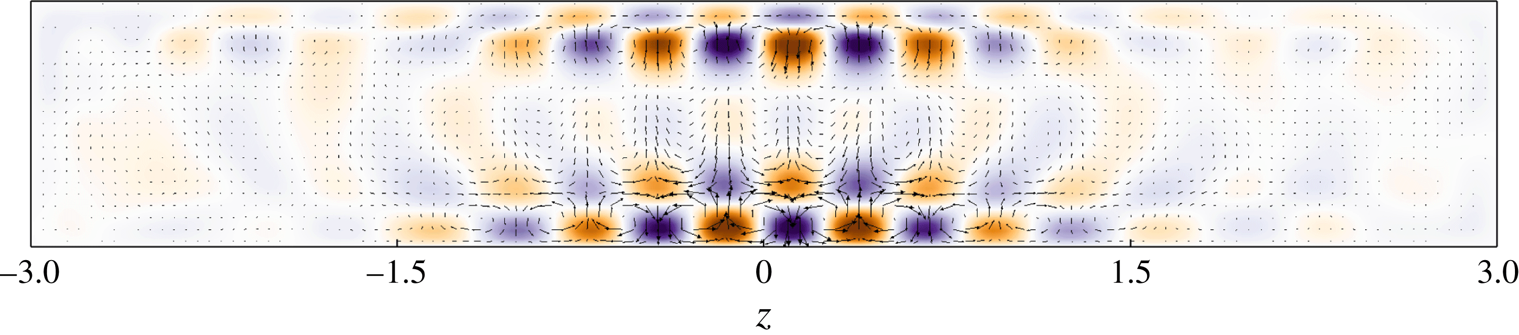
, in good agreement with previous findings. Finally, it has to be noted that, on the eigenspectra depicted in figure 4(a), a second real eigenvalue is almost indiscernible from the leading unstable one, their growth rates differing by less than 1 %. The spatial distribution of the eigenvector associated with this eigenvalue is shown in figure 5. Comparing figures 4(c) and 5, these two eigenfunctions appear to be quite similar, both exhibiting the same spanwise wavenumber
 $\unicode[STIX]{x1D706}_{z}\simeq 0.51$
. However, while the eigenfunction associated with the most unstable eigenvalue exhibits a mirror symmetry, the one associated with the least unstable eigenvalue displays a mirror antisymmetry. Although this antisymmetric eigenmode is linearly unstable at the Reynolds numbers considered, it has never been observed in our direct numerical simulations. A similar observation has also been reported by Loiseau (Reference Loiseau2014) for three-dimensional lid-driven cavity flows. From a mathematical point of view, both of these two modes can be traced back to the same leading spanwise-periodic instability mode
 $\hat{\boldsymbol{u}}(x,y,\unicode[STIX]{x1D6FD})$
of the two-dimensional shear-driven cavity. The mirror-symmetric mode would then asymptotically tend to
 $$\begin{eqnarray}\lim _{S\rightarrow \infty }\boldsymbol{u}(x,y,z)=\hat{\boldsymbol{u}}(x,y)\cos (\unicode[STIX]{x1D6FD}z),\end{eqnarray}$$
where
 $S$
is the spanwise extent of the cavity, while the mirror-antisymmetric mode would tend to
 $$\begin{eqnarray}\lim _{S\rightarrow \infty }\boldsymbol{u}(x,y,z)=\hat{\boldsymbol{u}}(x,y)\sin (\unicode[STIX]{x1D6FD}z).\end{eqnarray}$$
It is unclear at the present time whether these two eigenvalues are non-degenerate eigenvalues or if they are the same degenerate eigenvalue with a multiplicity 2.
Motion induced by the least unstable mode in the
 $y=-0.5$
horizontal plane at
 $Re=3475$
. The colour map depicts the amplitude of the out-of-plane (vertical) velocity component while the vectors show the in-plane motion. Note that, contrary to the unstable mode, this one is characterized by a mirror antisymmetry.

4.1.3 Physical mechanism
Following Albensoeder et al. (Reference Albensoeder, Kuhlmann and Rath2001), the velocity field
 $\boldsymbol{u}$
of the leading eigenvector is decomposed as
 $$\begin{eqnarray}\boldsymbol{u}=\boldsymbol{u}_{\Vert }+\boldsymbol{u}_{\bot },\end{eqnarray}$$
where
 $\boldsymbol{u}_{\Vert }$
is everywhere parallel to the direction of the base flow velocity vectors, while
 $\boldsymbol{u}_{\bot }$
is its orthogonal complement. Using such a decomposition, the unstable eigenmode can be understood as the superposition of two structures: counter-rotating rolls (
 $\boldsymbol{u}_{\bot }$
) and streaky structures (
 $\boldsymbol{u}_{\Vert }$
) aligned with the flow. While the rolls account for 40 % of the perturbation’s kinetic energy, the remaining 60 % is provided by the streaky structure. Introducing this decomposition into the Reynolds–Orr equation governing the evolution of the perturbation’s kinetic energy, the production term
 $P=-\!\int _{V}\boldsymbol{u}\boldsymbol{\cdot }(\boldsymbol{u}\boldsymbol{\cdot }\unicode[STIX]{x1D735})\boldsymbol{U}_{b}\,\text{d}V$
can be decomposed into the following four terms:
 $$\begin{eqnarray}I_{1}=-\int _{V}\boldsymbol{u}_{\bot }\boldsymbol{\cdot }(\boldsymbol{u}_{\bot }\boldsymbol{\cdot }\unicode[STIX]{x1D735})\boldsymbol{U}_{b}\,\text{d}V,\quad I_{2}=-\!\int _{V}\boldsymbol{u}_{\Vert }\boldsymbol{\cdot }(\boldsymbol{u}_{\bot }\boldsymbol{\cdot }\unicode[STIX]{x1D735})\boldsymbol{U}_{b}\,\text{d}V,\end{eqnarray}$$
 $$\begin{eqnarray}I_{3}=-\!\int _{V}\boldsymbol{u}_{\bot }\boldsymbol{\cdot }(\boldsymbol{u}_{\Vert }\boldsymbol{\cdot }\unicode[STIX]{x1D735})\boldsymbol{U}_{b}\,\text{d}V,\quad I_{4}=-\!\int _{V}\boldsymbol{u}_{\Vert }\boldsymbol{\cdot }(\boldsymbol{u}_{\Vert }\boldsymbol{\cdot }\unicode[STIX]{x1D735})\boldsymbol{U}_{b}\,\text{d}V.\end{eqnarray}$$
A different physical mechanism is associated with each of these four contributions. For instance, the
 $I_{2}$
term is associated with the lift-up mechanism (Landahl Reference Landahl1980), consisting of the transport of the base flow shear by counter-rotating rolls
 $\boldsymbol{u}_{\bot }$
, which induce streaky structures
 $\boldsymbol{u}_{\Vert }$
, whereas the
 $I_{3}$
term is linked to the anti-lift-up mechanism, an energy amplification mechanism typically found in stable columnar vortices (Antkowiak & Brancher Reference Antkowiak and Brancher2007). The sign of the different integrals
 $I_{i}$
then indicates whether the associated physical mechanism acts to promote (positive) or quench (negative) the instability considered. The contributions of these different production terms to the total kinetic energy budget are summarized in table 2. This energy budget is dominated by the
 $I_{2}$
term, characterizing the transfer of energy between the base flow and the perturbation through the lift-up mechanism (Landahl Reference Landahl1980). Very similar energy budgets have been obtained for lid-driven cavity flows by Albensoeder et al. (Reference Albensoeder, Kuhlmann and Rath2001) and Loiseau et al. (Reference Loiseau, Robinet and Leriche2016), pointing to an instability of centrifugal type.
Contribution of the different production terms
 $I_{i}$
and the viscous dissipation
 $D$
to the total kinetic energy budget of the unstable mode at
 $Re=3500$
.

4.1.4 Nonlinear evolution
Starting from the linearly unstable base flow at
 $Re=3500$
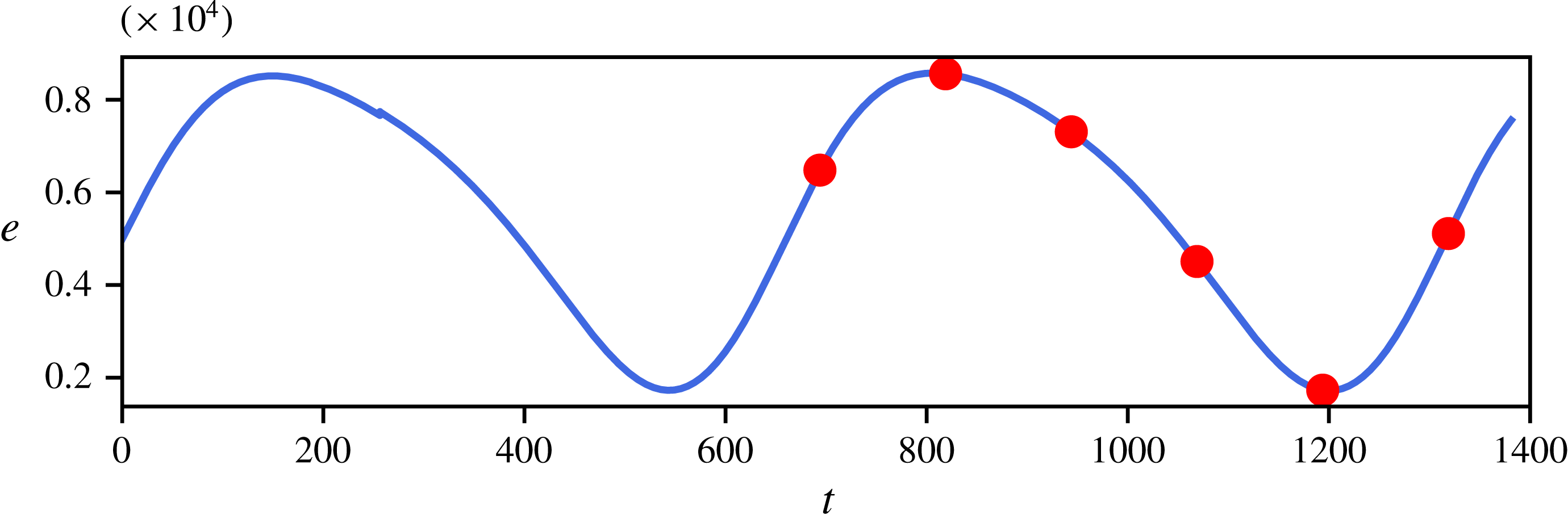
, a direct numerical simulation has been run until nonlinear saturation is reached in order to gain a better understanding of the saturation process of the instability and of the flow it is giving rise to. Figure 6 depicts the evolution of the flow’s kinetic energy once an almost statistical steady state has been reached. Although the linear stability predicts a non-oscillatory instability, a surprising low-frequency (
 $\unicode[STIX]{x1D714}\approx 0.009$
) and low-amplitude (
 $\text{std}\approx 2.5\times 10^{-5}$
) oscillation of the perturbation’s energy can be observed. At the present time, it is not clear how this oscillation arises. Two different hypotheses can be formulated.
(i) The combination of the Krylov subspace’s dimension and of the sampling period of the snapshots does not allow us to span a sufficiently large number of periods of this low-frequency oscillation for the Arnoldi algorithm to appropriately estimate its phase, and hence the imaginary part of the leading eigenvalue.
(ii) Assuming the linear eigenmode is indeed non-oscillatory, the low-frequency low-amplitude oscillation observed might arise from nonlinear interaction between this mode and the secondary low-energy spanwise flow induced by the existence of the spanwise end walls discussed earlier.
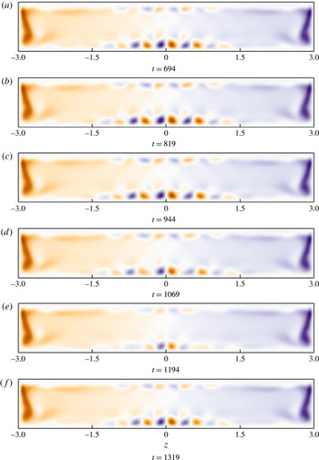
The first hypothesis highlights potential limitations of the time-stepping approach when applied to linear stability analysis. Unfortunately, given our computational resources, it is not currently possible to increase significantly the dimension of the Krylov subspace and the associated sampling period in order to span several periods of this low-frequency oscillation. On the other hand, verifying the second hypothesis would rely on weakly nonlinear analyses (Sipp & Lebedev Reference Sipp and Lebedev2007) which are still very challenging for fully three-dimensional flow configurations and are beyond the scope of the present work. Figure 7 depicts the instantaneous spatial distribution of the helicity
 $\boldsymbol{h}(\boldsymbol{x},t)=\boldsymbol{u}(\boldsymbol{x},t)\boldsymbol{\cdot }\unicode[STIX]{x1D74E}(\boldsymbol{x},t)$
within the
 $y=-0.5$
horizontal plane at six different instants of time. As shown, the linearly unstable eigenmode reported in the previous section gives rise to five pairs of Taylor–Görtler-like vortices, the three central ones being largely more energetic than the outermost ones. These helicity maps also underline the strong swirling motion experienced by the fluid particles in the vicinity of the lateral walls and already outlined previously for the primary base flows: see figure 3(b). Looking at these different snapshots, it can finally be observed that the low-frequency oscillation observed in the flow’s kinetic energy evolution depicted on figure 6 spatially corresponds to a small spanwise oscillation of these Taylor–Görtler-like vortices. Although a small change in the amplitude of the helicity is noticeable, one needs to recall that it occurs over several hundreds of convective time units. Moreover, it can be seen that these Taylor–Görtler vortices remain within the central part of the cavity delimited by
 $-1.5\leqslant z\leqslant 1.5$
.
Evolution of the perturbation’s kinetic energy as a function of time in the nonlinearly saturated regime at
 $Re=3500$
. Note that the vertical axis has been re-scaled by a factor
 $10^{4}$
. The red dots indicate the instants of time for which the corresponding helicity fields are depicted in figure 7.

Snapshots of the instantaneous helicity field
 $\boldsymbol{h}(\boldsymbol{x},t)=\unicode[STIX]{x1D74E}(\boldsymbol{x},t)\boldsymbol{\cdot }\boldsymbol{u}(\boldsymbol{x},t)$
at the different instants of time highlighted in figure 6 (
 $Re=3500$
). The colour scale has been kept constant over the different figures.

4.2 Secondary bifurcation
4.2.1 Base flow
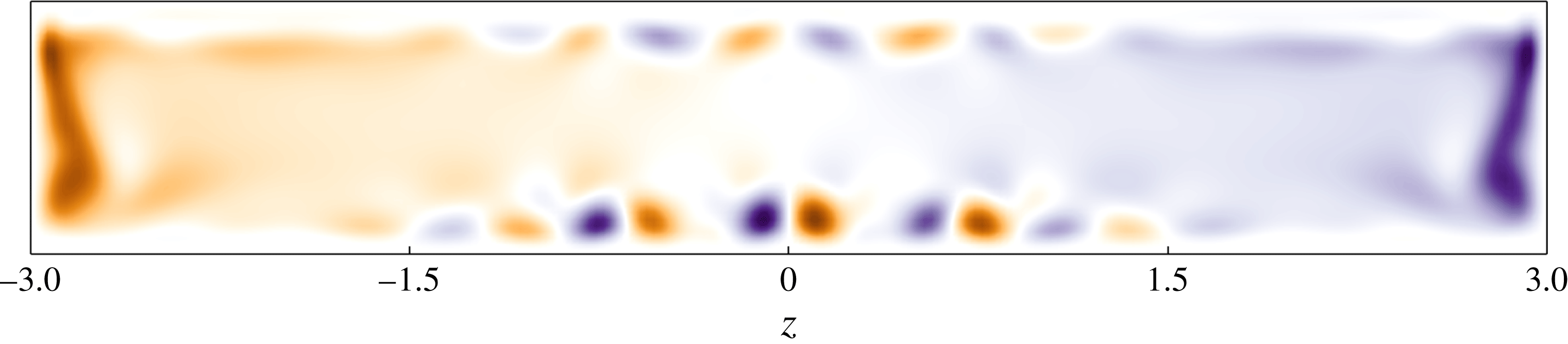
As shown in the previous section, the primary bifurcation gives rise to a flow characterized by a very low-frequency and low-amplitude oscillation of the central Taylor–Görtler-like vortices. Figure 8 depicts the instantaneous spatial distribution of the helicity
 $\boldsymbol{h}(\boldsymbol{x})$
within the
 $y=-0.5$
horizontal plane at
 $Re=3700$
. It can be seen that the structure of the bifurcated flow is hardly modified when increasing the Reynolds number. A similar observation can be made regarding the frequency of the low-amplitude oscillation of the flow’s kinetic energy (not shown). From a quantitative point of view, the total rate of change of the velocity field over
 $\unicode[STIX]{x0394}t=2.5\times 10^{-3}$
non-dimensional time units is of the order of
 $10^{-6}$
–
 $10^{-7}$
. For linear stability analysis purposes, such a slowly evolving flow can thus be considered as being quasi-stationary and be used as a base flow. Since this small unsteadiness is moreover limited to the region
 $-1.5\leqslant z\leqslant 1.5$
, this quasi-static assumption is further strengthened a posteriori given that the spatial support of the second linearly unstable mode is almost entirely localized within the
 $\Vert z\Vert \geqslant 1.5$
region, as will be shown in the next section.
Helicity field of the bifurcated base flow within the
 $y=-0.5$
horizontal plane. The Reynolds number is set to
 $Re=3700$
.

4.2.2 Eigenspectra and eigenfunctions
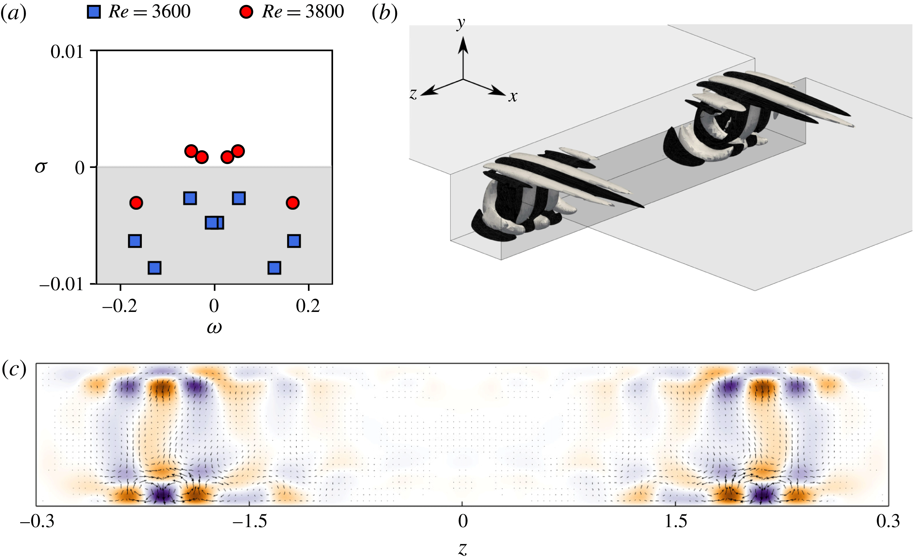
Figure 9(a) depicts the eigenspectra of the linearized Navier–Stokes operator at
 $Re=3600$
and
 $Re=3800$
. While for
 $Re=3600$
all the modes are stable, it can be seen that at
 $Re=3800$
two complex conjugate pairs of eigenvalues lie in the upper-half complex plane:
 $\unicode[STIX]{x1D706}_{2}=0.0013\pm \text{i}0.0496$
and
 $\unicode[STIX]{x1D706}_{3}=0.0008\pm \text{i}0.0272$
, respectively. A linear interpolation gives a critical Reynolds number
 $Re_{C2}=3730$
for the eigenvalue
 $\unicode[STIX]{x1D706}_{2}$
. The second bifurcation of the flow hence results from a pair of complex conjugate eigenvalues moving into the upper-half complex plane, i.e. an Andronov–Poincaré–Hopf bifurcation. Consequently, it leads the flow to exhibit self-sustained oscillations characterized by a circular frequency
 $\unicode[STIX]{x1D714}=\pm 0.0496$
, i.e. four to five times larger than the low frequency of the low-amplitude oscillation of the base flow. The fact that a second unstable mode,
 $\unicode[STIX]{x1D706}_{3}$
, is observed at
 $Re=3800$
indicates the existence of a second Hopf bifurcation, at a critical Reynolds number
 $Re_{C3}=3770$
resulting from the eigenvalue
 $\unicode[STIX]{x1D706}_{3}$
stepping into the upper-half complex plane.
Spanwise velocity contours of the eigenvector corresponding to the leading eigenvalue
 $\unicode[STIX]{x1D706}_{2}$
are depicted in figure 9(b), while the motion induced in the
 $y=-0.5$
horizontal plane is depicted in figure 9(c). Note that the eigenvector associated with
 $\unicode[STIX]{x1D706}_{3}$
is quite similar and is thus not shown for the sake of conciseness. Whereas the spatial support of the unstable eigenmode at the bifurcation point
 $Re_{C1}=3430$
is mostly localized in the central part of the cavity (
 $\Vert z\Vert \leqslant 1.5$
) (see figure 4), that depicted in figure 9 is essentially located in the outer part of the cavity given by
 $\Vert z\Vert \geqslant 1.5$
. Although its spatial support lets us hypothesize that it is related to the existence of the spanwise end walls, it nonetheless takes the form of Taylor–Görtler-like vortices characterized by a spanwise wavelength
 $\unicode[STIX]{x1D706}_{z}=0.49$
. As previously, this unstable eigenmode can be decomposed as
 $\boldsymbol{u}=\boldsymbol{u}_{\Vert }+\boldsymbol{u}_{\bot }$
, with 61 % of the kinetic energy of the mode contained in the streaky structure
 $\boldsymbol{u}_{\Vert }$
while the rolls account for the remaining 39 %. Despite their different spatial locations, both the primary and secondary unstable eigenmodes hence appear to rely on the same underlying physical mechanisms. This is further confirmed by table 3, providing the contribution of the different productions terms
 $I_{i}$
to the total kinetic energy budget. Once again, this energy budget is dominated by the
 $I_{2}$
term, hence implying that this secondary instability is also of centrifugal type. Finally, it is worth noting that the pair of complex conjugate eigenvalues now becoming unstable could already be foreseen at lower Reynolds numbers: see the least stable complex conjugate eigenvalues in the eigenspectrum shown in figure 4(a).
(a) Eigenspectra of the linearized Navier–Stokes operator for
 $Re=3600$
(blue squares) and
 $Re=3800$
(red circles). The shaded region corresponds to the stable part of the complex plane. (b) Spanwise velocity isocontours of the leading unstable mode at
 $Re=3800$
. (c) Motion induced by this mode in the
 $y=-0.5$
horizontal plane. The colour map depicts the amplitude of the out-of-plane (vertical) velocity component while the vectors show the in-plane motion.

Contribution of the different production terms
 $I_{i}$
and the viscous dissipation
 $D$
to the total kinetic energy budget of the unstable mode at
 $Re=3800$
.

4.3 Sensitivity analysis
As explained in § 4.2.1, the stability analysis performed in the present section relies on the assumption that the time scale over which the secondary instability is evolving is significantly smaller than the period of the very low-frequency oscillation of the underlying base flow. Such an assumption is verified a posteriori, given that the frequency of the instability is four to five times larger than the low frequency of the base flow’s oscillation. As shown in figure 9(c), the spatial support of the secondary mode moreover differs from that of the primary instability. Despite these key elements, one might nonetheless wonder how this secondary instability is influenced by the evolution of the flow within the central part of the cavity. Formally, one would need to perform a Floquet analysis, something which is beyond our current capabilities. Within our quasi-static assumption, such questioning can nonetheless be rephrased as: how sensitive is this secondary instability to base flow modifications? In order to answer this question, let us first introduce the adjoint Navier–Stokes equations
 $$\begin{eqnarray}\left.\begin{array}{@{}c@{}}\displaystyle \frac{\unicode[STIX]{x2202}\boldsymbol{u}^{\dagger }}{\unicode[STIX]{x2202}t}=-\unicode[STIX]{x1D735}\boldsymbol{u}^{\dagger }\boldsymbol{\cdot }\boldsymbol{U}_{b}+(\unicode[STIX]{x1D735}\boldsymbol{U}_{b})^{\text{T}}\boldsymbol{\cdot }\boldsymbol{u}^{\dagger }-\unicode[STIX]{x1D735}p^{\dagger }+\frac{1}{Re}\unicode[STIX]{x1D6FB}^{2}\boldsymbol{u}^{\dagger },\\ \displaystyle \unicode[STIX]{x1D735}\boldsymbol{\cdot }\boldsymbol{u}^{\dagger }=0,\end{array}\right\}\end{eqnarray}$$
where
 $\boldsymbol{u}^{\dagger }$
is the adjoint velocity field and
 $p^{\dagger }$
the adjoint pressure. As for the linearized Navier–Stokes equations, equation (4.6) can be recast as
 $$\begin{eqnarray}\frac{\unicode[STIX]{x2202}\boldsymbol{u}^{\dagger }}{\unicode[STIX]{x2202}t}=\boldsymbol{J}^{\dagger }\boldsymbol{u}^{\dagger },\end{eqnarray}$$
where
 $\boldsymbol{J}^{\dagger }$
is the projection of the adjoint Jacobian matrix onto the divergence-free vector space. As this linear dynamical system is autonomous in time, the variable
 $\boldsymbol{u}^{\dagger }$
can once again be expanded into normal modes, such that one finally obtains the following eigenvalue problem:
 $$\begin{eqnarray}\unicode[STIX]{x1D706}^{\dagger }\hat{\boldsymbol{u}}^{\dagger }=\boldsymbol{J}^{\dagger }\hat{\boldsymbol{u}}^{\dagger }.\end{eqnarray}$$
For each eigenpair
 $(\unicode[STIX]{x1D706}_{i},\hat{\boldsymbol{u}}_{i})$
of the linearized Navier–Stokes operator, there exists an associated adjoint eigenpair
 $(\unicode[STIX]{x1D706}_{i}^{\dagger },\hat{\boldsymbol{u}}_{i}^{\dagger })$
such that
 $$\begin{eqnarray}\unicode[STIX]{x1D706}_{i}^{\dagger }=\unicode[STIX]{x1D706}_{i}^{\ast }\quad \text{and}\quad \int _{\unicode[STIX]{x1D6FA}}\hat{\boldsymbol{u}}_{i}\boldsymbol{\cdot }\hat{\boldsymbol{u}}_{j}^{\dagger }\,\text{d}\unicode[STIX]{x1D6FA}=\unicode[STIX]{x1D6FF}_{ij},\end{eqnarray}$$
where
 $^{\ast }$
denotes the complex conjugate operation. Given these direct and adjoint eigenpairs, it has been shown by Marquet, Sipp & Jacquin (Reference Marquet, Sipp and Jacquin2008) that the sensitivity of an eigenvalue
 $\unicode[STIX]{x1D706}$
of the linearized Navier–Stokes operator to modifications of the underlying base flow
 $\boldsymbol{U}_{b}$
is given by
 $$\begin{eqnarray}\unicode[STIX]{x1D735}_{\boldsymbol{U}}\unicode[STIX]{x1D706}=-(\unicode[STIX]{x1D735}\hat{\boldsymbol{u}})^{H}\boldsymbol{\cdot }\hat{\boldsymbol{u}}^{\dagger }+\unicode[STIX]{x1D735}\hat{\boldsymbol{u}}^{\dagger }\boldsymbol{\cdot }\hat{\boldsymbol{u}}^{\ast },\end{eqnarray}$$
where
 $^{H}$
denotes the transconjugate operation. The real part of (4.10) characterizes how and where the eigenvalue’s growth rate
 $\unicode[STIX]{x1D70E}$
is sensitive, while the imaginary part characterizes the sensitivity of the circular frequency
 $\unicode[STIX]{x1D714}$
to modification of the underlying base flow. For more details about the derivation of the adjoint equations, the sensitivity gradient and the boundary conditions to be applied, please refer to Barkley, Blackburn & Sherwin (Reference Barkley, Blackburn and Sherwin2008), Blackburn, Barkley & Sherwin (Reference Blackburn, Barkley and Sherwin2008), Marquet et al. (Reference Marquet, Sipp and Jacquin2008) or the recent review by Luchini & Bottaro (Reference Luchini and Bottaro2014).
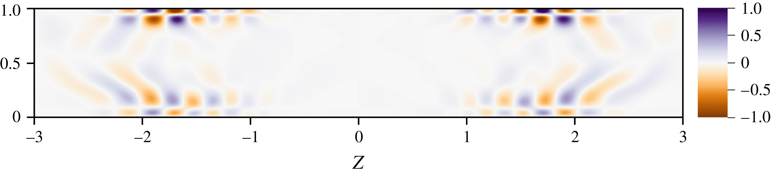
Figure 10 depicts the spanwise velocity field of the adjoint mode associated with the leading eigenmode depicted in figure 9 within the
 $y=-0.5$
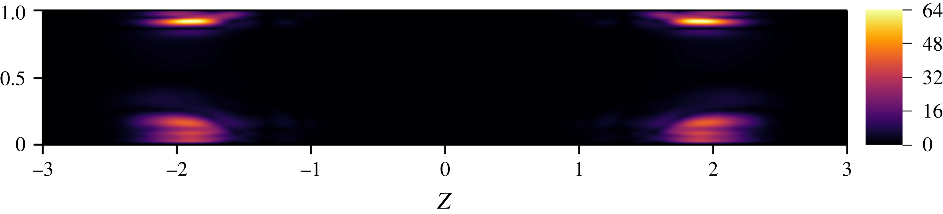
horizontal plane, while the sensitivity of the corresponding growth rate within the same plane is shown in figure 11. Looking at these two figures, it is clear that the secondary instability is mostly sensitive in the vicinity of
 $z=\pm 2$
, while modification within the central part of the cavity (i.e. where the very low-frequency oscillation of the base flow occurs) hardly influences it. Similar results have been obtained for the eigenmode associated with
 $\unicode[STIX]{x1D706}_{3}$
. Along with the very different spatial supports of the primary and secondary instability modes, these sensitivity results strongly justify a posteriori the validity of the frozen base flow assumption used in this section.
Spanwise velocity of the adjoint eigenmode
 $\hat{\boldsymbol{u}}^{\dagger }$
associated with the eigenvalue
 $\unicode[STIX]{x1D706}=0.001\pm \text{i}0.049$
at
 $Re=3800$
in the
 $y=-0.5$
horizontal plane.

Sensitivity to base flow modification
 $\unicode[STIX]{x1D735}_{\boldsymbol{U}}\unicode[STIX]{x1D706}$
of the eigenvector
 $\hat{\boldsymbol{u}}$
associated with the eigenvalue
 $\unicode[STIX]{x1D706}=0.001\pm \text{i}0.049$
at
 $Re=3800$
in the
 $y=-0.5$
horizontal plane. Only the magnitude of real part of
 $\unicode[STIX]{x1D735}_{\boldsymbol{U}}\unicode[STIX]{x1D706}$
is shown, i.e. the sensitivity to base flow modification of the eigenvalue’s growth rate.

5 Discussion
5.1 Comparisons with experiments
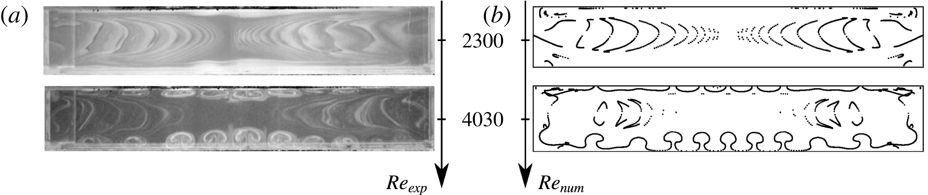
The analyses reported in the previous sections have underlined how the flow can transition from steady state to the emergence of self-sustained periodic oscillations giving rise to a spanwise drift of the Taylor–Görtler-like vortices. Let us now compare the predictions of linear stability analyses and direct numerical simulations against observations obtained using the experimental set-up described in § 2. Figure 12 depicts a visual comparison of the experimental smoke visualizations and the numerically computed streamlines within a horizontal plane cutting through the cavity at two different Reynolds numbers. It is clear that the flow patterns observed experimentally and numerically for the two Reynolds numbers considered are qualitatively similar. As the Reynolds number is increased from
 $Re=2300$
up to
 $Re=4030$
, both the smoke and streamlines visualizations highlight the emergence of mushroom-like structures. These vortical structures are the Taylor–Görtler-like vortices resulting from the different centrifugal instabilities underlined in the previous sections.
Experimental smoke visualization (a) (Faure et al.
Reference Faure, Adrianos, Lusseyran and Pastur2007) and numerically computed streamlines (b). The visualization technique enhances the detection of mushroom-shaped Taylor–Görtler-like vortical structures. Top views in the
 $y=0.8$
plane.

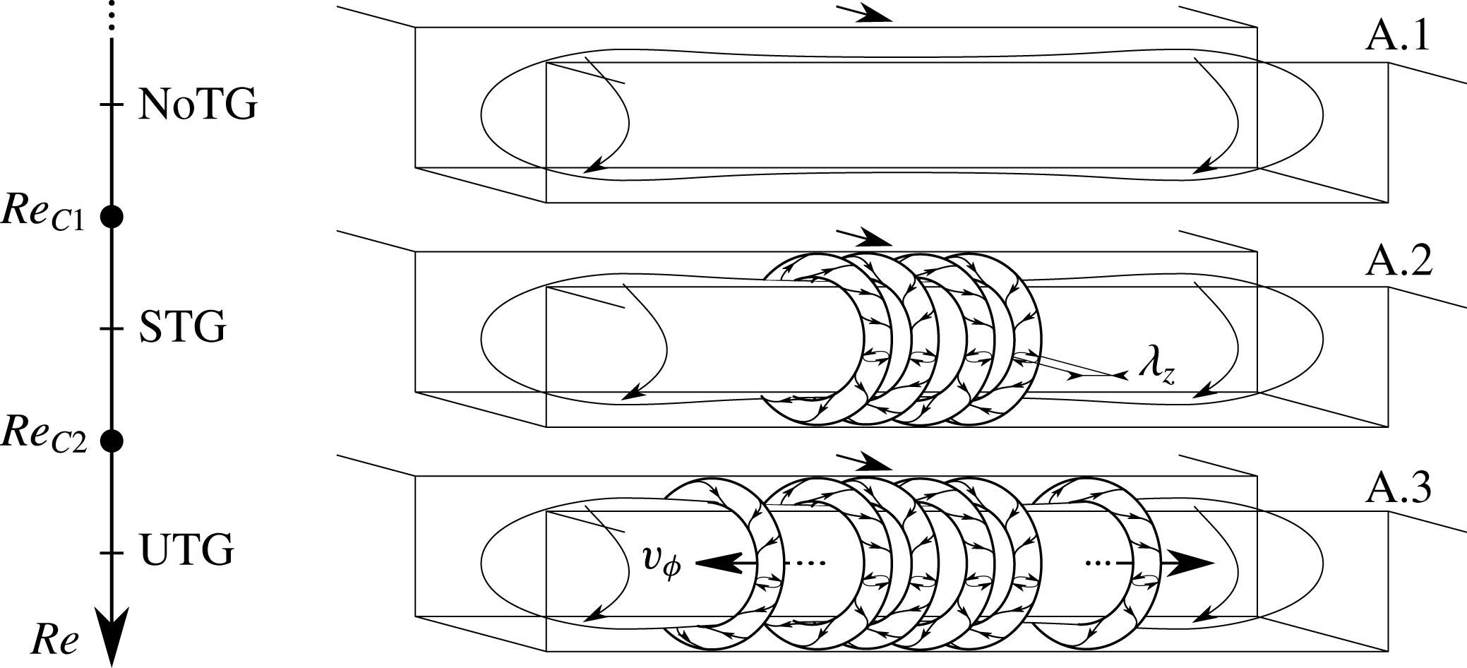
Sketch of the evolution of the morphology of the inner cavity’s flow as a function of the Reynolds number. NoTG, STG and UTG stand for no Taylor–Görtler vortices, (quasi-) stationary Taylor–Görtler vortices and unsteady Taylor–Görtler vortices, respectively.

Summary of the critical Reynolds numbers, spanwise wavelength and circular frequencies observed experimentally, and predicted by linear stability analyses. DNS and GLSA stand for direct numerical simulation and global linear stability analysis, respectively.

Table 4 summarizes the critical Reynolds numbers, wavelengths and circular frequencies observed in our experimental work (see § 2), in direct numerical simulations as well as in our linear stability analyses, while figure 13 provides a schematic representation of the evolution of the flow’s morphology as the Reynolds number increases. As assessed from linear stability analyses, three different flow regimes have been observed. The first one (figure 13
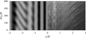
a) is a stationary flow characterized by the absence of Taylor–Görtler vortices and sharing strong similarities with its two-dimensional counterpart. The second flow regime sees the emergence of Taylor–Görtler-like (TGL) vortices localized in the central part of the cavity. Although linear stability analyses predict a stationary flow, direct numerical simulations have revealed that these TGL vortices experience a very low-amplitude and low-frequency oscillation. Such oscillations are extremely difficult to observe owing to their small amplitude and the long time scale over which they take place. Nonetheless, the critical Reynolds number predicted by stability analysis is in extremely good agreement with both direct numerical simulations and experimental observations (only 2 % difference), as is the dominant wavelength of this vortical flow structure. On top of these quasi-stationary TGL vortices, travelling waves are observed in the third flow regime investigated due to the appearance of additional sets of linearly unstable TGL vortices now located in the vicinity of the spanwise end walls. Figure 14 depicts experimental and numerical spatio-temporal diagrams taken along the line
 $(x,y)=(0.1,0.8)$
for
 $Re=3900$
. These diagrams once again highlight the good agreement obtained between the experimental and numerical flow patterns. In both configurations, the central region of the cavity, given by
 $\Vert z/D\Vert <1$
, is mostly dominated by quasi-steady Taylor–Görtler-like vortices characterized by a spanwise wavelength
 $\unicode[STIX]{x1D706}_{z}\simeq 0.5$
. On the other hand, the flow pattern in the outer parts of the cavity, given by
 $\Vert z/D\Vert >1.5$
, is dominated by a right- or left-travelling wave resulting from the instability reported in § 4.1.2. Physically, this travelling wave corresponds to a spanwise drift of the TGL vortices due to the existence of the secondary flow discussed in § 4.1.1 and already investigated experimentally by Faure et al. (Reference Faure, Adrianos, Lusseyran and Pastur2007), Faure et al. (Reference Faure, Pastur, Lusseyran, Fraigneau and Bish2009) Douay (Reference Douay2014) and Douay et al. (Reference Douay, Pastur and Lusseyran2016b
). As for the primary bifurcation, the critical experimental and theoretical critical Reynolds numbers differ by less than 1 %. It has to be noted finally that some small discrepancies exist regarding the oscillation frequency of the lateral TGL vortices. This difference very likely results from small limitations of the experimental set-up highlighted in § 2, namely the existence of a small non-vanishing spanwise component of the incoming flow introducing a systematic bias in the flow direction. Another source of error might reside in the quasi-static assumption made for the secondary base flow. Overcoming this limitation, however, requires the use of Floquet analysis, which is beyond our present capabilities.
Numerical and experimental space–time diagrams of the pattern dynamics at
 $Re=3900$
along the line
 $(x,y)=(0.1,0.8)$
. Streamwise velocity for DNS on the left, experimental smoke visualization on the right. The latter has been rectified using the constant asymmetrical drift velocity obtained for
 $Re_{C1}\leqslant Re\leqslant Re_{C2}$
.

5.2 Influence of the aspect ratio
The results presented so far have been obtained in the case of a relatively large-span square cavity of aspect ratio
 $L\,:\,D\,:\,S=1\,:\,1:6$
, recovering two successive bifurcations leading the flow to transition. Nonetheless, it is not clear yet whether the scenario observed herein might be extended to the flow in open cavities of different aspect ratios. Previous experimental works on square cavities (
 $L/D=1$
, see Faure et al.
Reference Faure, Pastur, Lusseyran, Fraigneau and Bish2009) have shown how the spatial support of the flow instabilities changes drastically when the span to depth ratio,
 $S/D$
, is decreased to values lower than
 $3$
. In these short-span cavities, isolated pairs of vortices are recovered instead of the spanwise rows of centrifugal vortices generally observed for large-span cavities, indicating that the strong spanwise flow induced by the presence of two neighbouring lateral walls may prevent the generation of the centrifugal vortices. However, for cavities having a sufficiently large-span size (
 $S/D\geqslant 3$
), no abrupt change of the main features of the bifurcated flow is observed, the instability modes keeping a very similar shape when
 $S/D$
is increased. In the limit of an infinitely large cavity, a spanwise-homogeneous open cavity flow is obtained, which has been studied numerically by Citro et al. (Reference Citro, Giannetti, Brandt and P.2015a
) for the case
 $L/D=1$
. These authors have shown that the flow undergoes the first bifurcation at a critical Reynolds number of
 $1370$
, the most unstable mode being steady, localized inside the cavity and three-dimensional with spanwise wavelength of approximately
 $0.47$
cavity depths. A structural sensitivity analysis provided by the same authors indicates that, for the considered infinite-span square cavity, the mechanism of generation of the primary unstable mode is completely driven by the recirculating flow inside the cavity. Thus, the primary instability mechanism characterizing an infinite-span square cavity flow appears qualitatively similar to that recovered herein for a large-span cavity, although the critical Reynolds number as well as the dominating wavelengths and shape of the vortical structures are different to those obtained in the present work.
Concerning the case of large-span cavities, Douay (Reference Douay2014) has experimentally investigated their flow dynamics for different aspect ratios. In particular, it has been observed that, for a span ratio
 $S/D=6$
, for any
 $L/D$
ratio, the frequency of the primary bifurcation remains rather low (the associated Strouhal number,
 $St$
, being of order
 $10^{-3}$
), being associated with quasi-steady spanwise-alternated Taylor–Görtler modes. For
 $S/D=12$
, two different behaviours have been recovered depending on the aspect ratio
 $L/D$
. For
 $L/D<1.3$
, the primary modes pertain to the previously mentioned quasi-steady family, whereas for
 $L/D\geqslant 1.4$
, the Strouhal number abruptly increases by one order of magnitude, being associated with propagating modes similar to those previously identified by Bres & Colonius (Reference Bres and Colonius2008), Faure et al. (Reference Faure, Pastur, Lusseyran, Fraigneau and Bish2009), Meseguer-Garrido et al. (Reference Meseguer-Garrido, de Vicente, Valero and Theofilis2014). This indicates that not only the span ratio but also the length ratio may be a critical parameter for the destabilization of open cavity flows, as previously observed in several experimental studies (Gharib & Roshko Reference Gharib and Roshko1987). This is further confirmed by the results recently provided by Liu et al. (Reference Liu, Gómez and Theofilis2016), who performed a global stability analysis on the flow over a long cavity of aspect ratio
 $L\,:\,D\,:\,S=6\,:\,1\,:\,2$
. For
 $Re<1050$
, the leading (although stable) mode is steady and driven by a centrifugal mechanism. This mode is rapidly overtaken by a shear-layer-driven travelling eigenmode, characterized by a relatively high frequency (
 $St\approx 0.23$
), which becomes unstable at
 $Re\approx 1080$
, leading to laminar–turbulent transition. Also for this long cavity, the typical structure of the centrifugal steady mode is reminiscent of the pattern found in previous investigations of spanwise-homogeneous cavity flows (Bres & Colonius Reference Bres and Colonius2008). However, when a spanwise-homogeneous long cavity with
 $L/D=6$
is considered (see Sun et al.
Reference Sun, Nair, Taira, Cattafesta, Bres and Ukeiley2014) no steady modes are recovered in the flow dynamics. This suggests that shear-layer modes may be dominant for long cavities, whereas steady centrifugal ones would prevail in short ones, although modifying the span of the cavity might induce a further change in the flow dynamics. A spanwise-homogeneous approximation might, in some particular cases, succeed at detecting (although qualitatively) the main instability mechanisms driving the flow, but will fail at predicting the critical thresholds for transition as well as the dominant frequencies and wavelengths. This confirms the need of performing global stability analyses for accurately investigating the dynamics of such three-dimensional flows for different aspect ratios.
6 Conclusion
The transition scenario of an incompressible shear-driven cavity flow has been investigated by the joint application of experimental observations, direct numerical simulations and linear stability analyses. Based on the good agreement obtained using these different approaches, a clear scenario is here proposed to explain the transition to unsteadiness. This scenario relies on the occurrence of two successive bifurcations. The first one, happening at a critical Reynolds number
 $Re_{C1}=3430$
, is associated with the emergence of (quasi-)steady Taylor–Görtler vortices. Analysis of the different production terms has revealed the centrifugal nature of the instability, in agreement with previous studies on the two-dimensional shear-driven and lid-driven cavities (Albensoeder et al.
Reference Albensoeder, Kuhlmann and Rath2001). Further increasing the Reynolds number up to
 $Re_{C2}\simeq 3730$
eventually causes a second bifurcation to occur. This second bifurcation is an Andronov–Poincaré–Hopf bifurcation. The flow thus transitions from its quasi-stationary bifurcated state and exhibits self-sustained periodic oscillations. Though a kinetic energy analysis has revealed that the underlying instability is also of centrifugal type, it has to be noted that it nonetheless differs quite significantly from the primary instability. Indeed, while the first instability occurring in the flow is exclusively related to the primary vortex core, the second instability reported in the present work is clearly related to the interplay between the primary vortex core and the existence of the spanwise end walls of the cavity. As a result of this secondary instability, the periodic oscillations of the flow are characterized by a spanwise drift of the vortical structures toward the end walls very likely induced by the existence of the spanwise secondary flow. Although it has been hypothesized in the past (Faure et al.
Reference Faure, Pastur, Lusseyran, Fraigneau and Bish2009; Douay Reference Douay2014) that this drift might result from a global instability of the flow, it is the first time to our knowledge that it has been properly demonstrated by means of fully three-dimensional stability analyses.
Despite linear stability analysis having proved helpful since the early 1900s to gain a better understanding of the fundamental physical mechanisms on which transition to turbulence relies, it fully explains the transition scenario only for a limited number of flow configurations, e.g. Rayleigh–Bénard or the two-dimensional cylinder flow, for instance. Given its wall-bounded nature, it is thus remarkable that linear stability analyses can fully characterize the first two bifurcations taking place in the fully three-dimensional shear-driven cavity flow. Building on this success, our joint experimental and numerical efforts are thus currently aiming at the proper characterization of the second and third bifurcations by means of Floquet analyses. It has to be noted finally that the transition scenario presented in this work is quite different from the one originally proposed by Liu et al. (Reference Liu, Gómez and Theofilis2016) for a similar flow configuration and relying on the emergence of Rossiter-like instability modes. This apparent contradiction, however, results from the significantly different geometry of the cavities considered in these two works. Researchers and engineers willing to pursue this work are thus strongly encouraged to perform parametric studies in order to fully elucidate the influence of the cavity’s dimensions on these transition scenarios.
Acknowledgements
This work was performed using HPC resources from GENCI-[TGCC/CINES/IDRIS] (Grant x20152a6362/x20162a6362). F.L. and L.P. would like to acknowledge Thierry Faure and Panayotis Adrianos for their past contribution to the experimental database. F.P., S.C., J.Ch.L. and J.Ch.R. would like to acknowledge A. Bucci for his help in using the solver Nek5000.