2.1 The Dynamic Stochastic General Equilibrium model

The clash between the two competing business cycle theories—the Real Business Cycle (RBC) perspective (see e.g. King & Rebelo, Reference King and Rebelo1999) and the New Keynesian paradigm (cf. Mankiw & Romer, Reference Mankiw and Romer1991)—ended in the last decade with the development of a NNSFootnote 5. In a nutshell, the canonical model employed by the NNS paradigm is basically a RBC DSGE model with monopolistic competition, nominal imperfections, and a monetary policy rule (see Woodford, Reference Woodford2003; Galí & Gertler, Reference Galí and Gertler2007; Galí, Reference Galí2008, for more detailed expositions of the NNS approach).

In line with the RBC tradition, the starting point of the new vintage models is a stochastic version of the standard neoclassical growth model with variable labor supply: the economy is populated by an infinitely lived representative household, which maximizes its utility under an intertemporal budget constraint, and by a large number of firms, whose homogenous production technology is hit by exogenous shocks. The New Keynesian flavor of the model stems from three ingredients: money, monopolistic competition, and sticky prices. Money has usually only the function of unit of account and its short-run non-neutrality is guaranteed by the nominal rigidities introduced by sticky prices. As a consequence, the central bank can influence the real economic activity in the short run by manipulating the interest rate. The RBC scaffold of the model allows one to compute the ‘natural’ level of output and of the real interest rate, that is, the equilibrium values of the two variables under perfectly flexible prices. The ‘natural’ output and interest rate constitute a benchmark for monetary policy: the central bank cannot persistently push the output and the interest rate away from their ‘natural’ values without creating inflation or deflation. Note that the assumption of imperfect competition (and of other real rigidities) implies that the ‘natural’ level of output is not socially efficient.

Analytically, the NNS model can be represented by three equationsFootnote 6: the expectation-augmented IS equation, the New Keynesian Phillips (NKP) curve, and a monetary policy rule. The expectation-augmented IS equation constitutes the aggregate-demand building block of the NNS model. Assuming perfect capital markets and taking a log-linear approximation around the steady state, one can derive the IS equation from the goods market-clearing condition and the Euler equation of the representative household:

(1)

where is the output gap (i.e. the percentage gap between real output and its ‘natural’ level), σ is the intertemporal elasticity of substitution of consumption, i is the nominal interest rate, π is inflation, r ⁿ is the ‘natural’ interest rate and E_t stands for the expectation operator taken at time t. Note that in line with the traditional IS–LM model, the IS equation postulates a negative relation between the output gap and the interest rate gap.

The aggregate-supply building block of the NNS model boils down to a NKP curve. Starting from the Dixit and Stiglitz (Reference Dixit and Stiglitz1977) model of monopolistic competition and the Calvo (Reference Calvo1983) model of staggered prices (with constant probability of price adjustment), one finds that in any given period firms allowed to adjust prices fix them as a weighted average of the current and expected future nominal marginal cost. The NKP curve can be obtained by combining the log-linear approximation of the optimal price-setting choice, the price index, and the labor–market equilibrium:

(2)

where β is the subjective discount factor of the representative household and κ depends both on the elasticity of marginal cost with respect to output and on the sensitivity of price adjustment to marginal cost fluctuations (i.e. frequency of price adjustment and real rigidities induced by price complementarities). The term u is usually considered a ‘cost-push shock’: it captures the fact that the natural level of output may not coincide with the socially efficient one for the existence of real imperfections such as monopolistic competition, labor market rigidities, etc. The presence of u implies that inflation does not depend only on the presence of a positive output gap, but also on other factors affecting firms’ real marginal costs. (The output gap appears in Equation (2) because in the underlying model there is a positive relation between and the log deviation of real marginal cost from its natural level.)

The model just sketched leads to a system of two difference equations (see Equations (1) and (2)) and three unknowns: the output gap, inflation, and the nominal interest rate. In order to solve the system, one has to append a rule to determine the nominal interest rate. This is the role reserved to monetary policy. The choice of a monetary policy rule is usually carried out adopting a welfare criterion: taking a second-order Taylor series approximation of the utility of the representative household, one can derive a welfare loss function for the central bank that is quadratic in inflation and in deviations of output from its socially efficient level (see Rotemberg & Woodford, Reference Rotemberg and Woodford1999; Woodford, Reference Woodford2003). Even if optimal monetary policy rules could be in principle derived (see e.g. Giannoni & Woodford, Reference Giannoni and Woodford2002a, Reference Giannoni and Woodford2002b), the NNS model is often closed with ‘simple’ rules such as the Taylor (Reference Taylor1993) rule (more on that in Section 2.2.3):

(3)

where i ^τ is the interest rate target of the central bank, φ_y > 0 and φ_π > 1. Before performing policy exercises with the model, one should assess its empirical performance and calibrate its parameters.

When taken to the data (see e.g. Smets & Wouters, Reference Smets and Wouters2003; Christiano et al., Reference Christiano, Eichenbaum and Evans2005), canonical DSGE models like the one presented above are usually expanded to account for investment dynamics. Moreover, different type of shocks are added to both the IS equation, assuming for instance government spending and private consumption disturbances, and the monetary policy rule. Finally, standard DSGE models have also to be modified because they are too much forward-looking to match the econometric evidence on the co-movements of nominal and real variables (e.g. impulse-response functions of output and inflation as to a monetary policy shock). Hence, in order to reproduce the inertia and persistency found in real data, the DSGE models are extended, introducing a great deal of ‘frictions’—often not justified on the theoretical ground—such as predetermined price and spending decisions, indexation of prices and wages to past inflation, sticky wages, habit formation in preferences for consumption, adjustment costs in investment, variable capital utilization, etc.

From an econometric perspective, Equations (1)–(3) of the DSGE model are naturally represented as a vector auto-regression (VAR) model. The estimation of the resulting econometric model is usually carried out either with a limited information approach or by full-information likelihood-based methods.

Limited information approach. The strategy of the limited information approach to estimate and evaluate DSGE models is usually the following (e.g. Rotemberg & Woodford, Reference Rotemberg and Woodford1999; Christiano et al., Reference Christiano, Eichenbaum and Evans2005):

1. 1. Specify the monetary policy rule and the laws of motion for the shocks.

2. 2. Split the parameters in two sets and calibrate the parameters in the first set, providing some theoretical or empirical justifications for the chosen values.

3. 3. Fix the timing of the endogenous variables in order to allow the interest rate to respond to contemporaneous output and inflation, while the latter variables are only affected by lagged interest rate. Under this assumption one can estimate via ordinary least squares (OLS) the coefficients of the monetary policy rule and the impulse-response functions of the three variables to a monetary policy shock.

4. 4. Recover the second set of parameters by minimizing the distance between the model-generated and empirical impulse-response functions.

5. 5. Finally, given the structural parameter values and the VAR, identify the other structural shocks by imposing, if necessary, additional restrictions.

The empirical performance of the model is then measured by comparing the impulse-response functions generated by the model with the empirical ones.

Full information approach. The full information approach was initially discarded to estimate DSGE models because maximum likelihood (ML) methods deliver implausible estimates. However, with the introduction of Bayesian techniques, the full information approach regained popularity and it is now commonly employed (see e.g. Smets & Wouters, Reference Smets and Wouters2003). Bayesian estimation is carried out according to the following steps:

1. 1. Place some restrictions on the shocks in order to allow later identification.

2. 2. Employ the Kalman filter to compute the likelihood function of the observed time series.

3. 3. Form the prior distribution of the parameters by choosing their initial values through calibration, preliminary exploratory exercises, and/or to get some desired statistical properties.

4. 4. Combine the likelihood function with the prior distribution of the parameters to obtain the posterior density, which is then used to compute parameter estimates.

One can then assess the empirical performance of the estimated DSGE model comparing its marginal likelihood with the one of standard VAR models and the model-generated cross-covariances vis-á-vis the empirical ones.

Once one has recovered the parameters of the model by estimation or calibration and has identified the structural shocks, policy-analysis exercises can finally be carried out. More specifically, after having derived the welfare loss function, one can assess the performance of the subset of ‘simple’ policy rules that guarantee the existence of a determinate equilibrium or the more appropriate parametrization within the class of optimal monetary policy rules. This can be done via simulation, by buffeting the DSGE model with different structural shocks and computing the resulting variance of inflation and the output gap and the associated welfare losses of the different monetary policy rules and parameterizations employed (see e.g. Rotemberg & Woodford, Reference Rotemberg and Woodford1999; Galí & Gertler, Reference Galí and Gertler2007). In practice, assuming that the DSGE model is the ‘true’ data generating process of the available time series, one is evaluating how the economy portrayed by the model would react to the same structural shocks observed in the past if the monetary policy followed by the central bank were different.

2.2 Policy with Dynamic Stochastic General Equilibrium models: a safe exercise?

DSGE models are plagued by at least three classes of problems, which could potentially undermine the usefulness of performing policy-analysis exercises in such a framework. More specifically, DSGE models are subject to theoretical, empirical, and political-economy problems that we shall discuss in the next sections.

2.2.2 Empirical issues

The second stream of problems is related to the empirical validation of DSGE models. As remarked by Canova (Reference Canova2008), estimation and testing of DSGE models are performed assuming that they represent the true data-generating process (DGP) of the observed data. This implies that the ensuing inference and policy experiments are valid only if the DSGE model mimics the unknown DGP of the data.

As mentioned in Section 2.1, DSGE models can be represented as a VAR of the form:

(4)

where x are both endogenous and exogenous variables, φ is the vector of the parameters of the model, and E contains the errors. If the matrix A ₀ is invertible, one can obtain a reduced-form VAR representation of the DSGE model.

Following Fukac and Pagan (Reference Fukac and Pagan2006), the econometric performance of DSGE models can be assessed along the identification, estimation, and evaluation dimensions. Before going in depth with this type of analysis, two preliminary potential sources of problems must be discussed. First, the number of endogenous variables contemplated by DSGE models is usually larger than the number of structural shocks. This problem may lead to system singularity and it is typically solved by adding measurement errors. Second, H ₁ and H ₂ are reduced-rank matrixes. This problem is circumvented by integrating variables out of the VAR (Equation (4)), as long as H ₁ and H ₂ become invertible. This process leads to a VARMA representation of the DSGE model. This is not an innocent transformation for two reasons: (i) if the moving average component is not invertible, the DSGE model cannot have a VAR representation; (ii) even if the VAR representation of the DSGE model exists, it may require an infinite number of lags (more on that in Fernandez-Villaverde et al., Reference Fernandez-Villaverde, Rubio-Ramirez and Sargent2006; Alessi et al., Reference Alessi, Barigozzi and Capasso2007; Ravenna, Reference Ravenna2007).

Identification. Given the large number of nonlinearities present in the structural parameters (θ), DSGE models are hard to identify (Canova, Reference Canova2008). This leads to a large number of identification problems, which can affect the parameter space either at the local or at the global level. A taxonomy of the most relevant identification problems can be found in Canova and Sala (Reference Canova and Sala2005)Footnote 8. To sum them up: (i) different DSGE models with different economic and policy implications could be observationally equivalent (i.e. they produce indistinguishable aggregate decision rules); (ii) some DSGE models may be plagued by under or partial identification of their parameters (i.e. some parameters are not present in the aggregate decision rules or are present with a peculiar functional form); (iii) some DSGE may be exposed to weak identification problems (i.e. the mapping between the coefficients of the aggregate decision rules and the structural parameters may be characterized by little curvature or by asymmetries), which could not even be solved by increasing the sample size.

Identification problems lead to biased estimates of some structural parameters and do not allow us to correctly evaluate the significance of the estimated parameters applying standard asymptotic theories. This opens a ridge between the real and the DSGE DGPs, depriving parameter estimates of any economic meaning and making policy analysis exercises useless (Canova, Reference Canova2008). In most of the cases, identification problems can only be mitigated by appropriately re-parameterizing the modelFootnote 9.

Estimation. The identification problems discussed above partly affect the estimation of DGSE models. DSGE models are very hard to estimate by standard ML methods, because ML estimation delivers biased and inconsistent results if the system is not a satisfying representation of the data. This turns out to be the case for DSGE models (see the ‘Evaluation’ section) and it helps to explain why ML estimates usually attain absurd values with no economic meaning and/or are incompatible with a unique stable solution of the underlying DSGE model.

A strategy commonly employed when the DSGE model is estimated following the limited-information approach (cf. Section 2.1) consists in calibrating those parameters hard to identify and then estimating the others. Given the identification problems listed above, Canova (Reference Canova2008) argues that this strategy works only if the calibrated parameters are set to their ‘true’ values. If this is not the case, estimation does not deliver correct results that can be used to address economic and policy questions (see also Canova & Sala, Reference Canova and Sala2005).

As we mentioned in Section 2.1, Bayesian methods are now commonly employed to estimate DSGE models. They apparently solve the problems of estimation (and identification) by adding a (log) prior function to the (log) likelihood function in order to increase the curvature of the latter and obtain a smoother function. However, this choice is not harmless: if the likelihood function is flat—and thus conveys little information about the structural parameters—the shape of the posterior distribution resembles the one of the prior, reducing estimation to a more sophisticated calibration procedure carried out on an interval instead than on a point (see Fukac & Pagan, Reference Fukac and Pagan2006; Canova, Reference Canova2008). Unfortunately, the likelihood functions produced by most DSGE models are quite flat (see e.g. the exercises performed by Fukac & Pagan, Reference Fukac and Pagan2006). In this case, informal calibration is a more honest and internally consistent strategy to set up a model for policy analysis experiments (Canova, Reference Canova2008).

All the estimation problems described above stem also from the fact that DSGE models are not conceived to simplify the estimation of their parameters (Canova, Reference Canova2008). As a consequence, DSGE models put too much stress upon the data, using for instance more unobservable than observable variables (Fukac & Pagan, Reference Fukac and Pagan2006). This requires strong assumptions about the variances in order to get identification and to employ the Kalman filter to obtain the likelihood function. The likelihood functions produced by the Kalman filter are correct only if observations are Gaussian, but macro-economic time series are typically not normally distributed (Fagiolo et al., Reference Fagiolo, Napoletano and Roventini2008).

Evaluation. Evaluating DSGE models means assessing their capability to reproduce as many empirical stylized facts as possible. For instance, following Fukac and Pagan (Reference Fukac and Pagan2006), one can check: (i) whether variables with deterministic trends cotrend; (ii) whether I(1) variables co-integrate and the resulting co-integrating vectors are those predicted by the model; (iii) the consistency (with respect to data) of the dynamic responses (e.g. autocorrelation, bivariate correlations); (iv) the consistency of the covariance matrix of the reduced form errors with the one found in the data; (v) the discrepancies between the time series generated by the model and real-world ones.

Fukac and Pagan (Reference Fukac and Pagan2006) perform such exercises on a popular DSGE model. First, they find that co-trending behaviors cannot be assessed because data are demeaned (a practice commonly followed by DSGE modelers). However, the computation of the technology growth rates compatible with the observed output growth rates shows that the possibility of technical regress is very high. Second, there are no co-integrating vectors, because output is the only I(1) variable. Third, the model is not able to successfully reproduce the mean, standard deviations, autocorrelations, bivariate correlations observed in real data. In addition, the DSGE model predicts the constancy of some ‘great’ ratios such as the consumption-income ratio (in line with the presence of a steady state of the economy), but this is not confirmed by real data. Fourth, many off-diagonal correlations implied by the covariance matrix of the errors are significantly different from zero, contradicting the DSGE model assumption of uncorrelated shocks. Finally, the tracking performance of the model depends heavily on the assumed high serial correlation of the shocks.

The results just described seem to support Favero (Reference Favero2007) in claiming that modern DSGE models are exposed to the same criticisms advanced against the old-fashioned macro-econometric models belonging to the Cowles Commission tradition: they pay too much attention to the identification of the structural model (with all the problems described above) without testing the potential misspecification of the underlying statistical model (see also Johansen, Reference Johansen2006; Juselius & Franchi, Reference Juselius and Franchi2007)Footnote 10. In DSGE models, ‘restrictions are made fuzzy by imposing a distribution on them and then the relevant question becomes what is the amount of uncertainty that we have to add to model-based restrictions in order to make them compatible not with the data but with a model-derived unrestricted VAR representation of the data’ (Favero, Reference Favero2007: 29). There are many signals of the potential misspecification of the statistical model delivered by DSGE models: the presence of many persistent shocks, the fact that theory-free VAR models of monetary policy need to include additional variables such as a commodity price index to match the data, the absurd estimates produced by standard ML estimation, etc. (Fukac & Pagan, Reference Fukac and Pagan2006; Favero, Reference Favero2007). If the statistical model is misspecified, policy analysis exercises lose significance, because they are carried out in a ‘virtual’ world whose DGP is different from the one underlying observed time-series data.

2.3 Any ways out?

Given the theoretical and empirical problems of DSGE models discussed above, the positive economics approach advocated by Milton Friedman would suggest removing or changing the plethora of underlying assumptions in order to improve the performance of the model. As discussed above, this recommendation is reinforced by two related observations. First, the assumptions underlying DSGE models become a sort of straitjacket that precludes the model from being flexible enough to allow for generalizations and extensions. Second, the unrealism of these assumptions prevents policymakers from fully trusting the policy prescriptions developed with DSGE models.

It is far from clear why within the mainstream DSGE paradigm there is a widespread conservative attitude, with no significative attempts to substitute the ‘Holy Trinity’ assumptions of rationality, greed, and equilibrium (Colander, Reference Colander2005), and/or the RBC core, with more realistic ones. For instance, Akerlof (Reference Akerlof2007) argues that a broader definition of agents’ preferences that takes into account the presence of realistic norms can violate many neutrality results of neoclassical economics without resorting to imperfections. Moreover, introducing heterogeneous agents or substituting the rationality assumption with insights coming from behavioral economics could substantially change the working of DSGE models, ‘making monetary policy more of a science’ (Mishkin, Reference Mishkin2007).

In any case, if neoclassical economists truly enlist themselves among those advocating an instrumentalist approach to scientific research, they should agree that when models display estimation and validation (descriptive) problems such as those exhibited by DSGE models, the only way out is to modify the models’ assumptions. A fortiori, this should be the recommendation that an instrumentalist researcher would provide if, in addition, the model, as happens in the DSGE case, also displayed problems on the normative side.

This is exactly the research avenue that a growing number of scholars have been pursuing in the last two decades. Dissatisfied with standard macro-economic, micro-founded, general equilibrium-based neoclassical models like those discussed above, they have begun to devise an entirely new paradigm labeled as ‘Agent-Based Computational Economics’Footnote 12 (ACE). The basic exercise ACE tries to perform is building models based on more realistic assumptions as far as agent behaviors and interactions are concerned, where more realistic here means rooted in empirical and experimental micro-economic evidence. For example, following the body of evidence provided by cognitive psychologists (see, for example, among a vast literature, Kahneman & Tversky, Reference Kahneman and Tversky2000), the assumptions of perfect rationality and foresight are replaced with those of bounded rationality and adaptive behavior. More generally, ACE scholars share the view that agents in the model should have ‘the same information as do the economists modeling the economy’ (Colander, Reference Colander2006a: 11). Similarly, insights from network theory (e.g. Albert & Barabasi, Reference Albert and Barabasi2002) and social interactions (e.g. Brock & Durlauf, Reference Brock and Durlauf2001) suggest moving away from the unrealistic and over-simplifying assumptions concerning agents interactions typically employed in neoclassical models and allowing for direct, non-trivial interaction patterns. Finally, the widespread evidence on persistent heterogeneity and turbulence characterizing markets and economies indicate abandoning crazy simplifications such as the RA assumption, as well as the presumption that economic systems are (and must be observed) in equilibrium, and to focus instead on out-of-equilibrium dynamics, endogenously fueled by the interactions among heterogenous agents.

In other words, ACE can be defined as the computational study of economies thought as complex evolving systems (Tesfatsion, Reference Tesfatsion2006a). Notice that neoclassical economics, on the contrary, typically deals with economies conceived as simple, linear, homogeneous, and stationary worlds. It should not come as a surprise that the class of models used by ACE to explore the properties of markets, industries, and economies (called ABMs) are far more complicated—and harder to analyze—objects than their neoclassical counterparts. In the following section we will therefore begin by outlying the basic building blocks of ABMs. Next, we will address the question how ABMs can be employed to deliver normative implications. Then, we will briefly review some examples of policy exercises in ABMs. Some final remarks about pro and cons of using ABMs for policy analysis will be left for the concluding section.

3.1 Building blocks of agent-based models

The last two decades have seen a rapid growth of agent-based modeling in economics. An exhaustive survey of this vast literature is of course beyond the scope of this workFootnote 13. However, before proceeding, it is useful to introduce the main 10 ingredients that tend to characterize economics AB models.

1. 1. A bottom-up perspective. A satisfactory account of a decentralized economy is to be addressed using a bottom-up perspective. In other words, aggregate properties must be obtained as the macro-outcome of a possibly unconstrained micro-dynamics going on at the level of basic entities (agents). This contrasts with the top-down nature of traditional neoclassical models, where the bottom level typically comprises a representative individual and is constrained by strong consistency requirements associated with equilibrium and hyper-rationality.

2. 2. Heterogeneity. Agents are (or might be) heterogeneous in almost all their characteristics.

3. 3. The evolving complex system (ECS) approach. Agents live in complex systems that evolve through time. Therefore, aggregate properties are thought to emerge out of repeated interactions among simple entities, rather than from the consistency requirements of rationality and equilibrium imposed by the modeler.

4. 4. Nonlinearity. The interactions that occur in AB models are inherently nonlinear. Additionally, nonlinear feedback loops exist between micro- and macro-levels.

5. 5. Direct (endogenous) interactions. Agents interact directly. The decisions undertaken today by an agent directly depend, through adaptive expectations, on the past choices made by other agents in the population.

6. 6. Bounded rationality. The environment in which real-world economic agents live is too complex for hyper-rationality to be a viable simplifying assumption. It is suggested that one can, at most, impute to agents some local and partial (both in time and space) principles of rationality (e.g. myopic optimization rules). More generally, agents are assumed to behave as boundedly rational entities with adaptive expectations.

7. 7. The nature of learning. Agents in AB models engage in the open-ended search of dynamically changing environments. This is due to both the ongoing introduction of novelty and the generation of new patterns of behavior; but also on the complexity of the interactions between heterogeneous agents (see point 5 above).

8. 8. ‘True’ dynamics. Partly as a consequence of adaptive expectations (i.e. agents observe the past and form expectations about the future on the basis of the past), AB models are characterized by true, non-reversible dynamics: the state of the system evolves in a path-dependent mannerFootnote 14.

9. 9. Endogenous and persistent novelty. Socio-economic systems are inherently non-stationary. There is the ongoing introduction of novelty in economic systems and the generation of new patterns of behavior, which are themselves a force for learning and adaptation. Hence, agents face ‘true (Knightian) uncertainty’ (Knight, Reference Knight1921) and are only able to partially form expectations on, for instance, technological outcomes.

10. 10. Selection-based market mechanisms. Agents typically undergo a selection mechanism. For example, the goods and services produced by competing firms are selected by consumers. The selection criteria that are used may themselves be complex and span a number of dimensions.

3.2 The basic structure of agent-based models

Models based on (all or a subset of) the 10 main ingredients discussed above typically possess the following structure. There is a population—or a set of populations—of agents (e.g. consumers, firms, etc.), possibly hierarchically organized, whose size may change or not in time. The evolution of the system is observed in discrete time steps, t = 1,2…. Time steps may be days, quarters, years, etc. At each t, every agent i is characterized by a finite number of micro-economic variables (which may change across time) and by a vector of micro-economic parameters (that are fixed in the time horizon under study). In turn, the economy may be characterized by some macro-economic (fixed) parameters Θ.

Given some initial conditions and a choice for micro- and macro-parameters, at each time step t > 0 one or more agents are chosen to update their micro-economic variables. This may happen randomly or can be triggered by the state of the system itself. Agents selected to perform the updating stage collect their available information about the current and past state (i.e. micro-economic variables) of a subset of other agents, typically those they directly interact with. They plug their knowledge about their local environment, as well as the (limited) information they can gather about the state of the whole economy, into heuristics, routines, and other algorithmic, not necessarily optimizing, behavioral rules. These rules, as well as interaction patterns, are designed so as to mimic empirical and experimental knowledge that the researcher may have collected from his/her preliminary studies.

After the updating round has taken place, a new set of micro-economic variables is fed into the economy for the next-step iteration: aggregate variables are computed by simply summing up or averaging individual characteristics. Once again, the definitions of aggregate variables closely follow those of statistical aggregates (i.e. GDP, unemployment, etc.).

The stochastic components possibly present in decision rules, expectations, and interactions will in turn imply that the dynamics of micro- and macro-variables can be described by some (Markovian) stochastic processes parameterized by micro- and macro-parameters. However, nonlinearities which are typically present in decision rules and interactions make it hard to analytically derive laws of motion, kernel distributions, time-t probability distributions, etc. for the stochastic processes governing the evolution of micro- and macro-variables.

This suggests that the researcher must often resort to computer simulations in order to analyze the behavior of the ABM at hand. Notice that in some simple cases such systems allow for analytical solutions of some kind. Needless to say, the more one injects into the model assumptions sharing the philosophy of the building blocks discussed above (cf. Section 3.1), the less tractable turns out to be the model, and the more one needs to resort to computer simulations. Simulations must be intended here in a truly constructive way, for example, to build and ‘grow’ a society ‘from the bottom up’, in the spirit of object-oriented programming.

3.3 Descriptive analysis of agent-based models

When studying the outcomes of ABMs, the researcher often faces the problem that the economy he/she is modeling is by definition out-of-equilibrium. The focus is seldom on static equilibria or steady-state paths. Rather, the researcher must more often look for long-run statistical equilibria and/or emergent properties of aggregate dynamics (that is, transient statistical features that last suffficiently long to be observed and considered stable compared with the time horizon of the model; see Lane, Reference Lane1993a, Reference Lane1993b for an introduction). Such an exploration is by definition very complicated and it is made even more difficult by the fact that the researcher does not even know in advance whether the stochastic process described by its ABM is ergodic or not and, if it somehow converges, how much time will take for the behavior to become sufficiently stable.

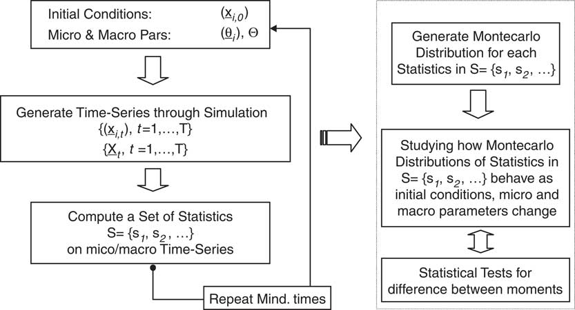
Suppose for a moment that the modeler knows (e.g. from a preliminary simulation study or from some ex-ante knowledge coming from the particular structure of the ABM under study) that the dynamic behavior of the system will become sufficiently stable after some time horizon T* for (almost all) points of the parameter space. Then a possible procedure that can be implemented to study the output of the ABM runs as the one synthetically depicted in Figure 1.

Figure 1

A schematic procedure for studying the output of an agent-based model

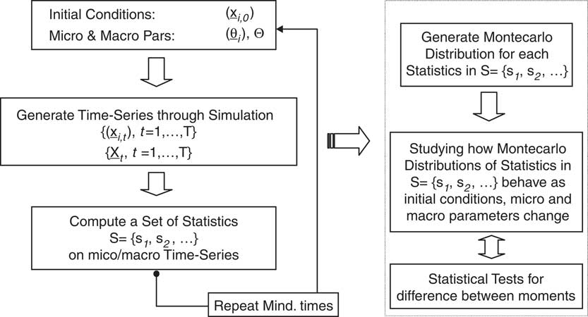
Given some choice for initial conditions, micro-, and macro-parameters, assume we run our system until it relaxes to some stable behavior (i.e. for at least T > T * time steps). Suppose we are interested in a set S = {s ₁, s ₂, …} of statistics to be computed on micro- and macro-simulated variables. For any given run the program will output a value for each statistic. Given the stochastic nature of the process, each run will output a different value for the statistics. Therefore, after having produced M independent runs, one has a distribution for each statistic containing M observations, which can be summarized by computing its moments.

Recall, however, that moments will depend on the choice made for initial conditions and parameters. By exploring a sufficiently large number of points in the space where initial conditions and parameters are allowed to vary, computing the moments of the statistics of interest at each point, and by assessing how moments do depend on parameters, one might get a quite deep descriptive knowledge of the behavior of the system (see Figure 1).

3.4 Model selection and empirical validation

From the foregoing discussion it clearly emerges that in agent-based modeling (as in many other modeling endeavors) one often faces a trade-off between descriptive accuracy and explanatory power of the model. The more one tries to inject ‘realist’ assumptions into the model, the more complicated the system becomes to study and the less clear the causal relations going from assumptions to implications are. ABM researchers are well aware of this problem and have been trying to develop strategies to guide the process of assumption selection. For example, one can try to solve the trade-off between descriptive capability and explanatory power either by beginning with the most simple model and complicating it step-by-step (i.e. the so-called KISS strategy, an acronym for ‘Keep It Simple, Stupid!’) or by starting with the most descriptive model and simplifying it as much as possible (i.e. the so-called KIDS strategy, ‘Keep It Descriptive, Stupid!’). A third, alternative strategy prescribes starting instead with an existing model and successively complicating it with incremental additions (this strategy might be labeled TAPAS, for ‘Take A Previous model and Add Something’).

In all these procedures, the extent to which the ABM is able to empirically replicate existing reality should play a crucial role in discriminating the point at which any procedure should stopFootnote 15.

Notice that the very structure of ABMs naturally allows one to take the model to the data and validate it against observed real-world observations. Indeed, an ABM can be thought of as providing a family of DGPs, which we think real-world observations being a realization of. More precisely, let us suppose that we believe that observed data are generated by an unknown (to us) colossal DGP, with an almost infinite number of parameters, which we can label as real-world DGP (rwDGP). Suppose further that such rwDGP can be broken in reasonable smaller weakly exogenous components, each one with a reasonable number of parameters, and each one describing a small set of variables that we are interested in, on the basis of a small set of other variables. Building an ABM means attempting to approximate one of those small rwDGPs. Due to its stochastic structure, an ABM actually mimics the small rwDGP we are studying by a theoretical DGP that generates the same variables each time we run the model. Of course, we only have one observation generated by the rwDGP, and this makes any inference very difficult (but this has to do with another story, which philosophers call the problem of induction)Footnote 16.

Many approaches to empirical validation (and selection) of ABMs can be in principle taken, and the debate is very open here. For example, one might select among ABMs (and within different parameter setups of the same ABM) with respect to the number of stylized facts each of them is able to jointly replicate. A typical procedure to be followed starts with asking whether a particular model can simultaneously reproduce some set of stylized facts for a given parametrization (a sort of ‘exercise in plausibility’); then explore what happens when the parameter setup changes; finally, investigate if some meaningful causal explanation can be derived out of that step-by-step analysis. Alternatively, one can first select among parameters by calibrating the model (e.g. by directly estimating parameters, when possible, with micro- or macro-data) and then judge to what extent the calibrated model is able to reproduce the stylized facts of interest. Notice that, unlike economists supporting the NNS approach—who hold strong theoretical priors rooted in the DSGE model—ACE scholars are more interested in developing plausible theories, which however are not dogmatically deemed to be the ‘correct’ ones (on this point, see also Colander, Reference Colander2006a).

No matter which empirical validation procedure is actually employed, its basic goal is often to restrict the size of the set of free parameters. In fact, over-parameterized models are difficult to interpret and analyze, because no one knows whether the same conclusions could have been obtained in a simpler, less parameterized model. Even if empirical validation allows one to restrict the set of free parameters to a reasonably sized one, many methodological problems still remain when the model is used to perform policy experiments. If any parametrization represents an alternative world, which one should be employed to assess policy performance? What is the role of initial conditions? We shall briefly return to these issues in the concluding remarks.

3.5 Policy experiments in agent-based models: some considerations

ABMs configure themselves as a very powerful device to address policy questions in more realistic, flexible, and modular frameworks. Indeed, as far as economic policy is concerned, ABMs have many advantages as compared with such neoclassical tools as the DSGE model, which we organize in what follows into two classes: theory and empirics.

Theory. ABMs, contrary to neoclassical ones, do not impose any strong theoretical consistency requirements (e.g. equilibrium, representative individual assumptions, rational expectations). This is because they are not required ex-ante to be analytically solvable. Such a no-straitjacket condition allows for much higher flexibility in model building. If this is coupled with a serious empirical-validation requirement (see below), we are in the presence of a semi-instrumentalist approach, where bad (but empirically plausible) assumptions can be replaced with better (and empirically plausible) ones if the model does not perform as expected. Notice also that in the absence of strong consistency conditions, assumptions can be replaced in a modular way, without impairing the analysis of the model. Indeed, in standard neoclassical models one cannot simply replace the optimization assumption with another one just because the model does not behave well, as that would possibly destroy its analytical solvability. This is not so in ABMs: assumptions—or simply small elements of them—can be taken out of the shelf and easily implemented in the model thanks to the flexibility of computer programming languages.

Empirics. As discussed above, ABMs can be thought as stochastic generators of alternative worlds, that is, theoretical DGPs that approximate the unknown one. Contrary to neoclassical models, the structure of ABMs allows us more easily to take them to the data. This can be done in two ways. First, one can validate the inputs of ABMs, that is, fine-tune modeling assumptions about individual behaviors and interactions to make them more similar to the observed ones. Second, one can validate the model on the output side, for example, by restricting the space of parameters, individual behaviors and interactions, and initial conditions to those that allow the model to replicate the stylized facts of interest. This allows for a degree of realism that is much higher than that exhibited, for example, by DSGE models. Furthermore, thanks to the theoretical flexibility discussed above, the set of stylized facts that one can target can include more than one piece of evidence, as instead happens in neoclassical models. In other words, each neoclassical model is typically build—in order to retain analytical solvability—to explain one or two single stylized facts (see the discussion in Aoki, Reference Aoki2006, for more details). On the contrary, each ABM can easily explain a great deal of pieces of empirical evidence.

But how can one actually conduct policy experiments in ABMs? In a very natural way, indeed. Take again the procedure for ABM descriptive analysis outlined in Figure 1. Recall that micro- and macro-parameters can be designed in such a way to mimic real-world key policy variables like tax rates, subsidies, interest rates, money, etc. and other key behavioral measures affecting individual incentives in growth, innovation, or technologically related policies. Moreover, initial conditions might play the role of initial endowments and therefore describe different distributional setups. In addition, interaction and behavioral rules employed by economic agents can easily be devised so as to represent alternative institutional, market, or industry setups. Since all these elements can be freely interchanged, one can investigate a huge number of alternative policy experiments and rules, the consequences of which can be assessed either qualitatively or quantitatively (e.g. by running standard statistical tests on the distributions of the statistics in S). For example, one might statistically test whether the effect on the moments of the individual consumption distribution (the average, etc.) will be changed (and if so by how much) by a percentage change in any given consumption tax rate. Most importantly, all this might be done while preserving the ability of the model to replicate existing stylized facts, for example, some time-series properties of observed aggregate variables (e.g. persistence of output growth-rate fluctuations) or some relation existing between them (e.g. a Phillips curve).

3.6 Policy in agent-based models: a telegraphic survey

The extreme flexibility of ACE modeling has recently motivated researchers to extensively use these approach to address economic policy experimentsFootnote 17. A general trend that can be observed is that political decision makers seems more and more willing to believe in findings based on rather detailed simulation models (such as ABMs), where they see a lot of the economic structure they are familiar withFootnote 18, rather than in general insights obtained in quite abstract mathematical models (such as DSGE models).

The number of ABM models that have been recently addressing policy issues is becoming so large that it would be impossible to survey them in a single paper section. We shall therefore outline in a telegraphic way the main fields where these exercises have been performed and briefly discuss some specific examples. It must be noted from the beginning, however, that despite its increasing success, policy-oriented ABM exercises are still far from generating a robust simulation framework able to address, together, issues related to short-term business cycles, fiscal, and monetary policy (see Dosi et al. (Reference Dosi, Fagiolo and Roventini2010) for a first step in this direction). Therefore, we have chosen to survey here ABM policy-exercises characterized by different aims and focuses, whose policy implications are not always comparable with those of DSGE models.

Industrial policy and market design. ABMs offer a unique possibility for evaluating from a comparative perspective alternative policies and institutional changes in rather specific models of particular economic environments, such as particular markets and/or industries, specific auction types, etc. Indeed, the modeler can tailor his/her ABM so as to precisely mimic a particular instance of the system of interest, by designing individual behaviors, interaction rules, institutional, and technological setups so as to match any empirical or anecdotal knowledge. Examples include detailed models of the U.S. coffee market (Midgley et al., Reference Midgley, Marks and Cooper1997) or the pharmaceutical industry (Malerba & Orsenigo, Reference Malerba and Orsenigo2002). Along similar lines, Malerba et al. (Reference Malerba, Nelson, Orsenigo and Winter2008) extend their previous work on ‘history-friendly’ modeling of the evolution of the computer and the semiconductor industry and use their developed simulation model to study the effect of different types of policies (e.g. antitrust policies, entry-support policies or public procurement on the evolution of industry concentration, and the rate of technological change). The emergence of different types of bidding behavior in different market environments is instead the main topic of Duffy and Unver (Reference Duffy and Unver2008). They simulate the behavior of bidders in two types of auctions—hard or soft close auctions—that differ with respect to the rule governing when the auction is closed. The model is able to reproduce the stylized facts observed in real-world internet auctions and, in addition, offers interesting insights into the features of the bidding functions responsible for the resulting payoffs. The implications for market design are therefore very importantFootnote 19. Sun and Tesfatsion (Reference Sun and Tesfatsion2007) focus instead on the very exciting and promising area of market design. They report on the development and implementation of an ABM framework (called AMES) for testing the dynamic efficiency and reliability of the Wholesale Power Market Platform (WPMP, i.e. a market design proposed by the U.S. Federal Energy Regulatory Commission for common adoption by all U.S. wholesale power markets). As stated by the authors, AMES ‘models strategic traders interacting over time in a wholesale power market that is organized in accordance with core WPMP features and that operates over a realistically rendered transmission grid’. The usefulness of the AMES framework is illustrated in the paper by presentation of a simple static five-node transmission grid test case. AMES provides an exemplar in its detailed specification and the use of open-source software that opens up the door for replication and detailed verification by the ABM community.

Fiscal policy. The assessment of the impact of labor market policies at both the aggregate and individual levels is addressed in Neugart (Reference Neugart2008), who develops a multi-sector agent-based model where firms belonging to different sectors require workers with different skills. Using his ABM, Neugart shows that government-financed training measures increase the outflow rate from unemployment, but reduce the outflow rate for those who do not receive subsidies. Therefore, although at the aggregate level the unemployment rate decreases, at the individual level this labor market policy may harm workers who do not receive government transfersFootnote 20. Mannaro et al. (Reference Mannaro, Marchesi and Setzu2008) look instead to financial markets and develop an ABM populated by behaviorally heterogeneous traders with limited resources. They challenge the idea that a Tobin tax is able to stabilize foreign exchange and stock markets, and to reduce speculation. Their simulations show that Tobin-like taxes may actually increase volatility and decrease trading volumesFootnote 21. Russo et al. (Reference Russo, Catalano, Gallegati, Gaffeo and Napoletano2007) develop an ABM where transactions on the good and labor markets take place through bilateral bargaining occurring between heterogenous firms and consumers/workers. Besides reproducing many micro- and macro-regularities (e.g. sustained growth and fluctuations, Beveridge, Phillips, and Okun curves, etc.), they use the model as a computational laboratory and find that aggregate output is non-monotonically linked to the level of the tax rate levied on corporate profits if revenues are employed to finance R&D investment, whereas output is negatively affected if the money collected through taxes is used to provide unemployment benefits.

Growth policy. Dosi et al. (Reference Dosi, Fagiolo and Roventini2010) study a broad set of normative issues regarding the impact of alternative technological and knowledge scenarios on the rates of growth, innovation, and imitation of a given country. To do so, they build upon their previous model of endogenous growth and business cycles (Dosi et al., Reference Dosi, Fagiolo and Roventini2006) and develop a broader, modular, agent-based frameworkFootnote 22. They show that this broader model is even able to robustly replicate a higher number of stylized facts than its ‘ancestor’ concerning macro-economic dynamics (e.g. cross-correlations, relative volatilities) as well as micro-economic dynamics (e.g. firm size distributions, firm productivity dynamics, firm investment patterns). Furthermore, they define different technological scenarios (e.g. exogenous or endogenous technology frontier, imitation). Finally, they study the long-term impact of a range of different policies considering long-run GDP growth rates, GDP growth-rate volatility, and unemployment. Their results show that: (i) patents appear to be detrimental to growth and to increase unemployment; (ii) imitation spurs GDP growth especially in the endogenous technology frontier scenario; (iii) increasing the expected productivity of entrant firms raises GDP long-run growth in the endogenous technology frontier scenario; and (iv) Keynesian demand macro-management policies are a necessary condition for robust GDP growth and reduced business cycle fluctuations. More generally, the results of Dosi et al. (Reference Dosi, Fagiolo and Roventini2010) point to an existing complementarity between Keynesian policies affecting demand and Schumpeterian policies affecting innovationFootnote 23.

Social interactions. Given the importance of direct interaction in ABMs, many authors have explored the impact of alternative network structures and dynamics upon aggregate outcomes. For example, Carayol et al. (Reference Carayol, Roux and Yildizoglu2008) study how properties of networks that emerge due to uncoordinated individual link formation decisions compare with those of efficient networks. Based on their insights, policies might be designed with the goal of fostering the emergence of efficient networks. Wilhite and Allen (Reference Wilhite and Allen2008) explore the impact of several anti-crime policies dynamically undertaken in societies composed of heterogenous interacting agents. The model is able to explain several real-world patterns concerning the emergence and distribution of crime, and the intertemporal behavior of criminals. For example, larger cities are shown to develop higher crime rates because larger populations increase the incentives to free-ride on public goods. Furthermore, despite crime decreases with protection spending, the impact of prison turns out to be ambiguous, as a higher rate of imprisonment may lead to more crime in the long run.