INTRODUCTION
In recent decades, cattle farms in France have seen their individual area increase while the workforce has remained stable (55 ha and 1·8 Annual Work Unit (AWU) in 2000 as against 69 ha and 1·8 AWU in 2007 on average for dairy cattle farms; Agreste 2008). The reduction in the available workforce per hectare has meant a gain in hourly productivity, obtained notably by mechanization, as observed in Dutch agriculture (Meerburg et al. Reference Meerburg, Korevaar, Haubenhofer, Blom-Zandstra and Van Keulen2009). However, livestock farmers have to manage increasingly wide-spread field patterns, with areas that are ever more diverse and distant from each other. The field characteristics now identified as restricting their use are: distance to the farmstead, area, slope and altitude. Distance, associated with the field area, is a key element in the allocation of a field to grazing by milked cows going to the milking parlour twice a day (Morlon & Benoit Reference Morlon and Benoit1990; Brunschwig et al. Reference Brunschwig, Josien and Bernhard2006; Andrieu et al. Reference Andrieu, Josien and Duru2007). Slope and altitude are determinants of the use of fields in mountainous areas (Fleury et al. Reference Fleury, Dubeuf and Jeanin1996; Andrieu et al. Reference Andrieu, Josien and Duru2007). There are often combined constraints on the fields of mountain farms, reducing the range and seasonality of possible uses. The frequency and extent of climatic uncertainties also increasingly complicate the management of forage production and grazing (Baumont et al. Reference Baumont, Deux, Farruggia and Jouven2008; Mosnier et al. Reference Mosnier, Agabriel, Lherm, van Itterson, Wolfe and van Laar2009). These constraints are determinants of the spatio-temporal utilization of fields and have consequences on structural charges and forage self-sufficiency as well as on the environment at farm level (e.g. biodiversity and nitrate leaching) (Andrieu et al. Reference Andrieu, Josien and Duru2007; Sorel et al. Reference Sorel, Viaud, Durand and Walter2010; Houlbrooke et al. Reference Houlbrooke, Paton, Littlejohn and Morton2011). So better account must be taken of field geographical characteristics in the management of forage areas to improve the way these farms function. To respond to this issue, researchers must propose new management methods for the forage system, in particular models of the way livestock farms function must take the spatial and temporal organization of field use into account. Thus, Martin et al. (Reference Martin, Hossard, Theau, Therond, Josien, Cruz, Rellier, Martin-Clouaire and Duru2009) published ‘an expert-based discrimination tree of grassland use opportunities’ in the spring to identify the conditions of flexibility in grassland use to accommodate unexpected events. To contribute to this discussion, the objective of the present study was to characterize the types of grassland use in a mountain cattle farm system and link them to the geographical characteristics of the fields to derive a conceptual model of grassland. Such a model, incorporated into a whole beef and/or dairy farm model (e.g. Jouven & Baumont Reference Jouven and Baumont2008), would simulate the impact of practice changes on production and positive and negative environmental impacts (e.g. carbon sequestration and nitrate leaching) according to the fields' geographical characteristics. The whole grazing season in mountain grassland cattle farms, which are particularly confronted by constraints to mechanization and animal transport such as slope and distance to farmstead, was considered. This approach was focused on the traditional Salers system, located in a mountainous area of the Massif Central and based on the mixed production (dairy and store animals) of cows of the Salers breed.
MATERIALS AND METHODS
Surveys were performed in farms and a database constructed at field level combining data on geographical characteristics, practices and their seasonality for forage production and utilization (cutting and grazing) and forage supply at pasture.
Description of the traditional Salers livestock system
The traditional Salers livestock system is a typical mountain bovine system located in the mountainous area of the Massif Central, France (Cantal and Puy-de-Dôme departments). These farms manage a dual-purpose herd (milk and store cattle production) and frequently a suckler herd on the same field pattern. This system uses the hardy Salers breed for simultaneous production of milk and store animals. In this system, the calf initiates milking and suckles after milking, which makes both milk production and calf development possible. This type of traditional system and milking was widely encountered in mountainous areas of France, the Andes and the Himalayas as described by Teissier (Reference Teissier1979). This system was selected for its mountainous location and for its management of both dairy and suckling herds that necessitates dealing with constraints encountered in both dairy and beef systems.
The survey
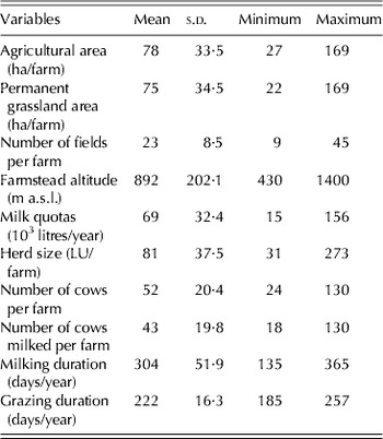
The aim was to investigate the largest possible proportion of the population of traditional Salers farms: 72 farmers participated in the survey, corresponding to 0·8 of the 90 farms in 2005. Their farms are of medium size (78 ha) and number of cows (43) (Table 1), but low milk quotas (69 000 litres/year) compared to the average value in France (40 cows with 254 000 litres of milk collected per farm and per year; Institut de l'Elevage 2008). Milking duration is highly variable, from 135 to 365 days per year (Table 1). Mean altitude corresponds to mountainous elevation with a wide range of variation; farmsteads are located from 430 to 1400 m a.s.l. The farms investigated were typically grass-based systems with all of the agricultural area under permanent grassland; the grazing duration is on average 7·5 months. Among the sample, 43 farms managed a dual-purpose herd and 29 farms managed both a dual-purpose herd and a suckler herd.
Description of the farms included in the dataset

Data were collected during one visit to each farmer in 2005 (Agabriel et al. Reference Agabriel, Sibra, Journal and Coulon2005) by students of VetAgro Sup (National School for Agronomy Engineers) located at Clermont-Ferrand, France. The data related to the farming system (Table 1), animal production and forage management. At the farm level, information was obtained about herd composition, animal grouping, feeding supply (forage and concentrate) per group throughout the year and the total quantities of conserved forage produced and bought. In the present study, a field corresponds to the smallest functional and spatial unit (Thenail & Baudry Reference Thenail and Baudry2004) with homogeneous land use in 2005. For example, a field with a grazing sequence on half of its area and simultaneously a cutting on the other half was considered here as two fields. Each field (n=1586) was geographically characterized by the farmer: area, distance to farmstead, slope, altitude and bearing capacity of the soil. Values obtained for area were validated with official measurements (aerial photographs). The farmer indicated the area of the field with low bearing capacity and with medium or severe slope, according to his own perception. The information on the perception of the farmer was expected to have higher correlation with grassland use than measured variables. A detailed cutting and grazing schedule was created for each field, including all the cutting dates, the type of conserved forage harvested, the entrance and exit dates of animal groups and the quantity of forage supplied at grazing. Fields that were cropped (n=23), used by other farmers (n=28) or abandoned (n=35) were not included in the study.
Construction of the variables
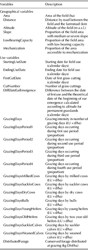
All the geographical and utilization variables used in the present study are reported in Table 2. Seasonality of field use was considered by dividing the grazing season into four periods. The first period, from turnout to 22 May, corresponds to the topping period (early and short grazing before cutting). The second period, 23 May–5 August, corresponds to spring grazing. The third period, 6 August–21 September, corresponds to summer grazing after first cutting and the fourth period, 22 September to turn-in, corresponds to autumn grazing. These dates were calculated respectively as the average dates for the end of first grazing (for fields where grazing is the first use), for the first overall grazing area enlargement (start of grazing after first cutting on cut and grazed fields), and for the second overall grazing area enlargement. Consequently, the first and second periods correspond basically to the first cycle, the third period to the second cycle and the fourth period to the third cycle (Jouven & Baumont Reference Jouven and Baumont2008).
Geographical and use variables investigated

To account for the specificity of the traditional Salers system, field use by milked cows, dry cows (Dcow) and suckler cows (Scow) was considered. Calves were either suckler or weaned calves. Grazing by young heifers (1–2 years old), old heifers (2–3 years old), bulls and equines was also mentioned. The value of each animal category was adapted from the EU livestock units (LU) by expert knowledge (G. Liénard, personal communication). This definition accounts for the diversity of young animal categories (calves, young and old heifers) and allows comparisons between fields, whatever the relative contribution of each animal category: 1 LU for milked cows, 0·85 LU for Scow and Dcow, 0·15 LU for suckler calves, 0·35 LU for weaned calves, 0·55 and 0·75 LU for young and old heifers, respectively. Thus, a milked cow–calf pair was considered as 1·15 LU. A value of 1 LU was fixed for bulls and equines. The grazing intensity variable was constructed to account for both the stocking rate and the duration of its application on the field, i.e. it was calculated per period and per type of animal as the number of LU per ha multiplied by the number of grazing days (LU×d/ha). These variables were also calculated together in a global grazing intensity for the whole grazing season and all the animals (GrazingDays, Table 2). From the feeding supply, registered in kg dry matter (DM) per head and per day, each field was also characterized by the total quantity of forage distributed during the grazing season (in kg DM/ha).
First use, either cutting or grazing, was characterized by its precocity relative to the theoretical date of the beginning of ear emergence, which corresponds to the average date for ear emergence in permanent grassland. It was calculated according to altitude for permanent grasslands, assuming a date of 120 calendar days after 1 January at 400 m a.s.l. and an increase of six days per increase of 100 m of altitude (Réseaux d'élevage Auvergne et Lozère 2006). This variable evaluates the grass development stage and its quality, relative to ear emergence, at the time of first use.
Milk production per cow was not available because in the traditional Salers system, milk is successively sucked by the calf and milked at each milking. Also, it was not possible to register forage production per field because farmers record harvesting over several fields.
Data analysis
The overall approach used in the present work characterized grassland use, in relation to field geographical characteristics, and consisted of two types of analyses. First, a field use typology was constructed from multivariate data analyses. Secondly, the ways in which the geographical characteristics vary according to field use classes were tested. The field was considered as the statistical individual.
Initially, three general field uses were identified and so field use typologies were obtained separately for three field groups, i.e. on cut only (C, n=113), cut and grazed (CG, n=679) and grazed only fields (G, n=794). This distinction was motivated by the different sets of relevant variables between these groups, some variables characterizing grazing practices and the others characterizing cutting practices. For each of these groups, a principal component analysis (PCA) was applied on variables related to cutting and/or grazing practices and their seasonality (SPAD 2005). Some redundant quantitative variables were removed according to the correlations obtained from the PCAs. The resulting principal components or factors were subjected to a hierarchical cluster analysis (SPAD 2005). This method classifies fields that are similar to each other but different from others by maximizing intra-group homogeneity and inter-group diversity, as mentioned by Gaspar et al. (Reference Gaspar, Escribano, Mesias, Rodriguez de Ledesma and Pulido2008). The number of clusters was proposed by the scree test (Cattell Reference Cattell1966) available in SPAD. The classifications obtained were verified and described with a linear mixed model analysis testing the effect of the field use classes on the variables related to grassland use. In this case, the mixed model methodology accounted for the random effect of the farm (Proc Mixed, SAS®2000) and enabled general and robust relationships to be established, whatever the field pattern. The relationships between the geographical characteristics and the field groups were studied independently of the field pattern. Differences between (1) the field groups (C, G and CG) and (2) the field use classes in each group in terms of distance to the cowshed, area, altitude and proportion of the area with low bearing capacity were tested with linear-mixed models including the farm as a random factor. Prior to the mixed model analyses, all the proportion variables were subjected to an angular transformation (square root of the arcsine) to cope with the hypotheses of normal distribution and homogeneity of variances (Sokal & Rohlf Reference Sokal and Rohlf1995).
All the statistical analyses were performed with an unbalanced design, i.e. with different numbers of data between the classes and with some missing data on some geographical characteristics. Consequently, it is not possible to consistently represent the significant differences between means by a constant error terms because the heterogeneity is reflected in the standard errors of means and differences (Piepho Reference Piepho2000). Thus the similarities and differences have been indicated in the results presented using letters (by permission of the JAS Editors, since this is not usually accepted in this Journal).
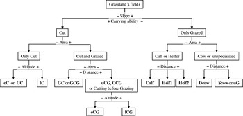
Then a conceptual model of grassland use was constructed using the significant differences observed between the field use classes, in terms of geographical determinants. This model corresponds to a discrimination tree that first separates the three field groups (C, CG and G), then divides into field use classes. Each branch was characterized by its geographical determinant(s).
RESULTS
Description of the fields
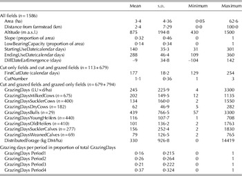
The geographical characteristics of the 1586 fields surveyed are described in Table 3. Average altitude and proportion of the area with slope correspond to a European upland agricultural area. Maximum and minimum values for altitude and distance to farmstead are consistent with the existence of summer mountain pastures. Area and the proportion of the area with low bearing capacity were also very variable. The dataset was consequently characterized by a mix of more useful fields but also fields that were restrictive in terms of suitability for mechanization and/or grazing.
Field use and geographical characteristics

The description of the field use characteristics (Table 3) highlights strong variability in management practices. The period of use (cutting and/or grazing) ranged from mid May to mid October on average in accordance with the 5–6 months winter in these mountains. Consequently, the season of grass growth enables only one cutting to be made on most of the fields. The grazing intensity, in LU×d/ha, is very variable, whatever the type of animal, highlighting the existence of both intensive and extensive fields. The suckler and weaned calves were the animal category which received the most conserved forage at grazing (76·8 and 59·7 kg DM/LU/ha throughout the grazing season, respectively). Distribution of the grazing days among the four periods was quite well balanced.
Description of field use typologies
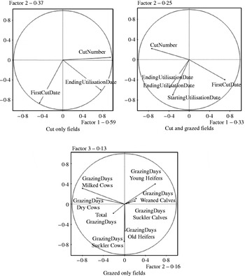
The results of the PCAs are described in Fig. 1 for the C, CG and G fields. Descriptions of the field use classes obtained with the mixed model analyses are summarized in Tables 4, 5 and 6.
Correlation circles in the two-dimensional space of the PCAs performed on the cut only fields (n=113), the cut and grazed fields (n=679) and the grazed only fields (n=794).

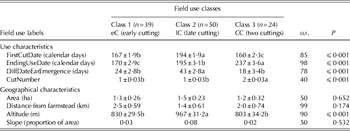
Use and geographical characteristics (least square means±s.e.m.) of the three field use classes identified for the cut only fields (C) (n=113)

Different letters within a row indicate significant differences at P<0·05.
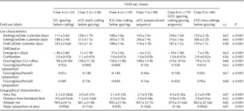
Use and geographical characteristics (least square means±s.e.m.) of the six field use classes identified for the cut and grazed fields (CG) (n=679)

Different letters within a row indicate significant differences at P<0·05.
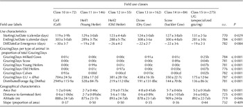
Use and geographical characteristics (least square means±s.e.m.) of the six field use classes identified for the grazed only fields (G) (n=794)

Different letters within a row indicate significant differences at P<0·05.
Cut only fields (C)
PCA on cut only fields (C, 113 fields) was performed with three active variables (the number of cuttings, the date of first cutting and the date corresponding to the end of field use) and explained 0·96 of the variability of the data with two factors (Fig. 1). The first factor is linked mainly to the number of cuttings and the second factor is characterized by the date of the first cutting and the date of the end of use. The hierarchical cluster analysis separated the population into three classes. Fields of Class 1 and Class 2 are only separated by the second factor (Fig. 1), while fields of Class 3 are separated from Classes 1 and 2 by the first factor.
Class 1 and Class 2 are characterized by one cutting whereas the fields of Class 3 are subjected to at least two cuttings (Table 4). Class 1 corresponds to fields cut once, early and Class 2 corresponds to fields cut once, late. The date of first cutting was significantly later in Class 2 than in Class 1. The fields of Class 3 are cut twice a year, with first cutting occurring early (significantly earlier than in Class 1). From these main uses, a label was attributed to each class as described in the last line of Table 4.
Cut and grazed fields (CG)
The PCA on cut and grazed fields (CG, 679 fields) was initially constructed on four variables related to cutting, i.e. the date of first cutting, the number of cuttings, the start and end dates for use. The final PCA explained 0·82 of the variability in the data using three factors. The first axis approximately relates to a scale involving date of first cutting (negative values) and the number of cuttings (positive values) (Fig. 1). The start and end dates for use both reflect the second axis, but are separated on axis 3 which is thus linked to the field use duration. The population was separated into six classes (Classes 4–9). Class 9 is distinct from the other classes along the first axis because it is the only class characterized by two cuttings. The fields of Class 4 are located at the top right corner of the PCA, being characterized by low values of start and end dates for use. Class 6 is positioned at the bottom of the plan, which corresponds to late use. Classes 7 and 8 are well separated along the third axis, and contrast in their difference in start and end dates for use.
Fields of Class 4 are subjected to early grazing in Period 1 (40 days before the theoretical date of the beginning of ear emergence) followed by one cutting (0·92 of the fields of Class 4 have this sequence of use) and their use ends early (Table 5). They represent the earliest start and end dates of use (only 77 days of use) and the highest proportion of grazing in Period 1. Fields of Classes 5 and 6 are characterized by one cut followed by grazing (0·88 and 0·99 of the fields characterized by this sequence of use were in classes 5 and 6, respectively). Grazing is mainly concentrated during period 4. Cutting occurs earlier in class 5 than in class 6 (11 days and 37 days after ear emergence), which results in a longer season of use in class 5 (+40 days of use). Class 7 brings together two types of sequences, each representing half of the population: cutting before grazing and grazing before cutting followed by grazing. First use corresponds to an early growth stage (6 days before ear emergence). Grazing occurs mainly in period 3. All the fields of Class 8 are characterized by a sequence of grazing before cutting followed by grazing, as demonstrated by (i) the difference between the date of first cutting and the starting date of use and (ii) by the distribution of grazing mainly between periods 1 and 4. This class shows the longest season of use (207 days between the average starting and ending use dates) and an early first use (39 days before ear emergence). The fields of Class 9 have a sequence with two cuttings followed by grazing (0·86 of the fields with this sequence of use). First cutting occurs early during the season (seven days after ear emergence) and grazing is concentrated in period 4. From these main uses, a label was attributed to each class as described in the last line of Table 5.
Grazed only fields
The PCA on grazed only fields (G, 794 fields) was initially constructed on nine variables related to grazing, i.e. the GrazingDays for all types of bovines except bulls (which accounted for only 0·02 of the fields), the total GrazingDays and the total amount of conserved forage distributed to the animals on the field during the grazing season. The final PCA explained 0·67 of the variability of the data using four factors. The first factor is linked solely to grazing by suckler and weaned calves. Figure 1 presents the results for the second and third factors, where the fields and classes were better spread out. The second factor, contrasted grazing by milked cows and Dcow with grazing by young heifers. The third factor is associated to grazing by Scow and old heifers. The hierarchical cluster analysis separated the population into six classes (Classes 10–15).
Fields of classes 10, 11, 12, 13 and 14 are mainly allocated to grazing by one type of animal (Table 6). The first grazing occurs very early for fields of all classes: 19–30 days before the date of ear emergence. Fields of class 10 are dedicated to grazing by suckler and weaned calves (0·93 of the GrazingDays on these fields, Table 6). They exhibit the earliest starting use date, the highest grazing intensity (704 LU×d/ha) and the highest amount of conserved forage distributed to the animals on the field (2949 kg DM/ha). Classes 11 and 12 correspond to fields grazed by young (0·99 of the GrazingDays) or old heifers (0·97), respectively. Class 11 fields have relatively low grazing intensity but with a high amount of distributed forage, whereas class 12 is grazed with medium intensity with a moderate amount of distributed forage (conserved forage distributed at grazing). Fields of class 13 are mainly grazed by milked cows (0·91 of the GrazingDays) with high intensity and are used longer in autumn than the other fields. Fields of class 14 are dedicated to grazing by Scow (0·89) with a moderate distribution of conserved forage. Class 15 is an unspecialized class, although these fields are used regularly by milked cows (0·25 of the GrazingDays). These fields exhibit the lowest use in terms of grazing intensity, grazing duration and distribution of conserved forage. From these main uses, a label was attributed to each class as described in the last line of Table 6.
Different geographical characteristics according to field use classes
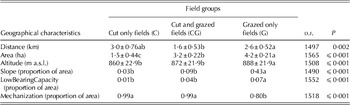
Relationships of the characteristics of the general categories of field use (C, CG and G fields) with the geographical characteristics obtained from the mixed model analysis are described in Table 7. Cut only fields are of small area, situated at a medium distance from the farmstead and at low altitude. They are well-adapted for mechanization as they are flat and have the best carrying capacity. Cut and grazed fields are on average close to the farmstead, well-adapted for mechanization and exhibit intermediate area and altitude. Grazed only fields are a long way from the farmstead, with a large area and relatively high altitude. They show a high proportion of area with slope and problems of carrying capacity, which results in low suitability for mechanization.
Geographical characteristics (least square means±s.e.m.) of the cut fields, cut and grazed fields and grazed only fields

Different letters within a row indicate significant differences at P<0·05.
However, these general trends conceal large intra-group variability. Consequently, relationships of the 15 classes of use with distance, area, altitude and slope obtained from mixed model analyses are presented in Tables 4–6.
The three classes of cut only fields do not present differences in terms of distance to farmstead, area or slope (Table 4). The early cutting and two cuttings classes that are cut earlier (calendar date) and at a younger growth stage (lower difference with theoretical date of ear emergence) than the late cutting class are also situated at a lower altitude.
In the cut and grazed field group, proportions of area with slope are low in all classes (see Table 5 for explanation of acronyms) even though they are higher in the GCG class than in the late cutting (lCG) class. The fields of classes with grazing and cutting sequences (GC and GCG) are larger and closer (Table 5) than fields of classes with cutting and grazing sequences (early cutting (eCG), lCG and CCG). The fields of the GC class are located at high altitude, which could explain why they are not grazed once more after cutting. The fields of the GCG class are close to the farmstead, which is consistent with two periods of grazing. As previously observed in the cut only field group, the eCG fields are situated at a lower altitude than the lCG fields.
The grazed only field classes are not different in terms of altitude and proportion of the area with slope (Table 6). The small fields close to the farmstead are grazed by calves when the large fields close to the farmstead are used by milked cows. The medium size fields far from the farmstead are grazed by old heifers, whereas the large fields far from the farmstead are used by Scow. The young heifers are located on small fields at an intermediate distance to the farmstead. The unspecialized grazed only fields have geographical characteristics similar to those dedicated to Scow, even though they tend to be closer and smaller.
Conceptual model of grassland use according to geographical determinants
Figure 2 proposes a conceptual model of grassland use according to grassland geographical characteristics. This figure relies on the significant differences between groups and classes that are presented in Tables 4–7. It highlights a hierarchy of geographical determinants of field uses. First of all, the slope and the bearing capacity could be related to the orientation between cut and grazed only fields. Secondly, the large area makes intensive use possible (cutting and grazing sequences or cow grazing), unlike smaller areas where use is less intense (cutting only or heifer grazing), possibly with a high quantity of distributed forage (grazing by calves). Finally, short distance is linked to use by animals that need to be close to the farmstead for milking (milked cows) and/or frequent forage distribution (calves). A low distance is also associated with early grazing of cut and grazed fields in order to facilitate herd management and movements until after turnout.
Discrimination tree of field uses according to geographical characteristics. The classes in bold correspond to the 15 field use classes constructed from the classification analysis. −slope+means that the arrow on the left side mentions the decision taken when the slope is low, and the arrow on the right side mentions the decision taken when the slope is high.

DISCUSSION
From the complexity observed in the surveyed farms, information has been extracted that characterizes the types of grassland uses observed in 1586 fields in traditional Salers systems and their links with geographical characteristics. These two issues of the present study are addressed in the first two sections of the discussion. Another aim of the study was to construct a conceptual model of grassland use that could be used in modelling approaches. The last section discusses how the model proposed in Fig. 2 could be utilized for modelling the interactions between forage productions and feeding requirements throughout the grazing season.
A fine characterization of field use in bovine grass-based systems
The classification approach presented here enabled 15 categories of grassland use to be distinguished throughout the grazing season. This classification, based on information on 1586 fields, is believed to be the most detailed to date; it highlights the diversity of cutting and grazing sequences on fields, with classes that account for the search for forage quality (eCG, CCG, GC) v. forage quantity (lCG) and classes that account for intensive use (GCG, CCG). Fleury et al. (Reference Fleury, Dubeuf and Jeanin1996) reported sequences comparable to those observed in CG or GCG fields in the present work. The ‘light grazing followed by cutting’ sequence is also mentioned in the work by Martin et al. (Reference Martin, Hossard, Theau, Therond, Josien, Cruz, Rellier, Martin-Clouaire and Duru2009) over a period corresponding to the first and second periods of use in the present study, which can thus be compared to the GC and GCG classes. For grazed only fields, Andrieu et al. (Reference Andrieu, Josien and Duru2007) previously identified fields intended for milked cows in opposition to fields for Dcow and heifers. The present study highlights a different classification, with a common class of fields for milked and Dcow and separated classes for young and old heifers grazing (Heif1 and Heif2). Grazed only fields were preferentially used by one type of animal (Calf, Heif1, Heif2, Dcow and Scow classes). This corresponds to the predetermined part of forage management. However, cut and grazed fields and unspecialized (uG) fields were used by several types of animals. It suggests that the grazing of these fields is not defined in advance, but decided during the season according to herd's needs. It constitutes a margin of flexibility that corresponds to the part of forage management adapted to the weather conditions.
The present classification was obtained from just one survey carried out in 2005, which may appear to be a limitation to the validity of the results. However, the farmers indicated that they used their fields in the usual manner in 2005 for 0·91 of the 1060 fields surveyed on this point. The uses observed can therefore be generalized for several years. The few adaptations mentioned generally concerned the elimination of the second cutting dictated by the drought conditions observed in the year of the survey (0·83 of cases). It therefore appears that adaptation to climatic uncertainties is more likely to occur at the level of harvests, and that practices are very stable on fields that are grazed only.
Geographical characteristics are strong drivers of grassland use
More than individual geographical constraints, there are combinations of constraints associated with each type of use. The present results reveal an overall hierarchy when taking constraints into account (indicated in the tree, Fig. 2) with first of all the slope, then the surface, the distance and finally the altitude.
The first criterion that conditions field use is its accessibility to mechanization related to its proportion of area with slope and its bearing capacity. Fields suitable for mechanization can be cut whereas the other fields can only be grazed. Slope has already been identified as a key factor for the occurrence of cutting (Andrieu et al. Reference Andrieu, Josien and Duru2007; Mottet et al. Reference Mottet, Ladet, Coqué and Gibon2006). Two related variables, accessibility for tractors and other machines, have been investigated by other authors (Thenail & Baudry Reference Thenail and Baudry2004; Mottet et al. Reference Mottet, Ladet, Coqué and Gibon2006).
The second determinant of use is the field area. In the case of fields that are grazed only, large fields have sufficient area to feed cows, milked or suckler. In the case of cut fields, the surface determines the possibility of grazing them equally. This slope/field surface hierarchy is consistent with that proposed by Martin et al. (Reference Martin, Hossard, Theau, Therond, Josien, Cruz, Rellier, Martin-Clouaire and Duru2009) in which accessibility to machinery determines the possibility of cutting, and ‘sufficient surface area to feed five animal units per hectare during 3 days at spring’ determines the possibility of grazing as a complement or not to cutting.
The third geographical determinant of uses is the distance from the cowshed. For grazed only fields, the nearby fields are allocated to calves and milked cows to minimize the walk to the milking parlour (Morlon & Benoit Reference Morlon and Benoit1990; Camacho Reference Camacho2004; Thenail & Baudry Reference Thenail and Baudry2004; Brunschwig et al. Reference Brunschwig, Josien and Bernhard2006; Andrieu et al. Reference Andrieu, Josien and Duru2007; Rapey et al. Reference Rapey, Gueringer, Gresset, Houdart, Josien and Bigot2008). Indeed, calves must be located close to the milked cows' fields, on pen fields where they are gathered twice a day (C. Bernhard, personal communication). For the cut and grazed fields, the distance (associated with the field area) determines the order and sequence of cutting and grazing: the fields grazed before cutting are larger and nearer than those that are cut first.
Altitude is the fourth determinant of the hierarchy. It influences the cutting date. It appears that the differences in altitude between early cutting (eC) and late cutting (lC) on the one hand and eCG and lCG on the other are too slight to modify the theoretical date of the start of ear emergence significantly. As a consequence, the present results suggest that the farmers cut the lowest fields as a priority and that cutting on the higher fields is held back until they can intervene, at an advanced stage of grass development (about 40 days after the start of ear emergence). This does not appear to be a very determining factor in the present study, but the work by Fleury et al. (Reference Fleury, Dubeuf and Jeanin1996) shows that altitude can influence the grazing of fields in alpine systems where the animals are up in the summer pastures for almost the whole of the grazing period. Andrieu et al. (Reference Andrieu, Josien and Duru2007) emphasized that fields grazed by heifers and Dcow are at a higher altitude than those grazed by the milked cows, but this element does not appear in the present results.
The model put forward in the present paper proposes a hierarchy of slope, area and distance to determine field use. This ranking is quite consistent with the one proposed by Martin et al. (Reference Martin, Hossard, Theau, Therond, Josien, Cruz, Rellier, Martin-Clouaire and Duru2009), where slope also has greater importance than area, being involved in the occurrence of cutting. However, Martin et al. (Reference Martin, Hossard, Theau, Therond, Josien, Cruz, Rellier, Martin-Clouaire and Duru2009) considered distance as being the first determinant of grassland use, distinguishing the fields grazed by dairy cows from those used in other ways. In the present context, suitability for mechanization, i.e. the slope, is the first determinant of grassland use, splitting between cut fields and grazed only fields. In Martin et al. (Reference Martin, Hossard, Theau, Therond, Josien, Cruz, Rellier, Martin-Clouaire and Duru2009), suitability for mechanization is also of great importance, acting in all the branches of their discrimination tree. Nevertheless, the area has a strong influence on grassland use in the present model, whereas it is only involved in the occurrence of grazing on isolated fields in Martin et al. (Reference Martin, Hossard, Theau, Therond, Josien, Cruz, Rellier, Martin-Clouaire and Duru2009). These variations could be associated with the different periods covered (spring vs. the whole grazing season) and to the different kinds of discrimination trees: the present work proposes a grassland use discrimination tree as opposed to a grassland use opportunities discrimination tree (Martin et al. Reference Martin, Hossard, Theau, Therond, Josien, Cruz, Rellier, Martin-Clouaire and Duru2009). Those authors constructed classes of field geographical constraints, which make several uses possible and which they associate with a potential flexibility of grassland use. In the present study, four pairs of classes (eC and CC, GC and GCG, eCG and CCG, Scow and uG) have no significant geographical difference. This result suggests that, within each pair of classes, the field uses would be interchangeable depending on the forage production conditions of the current year. The multiple uses of these fields could constitute flexibility for these systems.
From a typology to a conceptual model of grassland use in mountain bovine systems
The proposal presented in the current paper for a conceptual model (Fig. 2) seems valid for dairy and/or beef systems in mountain areas, insofar as it is based on the traditional Salers system, which combines the characteristics and practices of cutting and grazing of the two specialized systems.
Based on the conceptual model, probabilities of occurrence can be defined according to the geographical characteristics. Values are proposed based on the upper and/or lower limits of the confidence intervals of the average characteristics of the fields in each group (C, CG, G) or class of field use. Thus, the probability of cutting will be very high for fields with less than 0·15 of their surface area on a slope, and then will diminish to a very low level for fields with between 0·15 and 0·30 of sloping area. For grazed only fields, the probability of allocating a field to cows (milked or suckler) will increase rapidly in fields above an area of 3·5 ha. If situated at more than 1 km from the farmstead they will not generally be allocated to milked cows or calves, in agreement with the threshold identified by Brunschwig et al. (Reference Brunschwig, Josien and Bernhard2006) in a specialized dairy system.
The conceptual model can be incorporated into a whole farm model that simulates the interaction between the annual dynamics of forage production and animal requirements, predetermining field use allocation according to geographical characteristics, with a decision tree as in Sorel et al. (Reference Sorel, Viaud, Durand and Walter2010). Indeed, Jouven & Baumont (Reference Jouven and Baumont2008) discussed the geographical determinants of grassland use, grass production and biodiversity and concluded that they should be incorporated into their model, as it is initiated by Jacquot et al. (Reference Jacquot, Baumont and Brunschwig2009). As proposed by Berentsen et al. (Reference Berentsen, Giesen and Renkema2000), incorporation of geographical elements in a beef and/or dairy farm model would make it possible to simulate more realistic grass production and nitrogen balance.
Associated with a beef and/or dairy whole farm model, the discrimination tree would preferentially allocate some grazed-only fields to a single category of animals. For cut and grazed fields, the first use in spring would take place in accordance with their distance from the farmstead, cutting for the furthest away or early grazing followed by a cut for the nearest (C. Bernhard, personal communication). Later uses could be added according to the simulated evolution of grass growth and the needs of the herd.
The main conclusions from the present work are that geographical characteristics are some of the key determinants of grassland use. Grassland use in mountain bovine systems has been described, with 15 classes that account for the complexity of forage production and grazing management. Grassland use results from a hierarchy of geographical determinants. Slope and field area influence the allocation of a field to a specific use (cutting, grazing), distance from farmstead modifies both the type of use and the sequence of use (cutting before or after grazing) and then altitude influences the date of use. This constitutes a framework, formalized into the proposed model, which predetermines preferential field use allocation. This model enables simulations to be made of the spatio-temporal organization of forage management, relying on the dynamic interaction between animal requirements and grass growth, and depending on livestock management and weather conditions. With this structure, it will also be possible to consider the environmental performance, i.e. the positive and negative environmental impacts, at field and farm levels. Further investigation will study the influence of the field pattern level on this framework.
We thank Chantal Chassaing and Anne Farruggia for their helpful comments on the study and the manuscript, and Jane Curtis Williams for English revision. We acknowledge Hervé Laurent, Carine Desserre, the students of VetAgro Sup and the breeders of the ‘Tradition Salers’ association for their kind participation in the survey.