2 The inviscid mathematical model

Figure 1.

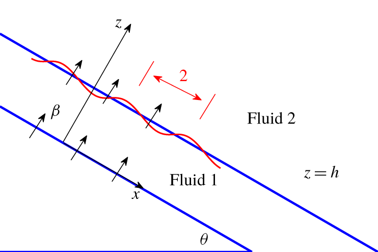
Schematic diagram of the flow configuration in dimensionless coordinates.

We consider the two-dimensional flow geometry depicted schematically in figure 1. The sloping side of the dug-out region is considered to be a flat plane that makes an angle $\unicode[STIX]{x1D703}$ to the horizontal, and the gravitational body force per mass acts vertically downward. We place a Cartesian coordinate system on the face of the cut-out wall as shown, with the $x$-axis running down the wall and the $z$-axis normal to it. We introduce unit vectors $\boldsymbol{e}_{\boldsymbol{x}}$ and $\boldsymbol{e}_{\boldsymbol{z}}$ pointing in the positive $x$- and $z$-directions, respectively. Since the acceleration of gravity $\boldsymbol{g}$ acts vertically downward, then the body force per mass experienced by the fluid is $\boldsymbol{g}=g(\sin \unicode[STIX]{x1D703}\boldsymbol{e}_{\boldsymbol{x}}-\cos \unicode[STIX]{x1D703}\boldsymbol{e}_{\boldsymbol{z}})$ in these coordinates. The scalar $g$ is the usual acceleration of gravity, and is a constant.

Fluid seeps through the rock and eventually leaches into the cut-out region through the sloping boundary at $z=0$. This pollutant fluid will be referred to here as fluid 1, and has density $\unicode[STIX]{x1D70C}_{1}$. It contains dissolved salts that have a molecular weight $\unicode[STIX]{x1D6FC}$ (mass per mole). This salty fluid 1 enters the region of fresh water, fluid 2, at a speed $W_{1}$ normal to the wall at $z=0$. The density of the fresh water in region 2 is $\unicode[STIX]{x1D70C}_{2}$. At the initial time $t=0$, we suppose that an interface is present between salty fluid 1 and fresh fluid 2, and is originally located on the plane $z=H$. The fresh and salty water are both assumed to be incompressible, and so as time progresses this interface advances into the fresh-water zone, so that its mean location is on the moving plane $z=H+W_{1}t$. The fresh water, too, is pushed normal to the wall $z=0$ at speed $W_{1}$ since it is incompressible. The two-dimensional fluid velocity vector is written $\boldsymbol{q}=u\boldsymbol{e}_{\boldsymbol{x}}+w\boldsymbol{e}_{\boldsymbol{z}}$ with tangential and normal components $u$ and $w$, and the location of the interface is represented as $z=\unicode[STIX]{x1D702}(x,t)$.

Fluid 2 is considered to be a sufficiently large reservoir of fresh rain water that it would remain idle except for the incoming salty fluid that pushes the interface between them. Its velocity components would therefore be $u_{2}=0$ and $w_{2}=W_{1}$. Lower fluid 1, however, is heavier than the fresh water above it, $\unicode[STIX]{x1D70C}_{1}>\unicode[STIX]{x1D70C}_{2}$ and so in addition to its movement normal to the sloping wall, it also moves down the wall with an acceleration proportional to the density difference between the two fluids. Thus its velocity vector components would be $u_{1}=gt\sin \unicode[STIX]{x1D703}(\unicode[STIX]{x1D70C}_{1}-\unicode[STIX]{x1D70C}_{2})/\unicode[STIX]{x1D70C}_{1}$ and $w_{1}=W_{1}$. We make the approximation that fluid 1 extends indefinitely far in both directions up and down the sloping wall, so that the location of the moving interface at $z=H+W_{1}t$ would not be significantly affected by the change in $u_{1}$ with time $t$. The salinity of lower fluid 1 is assumed to remain constant, and it therefore has the value $C_{1}=(\unicode[STIX]{x1D70C}_{1}-\unicode[STIX]{x1D70C}_{2})/\unicode[STIX]{x1D6FC}$ (moles per volume).

We introduce non-dimensional variables forthwith, by using some typical length scale $L$ in the $x$-direction as the reference for all lengths. Later, we will choose $L$ to be the half-wavelength of periodic K–H-type waves moving down the interface, so that a full wave occupies the interval $-1<x<1$ in these non-dimensional coordinates. The dimensionless wavelength is therefore $2$, as sketched in figure 1. Speeds are then scaled relative to the quantity $\sqrt{gL}$ and time is made dimensionless by reference to $\sqrt{L/g}$. The density $\unicode[STIX]{x1D70C}_{2}$ in the fresh water in fluid 2 is taken as the reference for density, so that pressures are made dimensionless relative to the quantity $\unicode[STIX]{x1D70C}_{2}gL$. The quantity $\unicode[STIX]{x1D70C}_{2}/\unicode[STIX]{x1D6FC}$ (moles per volume) is taken as the scale for concentration of salts in the fluid.

In these dimensionless variables, the inviscid equations are therefore dependent upon the three non-dimensional parameters

(2.1a-c)$$\begin{eqnarray}h=\frac{H}{L};\quad \unicode[STIX]{x1D6FD}=\frac{W_{1}}{\sqrt{gL}};\quad S_{1}=\frac{C_{1}\unicode[STIX]{x1D6FC}}{\unicode[STIX]{x1D70C}_{2}}=\frac{\unicode[STIX]{x1D70C}_{1}}{\unicode[STIX]{x1D70C}_{2}}-1.\end{eqnarray}$$

The first of these, $h$, is the dimensionless depth of the interface at the initial time $t=0$. The second parameter $\unicode[STIX]{x1D6FD}$ is a non-dimensional measure of the normal speed at the cut face, with which dense fluid 1 enters the region, and it may therefore be considered to be a Froude number based on entrance speed and half-wavelength. The final parameter $S_{1}$ is the dimensionless (constant) density anomaly in this lower fluid and thus serves as a proxy for the density difference between the lower and upper fluids, so that

(2.2)$$\begin{eqnarray}\unicode[STIX]{x1D70C}_{1}=\unicode[STIX]{x1D70C}_{2}(1+S_{1}).\end{eqnarray}$$

This is consistent with the model of Burns & Meiburg (Reference Burns and Meiburg2012), who also included the effect of particle transport (their equation (2.3)). Nevertheless, equation (2.2) is acknowledged to be a simple idealized representation of the density behaviour in real lakes, and particularly as no allowance is made here for temperature variations. Detailed experimental studies of the effects of temperature and electrical conductivity upon water density in several European lakes and reservoirs are discussed by Moreira et al. (Reference Moreira, Schultze, Rahn and Boehrer2016).

As each fluid is assumed to be inviscid in this section, there is no mechanism for the generation of vorticity, and so each fluid is assumed to flow irrotationally, with velocity potentials $\unicode[STIX]{x1D6F7}_{1}(x,z,t)$ and $\unicode[STIX]{x1D6F7}_{2}(x,z,t)$ in fluids 1 and 2, respectively. The fluid velocities in each fluid layer can then be written $\boldsymbol{q}_{1}=\unicode[STIX]{x1D735}\unicode[STIX]{x1D6F7}_{1}$ and $\boldsymbol{q}_{2}=\unicode[STIX]{x1D735}\unicode[STIX]{x1D6F7}_{2}$. Each fluid is incompressible, and so it follows that

(2.3)$$\begin{eqnarray}\displaystyle \left.\begin{array}{@{}c@{}}\unicode[STIX]{x1D6FB}^{2}\unicode[STIX]{x1D6F7}_{1}=0,\quad \text{in }0<z<\unicode[STIX]{x1D702}(x,t),\\ \unicode[STIX]{x1D6FB}^{2}\unicode[STIX]{x1D6F7}_{2}=0,\quad \text{in }z>\unicode[STIX]{x1D702}(x,t).\end{array}\right\} & & \displaystyle\end{eqnarray}$$

On the cut wall,

(2.4)$$\begin{eqnarray}w_{1}=\unicode[STIX]{x2202}\unicode[STIX]{x1D6F7}_{1}/\unicode[STIX]{x2202}z=\unicode[STIX]{x1D6FD}\quad \text{on }z=0.\end{eqnarray}$$

Since each fluid cannot cross its own interface, there are two kinematic equations that express this fact in each fluid. These can be written

(2.5)$$\begin{eqnarray}w_{k}=\frac{\unicode[STIX]{x2202}\unicode[STIX]{x1D702}}{\unicode[STIX]{x2202}t}+u_{k}\frac{\unicode[STIX]{x2202}\unicode[STIX]{x1D702}}{\unicode[STIX]{x2202}x},\quad k=1,2,\quad \text{on }z=\unicode[STIX]{x1D702}(x,t).\end{eqnarray}$$

Finally, there is also a dynamic condition to be imposed at the interface, expressing the fact that the pressures $p_{1}$ and $p_{2}$ must be equal on this boundary. In each fluid the pressure can be obtained from Bernoulli’s equation, so that the final non-dimensional form of this condition may be written

(2.6)$$\begin{eqnarray}\displaystyle & & \displaystyle \frac{\unicode[STIX]{x2202}\unicode[STIX]{x1D6F7}_{2}}{\unicode[STIX]{x2202}t}-(1+S_{1})\frac{\unicode[STIX]{x2202}\unicode[STIX]{x1D6F7}_{1}}{\unicode[STIX]{x2202}t}+\frac{1}{2}(u_{2}^{2}+w_{2}^{2})-\frac{1}{2}(1+S_{1})(u_{1}^{2}+w_{1}^{2})-S_{1}\unicode[STIX]{x1D702}\cos \unicode[STIX]{x1D703}\nonumber\\ \displaystyle & & \displaystyle \quad =-S_{1}x\sin \unicode[STIX]{x1D703}-S_{1}\cos \unicode[STIX]{x1D703}(h+\unicode[STIX]{x1D6FD}t)-\frac{1}{2}S_{1}\unicode[STIX]{x1D6FD}^{2}-\frac{t^{2}S_{1}^{2}\sin ^{2}\unicode[STIX]{x1D703}}{2(1+S_{1})}.\end{eqnarray}$$

We are interested in the formation of waves at the moving interface, and this fact now determines the meaning of the horizontal length scale $L$ used above to define dimensionless coordinates. It is here taken to be the half-wavelength of a disturbance at the interface, so that, in non-dimensional coordinates, the solution of interest is periodic in $x$, with a single wave lying on the interval $-1<x<1$.

This is a nonlinear free-boundary problem with period 2 in $x\in [-1,1]$, and we have formulated its solution using the ‘basic’ spectral method proposed by Forbes et al. (Reference Forbes, Chen and Trenham2007). Details are not presented further here, however, since it has been found that the interface develops a curvature singularity at early times, and the purely inviscid solution then ceases to exist for times later than this critical time. An advantage of the spectral method in Forbes et al. (Reference Forbes, Chen and Trenham2007) is that quantities such as curvature along the interface can be computed to very high accuracy, by exact differentiation of the series expressions for the interface shape, and the appearance of the curvature singularity can be seen clearly. This observation is consistent with the findings of Moore (Reference Moore1979), who presented an asymptotic analysis that demonstrated the formation of an interfacial curvature singularity within finite time, for the famous K–H shear instability. To overcome this rather severe limitation on the practical usefulness of our analysis, we will consider a Boussinesq model of the flow situation in § 4, in which there is a diffuse interfacial region rather than an infinitesimally thin region, as in the present inviscid model, and the density variation between the two fluid layers is required to be small. Nevertheless, there is value in analysing the linearized inviscid problem, and this is considered in the next section.

3 Linearized stability analysis

It is possible to derive linearized sets of equations for the inviscid problem discussed in § 2 by assuming a particular physical parameter is small, and of these, the most illuminating appears to consist of making a small-$\unicode[STIX]{x1D6FD}$ expansion about the base flow that has just a flat interface moving outwards. Accordingly, we expand the two velocity potentials $\unicode[STIX]{x1D6F7}_{1}$, $\unicode[STIX]{x1D6F7}_{2}$ and the interface elevation $\unicode[STIX]{x1D702}$ as

(3.1)$$\begin{eqnarray}\displaystyle \left.\begin{array}{@{}c@{}}\displaystyle \unicode[STIX]{x1D6F7}_{1}(x,z,t)=xt\sin \unicode[STIX]{x1D703}\frac{S_{1}}{(1+S_{1})}+\unicode[STIX]{x1D6FD}\unicode[STIX]{x1D6F7}_{11}(x,z,t)+O(\unicode[STIX]{x1D6FD}^{2})\\ \displaystyle \unicode[STIX]{x1D6F7}_{2}(x,z,t)=0+\unicode[STIX]{x1D6FD}\unicode[STIX]{x1D6F7}_{21}(x,z,t)+O(\unicode[STIX]{x1D6FD}^{2})\\ \displaystyle \unicode[STIX]{x1D702}(x,t)=h+\unicode[STIX]{x1D6FD}H_{1}(x,t)+O(\unicode[STIX]{x1D6FD}^{2}).\end{array}\right\} & & \displaystyle\end{eqnarray}$$

Clearly the two perturbation velocity potentials $\unicode[STIX]{x1D6F7}_{11}$ and $\unicode[STIX]{x1D6F7}_{21}$ still satisfy Laplace’s equations (2.3), although they now do so in the linearized fluid domains $0<z<h$ for fluid 1 and $z>h$ for fluid 2. The wall boundary condition (2.4) gives the requirement

(3.2)$$\begin{eqnarray}\frac{\unicode[STIX]{x2202}\unicode[STIX]{x1D6F7}_{11}}{\unicode[STIX]{x2202}z}=1\quad \text{on }z=0\end{eqnarray}$$

for the velocity potential in lower fluid 1.

The kinematic boundary condition on the interface, for lower fluid 1, is obtained from (2.5) by setting $k=1$. When linearized using the expansion (3.1) above, it gives

(3.3)$$\begin{eqnarray}\frac{\unicode[STIX]{x2202}\unicode[STIX]{x1D6F7}_{11}}{\unicode[STIX]{x2202}z}=\frac{\unicode[STIX]{x2202}H_{1}}{\unicode[STIX]{x2202}t}+t\sin \unicode[STIX]{x1D703}\frac{S_{1}}{(1+S_{1})}\frac{\unicode[STIX]{x2202}H_{1}}{\unicode[STIX]{x2202}x}\quad \text{on }z=h.\end{eqnarray}$$

Similarly, when expansion (3.1) is applied to the second kinematic condition in upper fluid 2 at the interface, obtained from (2.5) with $k=2$, it gives the requirement

(3.4)$$\begin{eqnarray}\frac{\unicode[STIX]{x2202}\unicode[STIX]{x1D6F7}_{21}}{\unicode[STIX]{x2202}z}=\frac{\unicode[STIX]{x2202}H_{1}}{\unicode[STIX]{x2202}t}\quad \text{on }z=h.\end{eqnarray}$$

Finally, the dynamical condition (2.6) is also linearized assuming small $\unicode[STIX]{x1D6FD}$ and the expansions (3.1) and yields the small-deviation approximate dynamical condition

(3.5)$$\begin{eqnarray}\frac{\unicode[STIX]{x2202}\unicode[STIX]{x1D6F7}_{21}}{\unicode[STIX]{x2202}t}-(1+S_{1})\frac{\unicode[STIX]{x2202}\unicode[STIX]{x1D6F7}_{11}}{\unicode[STIX]{x2202}t}-t\sin \unicode[STIX]{x1D703}S_{1}\frac{\unicode[STIX]{x2202}\unicode[STIX]{x1D6F7}_{11}}{\unicode[STIX]{x2202}x}-S_{1}\cos \unicode[STIX]{x1D703}H_{1}=-S_{1}t\cos \unicode[STIX]{x1D703}\quad \text{on }z=h.\end{eqnarray}$$

The linearized solution here is essentially just the first-mode term of a Fourier series, and so we take

(3.6)$$\begin{eqnarray}\displaystyle \left.\begin{array}{@{}c@{}}\unicode[STIX]{x1D6F7}_{11}(x,z,t)=z+[A(t)\cos (\unicode[STIX]{x03C0}x)+B(t)\sin (\unicode[STIX]{x03C0}x)]\cosh (\unicode[STIX]{x03C0}z)\\ \unicode[STIX]{x1D6F7}_{21}(x,z,t)=z+[C(t)\cos (\unicode[STIX]{x03C0}x)+D(t)\sin (\unicode[STIX]{x03C0}x)]\text{e}^{-\unicode[STIX]{x03C0}z},\end{array}\right\} & & \displaystyle\end{eqnarray}$$

and for the disturbance function for the interface profile,

(3.7)$$\begin{eqnarray}H_{1}(x,t)=t+P(t)\cos (\unicode[STIX]{x03C0}x)+Q(t)\sin (\unicode[STIX]{x03C0}x).\end{eqnarray}$$

These assumed solution forms already satisfy the condition (3.2) on the sloping surface. They are now substituted into the linearized boundary conditions (3.3)–(3.5) on the plane $z=h$, to determine the coefficients $A(t)$, $B(t)$, and so on.

The linearized kinematic condition (3.3) in fluid 1 gives the two requirements

(3.8)$$\begin{eqnarray}\displaystyle \left.\begin{array}{@{}c@{}}\displaystyle \unicode[STIX]{x03C0}\sinh (\unicode[STIX]{x03C0}h)A(t)=P^{\prime }(t)+\unicode[STIX]{x03C0}t\sin \unicode[STIX]{x1D703}\frac{S_{1}}{(1+S_{1})}Q(t)\\ \displaystyle \unicode[STIX]{x03C0}\sinh (\unicode[STIX]{x03C0}h)B(t)=Q^{\prime }(t)-\unicode[STIX]{x03C0}t\sin \unicode[STIX]{x1D703}\frac{S_{1}}{(1+S_{1})}P(t),\end{array}\right\} & & \displaystyle\end{eqnarray}$$

and the second linearized kinematic boundary condition (3.4) gives

(3.9)$$\begin{eqnarray}\displaystyle \left.\begin{array}{@{}c@{}}-\unicode[STIX]{x03C0}\text{e}^{-\unicode[STIX]{x03C0}h}C(t)=P^{\prime }(t)\\ -\unicode[STIX]{x03C0}\text{e}^{-\unicode[STIX]{x03C0}h}D(t)=Q^{\prime }(t).\end{array}\right\} & & \displaystyle\end{eqnarray}$$

Finally, the dynamic condition (3.5) yields

(3.10)$$\begin{eqnarray}\displaystyle \left.\begin{array}{@{}c@{}}\text{e}^{-\unicode[STIX]{x03C0}h}C^{\prime }(t)-(1+S_{1})\cosh (\unicode[STIX]{x03C0}h)A^{\prime }(t)-t\sin \unicode[STIX]{x1D703}S_{1}\unicode[STIX]{x03C0}\cosh (\unicode[STIX]{x03C0}h)B(t)-S_{1}\cos \unicode[STIX]{x1D703}P(t)=0\\ \text{e}^{-\unicode[STIX]{x03C0}h}D^{\prime }(t)-(1+S_{1})\cosh (\unicode[STIX]{x03C0}h)B^{\prime }(t)+t\sin \unicode[STIX]{x1D703}S_{1}\unicode[STIX]{x03C0}\cosh (\unicode[STIX]{x03C0}h)A(t)-S_{1}\cos \unicode[STIX]{x1D703}Q(t)=0.\end{array}\right\} & & \displaystyle \nonumber\\ \displaystyle & & \displaystyle\end{eqnarray}$$

These three sets of differential equations (3.8)–(3.10) are readily combined to create the system of two coupled second-order equations

(3.11)$$\begin{eqnarray}\displaystyle \left.\begin{array}{@{}c@{}}\displaystyle \unicode[STIX]{x1D705}P^{\prime \prime }(t)+2\unicode[STIX]{x1D706}tQ^{\prime }(t)+\unicode[STIX]{x1D706}Q(t)+\left(\unicode[STIX]{x1D707}-t^{2}\frac{\unicode[STIX]{x1D706}^{2}}{(1+S_{1})}\right)P(t)=0,\\ \displaystyle \unicode[STIX]{x1D705}Q^{\prime \prime }(t)-2\unicode[STIX]{x1D706}tP^{\prime }(t)-\unicode[STIX]{x1D706}P(t)+\left(\unicode[STIX]{x1D707}-t^{2}\frac{\unicode[STIX]{x1D706}^{2}}{(1+S_{1})}\right)Q(t)=0,\end{array}\right\} & & \displaystyle\end{eqnarray}$$

in which constants

(3.12)$$\begin{eqnarray}\displaystyle \left.\begin{array}{@{}c@{}}\unicode[STIX]{x1D705}=\tanh (\unicode[STIX]{x03C0}h)+(1+S_{1}),\\ \unicode[STIX]{x1D706}=\unicode[STIX]{x03C0}S_{1}\sin \unicode[STIX]{x1D703},\\ \unicode[STIX]{x1D707}=\unicode[STIX]{x03C0}S_{1}\cos \unicode[STIX]{x1D703}\tanh (\unicode[STIX]{x03C0}h)\end{array}\right\} & & \displaystyle\end{eqnarray}$$

have been defined for convenience. In effect, the two differential equations in (3.11) constitute a fourth-order system, from which it is too difficult to gain much useful information. This is because, while linear, these equations (3.11) do not have constant coefficients, and so no obvious solution technique presents itself.

In order to overcome this difficulty, we observe that, by defining the new complex variable

(3.13)$$\begin{eqnarray}R(t)=P(t)+\text{i}Q(t),\end{eqnarray}$$

the two equations in the system (3.11) can be written as the single second-order complex differential equation

(3.14)$$\begin{eqnarray}\unicode[STIX]{x1D705}R^{\prime \prime }(t)-2\text{i}\unicode[STIX]{x1D706}tR^{\prime }(t)-\text{i}\unicode[STIX]{x1D706}R(t)+\left(\unicode[STIX]{x1D707}-t^{2}\frac{\unicode[STIX]{x1D706}^{2}}{(1+S_{1})}\right)R(t)=0.\end{eqnarray}$$

This equation (3.14) can formally be solved in terms of Hermite and hypergeometric functions, but that is of little practical benefit here, and particularly as the nonlinear viscous results from § 2 show that the inviscid solution is approximately valid only for early times.

Consequently, an asymptotic solution to (3.14) is now sought, valid for early times. An appropriate small-$t$ approximation to (3.14) is simply the constant-coefficient equation

(3.15)$$\begin{eqnarray}\unicode[STIX]{x1D705}R^{\prime \prime }(t)+(\unicode[STIX]{x1D707}-\text{i}\unicode[STIX]{x1D706})R(t)\approx 0.\end{eqnarray}$$

This equation (3.16) has the general solution

(3.16)$$\begin{eqnarray}R(t)=C_{1}\text{e}^{\unicode[STIX]{x1D714}t}+C_{2}\text{e}^{-\unicode[STIX]{x1D714}t}\end{eqnarray}$$

in which $C_{1}$ and $C_{2}$ are complex constants and the complex number $\unicode[STIX]{x1D714}$ is obtained from the equation

(3.17)$$\begin{eqnarray}\unicode[STIX]{x1D714}^{2}=-(\unicode[STIX]{x1D707}-\text{i}\unicode[STIX]{x1D706})/\unicode[STIX]{x1D705}.\end{eqnarray}$$

We observe that the constant $\unicode[STIX]{x1D706}$ in (3.12) is always non-zero for every inclination angle $\unicode[STIX]{x1D703}>0$, and consequently, one of the two roots of equation (3.17) must always have positive real part. As a result, the solution (3.16) is always unstable. This is, perhaps, not surprising since for $\unicode[STIX]{x1D703}>0$ and positive relative density difference $S_{1}$ between the two fluids, the bottom fluid 1 will always be in motion relative to upper fluid 2, so that there is effectively a K–H-type flow present; the interface is known to be unstable for any relative motion between the two fluids there; see Drazin & Reid (Reference Drazin and Reid2004, p. 18). A similar instability was shown to occur also in cylindrical geometry between rotating inviscid fluids by Forbes & Cosgrove (Reference Forbes and Cosgrove2014).

4 Boussinesq viscous solution

Viscosity plays an important role in this problem, and we cope with viscous effects in this section using the Boussinesq approximation, in which the two-fluid system is regarded essentially as a single fluid with a variable density. Returning briefly to dimensional variables with $\unicode[STIX]{x1D70C}_{2}$ representing the density of the upper fresh fluid 2, then the density everywhere in this fluid is $\unicode[STIX]{x1D70C}=\unicode[STIX]{x1D70C}_{2}+\unicode[STIX]{x1D6FC}S$, where the dimensional constant $\unicode[STIX]{x1D6FC}$ represents the molecular weight of the dissolved salts in the fluid (mass per mole), as in § 2. 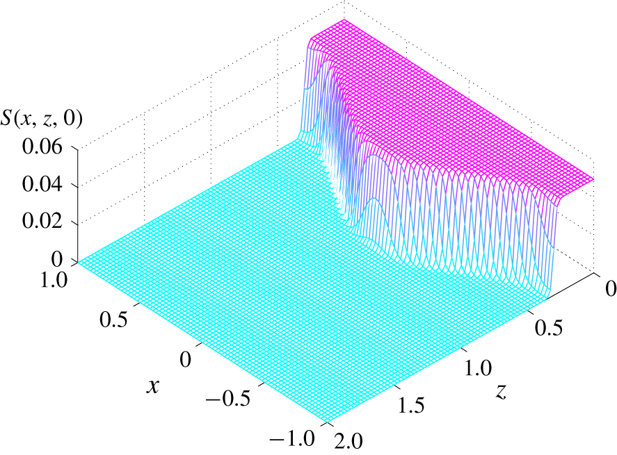Now the salinity concentration function $S(x,z,t)$ varies throughout the fluid, and at least initially, it is zero in the fresh fluid region 2 above the interface, and takes the value $C_{1}=(\unicode[STIX]{x1D70C}_{1}-\unicode[STIX]{x1D70C}_{2})/\unicode[STIX]{x1D6FC}$ (moles per volume) below the interface, with a smooth transition in salinity between these two values occurring in a narrow interfacial zone of finite width. A sketch of a typical initial saline profile is given in figure 2, and is discussed later in this section.

Figure 2.

The dimensionless initial density profile in (4.12). There is a smooth but rapid change across the interfacial zone $z=h+\unicode[STIX]{x1D716}\cos (\unicode[STIX]{x03C0}x)$, from fresh water above this contour to density $S_{1}$ below it. Here, $h=0.5$, $\unicode[STIX]{x1D716}=0.2$ and $S_{1}=0.05$.

Once again in the non-dimensional variables introduced in § 2, the fluid velocity vector $\boldsymbol{q}$ satisfies approximately the incompressibility condition

(4.1)$$\begin{eqnarray}\unicode[STIX]{x1D735}\boldsymbol{\cdot }\boldsymbol{q}=0,\end{eqnarray}$$

and the Navier–Stokes–Boussinesq equations

(4.2)$$\begin{eqnarray}\frac{\unicode[STIX]{x2202}\boldsymbol{q}}{\unicode[STIX]{x2202}t}+(\boldsymbol{q}\boldsymbol{\cdot }\unicode[STIX]{x1D735})\boldsymbol{q}+\unicode[STIX]{x1D735}p=(1+S)(\sin \unicode[STIX]{x1D703}\boldsymbol{e}_{\boldsymbol{x}}-\cos \unicode[STIX]{x1D703}\boldsymbol{e}_{\boldsymbol{z}})+\frac{1}{R_{e}}\unicode[STIX]{x1D6FB}^{2}\boldsymbol{q}\end{eqnarray}$$

that express the conservation of linear momentum approximately, for sufficiently small density perturbations in the fluid. The density concentration function $S(x,z,t)$ satisfies a transport equation

(4.3)$$\begin{eqnarray}\frac{\unicode[STIX]{x2202}S}{\unicode[STIX]{x2202}t}+(\boldsymbol{q}\boldsymbol{\cdot }\unicode[STIX]{x1D735})S=\unicode[STIX]{x1D70E}\unicode[STIX]{x1D6FB}^{2}S,\end{eqnarray}$$

in which a diffusion-type term has been added. The coefficient $\unicode[STIX]{x1D70E}$ is a constant related to the Prandtl number, as discussed by Farrow & Hocking (Reference Farrow and Hocking2006). Alternatively, the constant $1/\unicode[STIX]{x1D70E}$ may be regarded as a Schmidt number for the salinity (Burns & Meiburg Reference Burns and Meiburg2012, their equation (2.21)).

We follow Forbes (Reference Forbes2009) and satisfy the two-dimensional continuity equation identically, using a streamfunction $\unicode[STIX]{x1D6F9}(x,z,t)$. The velocity components $u$ and $w$ parallel and normal to the wall are expressed as

(4.4a,b)$$\begin{eqnarray}u=-\frac{\unicode[STIX]{x2202}\unicode[STIX]{x1D6F9}}{\unicode[STIX]{x2202}z};\quad w=\frac{\unicode[STIX]{x2202}\unicode[STIX]{x1D6F9}}{\unicode[STIX]{x2202}x}.\end{eqnarray}$$

In this planar flow, the vorticity vector $\unicode[STIX]{x1D73B}=\text{curl}\,\boldsymbol{q}$ has only one component $\unicode[STIX]{x1D701}(x,z,t)$, so that $\unicode[STIX]{x1D73B}=\unicode[STIX]{x1D701}\boldsymbol{e}_{\boldsymbol{y}}$ with

(4.5)$$\begin{eqnarray}\unicode[STIX]{x1D701}=\frac{\unicode[STIX]{x2202}u}{\unicode[STIX]{x2202}z}-\frac{\unicode[STIX]{x2202}w}{\unicode[STIX]{x2202}x}=-\unicode[STIX]{x1D6FB}^{2}\unicode[STIX]{x1D6F9},\end{eqnarray}$$

in view of equation (4.4) above. It is appropriate now to take the vector curl of the momentum equation (4.2). Since the vorticity vector only has the one component, this results in a scalar vorticity equation of the form

(4.6)$$\begin{eqnarray}\frac{\unicode[STIX]{x2202}\unicode[STIX]{x1D701}}{\unicode[STIX]{x2202}t}+(\boldsymbol{q}\boldsymbol{\cdot }\unicode[STIX]{x1D735})\unicode[STIX]{x1D701}=\unicode[STIX]{x1D735}S\boldsymbol{\cdot }(\cos \unicode[STIX]{x1D703}\boldsymbol{e}_{\boldsymbol{x}}+\sin \unicode[STIX]{x1D703}\boldsymbol{e}_{\boldsymbol{z}})+\frac{1}{R_{e}}\unicode[STIX]{x1D6FB}^{2}\unicode[STIX]{x1D701}.\end{eqnarray}$$

This equation shows immediately that vorticity is created by the gradient of density $S$ in the direction parallel to the wall, and diffused homogeneously by viscosity.

A semi-analytical solution is now sought to this system of equations (4.4)–(4.6), with the density equation (4.3), using a spectral approach. The streamfunction $\unicode[STIX]{x1D6F9}$ is taken to have the representation

(4.7)$$\begin{eqnarray}\displaystyle \unicode[STIX]{x1D6F9}(x,z,t) & = & \displaystyle \unicode[STIX]{x1D6FD}x+\mathop{\sum }_{n=1}^{N}B_{0n}(t)\left[\cos \left(\frac{n\unicode[STIX]{x03C0}z}{Z_{\infty }}\right)-1\right]\nonumber\\ \displaystyle & & \displaystyle +\,\mathop{\sum }_{m=1}^{M}\mathop{\sum }_{n=1}^{N}[-A_{mn}(t)\sin (m\unicode[STIX]{x03C0}x)+B_{mn}(t)\cos (m\unicode[STIX]{x03C0}x)]\left[\cos \left(\frac{n\unicode[STIX]{x03C0}z}{Z_{\infty }}\right)-1\right]\nonumber\\ \displaystyle & & \displaystyle\end{eqnarray}$$

and the density function is represented in a similar fashion by the series

(4.8)$$\begin{eqnarray}\displaystyle S(x,z,t) & = & \displaystyle S_{1}+\mathop{\sum }_{n=1}^{N}C_{0n}(t)\left[\cos \left(\frac{n\unicode[STIX]{x03C0}z}{Z_{\infty }}\right)-1\right]\nonumber\\ \displaystyle & & \displaystyle +\,\mathop{\sum }_{m=1}^{M}\mathop{\sum }_{n=1}^{N}[C_{mn}(t)\cos (m\unicode[STIX]{x03C0}x)+D_{mn}(t)\sin (m\unicode[STIX]{x03C0}x)]\left[\cos \left(\frac{n\unicode[STIX]{x03C0}z}{Z_{\infty }}\right)-1\right].\nonumber\\ \displaystyle & & \displaystyle\end{eqnarray}$$

In creating these expressions (4.7), (4.8), we have assumed a ‘computational window’ $-1<x<1$, $0<z<Z_{\infty }$, in which the constant $Z_{\infty }$ is taken to be sufficiently far away from the moving interface that its presence does not create any noticeable effects in the numerical solution to follow.

From equations (4.4), the two velocity components are now obtained at once from the series form (4.7), and they become

(4.9)$$\begin{eqnarray}\displaystyle u(x,z,t) & = & \displaystyle \mathop{\sum }_{n=1}^{N}B_{0n}(t)\left(\frac{n\unicode[STIX]{x03C0}}{Z_{\infty }}\right)\sin \left(\frac{n\unicode[STIX]{x03C0}z}{Z_{\infty }}\right)\nonumber\\ \displaystyle & & \displaystyle +\,\mathop{\sum }_{m=1}^{M}\mathop{\sum }_{n=1}^{N}[-A_{mn}(t)\sin (m\unicode[STIX]{x03C0}x)+B_{mn}(t)\cos (m\unicode[STIX]{x03C0}x)]\left(\frac{n\unicode[STIX]{x03C0}}{Z_{\infty }}\right)\sin \left(\frac{n\unicode[STIX]{x03C0}z}{Z_{\infty }}\right)\nonumber\\ \displaystyle w(x,z,t) & = & \displaystyle \unicode[STIX]{x1D6FD}-\mathop{\sum }_{m=1}^{M}\mathop{\sum }_{n=1}^{N}[A_{mn}(t)\cos (m\unicode[STIX]{x03C0}x)+B_{mn}(t)\sin (m\unicode[STIX]{x03C0}x)](m\unicode[STIX]{x03C0})\left[\cos \left(\frac{n\unicode[STIX]{x03C0}z}{Z_{\infty }}\right)-1\right].\nonumber\\ \displaystyle & & \displaystyle\end{eqnarray}$$

From (4.9), the boundary conditions on the sloping wall $z=0$ are easily seen to be $u=0$ and $w=\unicode[STIX]{x1D6FD}$. This has been chosen to be consistent with the inviscid boundary condition (2.4), but also adds a no-slip condition at the wall, appropriate now to the inclusion of fluid viscosity in the model. Consequently, a viscous boundary layer is expected near the sloping wall at $x=0$. However, at the edge of the computational window, $z=Z_{\infty }$, while the normal speed component is again required to have the value $w=\unicode[STIX]{x1D6FD}$, there is no such restriction on the component $u$ parallel to the wall.

The vorticity is likewise obtained at once from these expressions, using (4.5). This gives

(4.10)$$\begin{eqnarray}\displaystyle & & \displaystyle \unicode[STIX]{x1D701}(x,z,t)=\mathop{\sum }_{n=1}^{N}B_{0n}(t)\left(\frac{n\unicode[STIX]{x03C0}}{Z_{\infty }}\right)^{2}\cos \left(\frac{n\unicode[STIX]{x03C0}z}{Z_{\infty }}\right)\nonumber\\ \displaystyle & & \displaystyle \quad +\,\mathop{\sum }_{m=1}^{M}\mathop{\sum }_{n=1}^{N}[-A_{mn}(t)\sin (m\unicode[STIX]{x03C0}x)+B_{mn}(t)\cos (m\unicode[STIX]{x03C0}x)]\left[K_{mn}^{2}\cos \left(\frac{n\unicode[STIX]{x03C0}z}{Z_{\infty }}\right)-(m\unicode[STIX]{x03C0})^{2}\right].\nonumber\\ \displaystyle & & \displaystyle\end{eqnarray}$$

In this expression, we have introduced the constants

(4.11)$$\begin{eqnarray}K_{mn}^{2}=(m\unicode[STIX]{x03C0})^{2}+(n\unicode[STIX]{x03C0}/Z_{\infty })^{2}\end{eqnarray}$$

for convenience. This expression (4.10) for the vorticity, along with the series representation (4.8), are now substituted into the scalar vorticity equation (4.6). The resulting expression is extremely lengthy, but is next subject to Fourier analysis. First, it is multiplied by basis functions $\cos (\ell \unicode[STIX]{x03C0}z/Z_{\infty })$, $\ell =1,2,\ldots ,N$ and integrated over the fluid domain $-1<x<1$, $0<z<Z_{\infty }$. A system of $N$ equations for the differentiated Fourier coefficients $B_{0\ell }^{\prime }(t)$ is thus obtained, and is given in appendix A as equation (A 1). Next, the vorticity equation is multiplied by the even-mode basis functions $\cos (k\unicode[STIX]{x03C0}x)\cos (\ell \unicode[STIX]{x03C0}z/Z_{\infty })$ and integrated again over the fluid domain, to yield a system of equations for the differentiated coefficients $B_{k\ell }^{\prime }(t)$, $k=1,2,\ldots ,M$, $\ell =1,2,\ldots ,N$. These are given by the expressions (A 2) in appendix A. Finally, the vorticity equation is multiplied by the odd-mode basis functions $\sin (k\unicode[STIX]{x03C0}x)\cos (\ell \unicode[STIX]{x03C0}z/Z_{\infty })$ and again integrated, this time to produce equations (A 3) for the coefficients $A_{k\ell }^{\prime }(t)$.

The density transport equation (4.3) is similarly analysed. To begin, it is multiplied by basis functions $\cos (\ell \unicode[STIX]{x03C0}z/Z_{\infty })$, $\ell =1,2,\ldots ,N$ and integrated over the fluid domain $-1<x<1$, $0<z<Z_{\infty }$. This yields a system of equations for the differentiated Fourier coefficients $C_{0\ell }^{\prime }(t)$, and these, too, are given in full in appendix A as equations (A 6). The even and odd Fourier-mode components in this equation are then extracted, multiplying first by $\cos (k\unicode[STIX]{x03C0}x)\cos (\ell \unicode[STIX]{x03C0}z/Z_{\infty })$ and then by $\sin (k\unicode[STIX]{x03C0}x)\cos (\ell \unicode[STIX]{x03C0}z/Z_{\infty })$ and integrating over the fluid domain, as for the vorticity equation above. These each give a further system of equations, first for $C_{k\ell }^{\prime }(t)$ and then for $D_{k\ell }^{\prime }(t)$, $k=1,2,\ldots ,M$, $\ell =1,2,\ldots ,N$. These are given by expressions (A 7) and (A 8) in appendix A.

The resulting system of equations (A 1)–(A 8) in appendix A consists of a total of $4MN+2N$ ordinary differential equations for the Fourier coefficients in the series representations (4.7), (4.8) of the flow variables and the density concentration. These are integrated forward in time, using the classical fourth-order explicit Runge–Kutta method (Atkinson Reference Atkinson1978, p. 371). The integrals that appear in some terms in equations (A 1)–(A 8) were evaluated to very high accuracy using Gauss–Legendre quadrature with a large number of mesh points. For this, we have again used the routine lgwt written by von Winckel (Reference von Winckel2004). This large system of equations was solved in parallel using suitable parallelizing hardware and software, as discussed in Walters & Forbes (Reference Walters and Forbes2019). Using this computer architecture, we are able to use $M=144,N=288$ coefficients, with $720\times 1440$ mesh points, so generating results of great accuracy. A full solution up to $t=30$ using 400 time steps per (dimensionless) unit of time, can typically be generated in approximately 55 hours.

The numerical scheme described here is based on the methods developed by Walters & Forbes (Reference Walters and Forbes2019) for two-dimensional and three-dimensional unsteady interfacial flows in Boussinesq fluids. They describe in detail their use of a bi-streamfunction approach and the computer hardware they developed for these computations, and they give several examples of the use of these techniques in different applications. Nevertheless, a spectral approach to the computation of flows in density-stratified, rotating fluids is also presented by Winters, MacKinnon & Mills (Reference Winters, MacKinnon and Mills2004), and it, too, makes the Boussinesq approximation. The method of Walters & Forbes (Reference Walters and Forbes2019) differs from this, in that it eliminates the pressure variable using a vorticity equation (like (4.6) in planar flow) and solves only for density and one streamfunction $\unicode[STIX]{x1D6F9}$ (in two dimensions) or two streamfunctions $\unicode[STIX]{x1D6F9}$ and $\unicode[STIX]{x1D712}$ (in three-dimensional flow). By contrast, Winters et al. (Reference Winters, MacKinnon and Mills2004) retain primitive variables in their formulation, and express each velocity component and pressure as Fourier series in space, with time-dependent coefficients. They likewise derive differential equations for their Fourier coefficients, which they integrate forward in time, using a third-order Adams–Bashforth method, rather than the fourth-order Runge–Kutta method used here. In addition, they treat the diffusion terms in the Fourier space exactly, using an integrating factor; this was avoided here to circumvent any possibility of numerical ill conditioning.

It is necessary, here, to comment on the choice of initial conditions for this problem. At time $t=0$, we assume that the flow is purely normal to the sloping plane, due solely to the inflow of denser water at the cut face. Thus $w(x,z,0)=\unicode[STIX]{x1D6FD}$ and so the coefficients in the series terms in (4.7) are simply set to zero: $A_{mn}(0)=0$, $B_{mn}(0)=0$. Far below the interface, the density of the fluid becomes constant with the value $S_{1}$, but above is fresh water for which $S=0$. For definiteness, the interface is assumed to have a simple cosine shape at $t=0$, and it is required that the density should vary rapidly but smoothly across this zone. Accordingly, we set

(4.12)$$\begin{eqnarray}S(x,z,0)=\frac{S_{1}}{1+\exp [\unicode[STIX]{x1D706}_{S}(z-h-\unicode[STIX]{x1D716}\cos (\unicode[STIX]{x03C0}x))]}.\end{eqnarray}$$

The constant $\unicode[STIX]{x1D706}_{S}$ is chosen to determine the width of the initial interfacial zone, and we choose $\unicode[STIX]{x1D706}_{S}=100$. A sketch of this initial density function is given in figure 2, in which $h=0.5$ and $\unicode[STIX]{x1D716}=0.2$, and for illustrative purposes the normal coordinate is shown over the interval $0<z<2$. The density parameter is chosen to be $S_{1}=0.05$.

It follows from Fourier analysis of the spectral form (4.8) that the initial values of the coefficients in that expression are given by

(4.13)$$\begin{eqnarray}C_{0\ell }(0)=\frac{1}{Z_{\infty }}\int _{-1}^{1}\int _{0}^{Z_{\infty }}S(x,z,0)\cos \left(\frac{\ell \unicode[STIX]{x03C0}z}{Z_{\infty }}\right)\,\text{d}z\,\text{d}x,\quad \ell =1,2,\ldots ,N\end{eqnarray}$$

for the zeroth Fourier modes in $x$, and for higher even modes,

(4.14)$$\begin{eqnarray}\displaystyle C_{k\ell }(0) & = & \displaystyle \frac{2}{Z_{\infty }}\int _{-1}^{1}\int _{0}^{Z_{\infty }}S(x,z,0)\cos (k\unicode[STIX]{x03C0}x)\cos \left(\frac{\ell \unicode[STIX]{x03C0}z}{Z_{\infty }}\right)\,\text{d}z\,\text{d}x,\nonumber\\ \displaystyle & & \displaystyle k=1,2,\ldots ,M\quad \ell =1,2,\ldots ,N.\end{eqnarray}$$

The higher odd-mode coefficients $D_{k\ell }(0)$ are similar, except that the functions $\cos (k\unicode[STIX]{x03C0}x)$ are replaced with $\sin (k\unicode[STIX]{x03C0}x)$ in (4.14).

If the initial condition (4.12) is approximated by one in which there is an abrupt jump from $S=0$ to $S=S_{1}$, at an interface of zero width, then the integrals (4.13) and (4.14) can be evaluated in closed form, using an identity from Gradshteyn & Ryzhik (Reference Gradshteyn and Ryzhik2000, formula 3.715.13). Because (4.12) is even in $x$, the odd-mode coefficients are all zero, so that $D_{k\ell }(0)=0$. Then after some algebra, we obtain

(4.15)$$\begin{eqnarray}\displaystyle \left.\begin{array}{@{}c@{}}\displaystyle C_{0\ell }(0)=\frac{2S_{1}}{\ell \unicode[STIX]{x03C0}}\sin \left(\frac{\ell \unicode[STIX]{x03C0}h}{Z_{\infty }}\right)\text{J}_{0}\left(\frac{\ell \unicode[STIX]{x03C0}\unicode[STIX]{x1D716}}{Z_{\infty }}\right),\\ \displaystyle C_{k\ell }(0)=\frac{4S_{1}}{\ell \unicode[STIX]{x03C0}}\sin \left(\frac{\ell \unicode[STIX]{x03C0}h}{Z_{\infty }}+\frac{k\unicode[STIX]{x03C0}}{2}\right)\text{J}_{k}\left(\frac{\ell \unicode[STIX]{x03C0}\unicode[STIX]{x1D716}}{Z_{\infty }}\right),\end{array}\right\} & & \displaystyle\end{eqnarray}$$

in which the symbol $\text{J}_{k}(z)$ denotes the first-kind Bessel function of order $k$. In practice, the use of the coefficients (4.15) in the series (4.8) recreates the initial density profile (4.12) faithfully, except for the presence of small ripples near the location of the interface $z\approx h+\unicode[STIX]{x1D716}\cos (\unicode[STIX]{x03C0}x)$. It is well known that a discontinuous profile has a Fourier representation that contains small-amplitude oscillations, as a result of the Gibbs phenomenon (see Kreyszig (Reference Kreyszig2011, p. 515)). We have employed smoothing techniques, such as Lanczos smoothing, to eliminate these oscillations and this serves as a useful check on the accuracy of our computed initial coefficients when using (4.13), (4.14) purely numerically.

5 Linearized Boussinesq theory

In the Boussinesq theory of the preceding § 4, the interface is represented as a narrow zone in which density changes smoothly but rapidly. In addition, this theory requires that the changes in density across the fluid region are small everywhere. Equivalently, the density function $S(x,z,t)$, which is zero in the fresh water and of typical order $S_{1}$ in the denser part, must remain small, since it follows from (2.1) that $S_{1}=(\unicode[STIX]{x1D70C}_{1}-\unicode[STIX]{x1D70C}_{2})/\unicode[STIX]{x1D70C}_{2}$. Thus a linearization, in which $S_{1}$ is taken to be the small parameter, is entirely consistent with Boussinesq theory, and is the topic of this present section.

We assume the flow variables may be expressed by means of the expansion

(5.1)$$\begin{eqnarray}\displaystyle \left.\begin{array}{@{}c@{}}\unicode[STIX]{x1D6F9}(x,z,t)=\unicode[STIX]{x1D6FD}x+S_{1}\unicode[STIX]{x1D6F9}^{L}(x,z,t)+O(S_{1}^{2}),\\ u(x,z,t)=0+S_{1}u^{L}(x,z,t)+O(S_{1}^{2}),\\ w(x,z,t)=\unicode[STIX]{x1D6FD}+S_{1}w^{L}(x,z,t)+O(S_{1}^{2}),\\ \unicode[STIX]{x1D701}(x,t)=0+S_{1}\unicode[STIX]{x1D701}^{L}(x,t)+O(S_{1}^{2}),\\ S(x,z,t)=0+S_{1}S^{L}(x,z,t)+O(S_{1}^{2}).\end{array}\right\} & & \displaystyle\end{eqnarray}$$

The linearized contributions $u^{L}$ and $w^{L}$ to the flow speeds in the $x$- and $z$-directions are related to the linearized streamfunction $\unicode[STIX]{x1D6F9}^{L}$ by the same equations (4.4) as previously. The linearized vorticity function $\unicode[STIX]{x1D701}^{L}$ is likewise related to the linearized velocity components and streamfunction by the same equation (4.5) as before.

As a consequence of the expansions (5.1), the density transport equation (4.3) linearizes to

(5.2)$$\begin{eqnarray}\frac{\unicode[STIX]{x2202}S^{L}}{\unicode[STIX]{x2202}t}+\unicode[STIX]{x1D6FD}\frac{\unicode[STIX]{x2202}S^{L}}{\unicode[STIX]{x2202}z}=\unicode[STIX]{x1D70E}\unicode[STIX]{x1D6FB}^{2}S^{L},\end{eqnarray}$$

and the vorticity equation (4.6) takes the linearized form

(5.3)$$\begin{eqnarray}\frac{\unicode[STIX]{x2202}\unicode[STIX]{x1D701}^{L}}{\unicode[STIX]{x2202}t}+\unicode[STIX]{x1D6FD}\frac{\unicode[STIX]{x2202}\unicode[STIX]{x1D701}^{L}}{\unicode[STIX]{x2202}z}=\cos \unicode[STIX]{x1D703}\frac{\unicode[STIX]{x2202}S^{L}}{\unicode[STIX]{x2202}x}+\sin \unicode[STIX]{x1D703}\frac{\unicode[STIX]{x2202}S^{L}}{\unicode[STIX]{x2202}z}+\frac{1}{R_{e}}\unicode[STIX]{x1D6FB}^{2}\unicode[STIX]{x1D701}^{L}.\end{eqnarray}$$

The boundary conditions are

(5.4a-c)$$\begin{eqnarray}u^{L}\rightarrow 0,\quad w^{L}\rightarrow 0,\quad S^{L}\rightarrow 0\quad \text{as }z\rightarrow \infty\end{eqnarray}$$

far away, and

(5.5a-c)$$\begin{eqnarray}u^{L}=0,\quad w^{L}=0,\quad S^{L}=1\quad \text{on }z=0,\end{eqnarray}$$

at the quarry wall $z=0$ itself. We ignore boundary-layer effects at the wall, particularly as there is fluid seepage motion through that plane, and so take

(5.6)$$\begin{eqnarray}\unicode[STIX]{x1D701}^{L}=0\quad \text{at }z=0.\end{eqnarray}$$

Finally, there is a requirement to specify initial conditions. As in § 4, it is assumed that the initial flow is purely due to the seepage of dense fluid at the plane $z=0$. Thus $u=0$ and $w=\unicode[STIX]{x1D6FD}$ throughout, and from the expansion (5.1) it follows that

(5.7a-c)$$\begin{eqnarray}u^{L}=0,\quad w^{L}=0,\quad \unicode[STIX]{x1D701}^{L}=0\quad \text{at }t=0.\end{eqnarray}$$

It will also be necessary to specify an initial density $S^{L}(x,z,0)$ in the linearized problem, and this will be considered shortly.

It is at once obvious that the linearized density $S^{L}(x,z,t)$ can be considered separately, since equation (5.2) shows that it de-couples from the other variables. It becomes evident, too, that the only way in which this equation can be solved sensibly, subject to the boundary condition (5.5) that requires $S^{L}=1$ at $z=0$ for all times $t$, is for there to be a moving front $z=\unicode[STIX]{x1D6FD}t$, behind which $S^{L}=1$ and ahead of which the linearized density function $S^{L}$ is free to decay. To enforce this, it is convenient to introduce a moving coordinate system with a new variable

(5.8)$$\begin{eqnarray}\unicode[STIX]{x1D709}=z-\unicode[STIX]{x1D6FD}t,\end{eqnarray}$$

and use the chain rule of calculus to regard the function $S^{L}(x,z,t)$ ahead of the moving front $\unicode[STIX]{x1D709}=0$ as having the representation $S^{L}(x,\unicode[STIX]{x1D709}(z,t),t)$ in this new coordinate (5.8). We therefore choose to represent the linearized density function in the form

(5.9)$$\begin{eqnarray}S^{L}(x,z,t)=\left\{\begin{array}{@{}ll@{}}1, & 0<z<\unicode[STIX]{x1D6FD}t\\ \text{e}^{-\unicode[STIX]{x1D6FC}_{1}\unicode[STIX]{x1D709}}+R^{L}(x,\unicode[STIX]{x1D709},t), & 0<\unicode[STIX]{x1D709}<\infty .\end{array}\right.\end{eqnarray}$$

Here, the constant $\unicode[STIX]{x1D6FC}_{1}>0$ may be determined later.

As a consequence of this choice (5.9), the new function $R^{L}(x,\unicode[STIX]{x1D709},t)$ now satisfies the inhomogeneous partial differential equation

(5.10)$$\begin{eqnarray}\frac{\unicode[STIX]{x2202}R^{L}}{\unicode[STIX]{x2202}t}=\unicode[STIX]{x1D70E}\biggl(\frac{\unicode[STIX]{x2202}^{2}R^{L}}{\unicode[STIX]{x2202}x^{2}}+\frac{\unicode[STIX]{x2202}^{2}R^{L}}{\unicode[STIX]{x2202}\unicode[STIX]{x1D709}^{2}}\biggr)+\unicode[STIX]{x1D70E}\unicode[STIX]{x1D6FC}^{2}\text{e}^{-\unicode[STIX]{x1D6FC}_{1}\unicode[STIX]{x1D709}}\end{eqnarray}$$

ahead of the moving front, in $0<\unicode[STIX]{x1D709}<\infty$. On the front itself,

(5.11)$$\begin{eqnarray}R^{L}=0\quad \text{on }\unicode[STIX]{x1D709}=0,\end{eqnarray}$$

and

(5.12)$$\begin{eqnarray}R^{L}\rightarrow 0\quad \text{as }\unicode[STIX]{x1D709}\rightarrow \infty .\end{eqnarray}$$

We also require periodic boundary conditions, so that $R^{L}$ and its derivatives are equal at $x=-1$ and $x=1$.

Since this new function $R^{L}$ now satisfies the homogeneous boundary condition (5.11) at the moving front $\unicode[STIX]{x1D709}=0$, it is appropriate to introduce the Fourier sine transform

(5.13)$$\begin{eqnarray}\widetilde{R}(x,t;k)=\sqrt{\frac{2}{\unicode[STIX]{x03C0}}}\int _{0}^{\infty }R^{L}(x,\unicode[STIX]{x1D709},t)\sin (k\unicode[STIX]{x1D709})\,\text{d}\unicode[STIX]{x1D709}\end{eqnarray}$$

and its inverse

(5.14)$$\begin{eqnarray}R^{L}(x,\unicode[STIX]{x1D709},t)=\sqrt{\frac{2}{\unicode[STIX]{x03C0}}}\int _{0}^{\infty }\widetilde{R}(x,t;k)\sin (k\unicode[STIX]{x1D709})\,\text{d}k.\end{eqnarray}$$

The Fourier transform (5.13) applied to equation (5.10) results in

(5.15)$$\begin{eqnarray}\frac{\unicode[STIX]{x2202}\widetilde{R}}{\unicode[STIX]{x2202}t}=\unicode[STIX]{x1D70E}\frac{\unicode[STIX]{x2202}^{2}\widetilde{R}}{\unicode[STIX]{x2202}x^{2}}-\unicode[STIX]{x1D70E}k^{2}\widetilde{R}+\unicode[STIX]{x1D70E}\unicode[STIX]{x1D6FC}_{1}^{2}\sqrt{\frac{2}{\unicode[STIX]{x03C0}}}\frac{k}{\unicode[STIX]{x1D6FC}_{1}^{2}+k^{2}}.\end{eqnarray}$$

Since a solution is required having period 2 in $x$, separation of variables now yields the solution for the Fourier transform (5.13) in the form

(5.16)$$\begin{eqnarray}\displaystyle \widetilde{R}(x,t;k) & = & \displaystyle \sqrt{\frac{2}{\unicode[STIX]{x03C0}}}\frac{\unicode[STIX]{x1D6FC}_{1}^{2}}{k(\unicode[STIX]{x1D6FC}_{1}^{2}+k^{2})}+C_{0}(k)\exp (-\unicode[STIX]{x1D70E}k^{2}t)\nonumber\\ \displaystyle & & \displaystyle +\,\mathop{\sum }_{n=1}^{\infty }[C_{n}(k)\cos (n\unicode[STIX]{x03C0}x)+D_{n}(k)\sin (n\unicode[STIX]{x03C0}x)]\exp [-\unicode[STIX]{x1D70E}t(n^{2}\unicode[STIX]{x03C0}^{2}+k^{2})].\end{eqnarray}$$

The Fourier coefficients $C_{n}$ and $D_{n}$ are determined by the choice of initial condition.

To be consistent with the initial condition (4.12) discussed in § 4, the function $R^{L}$ defined in (5.9) is chosen to have the initial profile

(5.17)$$\begin{eqnarray}R^{L}(x,\unicode[STIX]{x1D709},0)=\left\{\begin{array}{@{}ll@{}}-\exp (-\unicode[STIX]{x1D6FC}_{1}\unicode[STIX]{x1D709}), & h+\unicode[STIX]{x1D716}\cos (\unicode[STIX]{x03C0}x)<\unicode[STIX]{x1D709}<\infty \\ 1-\exp (-\unicode[STIX]{x1D6FC}_{1}\unicode[STIX]{x1D709}), & 0<\unicode[STIX]{x1D709}<h+\unicode[STIX]{x1D716}\cos (\unicode[STIX]{x03C0}x)\end{array}\right.\end{eqnarray}$$

ahead of the moving front. The Fourier transform (5.13) of this initial condition (5.17) gives the initial condition in frequency space to be

(5.18)$$\begin{eqnarray}\widetilde{R}(x,0;k)=\sqrt{\frac{2}{\unicode[STIX]{x03C0}}}\frac{1}{k}\left[-\cos (kh+k\unicode[STIX]{x1D716}\cos (\unicode[STIX]{x03C0}x))+\frac{\unicode[STIX]{x1D6FC}_{1}^{2}}{\unicode[STIX]{x1D6FC}_{1}^{2}+k^{2}}\right],\end{eqnarray}$$

and this must be made equal to the expression (5.16) evaluated at $t=0$. Analysis of the Fourier series in $x$ then shows the Fourier coefficients to be

(5.19)$$\begin{eqnarray}\displaystyle \left.\begin{array}{@{}c@{}}\displaystyle C_{0}(k)=-\sqrt{\frac{2}{\unicode[STIX]{x03C0}}}\frac{1}{2k}\int _{-1}^{1}\cos (kh+k\unicode[STIX]{x1D716}\cos (\unicode[STIX]{x03C0}x))\,\text{d}x,\\ \displaystyle C_{n}(k)=-\sqrt{\frac{2}{\unicode[STIX]{x03C0}}}\frac{1}{k}\int _{-1}^{1}\cos (kh+k\unicode[STIX]{x1D716}\cos (\unicode[STIX]{x03C0}x))\cos (n\unicode[STIX]{x03C0}x)\,\text{d}x,\\ \displaystyle D_{n}(k)=-\sqrt{\frac{2}{\unicode[STIX]{x03C0}}}\frac{1}{k}\int _{-1}^{1}\cos (kh+k\unicode[STIX]{x1D716}\cos (\unicode[STIX]{x03C0}x))\sin (n\unicode[STIX]{x03C0}x)\,\text{d}x.\end{array}\right\} & & \displaystyle\end{eqnarray}$$

Since the initial density profile (5.17) is symmetric in $x$, it follows that the coefficients $D_{n}$ in (5.19) are all zero.

The zeroth-order coefficient $C_{0}$ in (5.19) may be evaluated in terms of the first-kind Bessel function $\text{J}_{0}$ of zero order, using an identity from Abramowitz & Stegun (Reference Abramowitz and Stegun1972, formula 9.1.18). It becomes

(5.20)$$\begin{eqnarray}C_{0}(k)=-\sqrt{\frac{2}{\unicode[STIX]{x03C0}}}\frac{1}{k}\cos (kh)\text{J}_{0}(k\unicode[STIX]{x1D716}).\end{eqnarray}$$

The $n$th-order coefficients $C_{n}$ in equation (5.19) may likewise be evaluated in terms of $n$th-order Bessel functions $\text{J}_{n}$ of the first kind, using a similar identity (Abramowitz & Stegun Reference Abramowitz and Stegun1972, formula 9.1.21), although a significant quantity of algebra is required. Eventually, it is found that the even and odd order coefficients $C_{n}$ must be treated separately, and become

(5.21)$$\begin{eqnarray}\displaystyle \left.\begin{array}{@{}c@{}}\displaystyle C_{2m}(k)=-\sqrt{\frac{2}{\unicode[STIX]{x03C0}}}\cos (m\unicode[STIX]{x03C0})\frac{2}{k}\cos (kh)\text{J}_{2m}(k\unicode[STIX]{x1D716}),\quad m=1,2,3,\ldots \\ \displaystyle C_{2m+1}(k)=\sqrt{\frac{2}{\unicode[STIX]{x03C0}}}\cos (m\unicode[STIX]{x03C0})\frac{2}{k}\sin (kh)\text{J}_{2m+1}(k\unicode[STIX]{x1D716}),\quad m=0,1,2,\ldots .\end{array}\right\} & & \displaystyle\end{eqnarray}$$

These coefficients (5.20), (5.21) are now substituted into equation (5.16) to give the Fourier sine transform $\widetilde{R}(x,t;k)$ of the required function.

The density profile for this linearized solution, with initial condition consistent with (4.12), is finally obtained by taking the inverse transform (5.14) of the function $\widetilde{R}(x,t;k)$, and reconstructing the density function $S^{L}(x,z,t)$ from (5.9) and the expansion (5.1). The terms involving the decay constant $\unicode[STIX]{x1D6FC}_{1}>0$, which were originally introduced in (5.9) to satisfy the inhomogeneous condition $S^{L}=1$ at $\unicode[STIX]{x1D709}=0$, are all found to cancel, and so are not needed in the final form of the solution. We thus obtain

(5.22)$$\begin{eqnarray}\displaystyle S^{L}(x,\unicode[STIX]{x1D709},t) & = & \displaystyle 1-\frac{2}{\unicode[STIX]{x03C0}}P_{0}^{(E)}(\unicode[STIX]{x1D709},t)\nonumber\\ \displaystyle & & \displaystyle -\,\frac{4}{\unicode[STIX]{x03C0}}\mathop{\sum }_{m=1}^{\infty }\cos (m\unicode[STIX]{x03C0})\cos (2m\unicode[STIX]{x03C0}x)\exp (-\unicode[STIX]{x1D70E}t(2m\unicode[STIX]{x03C0})^{2})P_{2m}^{(E)}(\unicode[STIX]{x1D709},t)\nonumber\\ \displaystyle & & \displaystyle +\,\frac{4}{\unicode[STIX]{x03C0}}\mathop{\sum }_{m=0}^{\infty }\cos (m\unicode[STIX]{x03C0})\cos ((2m+1)\unicode[STIX]{x03C0}x)\exp (-\unicode[STIX]{x1D70E}t(2m+1)^{2}\unicode[STIX]{x03C0}^{2})P_{2m+1}^{(O)}(\unicode[STIX]{x1D709},t)\nonumber\\ \displaystyle & & \displaystyle\end{eqnarray}$$

in the region $\unicode[STIX]{x1D709}>0$ ahead of the moving front. Here, we have defined auxiliary functions

(5.23)$$\begin{eqnarray}\displaystyle \left.\begin{array}{@{}c@{}}\displaystyle P_{0}^{(E)}(\unicode[STIX]{x1D709},t)=\int _{0}^{\infty }\cos (kh)\frac{\sin (k\unicode[STIX]{x1D709})}{k}\text{J}_{0}(k\unicode[STIX]{x1D716})\exp (-\unicode[STIX]{x1D70E}tk^{2})\,\text{d}k,\\ \displaystyle P_{2m}^{(E)}(\unicode[STIX]{x1D709},t)=\int _{0}^{\infty }\cos (kh)\frac{\sin (k\unicode[STIX]{x1D709})}{k}\text{J}_{2m}(k\unicode[STIX]{x1D716})\exp (-\unicode[STIX]{x1D70E}tk^{2})\,\text{d}k,\\ \displaystyle P_{2m+1}^{(O)}(\unicode[STIX]{x1D709},t)=\int _{0}^{\infty }\sin (kh)\frac{\sin (k\unicode[STIX]{x1D709})}{k}\text{J}_{2m+1}(k\unicode[STIX]{x1D716})\exp (-\unicode[STIX]{x1D70E}tk^{2})\,\text{d}k.\end{array}\right\} & & \displaystyle\end{eqnarray}$$

Thus the density function is now completely determined, and in principle, this expression (5.22) could be substituted back into the remaining linearized equation (5.3) to determine the velocity components $u^{L}$, $w^{L}$ and so on. This, however, is not pursued here.

This expression (5.22) must necessarily be evaluated numerically. A finite, but suitably large, number of terms in each of the two series is taken, and then the auxiliary functions (5.23) are obtained by numerical quadrature. The infinite domain of integration in the $k$-variable is truncated to some numerical window $k\in [0,k_{MAX}]$ with $k_{MAX}$ chosen appropriately, and we use the Gaussian quadrature package made available by von Winckel (Reference von Winckel2004).

Figure 3.

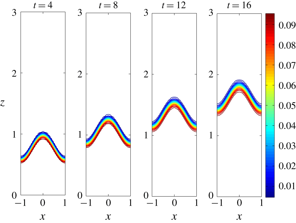
The linearized Boussinesq solution at four different dimensionless times $t=4$, 8, 12 and 16, started from a discontinuous approximation to the initial density profile (4.12) across the co-sinusoidal interface $z=h+\unicode[STIX]{x1D716}\cos (\unicode[STIX]{x03C0}x)$. Here, the wall angle is $\unicode[STIX]{x1D703}=\unicode[STIX]{x03C0}/3$, and $h=0.5$, $\unicode[STIX]{x1D716}=0.2$ and $S_{1}=0.1$. The density diffusion parameter is $\unicode[STIX]{x1D70E}=10^{-4}$.

A typical example of a linearized Boussinesq solution is illustrated in figure 3. Here, some contours of the linearized density function $S^{L}(x,z,t)$ in (5.22) are shown at the four different times $t=4$, 8, 12 and 16 in the region of the interface, for density values in the dimensionless interval $0.1<S^{L}<0.9$ so as to highlight the behaviour of this region. This is a solution obtained with $\unicode[STIX]{x1D70E}=10^{-4}$. The linearized Boussinesq theory developed in this Section clearly indicates that the initial profile for density does not change greatly as time progresses, except for some degree of diffusion of the initial front as it moves outward in the $z$-direction. Evidently linearization in this theory does not make adequate allowance for the effects of convection, particularly since shear is proportional to the small parameter $S_{1}$ as described in the assumed expansions (5.1), so that interfacial distortion is therefore a second-order effect in $S_{1}$. These nonlinear effects are addressed in the following section.

6 Local interface analysis in Boussinesq theory

The previous section demonstrates that, in Boussinesq theory, the linearized theory is largely unable to account for changes in the interfacial profile with time, with the result that the initial profile is predicted simply to move in the positive $z$-direction with only slight change of form. To study the destabilizing effects on the narrow interfacial zone as it progresses, a weakly nonlinear asymptotic analysis is required, and this is the topic of this present section.

The movement of the fluid in the direction of the positive $z$-axis was taken into account in § 5 by means of the moving coordinate (5.8). Here, we wish to focus on the narrow interfacial zone in more detail, and so we postulate that the density parameter $S_{1}$ in (2.1) is small, and define a new coordinate variable $Z$ in the interfacial zone, by means of the relation

(6.1)$$\begin{eqnarray}z=h+\unicode[STIX]{x1D6FD}t+S_{1}Z.\end{eqnarray}$$

The new coordinate $Z$ is an $O(1)$ quantity, and thus equation (6.1) ensures that the interfacial zone is narrow, with width of order $O(S_{1})$. The equations of the governing Boussinesq model (4.1)–(4.6) are now rewritten in terms of this coordinate $Z$.

After a careful scaling analysis of the solution variables, it is found to be appropriate to postulate behaviour of the form

(6.2)$$\begin{eqnarray}\displaystyle \left.\begin{array}{@{}c@{}}\unicode[STIX]{x1D6F9}(x,z,t)=\unicode[STIX]{x1D6FD}x+S_{1}^{2}\unicode[STIX]{x1D6F9}^{A}(x,Z,t),\\ u(x,z,t)=0+S_{1}U^{A}(x,Z,t),\\ w(x,z,t)=\unicode[STIX]{x1D6FD}+S_{1}^{2}W^{A}(x,Z,t),\\ S(x,z,t)=0+S_{1}S^{A}(x,Z,t),\end{array}\right\} & & \displaystyle\end{eqnarray}$$

in the moving interfacial zone. Here,

(6.3a,b)$$\begin{eqnarray}U^{A}=-\frac{\unicode[STIX]{x2202}\unicode[STIX]{x1D6F9}^{A}}{\unicode[STIX]{x2202}Z}\quad \text{and}\quad W^{A}=\frac{\unicode[STIX]{x2202}\unicode[STIX]{x1D6F9}^{A}}{\unicode[STIX]{x2202}x},\end{eqnarray}$$

and the vorticity $\unicode[STIX]{x1D701}$ defined in (4.5) now becomes

(6.4)$$\begin{eqnarray}\unicode[STIX]{x1D701}(x,z,t)=\unicode[STIX]{x1D6FA}^{A}+O(S_{1}^{2}),\end{eqnarray}$$

with

(6.5)$$\begin{eqnarray}\unicode[STIX]{x1D6FA}^{A}(x,Z,t)=\frac{\unicode[STIX]{x2202}U^{A}}{\unicode[STIX]{x2202}Z}.\end{eqnarray}$$

It is also necessary to scale the diffusion coefficients as

(6.6a,b)$$\begin{eqnarray}\frac{1}{R_{e}}=\unicode[STIX]{x1D708}_{0}S_{1}^{2}\quad \text{and}\quad \unicode[STIX]{x1D70E}=\unicode[STIX]{x1D70E}_{0}S_{1}^{2}.\end{eqnarray}$$

The parameters $R_{e}$ and $\unicode[STIX]{x1D70E}$ are respectively the Reynolds number and density diffusion coefficients, introduced in § 4. As a result of the scaling (6.6), the new constants $\unicode[STIX]{x1D708}_{0}$ and $\unicode[STIX]{x1D70E}_{0}$ are $O(1)$ in this moving interfacial layer.

It is now reasonably straightforward to show that the density equation (4.3) to order $O(S_{1})$ in the interfacial layer becomes simply

(6.7)$$\begin{eqnarray}\frac{\unicode[STIX]{x2202}S^{A}}{\unicode[STIX]{x2202}t}=\unicode[STIX]{x1D70E}_{0}\frac{\unicode[STIX]{x2202}^{2}S^{A}}{\unicode[STIX]{x2202}Z^{2}},\end{eqnarray}$$

and the vorticity equation (4.6) takes the $O(1)$ form

(6.8)$$\begin{eqnarray}\frac{\unicode[STIX]{x2202}\unicode[STIX]{x1D6FA}^{A}}{\unicode[STIX]{x2202}t}=\sin \unicode[STIX]{x1D703}\frac{\unicode[STIX]{x2202}S^{A}}{\unicode[STIX]{x2202}Z}+\unicode[STIX]{x1D708}_{0}\frac{\unicode[STIX]{x2202}^{2}\unicode[STIX]{x1D6FA}^{A}}{\unicode[STIX]{x2202}Z^{2}}.\end{eqnarray}$$

The question here is whether a small sinusoidal disturbance to the density profile in the interfacial zone is stable or otherwise, and so it is reasonable to take

(6.9)$$\begin{eqnarray}S^{A}(x,Z,t)=[1+\unicode[STIX]{x1D716}\cos (\unicode[STIX]{x03C0}x)]\exp [\unicode[STIX]{x1D70E}_{0}\unicode[STIX]{x1D706}^{2}t]\exp [-\unicode[STIX]{x1D706}Z]\end{eqnarray}$$

as an appropriate solution to the scaled density equation (6.7). At $Z=0$ at the initial time $t=0$, the average value of $S^{A}$ is $1$, which is consistent with the requirement that $S(x,z,t)=S_{1}$ between the wall at $z=0$ and the moving front $z=h+\unicode[STIX]{x1D6FD}t$, after the scalings (6.1) and (6.2) have been applied. Far ahead of the front, $S^{A}\rightarrow 0$ as $Z\rightarrow \infty$, as required for the outer limit of this inner expansion (6.2) in the moving interfacial region. Here, the parameter $\unicode[STIX]{x1D706}>0$ is some $O(1)$ constant.

Now that an asymptotic form (6.9) for the density function $S^{A}$ has been determined, the vorticity function $\unicode[STIX]{x1D6FA}^{A}$ may be obtained from (6.8), with the condition that there is no vorticity initially. This results in the solution

(6.10)$$\begin{eqnarray}\unicode[STIX]{x1D6FA}^{A}(x,Z,t)=\sin \unicode[STIX]{x1D703}q(t)[1+\unicode[STIX]{x1D716}\cos (\unicode[STIX]{x03C0}x)]\exp [-\unicode[STIX]{x1D706}Z],\end{eqnarray}$$

in which it is convenient to define the function

(6.11)$$\begin{eqnarray}q(t)=\left\{\begin{array}{@{}ll@{}}\displaystyle -\unicode[STIX]{x1D706}t\exp [\unicode[STIX]{x1D708}_{0}\unicode[STIX]{x1D706}^{2}t], & \text{if }\unicode[STIX]{x1D70E}_{0}=\unicode[STIX]{x1D708}_{0}\\ \displaystyle -[\exp [\unicode[STIX]{x1D708}_{0}\unicode[STIX]{x1D706}^{2}t]-\exp [\unicode[STIX]{x1D70E}_{0}\unicode[STIX]{x1D706}^{2}t]]/[(\unicode[STIX]{x1D708}_{0}-\unicode[STIX]{x1D70E}_{0})\unicode[STIX]{x1D706}], & \text{if }\unicode[STIX]{x1D70E}_{0}\neq \unicode[STIX]{x1D708}_{0}.\end{array}\right.\end{eqnarray}$$

From this asymptotic expression (6.10) for the scaled vorticity, the scaled streamfunction $\unicode[STIX]{x1D6F9}^{A}$ is now obtained from (6.2) to be

(6.12)$$\begin{eqnarray}\unicode[STIX]{x1D6F9}^{A}(x,Z,t)=-\frac{\sin \unicode[STIX]{x1D703}}{\unicode[STIX]{x1D706}^{2}}q(t)[1+\unicode[STIX]{x1D716}\cos (\unicode[STIX]{x03C0}x)]\text{e}^{-\unicode[STIX]{x1D706}Z},\end{eqnarray}$$

with the function $q(t)$ as defined in (6.11). Finally, the scaled velocity components $U^{A}$ and $W^{A}$ are obtained by differentiation of this solution (6.12), using (6.3). We observe that both velocity components $U^{A}$ and $W^{A}$ are zero at $Z=0$, rise to a maximum at some value $Z$ within the interfacial zone, and decay exponentially to zero as $Z\rightarrow 0$ far ahead of the front.

Figure 4.

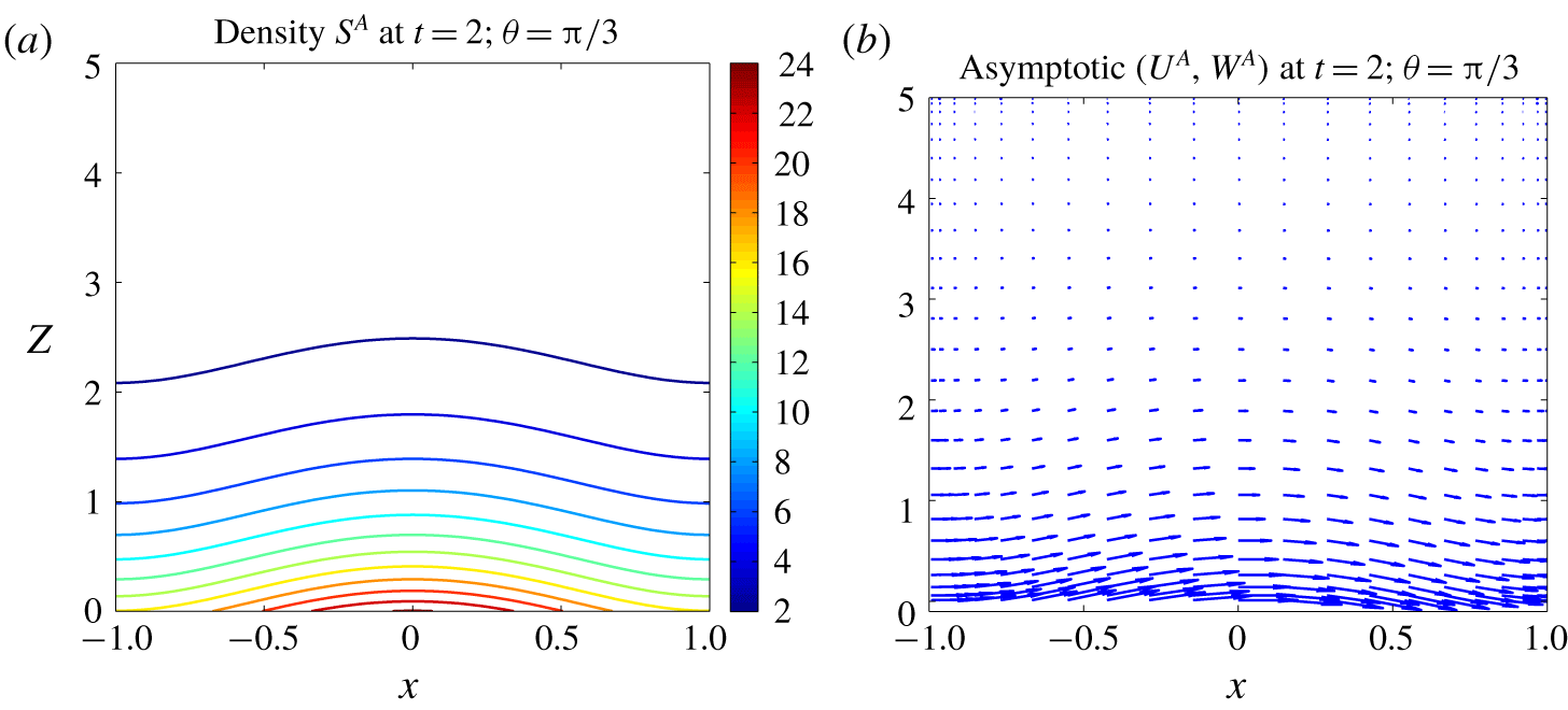
Scaled flow behaviour within the interfacial layer. (a) Density variation, and (b) scaled velocity vectors, illustrated for wall angle $\unicode[STIX]{x1D703}=\unicode[STIX]{x03C0}/3$, calculated from the asymptotic solution in § 6 at time $t=2$.

An indication of the solution behaviour within the interfacial region is presented in figure 4. In figure 4(a), contours of the scaled density function $S^{A}$ have been drawn for the case of an inclination angle $\unicode[STIX]{x1D703}=\unicode[STIX]{x03C0}/3$, evaluated from the expression (6.9). Far ahead of the front, there is only pure water, so that $S^{A}$ drops exponentially to zero as $Z\rightarrow \infty$, as expected. The scaled velocity components $U^{A}$ and $W^{A}$ have also been evaluated by direct differentiation of the streamfunction $\unicode[STIX]{x1D6F9}^{A}$ in (6.12), as indicated in (6.3), and the vector field $U^{A}\boldsymbol{e}_{\boldsymbol{x}}+W^{A}\boldsymbol{e}_{\boldsymbol{z}}$ for this same case is sketched in figure 4(b). Far upstream, these perturbation speeds fall to zero, as required, but in the interfacial zone itself, there is an overall motion of fluid parallel to the $x$-axis, down the slope. Consequently, a periodic disturbance at the interface, in the large-amplitude nonlinear results, might be expected to flow slightly faster nearer the wall than further away, giving the appearance of waves with crests that are distorted upstream. This will be investigated further numerically, in § 7.

7 Presentation of numerical results

In this section, we present and discuss some of the outcomes of this work. In all the cases to be discussed below, we have used $M=144$ Fourier modes and 720 mesh points in the interval $-1<x<1$ along the plate, and $N=288$ Fourier modes with 1440 numerical grid points in the direction orthogonal to the sloping boundary, over the interval $0<z<Z_{\infty }$. The outer computational boundary has been set at $Z_{\infty }=4$. In the numerical simulations, we have increased the number of grid points and spectral modes, and decreased the integration step size until no further changes to the main interface shape are apparent. This gives confidence that there is a high level of numerical accuracy. For the results presented here, the interface occurs over a narrow interval (typically $\unicode[STIX]{x0394}z\sim 0.1$); with our 1440 mesh points over $0<z<Z_{\infty }=4$ we thus have about 36 grid points across the interfacial zone, which is found to be capable of resolving this region very accurately. For definiteness, we have set the dimensionless inflow Froude number to be $\unicode[STIX]{x1D6FD}=0.07$ and the initial location of the interfacial zone at $h=0.5$. In addition, the amplitude $\unicode[STIX]{x1D716}$ of the initial disturbance is set at the value $\unicode[STIX]{x1D716}=0.2$ for all the results presented here, unless explicitly indicated otherwise.

Figure 5.

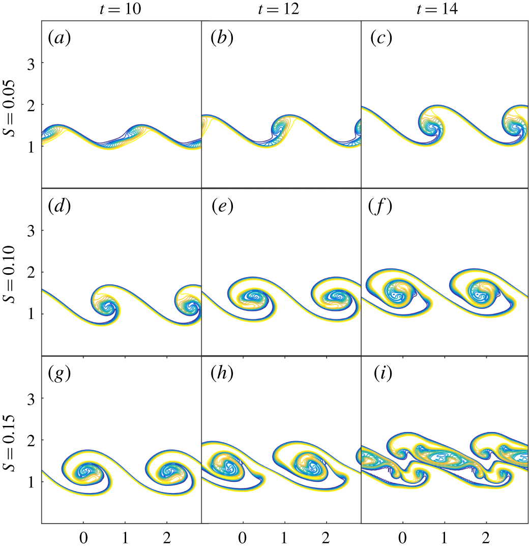
A comparison of the effect of density $S_{1}$ on the evolution of the interface. Contours of the density $S$ are shown at dimensionless times $t=10$ (a,d,g), $t=12$ (b,e,h) and $t=14$ (c,f,i). The density parameter is $S_{1}=0.05$ (a–c), 0.1 (d–f) and 0.15 (g–i). Results are shown over two wave periods $-1<x<3$ for ease of viewing. The two coordinates $x$ and $z$ are shown on the horizontal and vertical axes, respectively, and the scale on all axes is equal. The wall angle is $\unicode[STIX]{x1D703}=\unicode[STIX]{x03C0}/3$.

We begin by considering the influence of the density of the inflowing ground water. This is studied in figure 5, for the three different values of the density parameter $S_{1}=0.05$, 0.1 and 0.15 illustrated in rows (a–c), (d–f) and (g–i), respectively. For each value of the density, results are shown at the three (dimensionless) times $t=10$, 12 and 14, using (a,d,g), (b,e,h) and (c,f,i), respectively. In this figure, the wall angle is $\unicode[STIX]{x1D703}=\unicode[STIX]{x03C0}/3$. Contours of the density function $S(x,z,t)$ obtained from the spectral representation (4.8) are shown in each subplot, and the interfacial zone is at once evident as the narrow region over which contour lines are concentrated, as the density changes rapidly but smoothly from its wall value $S_{1}$ to its value $S=0$ in the purely fresh-water region far upstream. For ease of viewing, each diagram shows two wavelengths in the $x$-coordinate, over the double interval $-1<x<3$.

The top set of results in figure 5, with density $S_{1}=0.05$, show the interface evolving over the three times in a manner consistent with the behaviour of the K–H instability. Significant overturning of the interfacial profile is evident in the second picture at time $t=12$, giving a shape resembling a spilling breaker. At the last time $t=14$ on the right-hand side, a ‘cat’s eye’ spiral has started to develop, typical of the billowing structures formed in the K–H instability. At the higher density $S_{1}=0.1$ shown in row (d–f) of the diagrams in figure 5 the pattern is similar, except that the instability develops more rapidly at this higher density. This is consistent with the inviscid linearized theory of § 3, since from (3.17) the growth rate $\text{Re}\{\unicode[STIX]{x1D714}\}$ of the instability is predicted to increase with $S_{1}$, so that evolution occurs more rapidly. This is evident in figure 5, where for $S_{1}=0.1$ the interface at time $t=10$ has already overturned to about the same degree as at the later time $t=14$ in the row immediately above, with density $S_{1}=0.05$. Figure 5(g–i) also shows the interface at the same three times, but now at the still higher value $S_{1}=0.15$ of the upstream density. For this last case, the overturning interface has produced elaborate structures of some considerable complexity, as the initially more rapid development of the K–H instability predicted by the linearized theory (3.17) for this value of $S_{1}$ triggers nonlinear effects at earlier times for these large-amplitude billows.

Figure 6.

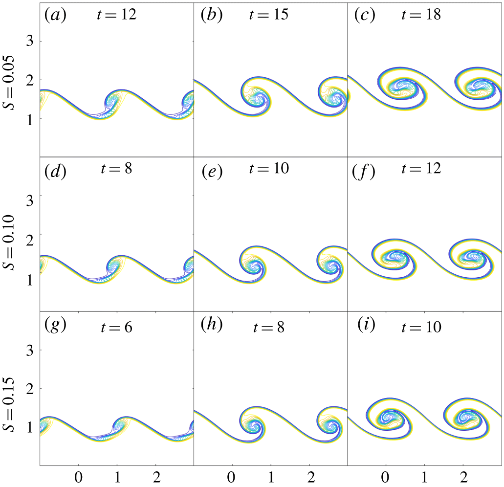
The combined effects of density and time on the development of the interface. The density parameter is $S_{1}=0.05$ (a–c), 0.1 (d–f) and 0.15 (g–i). Similar profiles are illustrated in each vertical column, but at different times for each value of the density parameter. Results are shown over two wave periods $-1<x<3$ for ease of viewing. The two coordinates $x$ and $z$ are shown on the horizontal and vertical axes, respectively, and the scale on all axes is equal. The wall angle is $\unicode[STIX]{x1D703}=\unicode[STIX]{x03C0}/3$.

It was observed in the discussion of figure 5 that increasing the density $S_{1}$ causes the interface to evolve more rapidly, and that, as a result, interface shapes obtained for one density $S_{1}$ may appear similar to those at a smaller density but at a later time. We have examined carefully the numerical results used in the creation of figure 5, and have attempted to illustrate these similarities in greater detail. Some sample results for the same parameter values as in figure 5 are shown in figure 6. In each vertical column the interface profiles have been chosen from our numerical solutions to be as similar in appearance as possible. However, as density $S_{1}$ increases, the similar wave profile is obtained at a correspondingly smaller time, as indicated in figure 6.

While the results in each of the three vertical columns in figure 6 are not identical, they are sufficiently similar to provoke the question as to whether some sort of scaling law might exist, by which it might be possible to predict at what time a particular wave profile might be obtained at some density value, knowing the time at which it occurred for some different density value. If this question can indeed be answered at all, it is very difficult to do so, based only on examination of numerical solution data. We have attempted to fit various scaling laws to the data for these three densities $S_{1}=0.05$, 0.1 and 0.15 obtained from our computer outputs, but have not been entirely successful. The best of our scaling-law estimations suggests that approximately the same interface profile will be obtained, at least for early to moderate times, if the parameter $\unicode[STIX]{x1D709}=S_{1}t^{n}$ remains invariant, where we estimate the exponent to be $n=1.75\pm 0.05$. We stress, however, that this is a purely empirical result, and is only approximate.

Figure 7.

A comparison of the effect of wall angle $\unicode[STIX]{x1D703}$ on the evolution of the interface. Contours of the density $S$ are shown at the four dimensionless times $t=10$, 14, 18 and $t=22$ in the corresponding four columns. The wall angle is $\unicode[STIX]{x1D703}=\unicode[STIX]{x03C0}/6$ (a–d), $\unicode[STIX]{x03C0}/4$ (e–h) and $\unicode[STIX]{x03C0}/3$ (i–l). Results are shown over two wave periods $-1<x<3$ for ease of viewing. The two coordinates $x$ and $z$ are shown on the horizontal and vertical axes, respectively, and the scale on all axes is equal. The density parameter is fixed at $S_{1}=0.1$.

We have also run the spectral method for the solution of the Boussinesq model in § 4 for a large number of different angles $\unicode[STIX]{x1D703}$ of the quarry wall relative to the horizontal. When $\unicode[STIX]{x1D703}=0$ and the wall is therefore horizontal, the system is seen to be essentially neutrally stable, although of course, the viscosity $1/R_{e}$ and diffusion $\unicode[STIX]{x1D70E}$ eventually lead to slow damping of disturbances, as in § 5. The interface rises up the $z$-axis so that its mean position is $z=h+\unicode[STIX]{x1D6FD}t$, and also undergoes seiching-type oscillations as it rises. For non-zero wall angle, however, there is a nett flow of the dense fluid down the sloping wall, so that K–H-type billows are observed. In the extreme limit $\unicode[STIX]{x1D703}=\unicode[STIX]{x03C0}$ there is a layer of denser fluid above, so that the flow becomes a pure Rayleigh–Taylor instability, and the interface develops rising bubbles of fresh water and downward fingers of dense fluid, in precisely the manner shown by Walters & Forbes (Reference Walters and Forbes2019).

Figure 7 illustrates the temporal evolution of the solution by presenting contour maps of the density $S$ at the four different times $t=10$, 14, 18 and 22, and for the three different wall angles $\unicode[STIX]{x1D703}=\unicode[STIX]{x03C0}/6$, $\unicode[STIX]{x03C0}/4$ and $\unicode[STIX]{x03C0}/3$. Figure 7(a–d) shows the results for the most shallow wall inclination $\unicode[STIX]{x1D703}=\unicode[STIX]{x03C0}/6$ at the four times. Once again, the development of a K–H-type instability is evident. Large amplitude billows have formed by time $t=18$, so that nonlinear effects are necessarily of paramount importance for such large disturbances to the mean interface level. These then make possible the formation of intricate entangled overturning structures at later times, and for $\unicode[STIX]{x1D703}=\unicode[STIX]{x03C0}/6$ at the last time $t=22$ shown, such complex patterns have begun to form. As the angle $\unicode[STIX]{x1D703}$ of the quarry wall is increased, figure 7 shows how the instability develops more rapidly so that, for the steepest case $\unicode[STIX]{x1D703}=\unicode[STIX]{x03C0}/3$, the interface has overturned and entrained the surrounding fluids to such an extent that it has resulted in the formation of a wide mixing layer between them.

Another feature that is apparent from figure 7 is the formation of a small, secondary wavelet in each wavelength. These are particularly noticeable at the shallower wall angles in the top two rows of results, at the earlier times $t=10$ and $t=14$. As time progresses, these are entrained into the larger billow in each wavelength, in a process that Carpenter et al. (Reference Carpenter, Tedford, Rahmani and Lawrence2010) refer to as ‘vortex pairing’ (although their work is more focussed on Holmboe instabilities). The larger of the two billows in each wavelength grows more rapidly than the smaller one, which is drawn into the overhanging portion of the larger vortex. For the intermediate times $t=14$, $t=18$ in figure 7, the remnants of this smaller billow are still visible within the overturning portion of the larger vortex, but eventually their presence is no longer able to be identified, as entrainment and mixing continue, and a more elaborate structure is formed. As the slope $\unicode[STIX]{x1D703}$ of the wall is increased, the relative size of the smaller, secondary vortex in each wavelength appears to reduce, and it is also entrained more rapidly into the faster-developing larger vortex. In the last row of results for angle $\unicode[STIX]{x1D703}=\unicode[STIX]{x03C0}/3$ in figure 7, the secondary vortex is essentially too small to be noticed and there is also no evidence of it in the overhanging portion of the larger billow.

In figures 5–7, the solution was started with a co-sinusoidal disturbance to the interface shape, as in (4.12). This represents a pure disturbance of just a single Fourier mode, and so it is of interest now to ascertain the degree to which the nonlinear evolution of the interface is affected by the choice of an initial condition comprised of many different Fourier modes. To do this, we have chosen to initialize the calculations from the (triangular) disturbance

(7.1)$$\begin{eqnarray}S(x,z,0)=\left\{\begin{array}{@{}ll@{}}0, & h+\unicode[STIX]{x1D716}(1-2|x|)<z<Z_{\infty }\\ S_{1}, & 0<z<h+\unicode[STIX]{x1D716}(1-2|x|).\end{array}\right.\end{eqnarray}$$

This is Fourier decomposed using the results (4.13), (4.14) as previously, to give initial values for the time-dependent Fourier coefficients. Since this function (7.1) is even in $x$, only a series of cosine functions is obtained, but now, there are infinitely many Fourier modes in the initial perturbation. In practice, we smooth the function (7.1) using Lanczos smoothing, so as to avoid discontinuities in the profile. We have likewise obtained a linearized solution to the Boussinesq model equations for this initial condition (7.1), as in § 5, but we do not discuss this further here, since it predicts essentially that the triangular density pattern simply moves up the $z$-axis, similar to the behaviour illustrated in figure 3, and this is only valid at early times.

Figure 8.

A comparison of the effect of different initial disturbance shapes on the evolution of the interface. Contours of the density $S$ are shown at the four dimensionless times $t=2$, 6, 10 and $t=14$ in the corresponding four columns. Row (a–d) corresponds to a solution started from the triangular wave pattern (7.1) at the four times, and (e–h) is the solution at the same four times, started from the purely co-sinusoidal disturbance (4.12). Row (i–l) corresponds to the ‘half-cosine’ profile in (7.2). Results are shown over two wave periods $-1<x<3$ for ease of viewing. The two coordinates $x$ and $z$ are shown on the horizontal and vertical axes, respectively, and the scale on all axes is equal. The density parameter is fixed at $S_{1}=0.1$ and the wall angle is $\unicode[STIX]{x1D703}=\unicode[STIX]{x03C0}/3$.

A comparison of the nonlinear results for the initial cosine profile (4.12) produced from a single Fourier mode and the initial triangular wave (7.1) is presented in figure 8. Row (a–d) represents results obtained at the four different times $t=2$, 6, 10 and $t=14$, starting from the triangular waveform (7.1). It was obtained using 128 modes and 720 points in the $x$-direction and 256 modes and 1440 points in the $z$-direction normal to the wall. Row (e–h) corresponds to the nonlinear solution that started from the purely co-sinusoidal density profile (4.12), and was generated using the same number of modes and points in $x$, but 288 modes and 1440 points in the $z$-direction. Remnants of the initially triangular shape are still evident in the solution at the earliest time $t=2$ shown in figure 8(a–d). As the two sets of results evolve, however, it is clear that they become more and more similar. For these two-dimensional shapes, therefore, it is evident that the shape of the initial profile has only a minor effect on the development of the K–H-type billows that form at the interface. Nevertheless, Klaassen & Peltier (Reference Klaassen and Peltier1991) have indicated that secondary instabilities can trigger a transition to three-dimensional flow from two-dimensional K–H instability, in which case small changes to the initial conditions may become important in fully three-dimensional flow.

It is perhaps reasonable to argue that initially co-sinusoidal and triangular interface shapes are not greatly dissimilar, and may be expected to evolve in a similar fashion. Therefore, as a further check, we have also investigated a periodic ‘half-cosine’ initial profile, of the form

(7.2)$$\begin{eqnarray}S(x,z,0)=\left\{\begin{array}{@{}ll@{}}0, & h+2\unicode[STIX]{x1D716}f_{H}(x)<z<Z_{\infty }\\ S_{1}, & 0<z<h+2\unicode[STIX]{x1D716}f_{H}(x)\end{array}\right.\end{eqnarray}$$

in which the shape of the interface is specified by the function

(7.3)$$\begin{eqnarray}f_{H}(x)=\left\{\begin{array}{@{}ll@{}}0, & 0.5<|x|<1\\ \frac{1}{2}(1+\cos (2\unicode[STIX]{x03C0}x)), & 0<|x|<0.5.\end{array}\right.\end{eqnarray}$$

This profile (7.2) is arguably a more realistic initial interface shape than the triangular case in (7.1), and still involves infinitely many Fourier modes in the representation of its interface (7.3). Again, this profile is smoothed in practice to avoid discontinuities, either by using Lanczos smoothing of its Fourier-series representation or else by embedding it in a formula similar to that used in (4.12).

Figure 8(i–l) shows the evolution of the density starting from the ‘half-cosine’ profile (7.2). In this case, there are slight differences in the shape of the profile as it evolves, since the smaller secondary wavelet in each wavelength is more pronounced. As time progresses, however, it becomes entrained into the larger overturning portion of the profile so that, at later times, there is little qualitative difference between the three sets of results in figure 8.

Figure 9.

The evolution of the interface from the same three initial disturbances as in figure 8, but at the four later times $t=18$, 22, 26, 30. Row (a–d) corresponds to a solution started from the triangular wave pattern (7.1), and (e–h) is the solution at the same four times, started from the purely co-sinusoidal disturbance (4.12). Row (i–l) corresponds to the ‘half-cosine’ profile in (7.2). Results are shown over two wave periods $-1<x<3$ for ease of viewing. The two coordinates $x$ and $z$ are shown on the horizontal and vertical axes, respectively, and the scale on all axes is equal. The density parameter is fixed at $S_{1}=0.1$ and the wall angle is $\unicode[STIX]{x1D703}=\unicode[STIX]{x03C0}/3$.

The role of the K–H instability in fluid mixing in the lake is studied in figure 9. Here, the solution was started from the same three initial disturbances as in figure 8, and the parameter values are the same. However, figure 9 shows the three sets of solutions at the four later times $t=18$, 22, 26 and $t=30$. The initial disturbance amplitude in each case was $\unicode[STIX]{x1D716}=0.2$, so that the entire interfacial zone was located within $2\unicode[STIX]{x1D716}=0.4$ units on the $z$-axis. As time progresses, the interface for the triangular (7.1) and the sinusoidal (4.12) initial conditions in the top two rows of diagrams in figure 8 first overhangs and then forms intricate K–H-type billows, as a result of the influence of nonlinearity on such large-amplitude structures. Similar behaviour is observed for the ‘half-cosine’ initial condition (7.2) in row (i–l), although in that case the secondary waves in each wavelength make the profiles more complex at earlier times. At the later times continued on in figure 9, however, the interface in each case clearly evolves further into an elaborate mixing zone, and by the last time $t=30$ shown here, strong entrainment of the upper fresh water has occurred, so that the width of the mixing layer in each case is now approximately 2 units on the $z$-axis. The vorticity originally generated in the interfacial zone by the mechanisms revealed in § 6 is further enhanced by nonlinearity, which is evidently responsible for the entrainment of the surrounding fresh water.

Figure 10.

The evolution of the interface width with time, drawn for the triangular initial disturbance (7.1) with a heavy solid line (black online), the cosine profile (4.12) with a lighter solid line (red online) and the ‘half-cosine’ profile (7.2) using a dashed line. The parameter values are the same as for figures 7 and 8.

Table 1.

This table shows the details used in each of the simulations. We note that cases 2, 6, 8 are actually the same simulation. Similarly, cases 9 and 13 are the same. These are included for ease of reference to the relevant figures. The inflow Froude number $\unicode[STIX]{x1D6FD}$ is set to 0.07 for all simulations, and the (artificial) upper boundary is placed at $Z_{\infty }=4$. The number of modes is always set to be one fifth of the number of points in the corresponding direction, and the number of points in $z$ is approximately twice the number of points in $x$, giving similar density of points in each dimension.

A careful analysis of the width of the mixing layer for each of the three initial profiles (7.1), (4.12) and (7.2), considered in figures 8 and 9, is presented in figure 10, for the same parameter values (refer to table 1). In this diagram, the billow width has been calculated, for each case, at 150 different times. This has been done at each time by having the computer evaluate the highest point on the upper interface and the lowest point on the lower interface and subtracting the two. Here, the ‘upper’ and ‘lower’ interfaces are defined numerically simply to be the heights $z$ at which the fluid density achieves its midpoint value. Thus, at the initial time $t=0$, the billow width in each case is calculated simply to be $2\unicode[STIX]{x1D716}=0.4$ by this process. The effects of the upper boundary at $Z_{\infty }=4$ can be seen in the results for the triangular (7.1) and co-sinusoidal (4.12) cases at later times in figure 10, where the billow width appears suddenly to decrease. This occurs essentially because the ‘top’ of the mixing region has reached the upper computational boundary $z=Z_{\infty }$ while the ‘bottom’ of this region continues to move upward due to the effects of buoyancy. These effects are visible in figure 9. The results shown in figure 10 summarize the outcomes of an enormous amount of computational time, and each of the three cases in figure 10 required approximately 40 hours run time on the high-speed machine built around parallel-processing graphics-card architecture, used in this study.

Figure 11.

The effect of initial amplitude $\unicode[STIX]{x1D716}$ upon the evolution of the interface. The solution was started using the ‘half-cosine’ profile (7.2), and results are shown for four different solutions, corresponding to four different starting amplitudes $\unicode[STIX]{x1D716}=0.025$, 0.05, 0.1 and 0.2. The interface is shown at the four times $t=0$ (initial profile), $t=10$, 20 and 30. Results are shown over two wave periods $-1<x<3$ for ease of viewing. The wall angle is $\unicode[STIX]{x1D703}=\unicode[STIX]{x03C0}/3$, the density parameter is $S_{1}=0.1$ and the inflow Froude number is $\unicode[STIX]{x1D6FD}=0.07$.

Figure 11 illustrates the way in which the evolution of the billow is affected by the initial amplitude $\unicode[STIX]{x1D716}$. Here, the interface is shown at four particular times, $t=0$ (initial condition), $t=10$, 20 and 30. In each case, the solution was started from the ‘half-cosine’ initial profile (7.2), and results are shown for four different initial amplitudes $\unicode[STIX]{x1D716}=0.025$, 0.05, 0.1 and 0.2. For this initial profile, the secondary wavelet in each wave period is much more pronounced than for the other two profiles in figures 8 and 9, and this affects the early stages of the evolution of the K–H billows. However, for each initial amplitude $\unicode[STIX]{x1D716}$, the mixing region widens rapidly as it entrains the surrounding fresh water, so that at later times the width of the mixing region is apparently not strongly affected by the initial amplitude of the disturbance.

Figure 12.

The evolution of the interface width with time, starting from the ‘half-cosine’ profile (7.2), for the same four initial amplitudes as in figure 11. Results are shown for $\unicode[STIX]{x1D716}=0.025$ (solid line, blue online), $\unicode[STIX]{x1D716}=0.05$ (chain dot, red online), $\unicode[STIX]{x1D716}=0.1$ (solid, brown online) and $0.2$ (dashed line, purple online).

This feature is studied in careful detail in figure 12. Here, the billow width for each of the solutions in figure 11 has been plotted as a function of time $t$. As with figure 10, each solution is presented in figure 12 at $150$ values of $t$, and each of the four cases shown required about 40 hours run time on our parallel-processing computer, details of which are given in Walters & Forbes (Reference Walters and Forbes2019). Figure 12 thus represents a summary of the results of an enormous amount of computational effort.

As is evident in figure 12, each of the four solutions shown starts with billow width equal simply to $2\unicode[STIX]{x1D716}$, consistent with initial condition (7.2) for this ‘half-cosine’ initial profile in each case. The billow widths retain the differences they were given initially, up until about time $t=15$ is reached. Thereafter, in each case the strong entrainment and mixing caused by the K–H instability results in knowledge of the initial amplitude being lost, so that there is no longer any meaningful difference in billow width as time progresses. As observed in connection with figure 10, the width of the interfacial region eventually becomes so large that it encounters the upper computational boundary at $z=Z_{\infty }=4$, and this starts to occur at around $t=25$. This artificial boundary could be moved out to a larger value of $z$, although this would require even greater computational resources to maintain this degree of accuracy, and so has not been pursued further here.

Figure 13.

The evolution of the interface profile, for the asymmetrically located ‘half-cosine’ initial disturbance at the four times $t=0$ (initial profile), $t=10$, 20 and 30. The initial amplitude was $\unicode[STIX]{x1D716}=0.2$, and the inflow Froude number is $\unicode[STIX]{x1D6FD}=0.07$. Results are shown over two wave periods $-1<x<3$ for ease of viewing.

So far, the wave profiles discussed have all been triggered by disturbances to the interface shape that are symmetric about the $z$-axis. To conclude this presentation of results, we illustrate in figure 13 the development of the interfacial zone, started from the ‘shifted half-cosine’ wave profile (7.2), but with the interface shape function (7.3) replaced with one that is shifted a quarter wavelength to the left. It is represented by the function

(7.4)$$\begin{eqnarray}f_{H}(x)=\left\{\begin{array}{@{}ll@{}}0, & -1<x<-0.75\\ \frac{1}{2}(1+\cos (2\unicode[STIX]{x03C0}[x+0.25])), & -0.75<x<0.25\\ 0, & 0.25<x<1.\end{array}\right.\end{eqnarray}$$

This replaces the shape function $f_{H}(x)$ used previously in (7.3), and as before, the Fourier coefficients in the representation (4.8) are obtained at $t=0$, and then subject to Lanczos smoothing (with Lanczos parameter 0.05). Figure 13 has been generated using $(M,N)=(144,288)$ Fourier modes and 720, 1440 mesh points in the $x$- and $z$-coordinates, respectively.

As anticipated, there are no essential qualitative differences between the ‘half-cosine’ profile asymmetrically placed, in figure 13, and the initially symmetrical profile of the same shape and amplitude illustrated in figure 11(m–p). Two complete wave profiles are shown in both these two diagrams, over the interval $-1<x<3$, and in both cases there is a pronounced secondary wavelet in each wavelength at time $t=10$. As time progresses, this wavelet is entrained by the larger disturbance as it rolls over. The interface entrains the surrounding fresh water in the same way in both these cases, so that the solution profiles at the later times $t=20$, $t=30$ in both figures 11(m–p) and 13 are almost identical.