



1 Introduction
For surface gravity wavepackets, the balancing role of the Eulerian return flow to compensate for the Stokes transport (Stokes Reference Stokes1847), which is divergent on the scale of the packet, is well-established (Longuet-Higgins & Stewart Reference Longuet-Higgins and Stewart1962; McIntyre Reference McIntyre1981; van den Bremer & Taylor Reference van den Bremer and Taylor2015) and has recently been extended to include the effect of underlying stratification (Haney & Young Reference Haney and Young2017). Vertically propagating internal wavepackets in a uniformly stratified fluid, on the other hand, do not have a Stokes drift, but only induce an Eulerian flow. Whereas the wave-induced flow for compact three-dimensional wavepackets consists of a purely horizontal localized circulation that translates with the wavepacket, known as the Bretherton flow, horizontally localized, spanwise infinite vertically propagating internal wavepackets resonate with the induced flow to generate long internal waves, whose vertical phase speed equals the vertical group velocity of the wavepacket (Bretherton Reference Bretherton1969; Tabaei & Akylas Reference Tabaei and Akylas2007; van den Bremer & Sutherland Reference van den Bremer and Sutherland2014, Reference van den Bremer and Sutherland2018).
Unlike vertically propagating internal gravity waves, horizontally modulated internal modes induce both a Stokes drift and an Eulerian flow. Focusing on periodic internal modes in uniform stratification, the Stokes drift has been computed by Thorpe (Reference Thorpe1968), and was shown to behave as a mode-
 $2n$
disturbance in the vertical, when formed in response to a mode-
 $n$
wave for positive integers
 $n$
. The occurrence of induced Eulerian flows was neglected in this case because of the lack of horizontal modulations of the waves. Al-Zanaidi & Dore (Reference Al-Zanaidi and Dore1976) showed that the Stokes drift in a thin-thermocline model was opposite in the interior of the thermocline compared to the drift in the outer layers. These authors also recognized that an Eulerian flow may significantly modify mass transport when multiple frequencies are present. The Eulerian flow of internal modes in uniform stratification was considered by McIntyre (Reference McIntyre1973). Grimshaw (Reference Grimshaw1977) considered the mean flow for arbitrary stratification, as well its effect on weakly nonlinear evolution. As in the case of the Stokes drift, McIntyre (Reference McIntyre1973) and Grimshaw (Reference Grimshaw1977) showed that a wavepacket composed of mode-
 $n$
waves induces an Eulerian flow with the structure of mode-
 $2n$
long waves. Grimshaw (Reference Grimshaw1977), and subsequently Grimshaw (Reference Grimshaw1981) and Liu & Benney (Reference Liu and Benney1981), considered the effect of this Eulerian mean flow on weakly nonlinear propagation by deriving a nonlinear Schrödinger equation, in which the Eulerian mean flow represents the nonlinear term. In particular, if the phase speed of the induced flow matches that of the group speed of the packet, then the induced horizontal flow in theory can become infinitely large and the scaling assumptions underlying the nonlinear Schrödinger equation are no longer valid. In response to this, Koop & Redekopp (Reference Koop and Redekopp1981) proposed a coupled pair of partial differential equations governing the exchange of energy between long and short internal waves subject to this resonance. When integrated numerically, this system compared well with their experiments, in which the long waves were generated separately and not induced by a packet of shorter waves.
For interfacial waves on a two-layer fluid, Hunt (Reference Hunt1961) computed the superharmonics at second (and third) order (reviewed in Thorpe (Reference Thorpe1968)), but not the Stokes drift or the Eulerian induced flow. Keady (Reference Keady1971), who was interested in the upstream response to a small body (or equivalently a weak dipole) moving at the interface between two layers of different density and depth, formulated equations for the Eulerian mean flow and the response of the wave-averaged interface, but focused solely on the latter. In Keady (Reference Keady1971), a body moving at constant speed does work on the fluid, and the wave-averaged interface thus jumps discretely at the position where the impulse is applied and displaces into the shallower layer just behind the impulse. Grimshaw & Pullin (Reference Grimshaw and Pullin1985) derived a nonlinear Schrödinger equation describing the modulational stability of interfacial waves in a two-layer fluid and in doing so formulated equations describing the wave-induced Eulerian mean flow, which constitutes the nonlinear term in their nonlinear Schrödinger equation. More recently, Song (Reference Song2004) evaluated the complete second-order solution in response to a summation of linear waves with different frequencies. The second-order frequency difference components in Song (Reference Song2004) correspond to the wave-induced Eulerian mean flow.
This paper examines the total Lagrangian transport, as made up from the Stokes drift and the induced Eulerian flow, by two-dimensional, Boussinesq, horizontally modulated, vertically confined (or guided) internal waves in arbitrary stratification. We consider solutions for four special cases: interfacial waves in a two-layer fluid (exploring in detail the implications of Keady (Reference Keady1971) and Grimshaw & Pullin (Reference Grimshaw and Pullin1985)); internal waves in symmetric and asymmetric top-hat stratification in which the density varies linearly in the middle layer and is constant above and below (designed to draw the connection between previous studies of two-layer and uniform stratification); and internal waves in exponential stratification (designed to be more representative of oceanic stratification).
The paper is laid out as follows. After introducing the governing equations in § 2, theoretical solutions from perturbation theory are presented in § 3. In § 4 solutions are found for the special cases, in analytic form for wavepackets in a two-layer fluid and in top-hat stratification and computed numerically through a Galerkin analysis for exponential stratification. In § 5, we describe the set-up of numerical simulations and compare their results to theoretical predictions. We draw conclusions in § 6.
2 Governing equations
We restrict ourselves to the examination of two-dimensional, vertically confined (or guided), Boussinesq internal waves, neglecting the effects of background rotation, diffusion and viscosity. The equations of motion are given by the laws of conservation of momentum, internal energy and volume for an incompressible fluid in the
 $x$
–
 $z$
plane
 $$\begin{eqnarray}{\displaystyle \frac{D\boldsymbol{u}}{Dt}}=-{\displaystyle \frac{1}{\unicode[STIX]{x1D70C}_{ref}}}\unicode[STIX]{x1D735}p+b\hat{\boldsymbol{z}},\quad {\displaystyle \frac{Db}{Dt}}=-N^{2}w,\quad \unicode[STIX]{x1D735}\boldsymbol{\cdot }\boldsymbol{u}=0,\end{eqnarray}$$
in which
 $b=-g\unicode[STIX]{x1D70C}/\unicode[STIX]{x1D70C}_{ref}$
is the buoyancy,
 $\boldsymbol{u}=(u,w)$
is the velocity vector with components in the
 $\hat{\boldsymbol{x}}$
and
 $\hat{\boldsymbol{z}}$
directions,
 $\unicode[STIX]{x1D70C}$
and
 $p$
are respectively the wave fluctuation density and pressure,
 $g$
is gravity and
 $\unicode[STIX]{x1D70C}_{ref}$
is the characteristic density. The right-hand side of (2.1b
) involves the squared buoyancy frequency, which is related to the gradient of the background or hydrostatic equilibrium density
 $\unicode[STIX]{x1D70C}_{0}(z)$
by
 $N^{2}=-(g/\unicode[STIX]{x1D70C}_{ref})\,\text{d}\unicode[STIX]{x1D70C}_{0}/\text{d}z$
. In a uniformly stratified fluid
 $N^{2}$
is a positive constant. The total density
 $\unicode[STIX]{x1D70C}_{tot}$
is given by the sum of the background density and the wave fluctuation density:
 $\unicode[STIX]{x1D70C}_{tot}(\boldsymbol{x},t)=\unicode[STIX]{x1D70C}_{0}(z)+\unicode[STIX]{x1D70C}(\boldsymbol{x},t)$
. Similarly,
 $p_{tot}(\boldsymbol{x},t)=p_{0}(z)+p(\boldsymbol{x},t)$
, where the background hydrostatic pressure
 $p_{0}$
can be found by solving
 $\text{d}p_{0}/\text{d}z=-\unicode[STIX]{x1D70C}_{0}(z)g$
. We orient the horizontal axis so that the horizontal phase velocity of the wave is in the direction of
 $\hat{\boldsymbol{x}}$
, and
 $\hat{\boldsymbol{y}}$
represents the spanwise direction. Because we consider only waves that are two-dimensional or spanwise uniform, we can define the streamfunction
 $\unicode[STIX]{x1D713}$
, so that
 $(u,w)=(-\unicode[STIX]{x2202}_{z}\unicode[STIX]{x1D713},~\unicode[STIX]{x2202}_{x}\unicode[STIX]{x1D713})$
.
Equations (2.1a–c
) can be combined and written as a linear operator
 $L$
acting on
 $\unicode[STIX]{x1D713}$
forced by nonlinear terms
 ${\mathcal{N}}$
:
 $$\begin{eqnarray}\underbrace{\big(\unicode[STIX]{x2202}_{tt}(\unicode[STIX]{x2202}_{xx}+\unicode[STIX]{x2202}_{zz})+N^{2}\unicode[STIX]{x2202}_{xx}\big)}_{\equiv ~L}\unicode[STIX]{x1D713}=\underbrace{\unicode[STIX]{x1D735}\boldsymbol{\cdot }\left[\unicode[STIX]{x2202}_{t}(\unicode[STIX]{x1D701}\boldsymbol{u})-\unicode[STIX]{x2202}_{x}(b\boldsymbol{u})\right]}_{\equiv ~N},\end{eqnarray}$$
in which
 $\unicode[STIX]{x1D701}=\unicode[STIX]{x2202}_{z}u-\unicode[STIX]{x2202}_{x}w$
denotes the spanwise vorticity.
3 Perturbation theory
We consider quasi-monochromatic waves of small amplitude. The condition that the wave amplitude is small is expressed by
 $\unicode[STIX]{x1D6FC}\equiv k||A||\ll 1$
, where
 $a_{0}\equiv ||A||$
is the maximum amplitude of the vertical displacement of the waves and
 $k$
the horizontal wavenumber. Below, we will consider the first two orders. The total Lagrangian velocity is given by the sum of the Stokes drift and the induced Eulerian flow, which both arise at second order in
 $\unicode[STIX]{x1D6FC}$
(cf. Bühler Reference Bühler2014):
 $$\begin{eqnarray}\boldsymbol{u}_{L}=\boldsymbol{u}_{S}+\boldsymbol{u}_{E},\end{eqnarray}$$
where we have omitted the superscripts normally denoting the order in
 $\unicode[STIX]{x1D6FC}$
.
3.1 Linear solutions:
 $O(\unicode[STIX]{x1D6FC})$

Linear or ‘small-amplitude’ internal waves satisfy
 $L\unicode[STIX]{x1D713}^{(1)}=0$
(cf. (2.2)), in which the superscript denotes the order in
 $\unicode[STIX]{x1D6FC}$
. Crucially, we require the stratification
 $N$
to be a continuous function of
 $z$
in order for the system (2.1) and thus (2.2) to hold. In other words, care must be taken at interfaces, where the density jumps discretely and
 $N$
is locally unbounded. We suppose that, rather than being horizontally periodic, the disturbance is manifest as a quasi-monochromatic wavepacket modulated in
 $x$
about a central wavenumber
 $k$
and frequency
 $\unicode[STIX]{x1D714}$
. While the wave crests advance at the phase speed
 $c_{p}=\unicode[STIX]{x1D714}/k$
, the wavepacket as a whole translates in the
 $x$
-direction at the group velocity
 $c_{g}=\unicode[STIX]{x2202}\unicode[STIX]{x1D714}/\unicode[STIX]{x2202}k$
, while slowly dispersing. Explicitly, we assume the vertical displacement field and the streamfunction respectively have the form
 $$\begin{eqnarray}\displaystyle & \displaystyle \unicode[STIX]{x1D702}^{(1)}=\{A_{0}(X,T)\hat{\unicode[STIX]{x1D702}}_{0}(z)+\unicode[STIX]{x1D700}A_{1}(X,T)\hat{\unicode[STIX]{x1D702}}_{1}(z)\}\exp [\imath (kx-\unicode[STIX]{x1D714}t)]+O(\unicode[STIX]{x1D6FC}\unicode[STIX]{x1D700}^{2}), & \displaystyle\end{eqnarray}$$
 $$\begin{eqnarray}\displaystyle & \displaystyle \unicode[STIX]{x1D713}^{(1)}=\{P_{0}(X,T)\hat{\unicode[STIX]{x1D713}}_{0}(z)+\unicode[STIX]{x1D700}P_{1}(X,T)\hat{\unicode[STIX]{x1D713}}_{1}(z)\}\exp [\imath (kx-\unicode[STIX]{x1D714}t)]+O(\unicode[STIX]{x1D6FC}\unicode[STIX]{x1D700}^{2}), & \displaystyle\end{eqnarray}$$
in which it is understood that the actual fields are given by the real part of these expressions. The quantities
 $\hat{\unicode[STIX]{x1D702}}_{0}(z)$
,
 $\hat{\unicode[STIX]{x1D702}}_{1}(z)$
,
 $\hat{\unicode[STIX]{x1D713}}_{0}(z)$
and
 $\hat{\unicode[STIX]{x1D713}}_{1}(z)$
denote the (dimensionless) vertical structure functions. To obtain leading-order solutions for the induced mean flow, it is only necessary to consider the first two terms in the multiple-scale expansion in the small parameter
 $\unicode[STIX]{x1D700}\equiv (|k|\unicode[STIX]{x1D70E})^{-1}$
. Setting
 $0<\unicode[STIX]{x1D700}\ll 1$
ensures the horizontal wavelength of the waves is much smaller than the horizontal extent of the wavepacket
 $\unicode[STIX]{x1D70E}$
, so that the wavepacket is quasi-monochromatic. The envelopes
 $A_{0}$
,
 $A_{1}$
,
 $P_{0}$
and
 $P_{1}$
depend upon the slow scales
 $X=\unicode[STIX]{x1D700}(x-c_{g}t)$
and
 $T=\unicode[STIX]{x1D700}^{2}t$
. The corresponding time
 $T$
for evolution of the wavepacket in this translating frame is of order
 $\unicode[STIX]{x1D700}^{2}$
, representing the relatively slow dispersion of the wavepacket. In fact, dispersion does not influence the induced flows at leading order, as will be evident below. Substituting the proposed linear solutions (3.2)–(3.3) into (2.1), equations can be obtained describing these and related fields at the first two orders in
 $\unicode[STIX]{x1D700}$
. Somewhat arbitrarily, all the polarization relations are expressed in terms of
 $A_{0}$
,
 $\hat{\unicode[STIX]{x1D702}}_{0}$
and
 $\hat{\unicode[STIX]{x1D702}}_{1}$
, as summarized in table 1.
Expressions for the linear,
 $O(\unicode[STIX]{x1D6FC})$
, fields at order
 $\unicode[STIX]{x1D700}^{0}$
(second column) and order
 $\unicode[STIX]{x1D700}^{1}$
(third column) in a stratified (
 $N\neq 0$
) or unstratified layer (
 $N=0$
). The fields are given in terms of the amplitude envelope and its
 $X$
-derivative, and in terms of the vertical structure functions of the vertical displacement and its derivatives (cf. (3.2)). The actual fields are found by adding the
 $O(\unicode[STIX]{x1D700}^{0})$
and
 $O(\unicode[STIX]{x1D700}^{1})$
terms, multiplying by
 $\exp [\imath (kx-\unicode[STIX]{x1D714}t)]$
and taking the real part of the result. We have defined
 $\unicode[STIX]{x1D712}\equiv c_{g}/c_{p}$
. Note that the velocity potential
 $\unicode[STIX]{x1D719}$
only exists in layers without stratification (
 $N=0$
).

3.1.1 Vertical structure functions
Evidently, the vertical structure functions
 $\hat{\unicode[STIX]{x1D702}}_{0}$
,
 $\hat{\unicode[STIX]{x1D702}}_{1}$
,
 $\hat{\unicode[STIX]{x1D713}}_{0}$
and
 $\hat{\unicode[STIX]{x1D713}}_{1}$
cannot be chosen independently. In fact, by considering the linearized (in
 $\unicode[STIX]{x1D6FC}$
) governing equations (2.1) at zeroth order in
 $\unicode[STIX]{x1D700}$
, it can be shown that
 $\hat{\unicode[STIX]{x1D702}}_{0}=\hat{\unicode[STIX]{x1D713}}_{0}$
, and both vertical structure functions satisfy the same modal equation:
 $$\begin{eqnarray}{\displaystyle \frac{\text{d}^{2}\,\hat{\unicode[STIX]{x1D702}}_{0}}{\text{d}z^{2}}}+\left({\displaystyle \frac{N^{2}}{\unicode[STIX]{x1D714}^{2}}}-1\right)k^{2}\hat{\unicode[STIX]{x1D702}}_{0}=0.\end{eqnarray}$$
For stratification prescribed by
 $N^{2}(z)$
, this differential eigenvalue problem can be solved for
 $\hat{\unicode[STIX]{x1D702}}_{0}$
and the corresponding dispersion relation
 $\unicode[STIX]{x1D714}(k)$
, both of which depend upon the vertical mode number. Crucially, equation (3.4) must be solved subject to no-flow boundary conditions at the two confining horizontal walls to ensure the solution propagates only horizontally. At the next order in
 $\unicode[STIX]{x1D700}$
, we obtain the differential equation describing the vertical structure function
 $\hat{\unicode[STIX]{x1D702}}_{1}$
, as well as
 $\hat{\unicode[STIX]{x1D713}}_{1}$
 $$\begin{eqnarray}\left({\displaystyle \frac{1}{k^{2}}}{\displaystyle \frac{\text{d}^{2}}{\text{d}z^{2}}}+{\displaystyle \frac{N^{2}}{\unicode[STIX]{x1D714}^{2}}}-1\right)\hat{\unicode[STIX]{x1D702}}_{1}=2\left((1-\unicode[STIX]{x1D712}){\displaystyle \frac{N^{2}}{\unicode[STIX]{x1D714}^{2}}}-1\right)\hat{\unicode[STIX]{x1D702}}_{0},\end{eqnarray}$$
where we have defined
 $\unicode[STIX]{x1D712}\equiv c_{g}/c_{p}$
. We further find that
 $\hat{\unicode[STIX]{x1D702}}_{1}=\hat{\unicode[STIX]{x1D713}}_{1}-(1-\unicode[STIX]{x1D712})\hat{\unicode[STIX]{x1D702}}_{0}$
. Alternatively, the compatibility condition (3.5) can be regarded as a definition of the group velocity (see appendix B for details). Below, we will show that only the vertical structure function
 $\hat{\unicode[STIX]{x1D702}}_{0}$
is required to compute the Stokes drift and the induced Eulerian flow.
3.1.2 Stokes drift
One can follow the methodology first performed by Stokes (Reference Stokes1847) to derive the order amplitude-squared displacement of fluid parcels by a horizontally periodic internal mode. Generally, the Stokes drift is given by
 $$\begin{eqnarray}\boldsymbol{u}_{S}\equiv \overline{\boldsymbol{u}_{x}^{(1)}\unicode[STIX]{x1D709}^{(1)}+\boldsymbol{u}_{z}^{(1)}\unicode[STIX]{x1D702}^{(1)}},\end{eqnarray}$$
in which the
 $x$
and
 $z$
subscripts denote partial derivatives,
 $\unicode[STIX]{x1D709}$
and
 $\unicode[STIX]{x1D702}$
are the horizontal and vertical displacements, respectively, and the overline denotes averaging over the fast time scales of the waves. From the polarization relations for internal modes in table 1 and using (3.4), we find the following leading order
 $$\begin{eqnarray}u_{S}={\displaystyle \frac{1}{4}}c_{p}|A_{0}|^{2}{\displaystyle \frac{\text{d}^{2}\hat{\unicode[STIX]{x1D702}}_{0}^{2}}{\text{d}z^{2}}},\quad w_{S}=-{\displaystyle \frac{1}{4}}c_{p}(1+\unicode[STIX]{x1D712})\unicode[STIX]{x1D700}\unicode[STIX]{x2202}_{X}|A_{0}|^{2}{\displaystyle \frac{\text{d}\hat{\unicode[STIX]{x1D702}}_{0}^{2}}{\text{d}z}}.\end{eqnarray}$$
Equation (3.7a ) corresponds to that derived by Thorpe (Reference Thorpe1968) (his appendix 6).
We note in passing that the Stokes drift (3.7) is divergent (
 $\unicode[STIX]{x1D735}\boldsymbol{\cdot }\boldsymbol{u}_{S}\neq 0$
), which is generally true for Lagrangian velocities even in incompressible fluids. Indeed, we can readily confirm that (3.7) satisfies the identity for volume conservation
 $\unicode[STIX]{x1D735}\boldsymbol{\cdot }\boldsymbol{u}_{S}=(1/2)\unicode[STIX]{x2202}_{tzz}\overline{(\unicode[STIX]{x1D702}^{(1)})^{2}}$
from generalized Lagrangian-mean theory (equation (9.4) of Andrews & McIntyre (Reference Andrews and McIntyre1978)), shown here correct to leading order for our case (see also McIntyre (Reference McIntyre1988) for a discussion of the analogous effect for surface waves).
3.2 Second-order solutions:
$O(\unicode[STIX]{x1D6FC}^{2})$

The induced Eulerian is found by substituting the linear polarization relations from table 1 into the right-hand side of (2.2) keeping only the slow response at order amplitude squared. In doing so, superharmonic terms involving
 $\exp [\pm 2\imath (kx-\unicode[STIX]{x1D714}t)]$
are neglected as they do not influence the mean Lagrangian transport. After some algebra (see appendix A), we find that the forcing is given by (see also section 4 of Grimshaw (Reference Grimshaw1977))
 $$\begin{eqnarray}\overline{{\mathcal{N}}}=\unicode[STIX]{x1D700}^{2}c_{p}\left[{\displaystyle \frac{1}{4}}\left(1+2\unicode[STIX]{x1D712}\right)(1-\unicode[STIX]{x1D712})N^{2}{\displaystyle \frac{\text{d}\hat{\unicode[STIX]{x1D702}}_{0}^{2}}{\text{d}z}}-{\displaystyle \frac{1}{2}}\unicode[STIX]{x1D712}^{2}\,{\displaystyle \frac{\text{d}N^{2}}{\text{d}z}}\,\hat{\unicode[STIX]{x1D702}}_{0}^{2}\right]\unicode[STIX]{x2202}_{XX}|A_{0}|^{2},\end{eqnarray}$$
where we note that only the zeroth-order vertical structure function
 $\hat{\unicode[STIX]{x1D702}}_{0}$
plays a role. The streamfunction
 $\overline{\unicode[STIX]{x1D713}}^{(2)}$
describing the order amplitude-squared flows induced by this nonlinear self-interaction of the wavepacket satisfies
 $L\overline{\unicode[STIX]{x1D713}}^{(2)}=\overline{{\mathcal{N}}}$
, with
 $L$
given on the left-hand side of (2.2). The expression for the
 $O(\unicode[STIX]{x1D6FC}^{2})$
induced buoyancy is given from (2.1b
) to be
 $\unicode[STIX]{x2202}_{t}\overline{b}^{(2)}=-N^{2}\unicode[STIX]{x2202}_{x}\overline{\unicode[STIX]{x1D713}}^{(2)}-\unicode[STIX]{x2202}_{x}(\overline{u^{(1)}b^{(1)}})-\unicode[STIX]{x2202}_{z}(\overline{w^{(1)}b^{(1)}})$
. Again using the polarization relations in table 1, we find
 $$\begin{eqnarray}\overline{b}^{(2)}={\displaystyle \frac{1}{c_{g}}}N^{2}\overline{\unicode[STIX]{x1D713}}^{(2)}+{\displaystyle \frac{1}{4}}\left[\left(1-{\displaystyle \frac{1}{\unicode[STIX]{x1D712}}}\right)N^{2}\,{\displaystyle \frac{\text{d}\hat{\unicode[STIX]{x1D702}}_{0}^{2}}{\text{d}z}}+{\displaystyle \frac{\text{d}N^{2}}{\text{d}z}}\,\hat{\unicode[STIX]{x1D702}}_{0}^{2}\right]|A_{0}|^{2}.\end{eqnarray}$$
From (3.9) we can obtain an expression for the mean displacement of the equidensity lines
 $$\begin{eqnarray}\overline{\unicode[STIX]{x1D702}}^{(2)}=-{\displaystyle \frac{1}{c_{g}}}\overline{\unicode[STIX]{x1D713}}^{(2)}-{\displaystyle \frac{1}{4}}\left[\left(1-{\displaystyle \frac{1}{\unicode[STIX]{x1D712}}}\right)\,{\displaystyle \frac{\text{d}\hat{\unicode[STIX]{x1D702}}_{0}^{2}}{\text{d}z}}+{\displaystyle \frac{1}{N^{2}}}{\displaystyle \frac{\text{d}N^{2}}{\text{d}z}}\,\hat{\unicode[STIX]{x1D702}}_{0}^{2}\right]|A_{0}|^{2},\end{eqnarray}$$
in which the last term can be neglected where
 $N^{2}$
is constant.
Assuming strong stratification (
 $N/\unicode[STIX]{x1D714}=O(1)$
), examining a solution that evolves on the slow scale
 $X=\unicode[STIX]{x1D700}(x-c_{g}t)$
and then extracting the leading-order terms in the linear operator, up to
 $O(\unicode[STIX]{x1D6FC}^{2}\unicode[STIX]{x1D700}^{2})$
, gives from (2.2)
 $$\begin{eqnarray}\unicode[STIX]{x1D700}^{2}\unicode[STIX]{x2202}_{XX}(c_{g}^{2}\unicode[STIX]{x2202}_{zz}+N^{2})\overline{\unicode[STIX]{x1D713}}^{(2)}(X,z)=\overline{{\mathcal{N}}}.\end{eqnarray}$$
where
 $\overline{{\mathcal{N}}}$
is given by (3.8). Integrating twice in
 $X$
, we see that
 $\overline{\unicode[STIX]{x1D713}}^{(2)}$
can be represented by
 $$\begin{eqnarray}\overline{\unicode[STIX]{x1D713}}^{(2)}(X,z)=N_{0}|A_{0}(X)|^{2}\unicode[STIX]{x1D6F9}(z),\end{eqnarray}$$
in which
 $\unicode[STIX]{x1D6F9}(z)$
is the (non-dimensional) vertical structure of the induced flow and
 $N_{0}$
is a characteristic value of the background buoyancy frequency. Thus the vertical structure of the induced streamfunction is given by the solution of
 $$\begin{eqnarray}c_{g}^{2}\unicode[STIX]{x1D6F9}^{\prime \prime }+N^{2}\unicode[STIX]{x1D6F9}={\displaystyle \frac{c_{p}}{N_{0}}}\left\{\left[{\displaystyle \frac{1}{4}}\left(1+2\unicode[STIX]{x1D712}\right)\left(1-\unicode[STIX]{x1D712}\right)\right]\,N^{2}\,{\displaystyle \frac{\text{d}\hat{\unicode[STIX]{x1D702}}_{0}^{2}}{\text{d}z}}-{\displaystyle \frac{1}{2}}\unicode[STIX]{x1D712}^{2}\,{\displaystyle \frac{\text{d}N^{2}}{\text{d}z}}\,\hat{\unicode[STIX]{x1D702}}_{0}^{2}\right\}.\end{eqnarray}$$
Once
 $\unicode[STIX]{x1D6F9}(z)$
has been found from (3.13), the induced horizontal flow can be computed as
 $$\begin{eqnarray}\overline{u}^{(2)}=-N_{0}|A_{0}|^{2}{\displaystyle \frac{\text{d}\,\unicode[STIX]{x1D6F9}}{\text{d}z}}.\end{eqnarray}$$
4 Solutions for special cases
In this section, we solve for the Stokes drift
 $u_{S}$
and the induced Eulerian flow
 $u_{E}\equiv \overline{u}^{(2)}$
for the special cases illustrated in figure 1. We begin by finding analytic solutions for interfacial waves in a two-layer fluid (§ 4.1). We then consider internal waves in symmetric top-hat stratification (§ 4.2), comparing and contrasting the solutions with those for interfacial waves in a symmetric two-layer fluid in § 4.1 and for internal waves in uniform stratification (McIntyre Reference McIntyre1973). The case of asymmetric top-hat stratification is examined next (§ 4.3), wherein it is shown that, like in the two-layer case, the induced Eulerian flow becomes very large for shallow internal waves even if the stratification is only moderately asymmetric. Finally, we compute solutions for the case of internal waves in exponential stratification (§ 4.4).
Illustration of the special cases examined: (a) interfacial waves in a two-layer fluid, (b) internal waves in a three-layer fluid with top-hat stratification
 $N$
and (c) internal waves in exponential stratification with e-folding depth
 $\unicode[STIX]{x1D70E}_{e}$
. In all cases the total height of the domain is
 $H$
and
 $D=H/2$
. In (a) and (b)
 $z$
is defined upwards from the vertical centre of the domain.

4.1 Two-layer fluid
We consider a two-layer Boussinesq fluid with upper-layer depth
 $D_{+}$
and density
 $\unicode[STIX]{x1D70C}_{+}$
and lower-layer depth
 $D_{-}$
and density
 $\unicode[STIX]{x1D70C}_{-}$
. In this case, the forcing equation (2.2) readily reduces to Laplace’s equation in the two layers:
 $\unicode[STIX]{x1D735}^{2}\unicode[STIX]{x1D719}_{+}=0$
for
 $z>\unicode[STIX]{x1D6FF}+\unicode[STIX]{x1D702}_{I}(x,t)$
and
 $\unicode[STIX]{x1D735}^{2}\unicode[STIX]{x1D719}_{-}=0$
for
 $z<\unicode[STIX]{x1D6FF}+\unicode[STIX]{x1D702}_{I}(x,t)$
, where
 $\unicode[STIX]{x1D702}_{I}(x,t)\equiv \unicode[STIX]{x1D702}(x,z=\unicode[STIX]{x1D6FF},t)$
denotes the vertical displacement of the interface with neutral position
 $z=\unicode[STIX]{x1D6FF}$
, and
 $+$
and
 $-$
denote the top and bottom layers, respectively. The total depth is
 $H$
,
 $D=H/2$
,
 $D_{+}=D-\unicode[STIX]{x1D6FF}$
, and
 $D_{-}=D+\unicode[STIX]{x1D6FF}$
. These two equations must be solved subject to no-flow boundary conditions at the top and bottom and three boundary conditions at the interface. The boundary conditions are, respectively, a kinematic boundary condition for the velocities in the top layer, a kinematic boundary condition for the velocities in the bottom layer and a dynamic boundary condition setting the pressure at either side of the interface to be equal, given here using Bernoulli’s equation:
 $$\begin{eqnarray}\displaystyle & \displaystyle {\displaystyle \frac{\unicode[STIX]{x2202}\unicode[STIX]{x1D702}_{I}}{\unicode[STIX]{x2202}t}}+u_{\pm }{\displaystyle \frac{\unicode[STIX]{x2202}\unicode[STIX]{x1D702}_{I}}{\unicode[STIX]{x2202}x}}-w_{\pm }=0\quad \text{for }z=\unicode[STIX]{x1D6FF}+\unicode[STIX]{x1D702}_{I}(x,t), & \displaystyle\end{eqnarray}$$
 $$\begin{eqnarray}\displaystyle & \displaystyle g^{\prime }\unicode[STIX]{x1D702}_{I}={\displaystyle \frac{\unicode[STIX]{x2202}\unicode[STIX]{x1D719}_{+}}{\unicode[STIX]{x2202}t}}+{\displaystyle \frac{1}{2}}|\unicode[STIX]{x1D735}\unicode[STIX]{x1D719}_{+}|^{2}-{\displaystyle \frac{\unicode[STIX]{x2202}\unicode[STIX]{x1D719}_{-}}{\unicode[STIX]{x2202}t}}-{\displaystyle \frac{1}{2}}|\unicode[STIX]{x1D735}\unicode[STIX]{x1D719}_{-}|^{2}\quad \text{for }z=\unicode[STIX]{x1D6FF}+\unicode[STIX]{x1D702}_{I}(x,t), & \displaystyle\end{eqnarray}$$
where
 $g^{\prime }\equiv 2g(\unicode[STIX]{x1D70C}_{-}-\unicode[STIX]{x1D70C}_{+})/(\unicode[STIX]{x1D70C}_{-}+\unicode[STIX]{x1D70C}_{+})$
is the reduced gravity. No-normal-flow conditions at these boundaries require
 $w_{+}\rightarrow 0$
as
 $z\rightarrow D$
and
 $w_{-}\rightarrow 0$
as
 $z\rightarrow -D$
.
4.1.1 Linear solutions:
$O(\unicode[STIX]{x1D6FC})$

Although the polarization relationships in table 1 hold in each layer, we must still identify explicit solutions for the vertical structure functions, including the matching condition between the layers. To do so, it is convenient to express the linear solution in terms of a velocity potential, which has the form
 $$\begin{eqnarray}\unicode[STIX]{x1D719}^{(1)}=\{C_{0}(X,T)\hat{\unicode[STIX]{x1D719}}_{0}(z)+\unicode[STIX]{x1D700}C_{1}(X,T)\hat{\unicode[STIX]{x1D719}}_{1}(z)\}\exp [\imath (kx-\unicode[STIX]{x1D714}t)]+O(\unicode[STIX]{x1D6FC}\unicode[STIX]{x1D700}^{2}),\end{eqnarray}$$
where we can show that
 $C_{0}=-\imath c_{p}A_{0}$
,
 $\hat{\unicode[STIX]{x1D719}}_{0}(z)=\hat{\unicode[STIX]{x1D702}}_{0}^{\prime }/k$
,
 $C_{1}=(c_{p}/k)A_{0,X}$
and
 $\hat{\unicode[STIX]{x1D719}}_{1}(z)=\left(\hat{\unicode[STIX]{x1D702}}_{1}^{\prime }+(2-\unicode[STIX]{x1D712})\hat{\unicode[STIX]{x1D702}}_{0}^{\prime }\right)/k$
(cf. table 1). We obtain for the vertical structure function
 $$\begin{eqnarray}\hat{\unicode[STIX]{x1D702}}_{0}(z)=\left\{\begin{array}{@{}ll@{}}{\displaystyle \frac{\sinh (k(D-z))}{\sinh (kD_{+})}} & \unicode[STIX]{x1D6FF}\leqslant z\leqslant D,\\ {\displaystyle \frac{\sinh \left(k(D+z)\right)}{\sinh (kD_{-})}} & \unicode[STIX]{x1D6FF}>z\geqslant -D,\\ \end{array}\right.\end{eqnarray}$$
which is continuous in
 $z$
in order to satisfy the kinematic interfacial boundary condition (4.1). From the linearized dynamic interfacial boundary condition (4.2), we obtain
 $$\begin{eqnarray}g^{\prime }\unicode[STIX]{x1D702}_{I}^{(1)}={\displaystyle \frac{\unicode[STIX]{x2202}\unicode[STIX]{x1D719}_{+}^{(1)}}{\unicode[STIX]{x2202}t}}-{\displaystyle \frac{\unicode[STIX]{x2202}\unicode[STIX]{x1D719}_{-}^{(1)}}{\unicode[STIX]{x2202}t}}\quad \text{for }z=\unicode[STIX]{x1D6FF}.\end{eqnarray}$$
Hence
 $\hat{\unicode[STIX]{x1D719}}_{0}(z)$
is not continuous across the interface. We thus recover the well-known linear dispersion relation at
 $O(\unicode[STIX]{x1D6FC}^{1}\unicode[STIX]{x1D700}^{0})$
:
 $$\begin{eqnarray}\unicode[STIX]{x1D714}^{2}=g^{\prime }k{\displaystyle \frac{1}{CT_{+}+CT_{-}}},\end{eqnarray}$$
in which we have defined
 $CT_{\pm }=\coth (kD_{\pm })$
for convenience.
Furthermore, it is readily evident that the pressure jump across the interface
 $\unicode[STIX]{x0394}p^{(1)}\equiv p_{+}^{(1)}(z=\unicode[STIX]{x1D6FF})-p_{-}^{(1)}(z=\unicode[STIX]{x1D6FF})=-\unicode[STIX]{x1D70C}_{ref}g^{\prime }A_{0}$
(from table 1 and (4.4)) and the linearized total pressures infinitesimally above and below the interface are equal (
 $p_{tot,+}^{(1)}|_{z=\unicode[STIX]{x1D6FF}+\unicode[STIX]{x1D702}_{I}}=p_{+}^{(1)}|_{z=\unicode[STIX]{x1D6FF}}-\unicode[STIX]{x1D70C}_{+}g\unicode[STIX]{x1D702}_{I}^{(1)}=p_{tot,-}^{(1)}|_{z=\unicode[STIX]{x1D6FF}+\unicode[STIX]{x1D702}_{I}}=p_{-}^{(1)}|_{z=\unicode[STIX]{x1D6FF}}-\unicode[STIX]{x1D70C}_{-}g\unicode[STIX]{x1D702}_{I}^{(1)}$
). The explicit
 $O(\unicode[STIX]{x1D6FC}^{1}\unicode[STIX]{x1D700}^{1})$
solution is given in appendix B.1 for completeness.
4.1.2 Stokes drift and transport
By substituting in the vertical structure function (4.4) into the general expression for the Stokes drift (3.7), we obtain
 $$\begin{eqnarray}\displaystyle & u_{S,\pm }={\displaystyle \frac{1}{2}}c_{p}k^{2}|A_{0}|^{2}{\displaystyle \frac{\cosh (2k(D\mp z))}{\sinh ^{2}(kD_{\pm })}},\quad w_{S,\pm }=\pm {\displaystyle \frac{1}{4}}c_{p}k(1+\unicode[STIX]{x1D712})\unicode[STIX]{x1D700}\unicode[STIX]{x2202}_{X}|A_{0}|^{2}{\displaystyle \frac{\sinh (2k(D\mp z))}{\sinh ^{2}(kD_{\pm })}}. & \displaystyle \nonumber\\ \displaystyle & & \displaystyle\end{eqnarray}$$
We define the Stokes transport in each layer
 $Q_{ST,\pm }$
as a second-order Eulerian quantity given by vertically integrating the linear Eulerian velocity from the boundary to the time-varying linear interface
 $\unicode[STIX]{x1D702}_{I}$
. Explicitly,
 $$\begin{eqnarray}Q_{ST,\pm }\equiv \pm \overline{\int _{\unicode[STIX]{x1D6FF}+\unicode[STIX]{x1D702}_{I}^{(1)}}^{\pm D}u_{\pm }^{(1)}\,\text{d}z}=\mp \overline{\left.u_{\pm }^{(1)}\right|_{z=\unicode[STIX]{x1D6FF}}\unicode[STIX]{x1D702}_{I}^{(1)}}={\displaystyle \frac{1}{2}}\unicode[STIX]{x1D714}\coth (kD_{\pm })|A_{0}|^{2},\end{eqnarray}$$
in which the overline denotes averaging over the fast scales of the waves and we have only retained
 $O(\unicode[STIX]{x1D6FC}^{2})$
terms. To derive (4.8) we have used the polarization relationships in table 1 with the vertical structure function (4.4) and its derivative evaluated at
 $z=\unicode[STIX]{x1D6FF}$
, as given explicitly in table 2. Consequently, we note that the Stokes transport is equal to the vertical integral of the horizontal Stokes drift (4.7a
) in each layer.
For interfacial waves in a two-layer Boussinesq fluid, expressions for the amplitude of the linear,
 $O(\unicode[STIX]{x1D6FC}\unicode[STIX]{x1D700}^{0})$
, fields in the top (plus sign) and bottom (minus sign) layers evaluated at
 $z=\unicode[STIX]{x1D6FF}$
and the relevant leading-order wave-averaged products between pairs of fields. Values are given in terms of the amplitude envelope of the interfacial displacement
 $A_{0}$
. The actual fields at the interface are found by multiplying by
 $\exp [\imath (kx-\unicode[STIX]{x1D714}t)]$
and taking the real part of the result.

4.1.3 Wave-induced Eulerian flow
The mean-flow forcing equation (2.2) simply reduces to the Laplace equation in both layers (cf. (3.8)). The forcing of an Eulerian mean flow instead comes from the two nonlinear interfacial boundary conditions. Following a Stokes expansion of the kinematic interfacial boundary condition
 $D\unicode[STIX]{x1D702}_{I}/Dt=w$
at
 $z=\unicode[STIX]{x1D6FF}+\unicode[STIX]{x1D702}_{I}$
, we have at second order in amplitude:
 $$\begin{eqnarray}{\displaystyle \frac{\unicode[STIX]{x2202}\overline{\unicode[STIX]{x1D719}}_{\pm }^{(2)}}{\unicode[STIX]{x2202}z}}-{\displaystyle \frac{\unicode[STIX]{x2202}\overline{\unicode[STIX]{x1D702}}_{I}^{(2)}}{\unicode[STIX]{x2202}t}}=\unicode[STIX]{x1D700}\unicode[STIX]{x2202}_{X}\overline{u_{\pm }^{(1)}\unicode[STIX]{x1D702}_{I}^{(1)}}=\mp {\displaystyle \frac{1}{2}}\unicode[STIX]{x1D714}CT_{\pm }\unicode[STIX]{x1D700}\unicode[STIX]{x2202}_{X}|A_{0}|^{2}\quad \text{for }z=\unicode[STIX]{x1D6FF}.\end{eqnarray}$$
The forcing on the right-hand side corresponds to the divergence of the Stokes transport (4.8). Similarly, from a Stokes expansion of Bernoulli’s equation and equality of total pressures on either side of the interface, we have
 $$\begin{eqnarray}\displaystyle g^{\prime }\overline{\unicode[STIX]{x1D702}}_{I}^{(2)}+{\displaystyle \frac{\unicode[STIX]{x2202}\overline{\unicode[STIX]{x1D719}}_{-}^{(2)}}{\unicode[STIX]{x2202}t}}-{\displaystyle \frac{\unicode[STIX]{x2202}\overline{\unicode[STIX]{x1D719}}_{+}^{(2)}}{\unicode[STIX]{x2202}t}} & = & \displaystyle \overline{{\displaystyle \frac{\unicode[STIX]{x2202}^{2}\unicode[STIX]{x1D719}_{+}^{(2)}}{\unicode[STIX]{x2202}z\unicode[STIX]{x2202}t}}\unicode[STIX]{x1D702}_{I}^{(1)}}+\overline{{\displaystyle \frac{1}{2}}|\unicode[STIX]{x1D735}\unicode[STIX]{x1D719}_{+}^{(1)}|^{2}}-\overline{{\displaystyle \frac{\unicode[STIX]{x2202}^{2}\unicode[STIX]{x1D719}_{-}^{(2)}}{\unicode[STIX]{x2202}z\unicode[STIX]{x2202}t}}\unicode[STIX]{x1D702}_{I}^{(1)}}-\overline{{\displaystyle \frac{1}{2}}|\unicode[STIX]{x1D735}\unicode[STIX]{x1D719}_{-}^{(1)}|^{2}}\quad \text{for }z=\unicode[STIX]{x1D6FF},\nonumber\\ \displaystyle & = & \displaystyle {\displaystyle \frac{1}{4}}\unicode[STIX]{x1D714}^{2}(CT_{+}^{2}-CT_{-}^{2})|A_{0}|^{2}\quad \text{for }z=\unicode[STIX]{x1D6FF},\end{eqnarray}$$
in which the correlations in table 2 have been used to evaluate the forcing at the interface. We note that our (4.9), (4.10) are equivalent to (2.9) in Keady (Reference Keady1971) and (3.2)–(3.3) in Grimshaw & Pullin (Reference Grimshaw and Pullin1985). Because we assume a Boussinesq fluid, equations (4.9), (4.10) imply in the symmetric case that the set-down or set-up of the wave-averaged interface is zero (
 $\overline{\unicode[STIX]{x1D702}}_{I}^{(2)}=0$
). It is therefore not possible to recover from (4.9), (4.10) the case of surface gravity waves, in which the overlying density is zero (cf. non-Boussinesq) and the wave-averaged free surface sets down.
Although a general solution for the mean flow in both layers
 $\overline{\unicode[STIX]{x1D719}}_{+}^{(2)}$
and
 $\overline{\unicode[STIX]{x1D719}}_{-}^{(2)}$
and the wave-averaged interface
 $\overline{\unicode[STIX]{x1D702}}_{I}^{(2)}$
can be found, we additionally assume that the wavepacket extent is broad compared to the layer depths (
 $\unicode[STIX]{x1D70E}\gg D_{\pm }$
). In this limit, the Eulerian return flow is shallow and horizontally local to the overlying packet, unlike the more general non-local return flow that arises when this assumption is not made. This non-local return flow can be much wider than the overlying packet (cf. McIntyre (Reference McIntyre1981) for such non-local return flow for surface gravity waves). In the limit
 $\unicode[STIX]{x1D70E}\gg D_{\pm }$
, it is more convenient to find solutions in terms of the streamfunction. Explicitly, we assume solutions of the form
 $\overline{\unicode[STIX]{x1D713}}_{\pm }^{(2)}(\tilde{x},z)=(B_{\pm }\unicode[STIX]{x1D714}/H)(D\mp z)|A_{0}|^{2}$
and
 $\overline{\unicode[STIX]{x1D702}}_{I}^{(2)}(\tilde{x})=(B_{0}/H)|A_{0}|^{2}$
, in which
 $B_{\pm }$
and
 $B_{0}$
are constants to be determined and we have introduced the translating coordinate
 $\tilde{x}\equiv x-c_{g}t$
, which is related to the slow variable
 $X$
through
 $X=\unicode[STIX]{x1D700}\tilde{x}$
. Substituting these into (4.9), in which
 $\unicode[STIX]{x2202}_{z}\overline{\unicode[STIX]{x1D719}}_{\pm }^{(2)}=\unicode[STIX]{x2202}_{x}\overline{\unicode[STIX]{x1D713}}_{\pm }^{(2)}$
, gives two equations relating the coefficients
 $B_{0}$
and
 $B_{\pm }$
. Taking the
 $x$
-derivative of (4.10), using
 $\unicode[STIX]{x2202}_{x}\overline{\unicode[STIX]{x1D719}}_{\pm }^{(2)}=-\unicode[STIX]{x2202}_{z}\overline{\unicode[STIX]{x1D713}}_{\pm }^{(2)}$
, and substituting for
 $\overline{\unicode[STIX]{x1D713}}_{\pm }^{(2)}$
and
 $\overline{\unicode[STIX]{x1D702}}_{I}^{(2)}$
yields a third equation in the three coefficients. Solving the resulting system of simultaneous equations gives an explicit expression for
 $\overline{\unicode[STIX]{x1D713}}_{\pm }^{(2)}$
from which the horizontal induced Eulerian flow is found to be
 $$\begin{eqnarray}\overline{u}_{\pm }^{(2)}=\unicode[STIX]{x1D714}kf_{\pm }(kD_{+},kD_{-})|A_{0}|^{2},\end{eqnarray}$$
where
 $$\begin{eqnarray}f_{\pm }(kD_{+},kD_{-})\equiv {\displaystyle \frac{1}{4kH{\mathcal{D}}}}(CT_{+}+CT_{-})\left(2\unicode[STIX]{x1D712}^{2}+\unicode[STIX]{x1D712}kD_{\mp }(CT_{\mp }-CT_{\pm })-2kD_{\mp }CT_{\pm }\right),\end{eqnarray}$$
in which
 $\unicode[STIX]{x1D712}\equiv c_{g}/c_{p}$
,
 $$\begin{eqnarray}{\mathcal{D}}=k\overline{D}(CT_{+}+CT_{-})-\unicode[STIX]{x1D712}^{2},\end{eqnarray}$$
and
 $\overline{D}=D_{+}D_{-}/H$
. We can also obtain the wave-averaged interface:
 $$\begin{eqnarray}\overline{\unicode[STIX]{x1D702}}_{I}^{(2)}={\displaystyle \frac{1}{4H{\mathcal{D}}}}\left(2\unicode[STIX]{x1D712}k(D_{-}\,CT_{+}-D_{+}\,CT_{-})+k^{2}\overline{D}H(CT_{+}^{2}-CT_{-}^{2})\right)|A_{0}|^{2}.\end{eqnarray}$$
In the symmetric case (
 $D\equiv D_{+}=D_{-}$
), it is clear from (4.14) that
 $\overline{\unicode[STIX]{x1D702}}_{I}^{(2)}=0$
. In this case
 $f_{\pm }(kD,kD)=-1/(2kD\tanh (kD))$
and hence the total volume flux
 $Q_{S}+Q_{E}$
is zero in each layer.
In the asymmetric case, the induced Eulerian flow is changed significantly, particularly in the long-wave limit
 $kD_{\pm }\ll 1$
, in which case
 $CT_{\pm }\simeq 1/(kD_{\pm })+(kD_{\pm })/3$
,
 $\unicode[STIX]{x1D712}\simeq 1-k^{2}\overline{D}H/3$
and, from (4.13),
 ${\mathcal{D}}\simeq k^{2}\overline{D}H$
, in which
 $\overline{D}=D_{+}D_{-}/H$
and
 $H=D_{+}+D_{-}$
is the total domain depth. Thus the induced Eulerian flow becomes singular in this limit and likewise the Eulerian transport in each layer is singular:
 $$\begin{eqnarray}{\displaystyle \frac{Q_{E,\pm }}{|A_{0}|^{2}\sqrt{g^{\prime }/H}}}=\mp {\displaystyle \frac{12}{(kH)^{2}}}{\displaystyle \frac{\unicode[STIX]{x1D6FF}/H}{\left(1-4(\unicode[STIX]{x1D6FF}/H)^{2}\right)^{3/2}}}+O(\hat{k}^{0}).\end{eqnarray}$$
It is evident from (4.15) that the long-wave singularity only occurs for unequal layer depths (
 $\hat{\unicode[STIX]{x1D6FF}}\neq 0$
). As a consequence, the induced Eulerian transport becomes very large for shallow interfacial wavepackets in an asymmetric two-layer fluid.
This is illustrated in figure 2, which plots the transport in the top layer as a function of
 $kH$
and
 $\unicode[STIX]{x1D6FF}/H$
, with
 $\unicode[STIX]{x1D6FF}\equiv (D_{-}-D_{+})/2$
denoting the interfacial position away from the centre (see figure 1
a). While the Stokes transport (figure 2
a) shows a modest increase with decreasing
 $kH$
and increasing
 $\unicode[STIX]{x1D6FF}/H$
, the induced Eulerian flow becomes significantly negative if
 $\unicode[STIX]{x1D6FF}/H>0$
(shallower upper-layer depth) and significantly positive if
 $\unicode[STIX]{x1D6FF}/H<0$
(deeper upper-layer depth). Correspondingly, the wave-averaged interface displaces significantly into the shallowest layer. The set-up or set-down of the wave-averaged interface thus enhances the (negative) return flow in the shallowest layer.
For interfacial waves in a two-layer Boussinesq fluid, regime diagram for the total volume flux
 $(Q_{S}+Q_{E})/(\sqrt{g^{\prime }/H}|A_{0}|^{2})$
in the top (a) and bottom (b) layers, their sum (c), as well as the magnitude of the wave-averaged interface (d). Note that the colour scale is chosen to saturate for large negative values.

4.1.4 Lagrangian displacements
As a wavepacket passes horizontally, Lagrangian fluid parcels are displaced according to the sum of the Stokes drift
 $u_{S}$
and the Eulerian flow
 $u_{E}$
. For the particular case of a wavepacket with a horizontally Gaussian amplitude envelope
 $A_{0}(\tilde{x})=a_{0}\exp [-\tilde{x}^{2}/(2\unicode[STIX]{x1D70E}^{2})]$
, the two associated net displacements can be obtained from integrating (4.7a
) and (4.11) with respect to time between
 $t\rightarrow \pm \infty$
 $$\begin{eqnarray}\displaystyle & \displaystyle \unicode[STIX]{x0394}x_{S}=u_{S}\left(\tilde{x}=0\right)\sqrt{\unicode[STIX]{x03C0}}\unicode[STIX]{x1D70E}/c_{g}={\displaystyle \frac{\unicode[STIX]{x1D70E}}{2}}\sqrt{\unicode[STIX]{x03C0}}(k|a_{0}|)^{2}{\displaystyle \frac{\cosh 2k(D_{\pm }\mp z)}{\unicode[STIX]{x1D712}\sinh ^{2}kD_{\pm }}}, & \displaystyle\end{eqnarray}$$
 $$\begin{eqnarray}\displaystyle & \displaystyle \unicode[STIX]{x0394}x_{E}=u_{E}\left(\tilde{x}=0\right)\sqrt{\unicode[STIX]{x03C0}}\unicode[STIX]{x1D70E}/c_{g}={\displaystyle \frac{\unicode[STIX]{x1D70E}}{2}}\sqrt{\unicode[STIX]{x03C0}}(k|a_{0}|)^{2}{\displaystyle \frac{f_{\pm }(kD_{+},kD_{-})}{\unicode[STIX]{x1D712}}}. & \displaystyle\end{eqnarray}$$
4.2 Symmetric top-hat stratification
Next, we derive explicit analytic solutions for the Stokes drift, induced flows and Lagrangian displacements resulting from mode-1 internal modes in top-hat stratification in which the fluid is unstratified near the top and bottom of the domain and has uniform stratification in between (figure 1
b). Generally, the stratification is prescribed in a domain of total depth
 $H=2D$
such that
 $$\begin{eqnarray}N^{2}(z)=\left\{\begin{array}{@{}ll@{}}0\quad & d+\unicode[STIX]{x1D6FF}<z\leqslant D,\\ N_{0}^{2}\quad & -d+\unicode[STIX]{x1D6FF}\leqslant z\leqslant d+\unicode[STIX]{x1D6FF},\\ 0\quad & -D\leqslant z<-d+\unicode[STIX]{x1D6FF}.\end{array}\right.\end{eqnarray}$$
For simplicity, in this section we consider the symmetric case in which
 $\unicode[STIX]{x1D6FF}=0$
. The more algebraically cumbersome asymmetric case with
 $0<|\unicode[STIX]{x1D6FF}|<\unicode[STIX]{x0394}\equiv D-d$
will be considered in the next section (§ 4.3) with a focus on the case
 $|\unicode[STIX]{x1D6FF}|/\unicode[STIX]{x0394}\ll 1$
. Besides providing analytic solutions, consideration of symmetric top-hat stratification demonstrates how the induced Eulerian flow and Stokes drift transition from the case of uniform stratification (for which
 $d=D=H/2$
) to the case of a two-layer fluid with interface at mid-depth (for which
 $d\rightarrow 0$
with
 $N_{0}^{2}$
increasing so that
 $N_{0}^{2}d=g^{\prime }/2$
is kept constant).
4.2.1 Linear solutions:
$O(\unicode[STIX]{x1D6FC})$

As for the two-layer case, the polarization relationships in table 1 hold in each of the two unstratified layers as well as the stratified layer. We proceed to identify explicit solutions for the vertical structure functions, including the matching condition between the layers. Using (3.4), the vertical structure function
 $\hat{\unicode[STIX]{x1D702}}_{0}$
satisfies
 $$\begin{eqnarray}\left.\begin{array}{@{}ll@{}}\hat{\unicode[STIX]{x1D702}}_{0}^{\prime \prime }-k^{2}\hat{\unicode[STIX]{x1D702}}_{0}=0\quad & \text{for }d<|z|<D,\\ \hat{\unicode[STIX]{x1D702}}_{0}^{\prime \prime }+\unicode[STIX]{x1D6FE}^{2}\hat{\unicode[STIX]{x1D702}}_{0}=0\quad & \text{for }|z|\leqslant d,\end{array}\right\}\end{eqnarray}$$
in which
 $\unicode[STIX]{x1D6FE}=k\,(N_{0}^{2}/\unicode[STIX]{x1D714}^{2}-1)^{1/2}$
. Explicit solutions to (4.19a,b
) are found by applying matching conditions at the ‘interface’ between the stratified and unstratified fluid, namely at
 $z=\pm d$
in a linear approximation. Explicitly, the kinematic and dynamic interface conditions require that both
 $\hat{\unicode[STIX]{x1D702}}_{0}$
and its vertical derivative
 $\hat{\unicode[STIX]{x1D702}}_{0}^{\prime }$
are continuous at
 $z=\pm d$
, as is evident from the entries for the vertical displacement and pressure in table 1, respectively. These two pairs of matching conditions at the interfaces together with the requirement that
 $w=0$
at
 $z=\pm D$
give the following vertical structure function for even modes:
 $$\begin{eqnarray}\hat{\unicode[STIX]{x1D702}}_{0}=\left\{\begin{array}{@{}ll@{}}{\displaystyle \frac{\cos \unicode[STIX]{x1D6FE}d}{\sinh k\unicode[STIX]{x0394}}}\sinh k(D-z)\quad & d<z\leqslant D,\\ \cos \unicode[STIX]{x1D6FE}z\quad & |z|\leqslant d,\\ {\displaystyle \frac{\cos \unicode[STIX]{x1D6FE}d}{\sinh k\unicode[STIX]{x0394}}}\sinh k(D+z)\quad & -d>z\geqslant -D,\end{array}\right.\end{eqnarray}$$
in which
 $\unicode[STIX]{x0394}=D-d$
. Furthermore, they give the dispersion relation, given implicitly by the condition
 $$\begin{eqnarray}k\coth k\unicode[STIX]{x0394}=\unicode[STIX]{x1D6FE}\tan \unicode[STIX]{x1D6FE}d.\end{eqnarray}$$
In the limit of uniform stratification (
 $d\rightarrow D$
,
 $\unicode[STIX]{x0394}\rightarrow 0$
), we have
 $\unicode[STIX]{x1D6FE}D=(2j-1)\unicode[STIX]{x03C0}/2$
for positive integers
 $j$
. Thus for the lowest even mode (
 $j=1$
) we have
 $\unicode[STIX]{x1D6FE}\rightarrow m=\unicode[STIX]{x03C0}/H$
. In the limit of a two-layer fluid (
 $d\rightarrow 0$
,
 $\unicode[STIX]{x0394}\rightarrow D$
), we have
 $\tan \unicode[STIX]{x1D6FE}d\simeq \unicode[STIX]{x1D6FE}d$
. Thus (4.21) becomes
 $$\begin{eqnarray}\unicode[STIX]{x1D6FE}\sim (k\coth kD)^{1/2}d^{-1/2}\end{eqnarray}$$
and the dispersion relation for the two-layer fluid ((4.6) with
 $D=D_{+}=D_{-}$
) can be recovered. Although we will not examine the case of odd modes in detail, it is relevant for the discussion below to note that the dispersion relation for odd modes (whose streamfunction varies as
 $\sin \unicode[STIX]{x1D6FE}z$
for
 $|z|\leqslant d$
) satisfies
 $$\begin{eqnarray}k\coth k\unicode[STIX]{x0394}=-\unicode[STIX]{x1D6FE}\cot \unicode[STIX]{x1D6FE}d.\end{eqnarray}$$
For completeness, the explicit
 $O(\unicode[STIX]{x1D6FC}^{1}\unicode[STIX]{x1D700}^{1})$
solution for the vertical structure function
 $\hat{\unicode[STIX]{x1D702}}_{1}$
is given in appendix B.2.
4.2.2 Stokes drift and transport
By substituting the vertical structure function (4.20) into the general expression for the Stokes drift (3.7), we can obtain the Stokes drift for even modes in top-hat stratification
 $$\begin{eqnarray}u_{S}={\displaystyle \frac{1}{2}}c_{p}k^{2}|A_{0}|^{2}\left\{\begin{array}{@{}ll@{}}\left[{\displaystyle \frac{\cos \unicode[STIX]{x1D6FE}d}{\sinh k\unicode[STIX]{x0394}}}\right]^{2}\cosh 2k(D-z)\quad & d<z\leqslant D,\\ -{\displaystyle \frac{\unicode[STIX]{x1D6FE}^{2}}{k^{2}}}\cos 2\unicode[STIX]{x1D6FE}z\quad & |z|\leqslant d,\\ \left[{\displaystyle \frac{\cos \unicode[STIX]{x1D6FE}d}{\sinh k\unicode[STIX]{x0394}}}\right]^{2}\cosh 2k(D+z)\quad & -d>z\geqslant -D.\end{array}\right.\end{eqnarray}$$
Even though the vertical structure function
 $\hat{\unicode[STIX]{x1D702}}_{0}$
in (4.20) is continuously differentiable at
 $|z|=d$
, the second derivative is discontinuous. Thus the Stokes drift has jump discontinuities where the background density gradient changes discontinuously.
The (Eulerian) Stokes transport (as defined in (4.8)) in each layer is found in general to be
 $$\begin{eqnarray}Q_{ST}=\left\{\begin{array}{@{}ll@{}}{\textstyle \frac{1}{4}}\unicode[STIX]{x1D6FE}c_{p}\sin \left(2\unicode[STIX]{x1D6FE}d\right)|A_{0}|^{2}\quad & d<|z|\leqslant D,\\ -{\textstyle \frac{1}{2}}\unicode[STIX]{x1D6FE}c_{p}\sin \left(2\unicode[STIX]{x1D6FE}d\right)|A_{0}|^{2}\quad & |z|\leqslant d,\end{array}\right.\end{eqnarray}$$
which, using (4.21), equals the vertical integral of the Stokes drift (4.24).
In the two-layer limit for which
 $d\ll D$
with
 $N_{0}^{2}(2d)=g^{\prime }$
kept constant, we find
 $\unicode[STIX]{x1D6FE}\sim \sqrt{k\coth (kD)/d}$
. Thus where
 $d<|z|<D$
, equation (4.24) recovers the prediction (4.7) for the Stokes drift in a symmetric two-layer fluid. However, unlike the case of a two-layer fluid, the total Stokes transport is zero. This indicates that the Stokes transport in the stratified layer is retrograde to the flows above and below and that it becomes infinitely large as the layer becomes infinitesimally thin. Indeed, evaluating (4.24) at
 $z=0$
assuming
 $d/D\ll 1$
gives
 $u_{S}(z=0)\simeq -[g^{\prime }k/(4\unicode[STIX]{x1D714}d)]\,|A_{0}|^{2}$
, although the total Stokes transport in this layer
 $Q_{ST}=-[\unicode[STIX]{x1D714}/\!\tanh kD]|A_{0}|^{2}$
is finite. This is an indication of singular behaviour associated with transport properties in the limit of an infinitesimally thin interface. Specifically, the mode-2-like structure evident in (4.24) is not permitted in a two-layer fluid.
Finally, we note that in the limit of uniform stratification (
 $d\rightarrow D$
,
 $\unicode[STIX]{x1D6FE}\rightarrow m$
), equation (4.24) gives
 $$\begin{eqnarray}u_{S}=-{\displaystyle \frac{1}{2}}{\displaystyle \frac{m^{2}}{|\boldsymbol{k}|}}\,N_{0}|A_{0}|^{2}\cos (2mz),\end{eqnarray}$$
in which
 $\unicode[STIX]{x1D6FE}\rightarrow m=\unicode[STIX]{x03C0}/H$
is the vertical mode number of the lowest even mode. This is the result previously found by Thorpe (Reference Thorpe1968).
4.2.3 Wave-induced Eulerian flow
We focus our attention on the case in which the wavepacket is long relative to the depth of the unstratified layer (
 $\unicode[STIX]{x1D70E}/\unicode[STIX]{x1D6E5}\gg 1$
). In that case, we can seek a separable solution for the Eulerian mean flow of the form
 $\overline{\unicode[STIX]{x1D713}}^{(2)}=N_{0}|A_{0}(X)|^{2}\overline{\unicode[STIX]{x1D6F9}}(z)$
, in which
 $N_{0}$
is the characteristic buoyancy frequency and the non-dimensional vertical structure
 $\overline{\unicode[STIX]{x1D6F9}}(z)$
is given by the solution of (3.13). Solving separately in each layer specifically for even-mode wavepackets gives the general solution
 $$\begin{eqnarray}\overline{\unicode[STIX]{x1D6F9}}=\left\{\begin{array}{@{}ll@{}}b_{+}\,\unicode[STIX]{x1D707}\,(D-z) & d<z\leqslant D,\\ b_{0}\sin \unicode[STIX]{x1D707}z+\unicode[STIX]{x1D6FD}_{\unicode[STIX]{x1D6E5}}\sin 2\unicode[STIX]{x1D6FE}z & |z|\leqslant d,\\ b_{-}\,\unicode[STIX]{x1D707}\,(D+z) & -d>z\geqslant -D,\\ \end{array}\right.\end{eqnarray}$$
in which
 $$\begin{eqnarray}\unicode[STIX]{x1D6FD}_{\unicode[STIX]{x1D6E5}}={\displaystyle \frac{1}{4}}{\displaystyle \frac{\unicode[STIX]{x1D6FE}}{\unicode[STIX]{x1D707}}}{\displaystyle \frac{1}{\unicode[STIX]{x1D712}}}\left(1+2\unicode[STIX]{x1D712}\right)(1-\unicode[STIX]{x1D712})\left[\left({\displaystyle \frac{2\unicode[STIX]{x1D6FE}}{\unicode[STIX]{x1D707}}}\right)^{2}-1\right]^{-1},\end{eqnarray}$$
 $\unicode[STIX]{x1D707}\equiv N_{0}/c_{g}$
and, as before,
 $\unicode[STIX]{x1D712}\equiv c_{g}/c_{p}$
. The constants
 $b_{0}$
and
 $b_{\pm }$
in (4.27) are found by kinematic and dynamic matching conditions at
 $z=\pm d$
evaluated at order amplitude squared.
Explicitly, the kinematic condition requires the vertical displacement to be continuous across each interface. Using (3.10) at
 $|z|=d$
we have
 $$\begin{eqnarray}\left.\overline{\unicode[STIX]{x1D702}}^{(2)}\right|_{z=\pm d}=\left.\left[-\unicode[STIX]{x1D707}\unicode[STIX]{x1D6F9}+{\displaystyle \frac{1}{4}}\left({\displaystyle \frac{1}{\unicode[STIX]{x1D712}}}-1\right){\displaystyle \frac{\text{d}\hat{\unicode[STIX]{x1D702}}_{0}^{2}}{\text{d}z}}\right]\right|_{z=\pm d}|A_{0}|^{2},\end{eqnarray}$$
where we can ignore the singularity in
 $\text{d}N^{2}/\text{d}z$
at
 $|z|=d$
, as
 $\text{d}N^{2}/\text{d}z=0$
in both layers on either side of the interface. Given that
 $\hat{\unicode[STIX]{x1D702}}_{0}$
and
 $\hat{\unicode[STIX]{x1D702}}_{0}^{\prime }$
vary continuously, we must have from (4.29) that
 $\overline{\unicode[STIX]{x1D6F9}}$
is continuous at
 $z=\pm d$
.
The dynamic matching condition requires that total pressure at order amplitude squared is continuous. From the horizontal momentum equation, expressed here in terms of the total pressure for convenience, we determine the order amplitude-squared horizontal pressure gradient at
 $z=\pm d+\unicode[STIX]{x1D702}$
from a Stokes expansion around
 $z=\pm d$
 $$\begin{eqnarray}\displaystyle & {\displaystyle \frac{1}{\unicode[STIX]{x1D70C}_{ref}}}{\displaystyle \frac{\unicode[STIX]{x2202}}{\unicode[STIX]{x2202}x}}\left.\left[p_{tot}^{(2)}+{\displaystyle \frac{\unicode[STIX]{x2202}p_{tot}^{(1)}}{\unicode[STIX]{x2202}z}}\unicode[STIX]{x1D702}^{(1)}\right]\right|_{z=\pm d}=\left.\left[-{\displaystyle \frac{\unicode[STIX]{x2202}u^{(2)}}{\unicode[STIX]{x2202}t}}-{\displaystyle \frac{\unicode[STIX]{x2202}^{2}u^{(1)}}{\unicode[STIX]{x2202}z\,\unicode[STIX]{x2202}t}}\unicode[STIX]{x1D702}^{(1)}-{\displaystyle \frac{\unicode[STIX]{x2202}u^{(1)}u^{(1)}}{\unicode[STIX]{x2202}x}}-{\displaystyle \frac{\unicode[STIX]{x2202}u^{(1)}w^{(1)}}{\unicode[STIX]{x2202}z}}\right]\right|_{z=\pm d}. & \displaystyle \nonumber\\ \displaystyle & & \displaystyle\end{eqnarray}$$
Using the polarization relations in table 1, averaging over the fast scales and integrating over one slow
 $X$
derivative gives after some manipulation
 $$\begin{eqnarray}{\displaystyle \frac{1}{\unicode[STIX]{x1D70C}_{ref}}}\left.\left[\overline{p}_{tot}^{(2)}+\overline{{\displaystyle \frac{\unicode[STIX]{x2202}p_{tot}^{(1)}}{\unicode[STIX]{x2202}z}}\unicode[STIX]{x1D702}^{(1)}}\right]\right|_{z=\pm d}=\left.\left[-c_{g}N_{0}\overline{\unicode[STIX]{x1D6F9}}^{\prime }+{\displaystyle \frac{1}{4}}c_{p}^{2}\left(2\unicode[STIX]{x1D712}\hat{\unicode[STIX]{x1D702}}_{0}\hat{\unicode[STIX]{x1D702}}_{0}^{\prime \prime }-(\hat{\unicode[STIX]{x1D702}}_{0}^{\prime })^{2}\right)\right]\right|_{z=\pm d^{\mp }}|A_{0}|^{2},\end{eqnarray}$$
where we note that only the zeroth-order vertical structure function
 $\hat{\unicode[STIX]{x1D702}}_{0}$
plays a role, as for the mean-flow forcing equation (3.8). Now, insisting that the left-hand side of (4.31) is continuous at the interfaces and noting that
 $\hat{\unicode[STIX]{x1D702}}_{0}^{\prime \prime }$
is discontinuous at
 $z=\pm d$
, we find that
 $\overline{\unicode[STIX]{x1D6F9}}^{\prime }$
is discontinuous at the interfaces such that the jump in
 $\overline{\unicode[STIX]{x1D6F9}}^{\prime }$
from the unstratified to stratified side of each interface is
 $$\begin{eqnarray}J\equiv \overline{\unicode[STIX]{x1D6F9}}^{\prime }|_{\text{d}^{+}}-\overline{\unicode[STIX]{x1D6F9}}^{\prime }|_{\text{d}^{-}}=\overline{\unicode[STIX]{x1D6F9}}^{\prime }|_{-d^{-}}-\overline{\unicode[STIX]{x1D6F9}}^{\prime }|_{-d^{+}}={\displaystyle \frac{1}{2}}{\displaystyle \frac{N_{0}}{c_{p}}}\cos ^{2}\unicode[STIX]{x1D6FE}d.\end{eqnarray}$$
The discontinuity of
 $\overline{\unicode[STIX]{x1D6F9}}^{\prime }$
indicates that, like the Stokes drift, the Eulerian induced flow jumps discontinuously at the interfaces. From (4.24), the jump in the Stokes drift is of equal but opposite sign, so that the Lagrangian velocity
 $u_{L}=u_{S}+u_{E}$
is continuous across the interface.
Applying these two matching conditions to the general solution for
 $\overline{\unicode[STIX]{x1D6F9}}$
in (4.27), we find
 $$\begin{eqnarray}\displaystyle & \displaystyle b_{0}=-{\displaystyle \frac{\unicode[STIX]{x1D6FD}_{\unicode[STIX]{x1D6E5}}(\sin 2\unicode[STIX]{x1D6FE}d+2\unicode[STIX]{x1D6FE}\unicode[STIX]{x0394}\cos 2\unicode[STIX]{x1D6FE}d)+J\unicode[STIX]{x0394}}{\sin \unicode[STIX]{x1D707}d+\unicode[STIX]{x1D707}\unicode[STIX]{x0394}\cos \unicode[STIX]{x1D707}d}}, & \displaystyle\end{eqnarray}$$
 $$\begin{eqnarray}\displaystyle & \displaystyle b_{\pm }=\pm {\displaystyle \frac{\unicode[STIX]{x1D6FD}_{\unicode[STIX]{x1D6E5}}(\sin 2\unicode[STIX]{x1D6FE}d\cos \unicode[STIX]{x1D707}d-(2\unicode[STIX]{x1D6FE}/\unicode[STIX]{x1D707})\cos 2\unicode[STIX]{x1D6FE}d\sin \unicode[STIX]{x1D707}d)-(J/\unicode[STIX]{x1D707})\sin \unicode[STIX]{x1D707}d}{\sin \unicode[STIX]{x1D707}d+\unicode[STIX]{x1D707}\unicode[STIX]{x0394}\cos \unicode[STIX]{x1D707}d}}. & \displaystyle\end{eqnarray}$$
With these expressions the predicted induced Eulerian flow is
 $$\begin{eqnarray}u_{E}=c_{g}\,\unicode[STIX]{x1D707}^{2}|A_{0}|^{2}\left\{\begin{array}{@{}ll@{}}\pm b_{\pm } & |d|<z\leqslant D,\\ -\!\left(b_{0}\cos \unicode[STIX]{x1D707}z+\unicode[STIX]{x1D6FD}_{\unicode[STIX]{x1D6E5}}(2\unicode[STIX]{x1D6FE}/\unicode[STIX]{x1D707})\cos 2\unicode[STIX]{x1D6FE}z\right) & |z|\leqslant d.\end{array}\right.\end{eqnarray}$$
Profiles of the induced Eulerian flow and Stokes drift together with their sum (the Lagrangian flow), are plotted in three cases with symmetric top-hat stratification in the first row of figure 3. In all three cases,
 $u_{E}$
and
 $u_{S}$
have opposite sign at the middle, top and bottom of the domain, though it is not always the case that these flows act destructively to produce the Lagrangian flow. Generally, it is true that
 $u_{S}|_{z=0}<0$
and
 $u_{S}|_{z=\pm D}>0$
and that
 $u_{S}|_{z=0}$
becomes increasingly negative as
 $d/D$
becomes smaller. For long waves (
 $kH\ll 1$
),
 $u_{E}$
is opposite-signed to
 $u_{S}$
at the middle, top and bottom of the domain. However,
 $u_{E}$
can change sign and indeed become very large for moderate
 $kH$
. This dynamics is examined in detail below.
For top-hat stratification, vertical profiles of the Stokes drift (red), the induced Eulerian flow (blue) and the total Lagrangian flow (black) with indicated values of non-dimensional wavenumber
 $kH$
, half-depth of the stratified layer
 $d$
and upward displacement of the mid-point of the stratified layer from
 $z=0$
,
 $\unicode[STIX]{x1D6FF}$
. All velocities are normalized by
 $|A_{0}|^{2}N_{0}/H$
, as denoted by the tilde. Panels (a–c) correspond to symmetric cases, whereas (d–f) show asymmetric cases.

In the uniform stratification limit,
 $d\rightarrow D$
, equation (4.35) recovers the result previously found by McIntyre (Reference McIntyre1973) and Grimshaw (Reference Grimshaw1977):
 $$\begin{eqnarray}u_{E}={\displaystyle \frac{1}{2}}{\displaystyle \frac{m^{2}}{|\boldsymbol{k}|}}{\displaystyle \frac{(1+2m^{2}/|\boldsymbol{k}|^{2})(1-m^{2}/|\boldsymbol{k}|^{2})}{1-4m^{6}/|\boldsymbol{k}|^{6}}}\,N_{0}|A_{0}|^{2}\cos (2mz),\end{eqnarray}$$
in which
 $m=\unicode[STIX]{x03C0}/H$
is the vertical wavenumber of the mode-1 wavepacket. Different from the Stokes drift,
 $u_{E}$
exhibits a singularity at a critical horizontal wavenumber
 $k_{c}\equiv (4^{1/3}-1)^{1/2}m\simeq 0.766m$
. At this value, corresponding to
 $\unicode[STIX]{x1D707}\equiv N_{0}/c_{g}=2\unicode[STIX]{x1D6FE}\rightarrow 2m$
, the group velocity of the wavepacket is equal to the horizontal phase and group speed of the long mode-2 induced flow,
 $N_{0}/(2m)$
. Thus the singularity is an indication of the induced flow being resonantly excited (McIntyre Reference McIntyre1973). For
 $k>k_{c}$
(
 $k<k_{c}$
) the mode-2 disturbance flow has faster (slower) speed than the wavepacket. Crucially, (4.36) predicts a change in sign of the induced flow as
 $k$
changes from being greater than
 $k_{c}$
. For
 $k>k_{c}$
,
 $u_{S}$
and
 $u_{E}$
are opposite signed. If
 $k<k_{c}$
, on the other hand, the flows add constructively to make up the Lagrangian flow.
In the two-layer fluid limit, it follows that
 $b_{\pm }\rightarrow \mp N_{0}d/(c_{p}\unicode[STIX]{x1D707}D)$
and
 $u_{E}\rightarrow -\unicode[STIX]{x1D714}|A_{0}|^{2}/(2D\tanh kD)$
. The induced Eulerian flow for
 $|z|>d$
in this limit is thus equal to that found for the Eulerian flow in a two-layer fluid (4.11) (provided
 $D\ll \unicode[STIX]{x1D70E}$
, in both cases). On the other hand, the Eulerian velocity for
 $|z|<d$
becomes infinitely large, while the volume flux remains finite, as follows because the vertically integrated Eulerian flow in any top-hat stratification is always zero. Like the Stokes drift, taking
 $d\rightarrow 0$
is a singular limit owing to the mode-2-like vertical structure of (4.27) and (4.35), which is not permitted in a two-layer fluid.
Interestingly, while
 $\unicode[STIX]{x1D707}=2m$
gave rise to a singularity in the case of uniformly stratified fluid, the corresponding apparent singularity occurring for
 $\unicode[STIX]{x1D707}=2\unicode[STIX]{x1D6FE}$
disappears if
 $d<D$
. Nevertheless, new singularities appear corresponding to zeros of the denominator,
 $\sin \unicode[STIX]{x1D707}d+\unicode[STIX]{x1D707}\unicode[STIX]{x0394}\cos \unicode[STIX]{x1D707}d$
, appearing in the coefficients
 $b_{0}$
and
 $b_{\pm }$
in (4.33) and (4.34). By examination of the odd-mode dispersion relation (4.23) in the long-wave limit (as appropriate for the horizontally long, odd-mode structures induced by the wavepacket, cf. (4.27)), it is clear that the singularities occur when the induced flow corresponds to an odd mode with
 $\unicode[STIX]{x1D6FE}$
in (4.23) replaced by
 $\unicode[STIX]{x1D707}=N_{0}/c_{g}$
. These singularities occur if
 $kH$
is larger than
 $1$
, in which case
 $c_{g}$
is small and
 $\unicode[STIX]{x1D707}$
is correspondingly large.
In general, the structure of the induced Eulerian flow as it depends upon
 $kH$
can be quite complex, as illustrated figure 4, which plots versus
 $kH$
values of
 $\unicode[STIX]{x1D6FE}$
and
 $\unicode[STIX]{x1D707}$
, the predicted flow at the centre and top of the domain, as well as the velocity jump at
 $|z|=d$
in two circumstances for which the relative depth of the stratified region is
 $d=0.5D$
and
 $0.1D$
. The induced flows at
 $z=0$
and
 $z=D$
show the resonance peaks occurring for
 $kH\simeq 3$
and
 $5$
for
 $d=0.5D$
. Multiple resonance peaks occur for still larger
 $kH$
in both cases with
 $d=0.5D$
and
 $0.1D$
.
For symmetric top-hat stratification, (a,b) dispersion relation coefficients showing
 $\unicode[STIX]{x1D707}$
(solid lines) and
 $\unicode[STIX]{x1D6FE}$
(long-dashed lines). Below are plotted normalized values associated with the predicted induced Eulerian flow (long-dashed lines, blue) and the Stokes drift (short-dashed lines, red) and their sum (solid black lines) (c,d) at the vertical centre of the domain, (e,f) at the top of the domain, and (g,h) also showing the velocity jump at the interfaces at
 $z=\pm d$
where
 $N^{2}$
changes from
 $N_{0}^{2}$
to
 $0$
. Flow values are normalized by
 $|A_{0}|^{2}N_{0}/H$
, as denoted by the tilde. In (a,c,e,g)
 $d=0.5D=0.25H$
and in (b,d,f,h)
 $d=0.1D=0.05H$
. The upward arrows on the bottom axes indicate particular values of
 $kH$
examined in theory and numerical simulations (see § 5).

As in the case of the Stokes transport for wavepackets in this three-layer stratification, the transport due to the Eulerian flow in the middle layer (
 $|z|<d$
),
 $Q_{E}=-2c_{g}\unicode[STIX]{x1D707}^{2}b_{+}\unicode[STIX]{x1D6E5}|A_{0}|^{2}$
, is equal and opposite to the sum of the Eulerian transport in the upper and lower layers. However, the depth-integrated flows
 $Q_{S}$
and
 $Q_{E}$
in each layer are opposite but not equal and opposite, reflecting displacements of the wave-averaged interfaces. Hence there is differential Lagrangian transport over the depth of the passing wavepacket. Such effects will be considered in more detail in the following examination of flows induced in asymmetric top-hat stratification.
4.3 Asymmetric top-hat stratification
As in the case of a two-layer fluid, when the stratification is asymmetric a long-wave resonance appears in the limit
 $kH\ll 1$
. To demonstrate this, we repeat the procedure above in the circumstance in which
 $\unicode[STIX]{x1D700}_{\unicode[STIX]{x1D6FF}}\equiv |\unicode[STIX]{x1D6FF}|/\unicode[STIX]{x1D6E5}\ll 1$
, namely for a small asymmetry. Our intention is to show that even for small non-zero
 $\unicode[STIX]{x1D700}_{\unicode[STIX]{x1D6FF}}$
, the qualitative nature of the Eulerian induced flow changes from a mode-2 structure to a predominately mode-1 structure whose flow can be significant compared with the
 $O(\unicode[STIX]{x1D6FC})$
horizontal velocity of the waves if their horizontal wavenumber is small.
4.3.1 Linear solutions:
$O(\unicode[STIX]{x1D6FC})$

The vertical structure of the waves is given generally by
 $$\begin{eqnarray}\hat{\unicode[STIX]{x1D702}}_{0}=\left\{\begin{array}{@{}ll@{}}B_{+}\sinh k(D-z) & d+\unicode[STIX]{x1D6FF}<z\leqslant D,\\ B_{0}\cos \unicode[STIX]{x1D6FE}z+B_{1}\sin \unicode[STIX]{x1D6FE}z & -d+\unicode[STIX]{x1D6FF}\leqslant z\leqslant d+\unicode[STIX]{x1D6FF},\\ B_{-}\sinh k(D+z) & -D\leqslant z<-d+\unicode[STIX]{x1D6FF}.\end{array}\right.\end{eqnarray}$$
Seeking solutions for even modes we take
 $B_{0}=1$
. As will be shown,
 $B_{1}$
is small if
 $\unicode[STIX]{x1D700}_{\unicode[STIX]{x1D6FF}}$
is small.
For notational convenience, we define the following:
 $$\begin{eqnarray}\displaystyle \hspace{-3.0pt}\left.\begin{array}{@{}llll@{}}C_{\pm }=\cosh [k\unicode[STIX]{x1D6E5}(1\pm \unicode[STIX]{x1D700}_{\unicode[STIX]{x1D6FF}})], & C_{0}=\cosh (k\unicode[STIX]{x1D6E5}), & S_{\pm }=\sinh [k\unicode[STIX]{x1D6E5}(1\pm \unicode[STIX]{x1D700}_{\unicode[STIX]{x1D6FF}})], & S_{0}=\sinh (k\unicode[STIX]{x1D6E5}),\\ c_{\pm }=\cos [\unicode[STIX]{x1D6FE}d(1\pm \unicode[STIX]{x1D700}_{\unicode[STIX]{x1D6FF}}\unicode[STIX]{x1D6E5}/d)], & c_{0}=\cos (\unicode[STIX]{x1D6FE}d), & s_{\pm }=\sin [\unicode[STIX]{x1D6FE}d(1\pm \unicode[STIX]{x1D700}_{\unicode[STIX]{x1D6FF}}\unicode[STIX]{x1D6E5}/d)], & s_{0}=\sin (\unicode[STIX]{x1D6FE}d).\end{array}\right\}\hspace{-15.00002pt} & & \displaystyle \nonumber\\ \displaystyle & & \displaystyle\end{eqnarray}$$
Continuity of
 $\hat{\unicode[STIX]{x1D702}}_{0}$
and its derivative gives the implicit dispersion relation
 $$\begin{eqnarray}\displaystyle 0 & = & \displaystyle (kC_{-}c_{+}-\unicode[STIX]{x1D6FE}S_{-}s_{+})(kC_{+}s_{-}+\unicode[STIX]{x1D6FE}S_{+}c_{-})+(kC_{-}s_{+}+\unicode[STIX]{x1D6FE}S_{-}c_{+})(kC_{+}c_{-}-\unicode[STIX]{x1D6FE}S_{+}s_{-})\nonumber\\ \displaystyle & \simeq & \displaystyle 2(kC_{0}c_{0}-\unicode[STIX]{x1D6FE}S_{0}s_{0})(kC_{0}s_{0}+\unicode[STIX]{x1D6FE}S_{0}c_{0})+O(\unicode[STIX]{x1D700}_{\unicode[STIX]{x1D6FF}}^{2}).\end{eqnarray}$$
In the last expression the first term in parenthesis gives the dispersion relation for even modes, while the second term gives the dispersion relation for odd modes in the case
 $\unicode[STIX]{x1D700}_{\unicode[STIX]{x1D6FF}}=0$
. That the correction for finite
 $\unicode[STIX]{x1D700}_{\unicode[STIX]{x1D6FF}}$
enters at order
 $\unicode[STIX]{x1D700}_{\unicode[STIX]{x1D6FF}}^{2}$
demonstrates that the dispersion relation is relatively insensitive to breaking symmetry.
Imposing continuity of
 $\hat{\unicode[STIX]{x1D702}}_{0}$
and its derivatives gives the following expressions for the coefficients in terms of
 $B_{0}$
:
 $$\begin{eqnarray}\displaystyle & \displaystyle B_{1}=B_{0}{\displaystyle \frac{kC_{+}c_{-}-\unicode[STIX]{x1D6FE}S_{+}s_{-}}{kC_{+}s_{-}+\unicode[STIX]{x1D6FE}S_{+}c_{-}}}\simeq \unicode[STIX]{x1D700}_{\unicode[STIX]{x1D6FF}}B_{0}{\displaystyle \frac{\unicode[STIX]{x1D6E5}(k^{2}+\unicode[STIX]{x1D6FE}^{2})S_{0}c_{0}}{kC_{0}s_{0}+\unicode[STIX]{x1D6FE}S_{0}c_{0}}}+O(\unicode[STIX]{x1D700}_{\unicode[STIX]{x1D6FF}}^{2}), & \displaystyle\end{eqnarray}$$
 $$\begin{eqnarray}\displaystyle & \displaystyle B_{\pm }=B_{0}{\displaystyle \frac{\unicode[STIX]{x1D6FE}}{kC_{\mp }s_{\pm }+\unicode[STIX]{x1D6FE}S_{\mp }c_{\pm }}}\simeq B_{0}{\displaystyle \frac{\unicode[STIX]{x1D6FE}}{k_{0}C_{0}s_{0}+\unicode[STIX]{x1D6FE}S_{0}c_{0}}}\left[\!1\mp \unicode[STIX]{x1D700}_{\unicode[STIX]{x1D6FF}}{\displaystyle \frac{\unicode[STIX]{x1D6E5}(k^{2}+\unicode[STIX]{x1D6FE}^{2})S_{0}s_{0}}{kC_{0}s_{0}+\unicode[STIX]{x1D6FE}S_{0}c_{0}}}\!\right]+O(\unicode[STIX]{x1D700}_{\unicode[STIX]{x1D6FF}}^{2}),\qquad & \displaystyle\end{eqnarray}$$
in which we note that the denominator in these expressions is non-zero for even modes in the long-wave limit. Hence
 $B_{1}$
is small if
 $\unicode[STIX]{x1D700}_{\unicode[STIX]{x1D6FF}}$
is small, as expected. Consequently, from (3.7a
), the Stokes drift and transport should be similar to that for the symmetric case given by (4.24).
4.3.2 Wave-induced Eulerian flow
The vertical structure of the Eulerian induced flow is given generally by
 $$\begin{eqnarray}\displaystyle \overline{\unicode[STIX]{x1D6F9}}=\left\{\begin{array}{@{}ll@{}}b_{+}\unicode[STIX]{x1D707}(D-z) & d+\unicode[STIX]{x1D6FF}<z\leqslant D,\\ b_{0}\sin \unicode[STIX]{x1D707}z+b_{1}\cos \unicode[STIX]{x1D707}z+\unicode[STIX]{x1D6FD}_{\unicode[STIX]{x1D6E5}}[(B_{0}^{2}-B_{1}^{2})\sin 2\unicode[STIX]{x1D6FE}z-2B_{0}B_{1}\cos 2\unicode[STIX]{x1D6FE}z] & -d+\unicode[STIX]{x1D6FF}\leqslant z\leqslant d+\unicode[STIX]{x1D6FF},\\ b_{-}\unicode[STIX]{x1D707}(D+z) & -D\leqslant z<-d+\unicode[STIX]{x1D6FF}.\\ \end{array}\right.\hspace{-15.00002pt} & & \displaystyle \nonumber\\ \displaystyle & & \displaystyle\end{eqnarray}$$
We require continuity of
 $\overline{\unicode[STIX]{x1D6F9}}$
and jumps in
 $\overline{\unicode[STIX]{x1D6F9}}^{\prime }$
at the interfaces by analogy with (4.32) in which
 $J_{\pm }=N_{0}/(2c_{p})B_{\pm }^{2}S_{\mp }$
are the jumps at the upper (upper signs) and lower (lower signs) interface. For
 $\unicode[STIX]{x1D700}_{\unicode[STIX]{x1D6FF}}$
small, these are given approximately by
 $J_{\pm }\simeq B_{0}^{2}(J_{0}\pm \unicode[STIX]{x1D700}_{\unicode[STIX]{x1D6FF}}J_{1})$
, in which
 $$\begin{eqnarray}\displaystyle J_{0}={\displaystyle \frac{1}{2}}N_{0}c_{p}S_{0}^{2}(kC_{0}s_{0}+\unicode[STIX]{x1D6FE}S_{0}c_{0})^{-2}\quad \text{and}\quad J_{1}=2J_{0}\left({\displaystyle \frac{(k^{2}+\unicode[STIX]{x1D6FE}^{2})\unicode[STIX]{x0394}S_{0}s_{0}}{kC_{0}s_{0}+\unicode[STIX]{x1D6FE}S_{0}c_{0}}}-k\unicode[STIX]{x0394}{\displaystyle \frac{C_{0}}{S_{0}}}\right). & & \displaystyle \nonumber\\ \displaystyle & & \displaystyle\end{eqnarray}$$
It is straightforward, though algebraically cumbersome, to solve for the coefficients
 $b_{0}$
,
 $b_{1}$
and
 $b_{\pm }$
. In particular, in the limit of small
 $\unicode[STIX]{x1D700}_{\unicode[STIX]{x1D6FF}}$
, we arrive at the following approximate expressions for the coefficients
 $b_{0}$
and
 $b_{1}$
in (4.42):
 $$\begin{eqnarray}\displaystyle \left.\begin{array}{@{}rcl@{}}b_{0}\,\, & \simeq \,\, & -{\displaystyle \frac{B_{0}^{2}}{\unicode[STIX]{x1D707}\unicode[STIX]{x0394}{\mathcal{C}}_{0}+{\mathcal{S}}_{0}}}[\unicode[STIX]{x0394}J_{0}+\unicode[STIX]{x1D6FD}_{\unicode[STIX]{x1D6E5}}[2\unicode[STIX]{x1D6FE}\unicode[STIX]{x0394}(c_{0}^{2}-s_{0}^{2})+2s_{0}c_{0}]]+O(\unicode[STIX]{x1D700}_{\unicode[STIX]{x1D6FF}}^{2}),\\ b_{1}\,\, & \simeq \,\, & -\unicode[STIX]{x1D700}_{\unicode[STIX]{x1D6FF}}{\displaystyle \frac{B_{0}^{2}}{\unicode[STIX]{x1D707}\unicode[STIX]{x0394}{\mathcal{S}}_{0}-{\mathcal{C}}_{0}}}[\unicode[STIX]{x1D6E5}(J_{0}-J_{1})-(\unicode[STIX]{x1D707}\unicode[STIX]{x0394}^{2}){\mathcal{S}}_{0}(\unicode[STIX]{x0394}J_{0}+\unicode[STIX]{x1D6FD}_{\unicode[STIX]{x1D6E5}}[2\unicode[STIX]{x1D6FE}\unicode[STIX]{x0394}(c_{0}^{2}-s_{0}^{2})+2s_{0}c_{0}])]\\ \,\, & \,\, & +\,\unicode[STIX]{x1D6FD}_{\unicode[STIX]{x1D6E5}}\left[(2\unicode[STIX]{x1D6FE}\unicode[STIX]{x0394})^{2}(2s_{0}c_{0})-2{\displaystyle \frac{\unicode[STIX]{x1D6E5}(k^{2}+\unicode[STIX]{x1D6FE}^{2})S_{0}c_{0}}{kC_{0}s_{0}+\unicode[STIX]{x1D6FE}S_{0}c_{0}}}(2\unicode[STIX]{x1D6FE}\unicode[STIX]{x0394}(2s_{0}c_{0})+(c_{0}^{2}-s_{0}^{2}))\right]\\ \,\, & \,\, & +\,O(\unicode[STIX]{x1D700}_{\unicode[STIX]{x1D6FF}}^{2}),\end{array}\right\} & & \displaystyle \nonumber\\ \displaystyle & & \displaystyle\end{eqnarray}$$
in which
 ${\mathcal{C}}_{0}=\cos (\unicode[STIX]{x1D707}d)$
and
 ${\mathcal{S}}_{0}=\sin (\unicode[STIX]{x1D707}d)$
. Of course, if
 $\unicode[STIX]{x1D700}_{\unicode[STIX]{x1D6FF}}=0$
, then
 $b_{1}=0$
and we recover the fact that the induced flow has odd structure in
 $z$
. However, the denominator in
 $b_{1}$
turns out to be small for long waves. Explicitly, we find
 $\unicode[STIX]{x1D707}\simeq \unicode[STIX]{x1D6FE}(1+(3/2)k^{2}/\unicode[STIX]{x1D6FE}^{2})$
,
 ${\mathcal{C}}_{0}\simeq c_{0}-(3/2)(k^{2}/\unicode[STIX]{x1D6FE}^{2})(\unicode[STIX]{x1D6FE}d)s_{0}$
and
 ${\mathcal{S}}_{0}\simeq s_{0}+(3/2)(k^{2}/\unicode[STIX]{x1D6FE}^{2})(\unicode[STIX]{x1D6FE}d)c_{0}$
. Together with the dispersion relation (4.39), which suggests
 $\unicode[STIX]{x1D6FE}\unicode[STIX]{x0394}c_{0}-s_{0}+O(\unicode[STIX]{x1D700}_{\unicode[STIX]{x1D6FF}}^{2})=0$
, we find that the denominator varies as
 $k^{2}$
. Also in the limit
 $kH\rightarrow 0$
,
 $\unicode[STIX]{x1D6FD}\rightarrow 0$
as a consequence of
 $\unicode[STIX]{x1D712}\rightarrow 1$
. Hence for long waves in moderately asymmetric top-hat stratification we have
 $$\begin{eqnarray}b_{1}\simeq -{\displaystyle \frac{\unicode[STIX]{x1D700}_{\unicode[STIX]{x1D6FF}}}{(kH)^{2}}}{\displaystyle \frac{2\unicode[STIX]{x1D6FE}\unicode[STIX]{x0394}H^{2}(J_{0}-J_{1})}{3d(\unicode[STIX]{x1D6FE}\unicode[STIX]{x0394}c_{0}+s_{0})}}.\end{eqnarray}$$
Likewise, by continuity of
 $\overline{\unicode[STIX]{x1D6F9}}$
, this implies that
 $b_{\pm }$
is large if
 $kH\ll \unicode[STIX]{x1D700}_{\unicode[STIX]{x1D6FF}}^{1/2}$
. Hence, modulated wave packets containing long waves are expected to induce large Eulerian flows in the unstratified regions at the top and bottom of the domain.
This is illustrated in figure 3(d–f) in all of which
 $kH=0.3$
and
 $d=0.5D$
, and
 $\unicode[STIX]{x1D6FF}/H$
equals
 $0.001$
(
 $\unicode[STIX]{x1D700}_{\unicode[STIX]{x1D6FF}}=0.004$
),
 $0.01$
(
 $\unicode[STIX]{x1D700}_{\unicode[STIX]{x1D6FF}}=0.04$
) and
 $0.1$
(
 $\unicode[STIX]{x1D700}_{\unicode[STIX]{x1D6FF}}=0.4$
). A slight breaking of symmetry is observed in the first case, but this becomes pronounced in the second case for which
 $(kH)^{2}=2.25\unicode[STIX]{x1D700}_{\unicode[STIX]{x1D6FF}}$
, in which case
 $u_{E}$
adopts a dominant mode-1 structure. In the final case with
 $(kH)^{2}\ll \unicode[STIX]{x1D700}_{\unicode[STIX]{x1D6FF}}$
the induced Eulerian flow is an order of magnitude larger than the Stokes drift and so dominates the Lagrangian flow.
Figure 5 shows the induced Eulerian flows at the top and bottom of the domain as a function of
 $kH$
in cases with
 $d=0.5D$
and with
 $\unicode[STIX]{x1D6FF}=0.01H$
(a) and
 $\unicode[STIX]{x1D6FF}=0.1H$
(b). Both flows increase in magnitude as a power law with decreasing
 $kH$
. The flow in the shallower top layer is moderately larger (for small
 $kH$
).
As in figure 4(e), but for asymmetric top-hat stratification and showing on a log–log plot the magnitude of the Eulerian induced flows at both the top and bottom of the domain. The middle of the stratified region of half-depth
 $d=0.5D$
is shifted vertically from
 $z=0$
by (a)
 $\unicode[STIX]{x1D6FF}=0.01H$
and (b)
 $\unicode[STIX]{x1D6FF}=0.1H$
. Flow values are normalized by
 $|A_{0}|^{2}N_{0}/H$
, as denoted by the tilde. The dotted line indicates a power law dependence of
 $(kH)^{-2}$
.

Figure 6 illustrates the induced Eulerian and total Lagrangian transport in the top and middle layer as it depends upon
 $\unicode[STIX]{x1D6FF}/H$
and
 $kH$
. The transport in the lower layer is given by that in the top layer when
 $\unicode[STIX]{x1D6FF}\rightarrow -\unicode[STIX]{x1D6FF}$
. As well as the strong induced flows occurring near the resonance about
 $kH\sim 3$
, there is a clear near resonance occurring for wavepackets composed of long waves in which the flow is negative in the shallower layer and negative throughout the stratified layer. Such large transport disappears when the flows are of strictly equal depth.
For asymmetric top-hat stratification, transport resulting from Eulerian induced flows (a,c) and the total volume flux (b,d). The middle stratified layer extends over
 $-D/2+\unicode[STIX]{x1D6FF}<z<D/2+\unicode[STIX]{x1D6FF}$
. The volume fluxes in the unstratified top layer (
 $D/2+\unicode[STIX]{x1D6FF}<z<D$
) are shown in (a) and (b). The volume fluxes in the stratified layer are shown in (c) and (d).

4.4 Exponential stratification
4.4.1 Linear solutions:
$O(\unicode[STIX]{x1D6FC})$

For an arbitrary stratification prescribed by
 $N^{2}$
, the vertical structure of internal modes can be found through a Galerkin analysis. Shifting vertical coordinates so that
 $z$
lies in the range
 $0\leqslant z\leqslant H$
,
 $N^{2}$
is decomposed into a Fourier cosine series and
 $\hat{\unicode[STIX]{x1D702}}$
is decomposed into a Fourier sine series:
 $\hat{\unicode[STIX]{x1D702}}=\sum _{j}A_{j}\sin (jm_{0}z)$
, with
 $m_{0}=\unicode[STIX]{x03C0}/H$
. Thus (3.4) is reduced to a matrix eigenvalue problem for the eigenvector of coefficients
 $A_{m}$
with corresponding eigenvalue being the squared frequency
 $\unicode[STIX]{x1D714}^{2}$
. The lowest mode corresponds to that with the highest frequency. This procedure is applied to exponential stratification given by
 $$\begin{eqnarray}N^{2}=N_{0}^{2}\exp (z/\unicode[STIX]{x1D70E}_{e}),\end{eqnarray}$$
for
 $-H\leqslant z\leqslant 0$
. The resulting predicted vertical structure of
 $\hat{\unicode[STIX]{x1D702}}_{0}$
is shown in figure 7(a) for the case with
 $\unicode[STIX]{x1D70E}_{e}=0.1H$
and
 $kH=0.3$
. The predicted group velocity is found by finding the frequencies of the lowest mode with wavenumbers
 $1.01k$
and
 $0.99k$
and so estimating
 $c_{g}\simeq [\unicode[STIX]{x1D714}(1.01k)-\unicode[STIX]{x1D714}(0.99k)]/(0.02k)$
.
4.4.2 Wave-induced Eulerian flow
Following a similar Galerkin procedure to solve (3.13), the resulting matrix equation is used to find the vertical structure of the Eulerian induced flow
 $\overline{\unicode[STIX]{x1D6F9}}(z)$
. From this, we construct the streamfunction of the induced flow
 $\overline{\unicode[STIX]{x1D713}}^{(2)}=N_{0}|A_{0}|^{2}\overline{\unicode[STIX]{x1D6F9}}$
and the corresponding Eulerian induced flow
 $\overline{u}^{(2)}=-\unicode[STIX]{x2202}_{z}\overline{\unicode[STIX]{x1D713}}^{(2)}$
, which is shown in figure 7(a) for the case with
 $\unicode[STIX]{x1D70E}_{e}=0.1H$
and
 $kH=0.3$
. In this figure
 $\overline{\unicode[STIX]{x1D6F9}}$
has been normalized by is maximum absolute value. It is evident that the induced flow has a very similar vertical structure to the linear vertical structure function, consistent with long-wave resonant excitation. In fact, the magnitude of
 $|\overline{\unicode[STIX]{x1D6F9}}|$
is very large. The corresponding profiles of the Stokes drift, the induced Eulerian flow and the Lagrangian flow are shown in figure 7(b), illustrating that the Eulerian flow is indeed dominant and drives the strong negative flow at the surface.
For exponential stratification, (a) profiles of the background stratification with
 $h=0.1H$
(thin solid line), vertical structure of mode-1 waves having
 $kH=0.3$
(dashed line) and the vertical structure of the Eulerian induced flow normalized by its maximum absolute value (thick blue solid line), and (b) corresponding profiles of the Stokes drift (dashed red line), induced Eulerian flow (dashed blue line) and Lagrangian flow (black line), all normalized by
 $N_{0}|A_{0}|^{2}/H$
, as denoted by the tilde.

As anticipated by the discussion of induced flows in asymmetric two-layer and top-hat stratification, the induced Eulerian flow increases as
 $kH$
decreases for exponential stratification, as shown in figure 8. The induced Eulerian flows at the top and bottom vary as
 $(kH)^{-2}$
, for small
 $kH$
, as expected. For
 $kH=0.1$
the speeds of the induced Eulerian flow at the surface and bottom are each three orders of magnitude larger than the corresponding Stokes drift. The values are so large that the speed at the surface can be comparable with the horizontal flow due to the waves themselves if
 $a_{0}/H\sim (kH)^{-2}\ll 1$
. Evidently, for large
 $kH$
we also observe resonances.
As in figure 5, but showing flows induced by waves in exponential stratification with e-folding depth
 $\unicode[STIX]{x1D70E}_{e}=0.1H$
.

5 Numerical simulations
As a test of the theory and also to provide insight into the dynamics of the induced Eulerian flow for wavepackets near resonance, we have performed fully nonlinear numerical simulations of small-amplitude wave packets composed of internal modes in uniform, exponential and top-hat-like stratification. We use a two-dimensional, Boussinesq code that solves the Navier–Stokes equations for the evolution of the fields of vorticity and buoyancy in a horizontally spectral, vertically finite-difference grid, imposing horizontally periodic and vertically free-slip boundary conditions. The codes uses a leap-frog method to advance in time with Euler backsteps taken every 20 steps. The code has been used previously to simulate the evolution of horizontally periodic vertical modes in non-uniformly stratified fluid (Sutherland Reference Sutherland2016). Details about the code resolution and the treatment of diffusion for the simulations presented here are given in appendix C.
In all the simulations presented here, we consider internal wavepackets whose initial horizontal amplitude envelope is a Gaussian centred at the origin with standard deviation
 $\unicode[STIX]{x1D70E}$
. That is,
 $A_{0}(x,t=0)=a_{0}\exp (-x^{2}/2\unicode[STIX]{x1D70E}^{2})$
. In simulations of wavepackets containing waves with
 $kH=3$
(
 $kH=0.3$
) we set
 $\unicode[STIX]{x1D70E}=20H$
(
 $\unicode[STIX]{x1D70E}=50H$
). To neglect weakly nonlinear feedbacks between the induced flow and the wavepacket evolution, we set the maximum vertical displacement amplitude of the wavepacket to be small so that
 $a_{0}=0.01H$
, and the steepness
 $a_{0}k$
is less than 0.03 in all of the simulations presented herein. For prescribed stratification
 $N^{2}(z)$
and horizontal wavenumber
 $k$
, the vertical structure of the waves in the wavepacket and its corresponding frequency are found by solving the eigenvalue problem (3.4) through a Galerkin method (see § 4.4). Having found the vertical structure of the vertical displacement, the code is initialized by setting the vorticity and buoyancy fields according to values in table 1. In most simulations, the predicted induced Eulerian flow is superimposed on the initial wavepacket. However, for illustrative purposes, in simulations of wavepackets in uniform stratification we also consider the generation and evolution of the induced flow from a wavepacket having no predicted Eulerian flow superimposed at the outset.
The induced flow of the time-evolving wavepacket is visualized through two methods. To visualize the induced Eulerian flow, the horizontal velocity field is low-pass Fourier filtered to eliminate the horizontal velocity associated with motions having horizontal wavenumber greater than
 $k/4$
. We assess Lagrangian transport by computing the displacement of fluid parcels due to the wavepacket. A passive displacement field is assumed initially to have zero displacement everywhere. As time progresses in the simulations, the local velocity field at the location of the displaced parcel is computed through a bilinear interpolation of the nearest four grid points to the parcel and this is used to compute the new displacement. In plotting results, the very large displacements that fluctuate on small spatial scales due to the waves in the wavepacket are Fourier filtered in the same way that the horizontal velocity field is filtered to reveal the induced flow.
For numerical simulations with uniform stratification, snapshots of the Eulerian horizontal velocity
 $u_{E}$
induced by a Gaussian wavepacket with (a)
 $kH=3$
(
 $k\simeq 0.95m$
), (b)
 $kH=2.42$
(
 $k\simeq 0.77m\simeq k_{c}$
) and (c)
 $kH=1$
(
 $k\simeq 0.32m$
) shown at times (left-to-right)
 $N_{0}t=200$
,
 $400$
and
 $1000$
. In these simulations, only the linear solutions are prescribed as initial conditions; the predicted Eulerian induced flow is not superimposed. The vertical dashed lines indicate one standard deviation of the wavepacket either side of its central location at the indicated time. The colour scales shown in (a,d,g) also indicate the corresponding scales in (b,e,h) and (c,f,i).

5.1 Uniform stratification: with no initial superimposed Eulerian flow
To demonstrate the nature of the large induced Eulerian flows near resonance and the reversal of the flows occurring for waves having wavenumbers on either side of the critical wavenumber, we performed simulations of mode-1 Gaussian wavepackets in uniform stratification having relative horizontal wavenumbers
 $kH=3$
,
 $2.42$
and
 $1$
, and in all cases with
 $\unicode[STIX]{x1D70E}=20H$
. The waves have vertical structure
 $\hat{\unicode[STIX]{x1D702}}=\cos (mz)$
with
 $m=\unicode[STIX]{x03C0}/H$
. Hence the relative wavenumbers correspond to
 $k/m\simeq 0.955$
,
 $0.770$
and
 $0.318$
, respectively. The middle case is close to the resonant wavenumber
 $k_{c}\simeq 0.766m$
.
Figure 9 shows the evolution of the Eulerian flow induced by wavepackets that begin their evolution centred at
 $x=0$
without the predicted induced Eulerian flow being superimposed. In each of figure 9(a–c), the Fourier-filtered horizontal velocity field
 $\overline{u}$
is shown at times
 $N_{0}t=200$
,
 $400$
and
 $1000$
. As the wavepacket propagates, the mode-2 structure of the Eulerian induced flow becomes apparent and grows in magnitude as the wavepacket propagates to the right. Unlike the prediction that the horizontal structure should be that of a squared Gaussian, the induced flow instead changes sign going horizontally from the rear to leading flank of the wavepacket. This is the result of an ‘error wave’ that forms when the predicted Eulerian flow is not prescribed as an initial condition. This error wave has opposite sign to the predicted Eulerian flow, so that, together with the predicted Eulerian flow itself, the initial horizontally integrated momentum at any height is zero, as prescribed. Unlike the predicted Eulerian flow, which is slaved to the linear packet and travels at its group speed, the error wave travels at the long-wave speed associated with a mode-2 disturbance:
 $c_{e}=N_{0}/(2m)\simeq 0.16N_{0}H$
.
In the case with
 $kH=3$
(figure 9
a), the mode-2 induced error wave moves at a horizontal speed faster than the wavepacket, namely
 $c_{e}>c_{g}\simeq 0.12N_{0}H$
. As a result, by
 $N_{0}t=1000$
it has advanced well ahead of the wavepacket itself. Diagnostics (not shown) reveal that the induced flow travelling with the packet evolves to have the structure and amplitude predicted by theory. In the case with
 $kH=1$
(figure 9
c), the error wave moves slower than the group speed of the packet
 $c_{g}\approx 0.275N_{0}H$
. Thus, the induced mode-2 error wave lags behind the wavepacket.
The simulation of the near-resonant wavepacket with horizontal wavenumber
 $kH=2.42$
is shown in figure 9(b). In this case, the long mode-2 error wave has nearly the same group speed as the wavepacket itself. Even by
 $N_{0}t=1000$
, the trailing and leading flanks of the induced flow, representing, respectively, the predicted induced Eulerian flow slaved to the packet and the free error wave, both underlie the wavepacket and the amplitude of the disturbance continues to grow, as the error wave slowly separates from the induced flow. Theory predicts that the steady state amplitude of the wave has a positive induced flow at mid-depth of magnitude
 $\simeq 0.0093N_{0}H$
, which is still an order of magnitude larger than the size of the induced disturbance at time
 $N_{0}t=1000$
, as shown in figure 9(b).
Presumably, if the simulation were run for much longer time in a much wider domain, one would eventually see the rear flank of the induced disturbance align underneath the wavepacket and reach the steady amplitude predicted by theory, while the leading flank would passively propagate ahead at its moderately larger group velocity. Although we have not explicitly performed such long simulations, confidence in this assumption is further supported by simulations (not shown) in which the predicted Eulerian induced flow is superimposed upon the wavepacket at the outset and is observed to propagate steadily with the wavepacket without change in structure or amplitude. The amplitudes would have to be sufficiently small for no exchange of energy between the mean flow and the linear waves to take place. For exact resonance, consideration of such exchange is beyond the scope of this paper.
5.2 Top-hat-like stratification
We approximate the discontinuous
 $N^{2}$
profile given by (4.18), by a pair of hyperbolic tangent profiles:
 $$\begin{eqnarray}N^{2}={\textstyle \frac{1}{2}}N_{0}^{2}\left\{\tanh [(z+d+\unicode[STIX]{x1D6FF})/\unicode[STIX]{x1D70E}_{d}]-\tanh [(z-d+\unicode[STIX]{x1D6FF})/\unicode[STIX]{x1D70E}_{d}]\right\},\end{eqnarray}$$
in which the characteristic thickness of the transition from high to low stratification was set to be
 $\unicode[STIX]{x1D70E}_{d}=0.02H$
. For the simulations with top-hat-like stratification presented here, the predicted Eulerian flow was superimposed on the initial wavepacket centred at the origin.
Snapshots of the low-pass filtered horizontal flow and Lagrangian displacements computed from four simulations are shown in figure 10 while corresponding profiles of the measured Lagrangian displacements taken in the lee of the wavepacket at late times in the simulation is compared with theory in figure 11.
For numerical simulations with top-hat-like stratification, snapshots from simulations with
 $\unicode[STIX]{x1D6FF}=0$
and (a)
 $d=0.5D$
and
 $kH=3$
, (b)
 $d=0.5D$
and
 $kH=0.3$
and (c)
 $d=0.1D$
and
 $kH=3$
, as well as an asymmetric case with (d)
 $\unicode[STIX]{x1D6FF}=0.1H$
,
 $d=0.5D$
and
 $kH=0.3$
. The Gaussian wavepacket has amplitude
 $a_{0}=0.01H$
. The wavepacket width is
 $\unicode[STIX]{x1D70E}=20H$
in cases with
 $kH=3$
and is
 $\unicode[STIX]{x1D70E}=50H$
in cases with
 $kH=0.3$
. Panels show the Fourier low-pass filtered horizontal flow (colour scale) at times indicated and filtered parcel displacements (white arrows, with scale indicated by the black arrow).

Starting with the symmetric cases (
 $\unicode[STIX]{x1D6FF}=0$
), figure 10(a) shows the Eulerian induced flow at
 $N_{0}t=1000$
from a simulation with
 $D=0.5d$
,
 $kH=3$
and
 $\unicode[STIX]{x1D70E}=20H$
. The wavepacket is observed to move steadily to the right at the predicted group speed of the wavepacket with a forward Eulerian induced mean flow at mid-depth and retrograde motion near the top and bottom boundaries of the domain. Although the Stokes drift is opposite in sign to the Eulerian induced flow, figure 11(a) clearly shows the superposition of these flows, which gives the Lagrangian flow, correctly predicts the observed Lagrangian displacements. Likewise, the complicated structure of the predicted Lagrangian displacements in the case of a thin interface (figures 10(c) and 11
c) are correctly predicted with the very large displacements due to the Eulerian flow in the stratified middle layer being nearly cancelled by the displacement due to the Stokes drift in this layer. In simulations with longer wavelength waves and wider wavepacket extent such that
 $\unicode[STIX]{x1D70E}=50H$
(figure 10
b), the induced Eulerian flow and displacements are an order of magnitude smaller in comparison with the corresponding case with
 $kH=3$
. However, this changes if the stratification is asymmetric such that
 $\unicode[STIX]{x1D6FF}=0.1H$
(figures 10
d and 11
d). In this case, as predicted, the induced Eulerian flow takes on a vertical structure closer to a mode-1 wave and the magnitude of the flow as well as the displacements are more than 20 times larger than the corresponding case with
 $\unicode[STIX]{x1D6FF}=0$
.
Corresponding to each of the simulations shown in figure 10, predicted displacements due to the Stokes drift (
 $\unicode[STIX]{x0394}x_{S}/H$
, red), the induced Eulerian flow (
 $\unicode[STIX]{x0394}x_{E}/H$
, blue) and the total Lagrangian flow (
 $\unicode[STIX]{x0394}x_{L}/H$
, black) as the result of the passage of a Gaussian wavepacket in symmetric and asymmetric top-hat-like stratification. Solid lines indicate the displacements determined by multiplying the magnitude of the analytic predictions for the Stokes drift, the induced Eulerian flows and their sum by
 $\sqrt{\unicode[STIX]{x03C0}}\unicode[STIX]{x1D70E}/c_{g}$
. Dashed lines indicate the displacements predicted by applying a Galerkin analysis to the smoothed
 $N^{2}$
profile used in numerical simulations. Black dotted lines indicate displacement profiles extracted at the end of each numerical simulation at a distance
 $2\unicode[STIX]{x1D70E}$
in the lee of the wavepacket centre (i.e. at
 $x=c_{g}t-2\unicode[STIX]{x1D70E}$
).
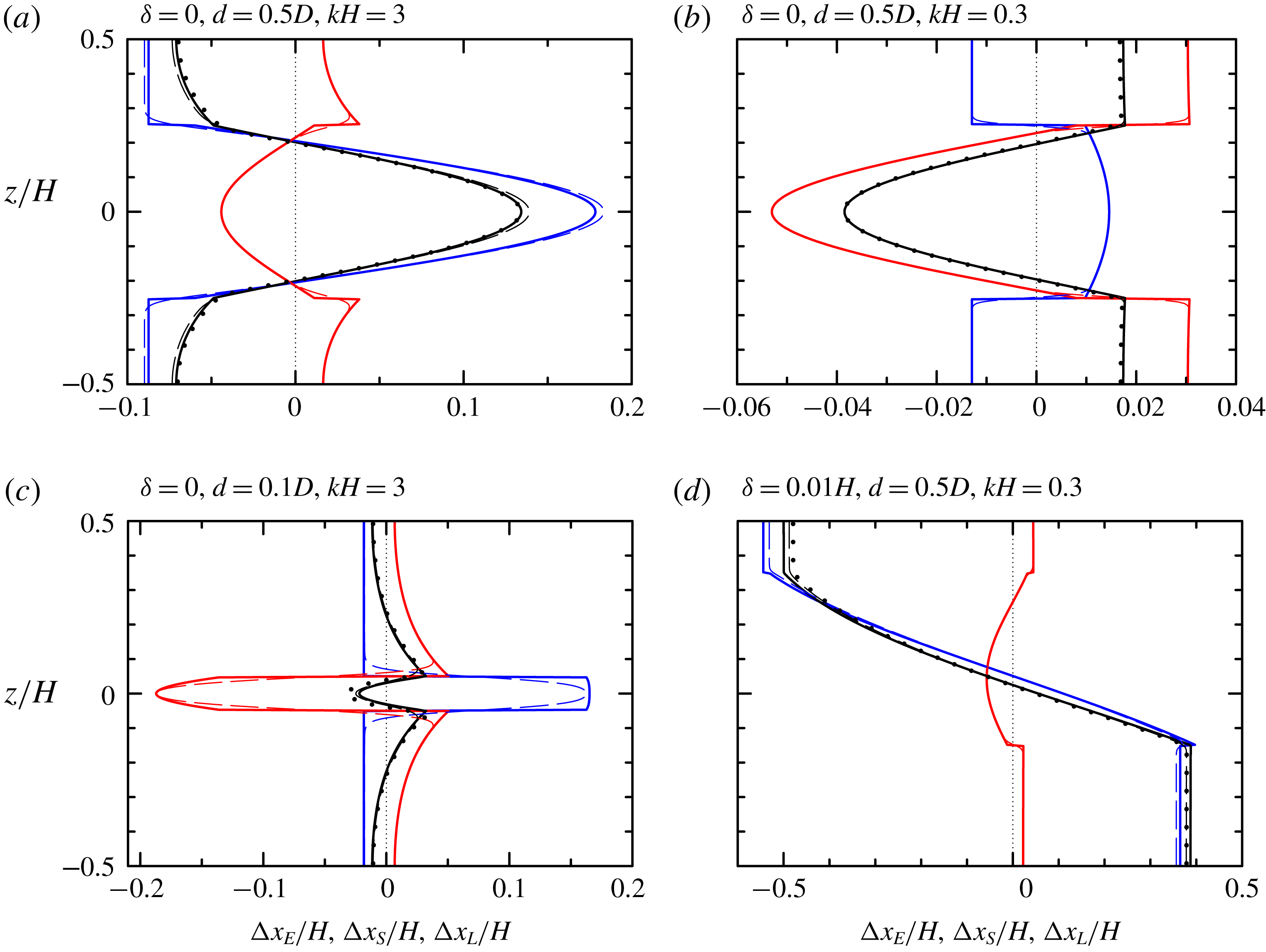
5.3 Exponential stratification
Finally, we consider the induced flow and Lagrangian displacements associated with an exponentially decreasing
 $N^{2}$
profile (4.46), more representative of oceanic stratification. Snapshots of the full horizontal velocity, including that associated with waves in the wavepacket, and the Fourier-filtered horizontal velocity are shown in figure 12. In this case with the stratification having e-folding depth
 $\unicode[STIX]{x1D70E}_{e}=0.1H$
and the waves having
 $kH=0.3$
, the induced flow is comparable to if not larger than the flow due to the waves themselves even though the wave amplitude is
 $a_{0}=0.01H$
. Apparently, the result of Doppler-shifting by the induced flow has affected the dispersion of the waves in the wavepacket as evident from the uneven spacing of crests.
From a numerical simulation having exponential stratification with e-folding scale
 $\unicode[STIX]{x1D70E}_{e}=0.1H$
and a wavepacket with
 $a_{0}=0.01H$
,
 $kH=0.3$
and
 $\unicode[STIX]{x1D70E}=50H$
, snapshots at
 $N_{0}t=3000$
of (a) the full horizontal velocity field associated with both the waves and their induced Eulerian flow and (b) the Fourier-filtered horizontal flow showing the induced Eulerian flow alone as well as the filtered parcel displacements.

As in figure 11 but for two simulations with exponential stratification having e-folding depth (a)
 $\unicode[STIX]{x1D70E}_{e}=0.2H$
and (b)
 $0.1H$
. In (a) the Gaussian wavepacket is initialized with
 $kH=1$
and
 $\unicode[STIX]{x1D70E}=20H$
and in (b)
 $kH=0.3$
and
 $\unicode[STIX]{x1D70E}=50H$
, as in the simulation shown in figure 12. In both simulations
 $a_{0}=0.01H$
.

Profiles of the predicted displacements and those measured in simulations are shown in figure 13 for cases with
 $\unicode[STIX]{x1D70E}_{e}=0.2H$
and
 $kH=1$
and with
 $\unicode[STIX]{x1D70E}_{e}=0.1H$
and
 $kH=0.3$
. In both cases the Eulerian flow decreases monotonically from a positive value at depth to a negative value at the surface. Following from our insights derived from the asymmetric two-layer and the asymmetric top-hat cases, the more negative Eulerian flow near the top and the more positive Eulerian flow near the bottom is a manifestation of the inherent ‘asymmetry’ of the exponential profile with these flows being larger if the upper layer is ‘thinner’ and the relative horizontal wavenumber is smaller. In the case shown in figure 13(a), the displacements measured in the lee of the wavepacket exactly matches the predicted Lagrangian displacements. However, in the case of long waves in shallower stratification in figure 13(b), the induced Eulerian flow acts back upon the waves so that the Lagrangian displacement at the surface is smaller in magnitude than predicted. As in the work of Grimshaw (Reference Grimshaw1977), it is expected that a nonlinear Schrödinger equation or similar weakly nonlinear model could be formulated to predict the observed displacements. However, the development and application of such a theory lies beyond the scope of this work.
6 Conclusions
We have derived general formulae for the Eulerian induced flow and the Stokes drift generated by horizontally modulated, vertically confined (or guided) internal wavepackets in a two-dimensional, Boussinesq fluid with arbitrary stable stratification. The predictions are validated by numerical simulations through comparing velocity and net displacement profiles. To gain insight into the connection between flows induced by interfacial waves and internal waves in continuous stratification, analytic solutions were found for the Stokes drift and Eulerian flow induced by waves in a two-layer fluid and in top-hat and exponential stratification.
In a symmetric two-layer fluid, the Stokes drift is positive everywhere with peak value at the interface, whereas the Eulerian flow is negative and uniform with depth for long groups. Combined, the net depth-integrated Lagrangian transport is zero in each layer, unless one layer is shallower than the other, in which case wave-averaged interface displaces into that layer making the Eulerian flow in that layer more negative and the Eulerian flow in the opposite layer more positive by the same amount. The depth-integrated flow across the whole fluid remains zero. By contrast, in continuous stratification the depth-integrated transport due to the Stokes drift and Eulerian flow are each zero. As the depth of the stratified layer in symmetric top-hat stratification becomes small, approaching the case of waves on a thin interface, the Stokes drift and the induced Eulerian flow in the uniform-density top and bottom layers approaches those predicted for interfacial waves in a two-layer fluid. However, the velocities within the stratified layer become larger as the interface becomes thinner. This is a consequence of the requirement that the vertically integrated Stokes drift and induced Eulerian flows each must be zero for waves in continuously stratified fluid. Because the velocities in the top and bottom layers have the same sign, the velocity in the stratified layer has opposite sign and must integrate over the small interface thickness to be equal and opposite to the integral of the velocities in the unstratified layers. While the mode-1 waves are sinuous, the corresponding Stokes drift and Eulerian velocities have a varicose vertical structure which can only exist in continuously stratified fluid, not in a two-layer fluid.
Both cases with top-hat and exponential stratification exhibit spikes in the induced Eulerian flow at finite horizontal wavenumber, and these can be attributed to resonances which occur when the vertical structure of the induced Eulerian flow corresponds to a mode moving with the same horizontal speed as the group velocity of the wavepacket, as noted originally by McIntyre (Reference McIntyre1973) for the case of uniform stratification. Importantly, while not possible with uniform stratification, another near resonance is apparent for wavepackets containing small horizontal wavenumber waves in vertically asymmetric stratification: the Eulerian induced flow is found to vary as the inverse square of the horizontal wavenumber. For asymmetric two-layer interfacial waves, it is manifest as the effect of the displacement of the wave-averaged interface into the shallower layer, enhancing in magnitude the negative Eulerian flow in that layer. For relatively long waves in exponential stratification, this ‘infrared catastrophe’ is dominant and causes large negative Eulerian flows in the ‘shallower’ region near the surface.
While this idealized study has generally examined the problem of transport by internal waves, the most obvious eventual application of this work is to understand transport by oceanic internal modes such as those generated by tidal flow over submerged ridges that emanate in the far field primarily as mode-1 internal tides (e.g. Martin, Rudnick & Pinkel Reference Martin, Rudnick and Pinkel2006). We have introduced a step in this direction by demonstrating that our model correctly predicts the Stokes drift and Eulerian induced flows for vertically confined internal waves in stratification that decreases exponentially with depth. Consistent with the analytic models, this study shows that both these flows contribute to the net Lagrangian transport. However, the infrared catastrophe associated with long-wave resonance suggests that the induced Eulerian flow should dominate and may even be so large as to influence the evolution of the waves themselves.
Away from resonance, the combined action of dispersion and nonlinearity not included herein will cause the packet to change shape slowly, as might be captured to leading order by a nonlinear Schrödinger equation (Grimshaw Reference Grimshaw1977, Reference Grimshaw1981; Liu & Benney Reference Liu and Benney1981). When the change is slow (away from resonance), the change in the net Lagrangian displacement will likely be small. At resonance, when infinite mean flows are predicted by second-order theory, the nonlinear Schrödinger equation breaks down and a system has to be formulated in which there is energy transfer between the linear waves and the mean flow as done by Koop & Redekopp (Reference Koop and Redekopp1981). The problem can no longer simply be thought of as steady in the reference frame of the packet. As the bound mean flow is a solution to the linear dispersion equation itself, we can superimpose an arbitrary mean flow as a free wave and the problem becomes dependent on initial conditions and needs to be conceptually redefined. Close to resonance, it will take very long for such an arbitrary mean flow to separate from the packet and its bound mean flow.
Future work aims to explore transport and long-wave resonance in more realistic detail through including the effects of background rotation (see recent work by Wagner & Young (Reference Wagner and Young2016) and Thomas, Bühler & Shafer Smith (Reference Thomas, Bühler and Shafer Smith2018)) and allowing for the wavepacket to have finite spanwise extent.
Acknowledgements
This research was performed in part through funding from the Natural Sciences and Engineering Research Council (NSERC) of Canada. T.S.v.d.B. was partially supported by the Faculty of Science at the University of Alberta through its Visiting Fellowship program and by a Royal Academy of Engineering Research Fellowship. The authors wish to thank P. Lelong and J. Early for their insights into the Stokes drift for internal modes.
Appendix A. Nonlinear forcing
From table 1, we can readily evaluate the following products occurring in the nonlinear forcing term
 ${\mathcal{N}}$
:
 $$\begin{eqnarray}\displaystyle & \displaystyle \overline{u^{(1)}\unicode[STIX]{x1D701}^{(1)}}=-{\displaystyle \frac{1}{4}}N^{2}|A_{0}|^{2}{\displaystyle \frac{\text{d}\hat{\unicode[STIX]{x1D702}}_{0}^{2}}{\text{d}z}}, & \displaystyle\end{eqnarray}$$
 $$\begin{eqnarray}\displaystyle & \displaystyle \overline{w^{(1)}\unicode[STIX]{x1D701}^{(1)}}=-{\textstyle \frac{1}{4}}N^{2}\left(1-2\unicode[STIX]{x1D712}\right)\unicode[STIX]{x1D700}\unicode[STIX]{x2202}_{X}|A_{0}|^{2}\hat{\unicode[STIX]{x1D702}}_{0}^{2}, & \displaystyle\end{eqnarray}$$
 $$\begin{eqnarray}\displaystyle & \displaystyle \overline{u^{(1)}b^{(1)}}=-{\displaystyle \frac{1}{4}}N^{2}c_{p}|A_{0}|^{2}{\displaystyle \frac{\text{d}\hat{\unicode[STIX]{x1D702}}_{0}^{2}}{\text{d}z}}, & \displaystyle\end{eqnarray}$$
 $$\begin{eqnarray}\displaystyle & \displaystyle \overline{w^{(1)}b^{(1)}}=+{\textstyle \frac{1}{4}}N^{2}c_{p}\unicode[STIX]{x1D712}\unicode[STIX]{x1D700}\unicode[STIX]{x2202}_{X}|A_{0}|^{2}\hat{\unicode[STIX]{x1D702}}_{0}^{2}, & \displaystyle\end{eqnarray}$$
where we have only given the leading-order contributions to the mean flow at second order in amplitude.
Appendix B. Vertical structure of vertical displacement at
$O(\unicode[STIX]{x1D6FC}\unicode[STIX]{x1D700})$

In addition to its forcing equation (3.5) and the no normal-flow boundary conditions
 $w(z=\pm D)=0$
, which imposes
 $\hat{\unicode[STIX]{x1D702}}_{1}(z=\pm D)=0$
, the
 $O(\unicode[STIX]{x1D6FC}\unicode[STIX]{x1D700})$
vertical structure function
 $\hat{\unicode[STIX]{x1D702}}_{1}$
must satisfy the relevant matching conditions at the ‘interface’. The kinematic condition requires that
 $\hat{\unicode[STIX]{x1D702}}_{1}$
is continuous across the interface in all three cases, but the dynamic boundary condition is different in each case.
B.1 Two-layer fluid: interfacial waves
Where
 $N^{2}(z)=0$
the forcing equation (3.5) and the no normal-flow boundary conditions
 $w(z=\pm D)=0$
allow a (continuous) solution of the form
 $$\begin{eqnarray}\hat{\unicode[STIX]{x1D702}}_{1,\pm }(z)=a_{0,\pm }\sinh (k(D\mp z))+a_{1,\pm }k(D\mp z)\cosh (k(D\mp z)),\end{eqnarray}$$
where the first term corresponds to the homogeneous solution
 $\hat{\unicode[STIX]{x1D702}}_{0}$
, and (3.5) requires in particular that
 $a_{1,\pm }=-1/\sinh kD_{\pm }$
with no restrictions on the homogeneous solution and thus
 $a_{0,\pm }$
. Equality of linearized total pressures at the interface,
 $p_{\text{tot},+}^{(1)}(z=\unicode[STIX]{x1D6FF}+\unicode[STIX]{x1D702}_{I})=p_{+}^{(1)}(z=\unicode[STIX]{x1D6FF})-\unicode[STIX]{x1D70C}_{+}g~\unicode[STIX]{x1D702}_{I}^{(1)}=p_{\text{tot},-}^{(1)}(z=\unicode[STIX]{x1D6FF}+\unicode[STIX]{x1D702}_{I})=p_{-}^{(1)}(z=\unicode[STIX]{x1D6FF})-\unicode[STIX]{x1D70C}_{-}g~\unicode[STIX]{x1D702}_{I}^{(1)}$
, gives the linear matching condition
 $$\begin{eqnarray}{\displaystyle \frac{\unicode[STIX]{x0394}p^{(1)}}{\unicode[STIX]{x1D70C}_{ref}}}\equiv {\displaystyle \frac{p_{+}^{(1)}-p_{-}^{(1)}}{\unicode[STIX]{x1D70C}_{ref}}}=-g^{\prime }\unicode[STIX]{x1D702}_{I}^{(1)}\quad \text{for }z=\unicode[STIX]{x1D6FF},\end{eqnarray}$$
which becomes at
 $O(\unicode[STIX]{x1D6FC}\unicode[STIX]{x1D700})$
using table 1 and the dispersion relationship (4.6)
 $$\begin{eqnarray}\hat{\unicode[STIX]{x1D702}}_{1,+}^{\prime }-\hat{\unicode[STIX]{x1D702}}_{1,-}^{\prime }+2(1-\unicode[STIX]{x1D712})\left(\hat{\unicode[STIX]{x1D702}}_{0,+}^{\prime }-\hat{\unicode[STIX]{x1D702}}_{0,-}^{\prime }\right)=-{\displaystyle \frac{k}{\tanh kD_{+}+\tanh kD_{-}}}\hat{\unicode[STIX]{x1D702}}_{1}\quad \text{for }z=\unicode[STIX]{x1D6FF}.\end{eqnarray}$$
The constant
 $a_{0,\pm }$
can be freely chosen (cf. homogeneous solution) and we set
 $a_{0,\pm }=0$
.
B.2 Symmetric top-hat stratification
The forcing equation (3.5) and the no-flow boundary conditions
 $w(z=\pm D)=0$
allow a (continuous) solution of the form
 $$\begin{eqnarray}\hat{\unicode[STIX]{x1D702}}_{1}=\left\{\begin{array}{@{}ll@{}}a_{0}\sinh k(D-z)+a_{1}k(D-z)\cosh (k(D-z)) & d<z\leqslant D,\\ a_{2}\cos \unicode[STIX]{x1D6FE}z+a_{3}\unicode[STIX]{x1D6FE}z\sin \unicode[STIX]{x1D6FE}z & |z|\leqslant d,\\ a_{0}\sinh k(D+z)+a_{1}k(D+z)\cosh \left(k(D+z)\right) & -d>z\geqslant -D,\end{array}\right.\end{eqnarray}$$
where we have 4 coefficients still be determined. Having invoked symmetry, we focus on the ‘interface’ between the top unstratified layer and the stratified layer. From the forcing equation (3.5) in the outer layer and inner layer, we obtain
 $a_{1}=-\!\cos \unicode[STIX]{x1D6FE}d/\sinh \,k\unicode[STIX]{x1D6E5}$
and
 $a_{3}=1+\unicode[STIX]{x1D712}/(\unicode[STIX]{x1D714}^{2}/N^{2}-1)$
, respectively. From the kinematic condition, we require that
 $\hat{\unicode[STIX]{x1D702}}_{1}$
is continuous across the interface at
 $z=d$
. For top-hat stratification, the hydrostatic pressure does not make a contribution to the linear dynamic matching condition, and we simply require that the pressure is continuous across the interface and thus so is
 $\hat{\unicode[STIX]{x1D702}}_{1}^{\prime }$
. We can solve these two conditions simultaneously to give
 $$\begin{eqnarray}a_{0}={\displaystyle \frac{\cos \unicode[STIX]{x1D6FE}d}{\sinh k\unicode[STIX]{x1D6E5}}}\left(1+{\displaystyle \frac{2k\unicode[STIX]{x1D6E5}}{\sinh 2k\unicode[STIX]{x1D6E5}}}\right),\quad a_{2}=\left(1+\displaystyle {\displaystyle \frac{\unicode[STIX]{x1D6FE}d}{\tan \unicode[STIX]{x1D6FE}d}}\right){\displaystyle \frac{1-\displaystyle {\displaystyle \frac{2k\unicode[STIX]{x1D6E5}}{\sinh 2k\unicode[STIX]{x1D6E5}}}}{1+\displaystyle {\displaystyle \frac{2\unicode[STIX]{x1D6FE}d}{\sin 2\unicode[STIX]{x1D6FE}d}}}},\end{eqnarray}$$
where we have used
 $$\begin{eqnarray}\unicode[STIX]{x1D712}\equiv {\displaystyle \frac{c_{g}}{c_{p}}}={\displaystyle \frac{\unicode[STIX]{x1D6FE}^{2}}{\unicode[STIX]{x1D6FE}^{2}+k^{2}}}\left(1-{\displaystyle \frac{1-\displaystyle {\displaystyle \frac{2k\unicode[STIX]{x1D6E5}}{\sinh 2k\unicode[STIX]{x1D6E5}}}}{1+\displaystyle {\displaystyle \frac{2\unicode[STIX]{x1D6FE}d}{\sin 2\unicode[STIX]{x1D6FE}d}}}}\right).\end{eqnarray}$$
Appendix C. Details of numerical simulations
For numerical stability, Laplacian diffusion is applied to the basic-state fields, but only to disturbances with horizontal wavenumbers higher than four times that of the horizontal wavenumber of waves in the wavepacket. The Reynolds number, based on the maximum buoyancy frequency
 $N_{0}$
and domain depth
 $H$
is
 $Re=(N_{0}H^{2})/\unicode[STIX]{x1D708}=10^{5}$
. The Prandtl number is
 $1$
. Although the Reynolds number is much smaller than that for typical geophysical flows and the Prandtl number is smaller than that associated with relative heat (or salt) diffusion, these diffusive processes negligibly affect the dynamics, especially as the selective application of diffusion means that neither the waves nor the induced flow experience diffusion.
In practice, we find the predicted Eulerian flow is well reproduced in simulations run at relatively low resolution and coarse time steps. However, for quantitative accuracy the simulations reported upon with uniform and exponential stratification had a vertical resolution of
 $H/128$
and a horizontal resolution of
 $k^{-1}/16$
with time steps taken at intervals of
 $0.01N_{0}^{-1}$
. In top-hat-like stratification the vertical resolution was taken to be
 $H/256\simeq 0.004H$
in order to resolve the transitions from zero to strong stratification over a distance
 $\unicode[STIX]{x1D70E}_{d}\simeq 0.02H$
. In all cases, for accurate determination of the Lagrangian flow, for which parcel displacements associated with the Stokes drift as well as Eulerian flow needed to be resolved, the simulations required shorter time steps of
 $0.001N_{0}^{-1}$
. The simulations were run for a duration allowing the wavepacket to propagate a distance of at least
 $6\unicode[STIX]{x1D70E}$
so that the vertical profile of the Lagrangian displacement could be extracted sufficiently ahead of the wavepacket’s initial position and sufficiently far behind its final position – a distance of approximately
 $3\unicode[STIX]{x1D70E}$
. Depending upon the stratification and wavenumber, which set the horizontal group velocity of the wavepacket, simulations took between two and six days to run on a Mac desktop computer with a 2.2 GHz Intel Core i7 processor.



