


Introduction
Many landforms left by continental ice sheets owe their origin to thermal conditions at the glacier bed. Thrust features probably formed in places where the glacier margin was frozen to the substrate but pressure-melting conditions existed a few kilometers up-glacier (Reference Moran, Clayton, Hooke and FentonMoran and others, 1980). Further inland, at down-flow transitions from a frozen to a thawed bed, higher areas may have remained frozen while lower ones were at the pressure-melting point. Preserved in some of these higher areas are relict periglacial landforms that developed during the last interstadial, such as patterned ground (Reference KlemanKleman and Borgström, 1994) and tors (Reference Kleman and HattestrandKleman and Hättestrand, 1999). Longitudinal compression on the stoss sides of such cold patches may result in stacked transverse moraines; extension in their lee leaves abrupt scarps (Reference KlemanKleman and Börgstrom, 1994). Drumlins may also be nucleated by such frozen islands (e.g. Reference Patterson and HookePatterson and Hooke, 1995, p.30). At boundaries between zones of thawed and frozen bed, ribbed moraine may form by pull-apart of a once continuous drift sheet (Hättestrand and Reference Kleman and HattestrandKleman, 1999). Finally, the subglacial thermal regime may influence esker formation.
Numerical modeling provides a powerful tool for testing such hypotheses. If the model suggests that there is no possibility of the presumed bed conditions having existed at the appropriate time, alternative explanations for the landforms must be sought. Conversely, to the extent that such hypotheses for the origin of the landforms can be independently verified, the distribution of the features can be used to tune numerical models. Our goal herein is to take a first step towards both of these goals. We tuned the model so that the margin of the model glacier was in certain locations at times that are consistent with field evidence. We then tested it by comparing the predicted basal and mean annual marginal temperatures with those suggested by field data. Finally, we asked what the basal conditions were, how they evolved through time and how they may have contributed to esker development.
The Model
We used the University of Maine Ice Sheet Model, a mapplane vertically integrated finite-element model developed by Fastook (Reference Fastook and ChapmanFastook and Chapman, 1989;Reference FastookFastook, 1990; Reference Fastook and PrenticeFastook and Prentice, 1994;Reference JohnsonJohnson, 2002;Reference Johnson and FastookJohnson and Fastook, 2002). The model can simulate the advance and retreat of the Laurentide and other ice sheets over several glacial cycles. Run in this mode, its output is consistent with that of 15 other ice-sheet models (Reference Huybrechts, Payne and Intercomparison GroupHuybrechts and others, 1996;Reference PaynePayne and others, 2000). After running the full model for a complete glacial cycle with a coarse grid spacing, one can zoom in on successively smaller areas and run it with much finer grid spacings and a higher time resolution. The earlier solution provides time-dependent boundary conditions for the next (see Appendix A). In our case, we focused on the state of Maine during the period from the Last Glacial Maximum (LGM) to some time before the Younger Dryas.
Climate
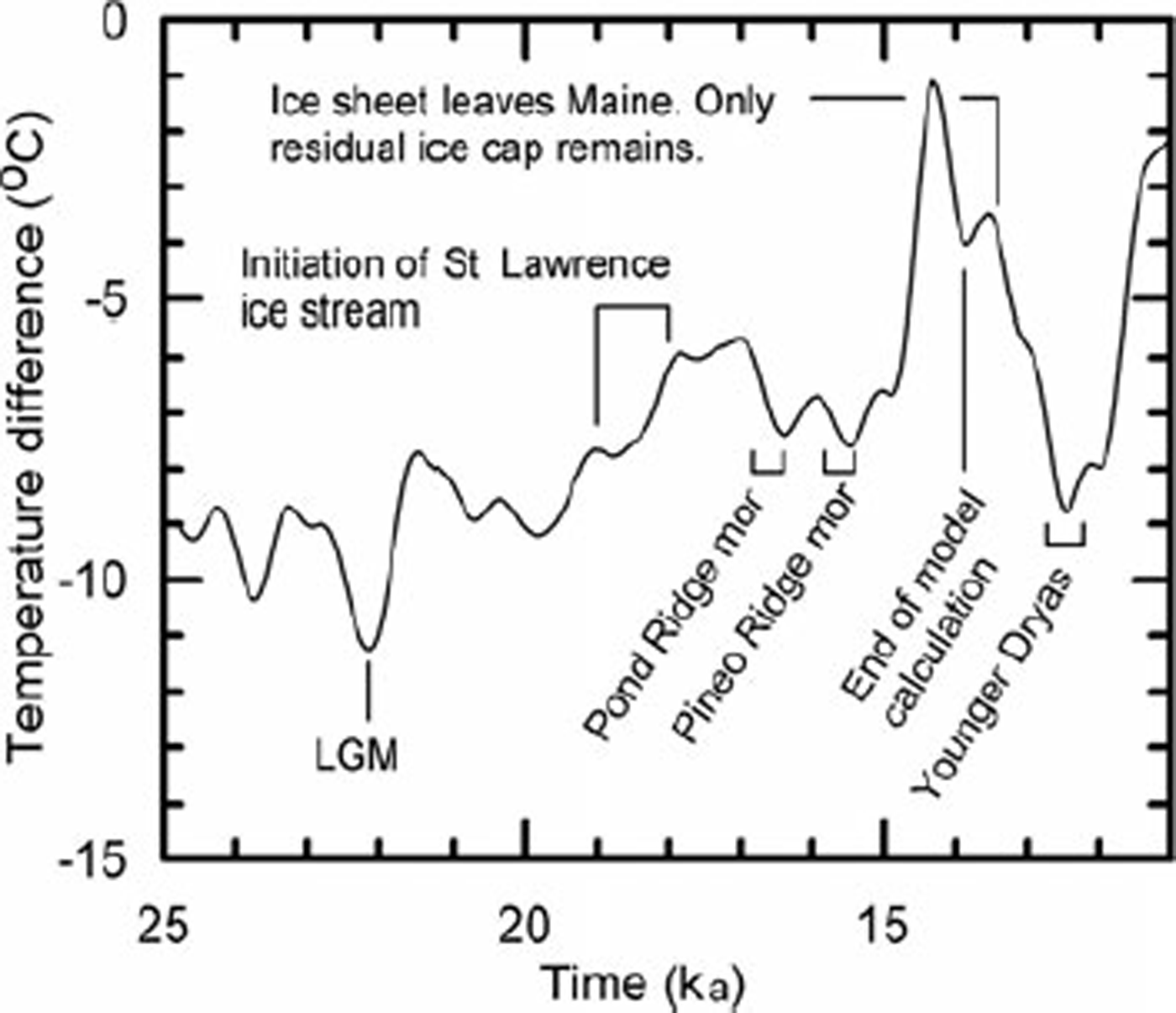
As is the case with real ice sheets, the model ice sheet is driven by climate. The δ18O record from the Greenland Icecore Project (GRIP) ice core (Reference DansgaardDansgaard and others, 1993;Reference TaylorTaylor and others, 1993) is used to estimate the temperature in the past at the GRIP drill site (Fig. 1) (Reference Johnsen, Dahl-Jensen and DansgaardJohnsen and others, 1995). At an arbitrary reference point in Maine, the present mean annual temperature is warmer than that at GRIP by an amount ΔT. We refer to this difference as the offset. To generate a proxy record of the temperature distribution over the modeled region in the past, we first add the offset to the GRIP record. Outwards from the reference point we then use present latitude and elevation lapse rates to adjust for geographic location and, in the case of elevation, for the presence of the ice sheet.
From the temperature, we obtain the saturation vapor pressure. Snowfall is then calculated from a correlation between it and saturation vapor pressure (Reference Fastook and PrenticeFastook and Prentice, 1994). Melt rates are based on a positive-degreeday treatment with allowance for daily temperature cycling across 0°C. In the ablation area, this simple parameterization yields a negative specific mass balance that becomes less negative with increasing elevation. Above the equilibrium line, it yields a positive balance that peaks at the elevation where daily temperature cycles no longer rise above 0°C, and then declines to values typical of a polar plateau at higher elevations. The lapse rates and initial value of the offset are adjusted to yield current mean annual temperatures, as closely as possible (given the limitation of a linear latitudinal lapse rate), within the domain of interest. The latitudinal pole is placed in North Greenland to accommodate the asymmetry of Northern Hemisphere ice sheets.
Finally, the resulting climate is tuned so that, in our case, the ice-sheet margin coincides reasonably well with certain observed marginal positions. Tuning consists of making small changes in the magnitude of the fluctuations in Figure 1 and in the offset.
Ice temperature
Temperatures within and at the base of the ice sheet are calculated based on the mean annual surface temperature, advective effects of ice flow (see Appendix B), strain heating and geothermal flux. The feedback between temperature and ice strain rate is achieved through an iterative process.
In the ablation area, the near-surface ice temperature is likely to be a degree or so warmer than the mean annual atmospheric temperature. This is because the winter snow cover insulates the ice from the deepest winter cold, and percolating meltwater warms the ice before the snow cover disappears in the spring (Reference Hooke and GouldHooke and others, 1983). We refer to this difference as Δθ. Above the equilibrium line, percolating meltwater can penetrate into permeable firn, releasing the heat of fusion deeper in the glacier. On Barnes Ice Cap, where equilibrium-line temperatures (∼−10°C) and June snow depths (∼0.5mw.e.) are comparable to those predicted by our model for the Laurentide in Maine, these processes result in a Δθ of ∼2 K in the ablation area and ∼4 K above the equilibrium line. Δθ decreases rapidly with decreasing temperature (equivalent to increasing elevation). Our model does not take Aθ into consideration, so our nearsurface ice temperatures are likely to be too cold in the ablation area and lower part of the accumulation area. Thus, our basal temperature gradients are probably slightly too high, and melt rates too low.
The model also ignores transient changes in heat flux at the ice/bed interface resulting from changes in interface temperature. Between ∼33 and 29.5 ka (calibrated or calendar years before present;Reference Bronk RamseyBronk Ramsey, 1995, Reference Bronk Ramsey1998) as the ice was making its way into Maine and southwards to the edge of the continental shelf, our model suggests that the mean annual temperature at the margin was ∼−3°C. Thus, the glacier was presumably advancing over thin permafrost. The model predicts that the ice/bed interface would have been near to or at the pressure-melting temperature nearly everywhere in Maine except very close to the margin. Thus, the temperature at the interface would have had to increase ∼3°C as the ice advanced over it. We are interested, in particular, in basal conditions after 16.1 ka, so the temperature gradient in the substrate would have had ∼13 kyr to adjust. Calculations using both a theoretical solution by Reference Carslaw and JaegerCarslaw and Jaeger (1959, p. 62–63) and a numerical model suggest that the heat flow reaching the interface by that time would have been 99.9% of the long-term average value. Thus, a correction for this transient effect is not necessary.
Temperature record from GRIP in Greenland, used to drive model. The record is expressed in terms of the difference in temperature between the present and the past at GRIP.
Sliding
Because the ice surface slope is low and the bed is generally at the pressure-melting point in our model, over 90% of the surface velocity is a result of sliding. The sliding law used is

based on that of Reference WeertmanWeertman (1957b, Reference Weertman1964) modified to incorporate the effect of water at the base of the ice sheet. Here us ρ·, g, h, α and w are the sliding speed, density of ice, acceleration due to gravity, ice thickness, surface slope, and amount of available water (including pore-water in the subglacial sediment), respectively, and Cs is Weertman’s sliding coefficient. Cs depends on parameters including bed roughness, solute content in the basal ice and rock-to-rock friction, none of which can be known well enough to parameterize independently.
The effect of water on us is widely recognized but, as yet, poorly understood. It appears that us is dependent both on water pressure, Pw , and on w (Reference Kamb, Engelhardt, Fahnestock, Humphrey and MeierKamb and others, 1994). Beneath ice sheets, Pw is expected to be close to the overburden pressure (Röthlisberger, 1972;Reference ShreveShreve, 1972). Thus, variations in w may have more effect on us than variations in Pw .
The basal melt rate is used to calculate w. Longitudinal flow of water along the bed or input of water from the surface are not included. However, Cs and the exponents p and q are chosen to yield velocities that agree with those of measured ice streams and that are consistent with results from a more sophisticated (but computationally more timeconsuming) model module that includes longitudinal water flow (Johnson, 2006).
That water might reach the bed of a polar glacier by propagation of water-filled crevasses was predicted theoretically by Reference GlenGlen (1954) and Reference WeertmanWeertman (1973), but only recently verified by observations (Reference Zwally, Abdalati, Herring, Larson and SabaZwally and others, 2002; Reference Boon and SharpBoon and Sharp, 2003). As we do not include this water source in calculating w, we may not adequately capture any down-glacier increase in us that occurs where water from the surface first gains access to the bed. We think, however, that this effect is largely smoothed over by tuning, and that the uncertainty introduced is small compared with that resulting from a lack of a rigorous theoretical basis for relating us to Pw and w. Furthermore, sensitivity tests described below suggest that the uncertainty in us has little effect on our basic conclusions.
Calving
To approximate ice loss by calving at the grounding line, the longitudinal strain rate  is estimated from

where ρw
is the density of sea water and the ice is assumed to be close to flotation (Reference WeertmanWeertman, 1957a). Making the approximation that the flow is two-dimensional so 
 the thinning rate is
 This thinning is added to the (negative) mass balance at the margin. Subsequent comparison with a Reference Brown and MeierBrown and others (1982) form of calving law showed little difference between the two approaches. While both accelerated ice loss in the Gulf of Maine, neither resulted in a calving bay migrating up the St Lawrence lowland.
Isostatic adjustment
The model takes isostatic adjustment into consideration, using beam theory to distribute the load of the ice sheet and including a 1/e relaxation time of 3 kyr.
Limitations
The model cannot simulate development of ice streams. The implications of this are discussed in the following section. In addition, the procedure for estimating longitudinal advection of heat is still rather crude. The consequences of this are unknown.
Tuning
In tuning, we tried to adjust the model so that the margin was just offshore of Cape Cod at the LGM (∼22.0ka), just inland of the present coast in eastern Maine at ∼16.1 ka and in north-central Maine at ∼14 ka. As margin positions were changing rapidly at this time, and are better defined than their ages, we opted to try to match margin positions and let age be a free variable. To achieve satisfactory fits, we increased the offset so the difference in temperature between Greenland and North America was slightly larger relative to today, and we reduced the magnitude of the fluctuations in Figure 1 by ∼10º%. Both are consistent with global climate models that suggest that, due to snow and sea-ice albedo effects, meridional temperature gradients were likely to have been larger during deglaciation than at present (e.g. Reference RindRind, 1998).
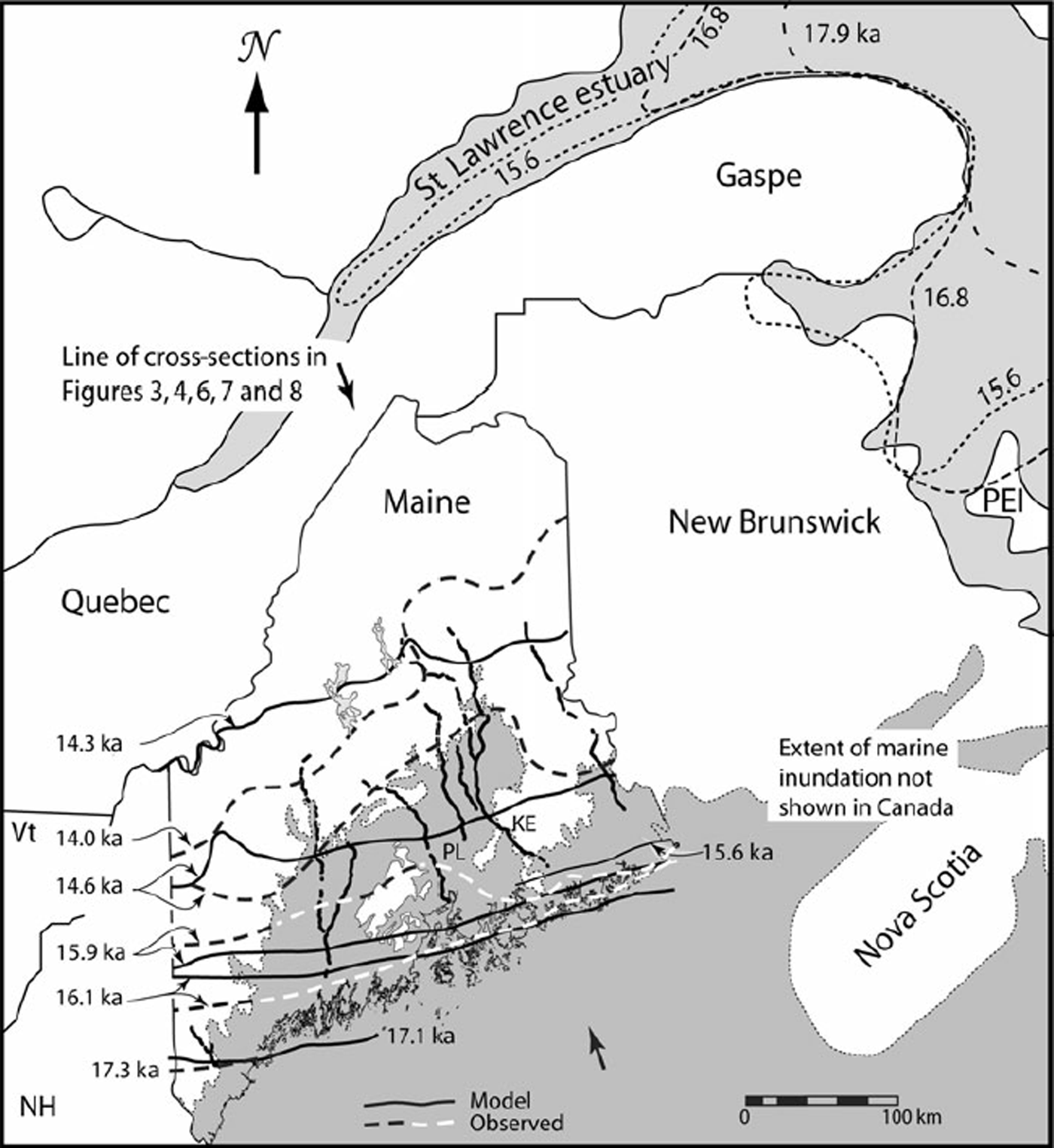
In Figure 2 we compare margin positions predicted by the tuned model with those based on field data and 14C dates (Reference Boon and SharpBorns and others, 2004). We will refer to the Borns and others positions as ‘observed’, recognizing that there is uncertainty in precise locations, in ages, and in temporal correlations.
In drawing their ice margin positions, Reference Boon and SharpBorns and others (2004) took into consideration evidence from striations, major topographic elements, end moraines, other ice contact deposits, and detailed local maps. Recognizing the uncertainties in the marine reservoir correction and those resulting from the radiocarbon plateau, and also noting that many dates are minimum estimates of the time of deglaciation, they gave precedence to field evidence where such evidence violated the 14C chronology. In addition, we note that moraines and other ice-marginal indicators are not common in Maine during the time period of interest.
At 17.1 ka, the margin of the model glacier coincides with that observed at 17.3 ka (Fig. 2). Our 16.1 ka margin is slightly too far south in eastern Maine, but our 15.9 ka margin is in good agreement with that observed. In western Maine, both fall between the corresponding observed positions. Our 15.6 ka margin is within 5 km of the mapped position of the 15.6 ka Pineo Ridge moraine in eastern Maine. Our 14.6 ka margin matches that observed in far eastern Maine, but does not show the substantial northward deviation around the Penobscot lowland (PL in Fig. 2) suggested by Reference Boon and SharpBorns and others (2004), and is too far north in western Maine. We harbor some doubts about the northern swing of the observed margin around the lowland, as the abrupt turn of the Katahdin esker (KE) to the east, out of the lowland and through a range of low mountains (Fig. 2), is not consistent with a calving bay in the lowland. Our 14.3 ka margin is south of the observed 14.0 ka margin in eastern Maine and north of it in western Maine. In summary, the model glacier appears to reach the coast 100–200 years too late and to retreat too fast in the west and, between 14.6 and 14.3 ka, too slowly in the east. Further tuning might have reduced some of the remaining discrepancies, but experience suggests that our basic conclusions would not be altered.
We attribute the discrepancy in the orientation of the 14.3 ka margin to the inability of our model to simulate the drawdown caused by an ice stream that is believed to have formed between 18 and 19 ka in the St Lawrence lowland to the north (Figs 1 and 2) (Reference Occhietti, Parent, Shilts and DionneOcchietti and others, 2001, p. 259). At ∼18.4 ka the ice shelf into which this ice stream flowed appears to have broken up, opening a calving bay in the mouth of the St Lawrence estuary. Over the next 3 kyr, this calving bay is thought to have migrated westward and then southwestward up the St Lawrence estuary (Fig. 2). The ice sheet in Maine may have begun to feel the effects of this drawdown as early as 18 ka (Reference Occhietti, Parent, Shilts and DionneOcchietti and others, 2001, fig. 2), but the apparent correlation of the Pineo Ridge moraine with the 15.6 ka cold event suggests that the margin in Maine did not react to the decrease in ice flux across the St Lawrence until later. In due course, however, there presumably would have been a progressive decrease, from east to west, in the flow of ice into Maine. This would have resulted in a more rapid retreat in the east. By 14 ka the residual ice in Maine is believed to have been completely cut off from the rest of the Laurentide ice sheet.
Tests of the Model
Margin temperatures at 16 ka
We next compare several estimates of the mean annual temperature at the glacier margin at 16 ka with those predicted by our model. Faunal species in the ice-proximal facies of the Presumpscot Formation suggest arctic to subarctic conditions, with sea temperatures of +1 to −2°C at this time. Oxygen and carbon isotope ratios in the same fauna suggest water of normal salinity with a temperature between 0 and +2°C (Reference Dorion, Balco, Kaplan, Kreutz and WrightDorion and others, 2001). To get a sense of the relation between these water temperatures and air temperatures in a modern glacial setting, we compared mean annual sea surface and air temperatures at 68° N off the west coast of Greenland (US National Oceanic and Atmospheric Adminsitration, http://ferret.pmel.noaa.gov/ NVODS/servlets/dataset?catitem=16133). The two were within a degree of each other, the air being slightly colder.
Location map of Maine (Vt = Vermont; NH = New Hampshire) showing observed (dashed lines) and modeled (solid lines) margins at various times. Also shown are the marine limit (in Maine only), major eskers and Reference Occhietti, Parent, Shilts and DionneOcchietti and others (2001) reconstructions of ice margins in the Gulf of St Lawrence and St Lawrence estuary. KE = Katahdin esker; PL = Penobscot lowland.
Geomorphic data are consistent with these temperatures. Glaciotectonic thrust features are common in LGM moraines on Cape Cod, Massachusetts (Reference OldaleOldale and O’Hara, 1984). Reference Moran, Clayton, Hooke and FentonMoran and others (1980) have argued that such features form where permafrost in the proglacial area extends a distance of 2–3 km under the ice margin so that the bed is frozen there. High pore-water pressures may then result in shear failure at the base of the permafrost. Other features characteristic of permafrost and presumably dating to a time shortly after the LGM are also found in outwash on Cape Cod (Reference OldaleOldale and O’Hara, 1984).
Similarly, Reference Stone and AshleyStone and Ashley (1992) and Reference Ashley and StoneAshley and others (1999) have found ice-wedge casts and pingo scars in the Connecticut River Valley, ∼150km north of the LGM ice margin. They also describe pollen and macrofossil assemblages from this area that are diagnostic of arctic to subarctic climate with subzero mean annual temperatures. Dates on some of these materials suggest that permafrost conditions persisted here until ∼15ka.
The southern edges of continuous, discontinuous and patchy permafrost in Canada presently roughly coincide with the −8, −4 and −1°C mean annual temperature isotherms, respectively (Reference BrownBrown, 1970, fig. 3). Thus, we can probably safely assume a mean annual temperature somewhere between 0 and –4°C at the ice margin in Maine at 16 ka.
For comparison, our model gives a mean annual icemarginal temperature of ∼–1°C at that time. We emphasize that we tuned the model to give this position at ∼16 ka, but did not tune it to this temperature; this is therefore an independent test of the model.
Basal temperatures
We mentioned earlier several landforms or landform assemblages that are believed to develop when an ice sheet is, at least locally, frozen to the bed. In our model ice sheet, there was only one small frozen area in western Maine at 22 ka, but more had developed by 18 ka and by 15.6 ka the whole northern quarter of the state was frozen (Fig. 3). Owing to the resolution of our model, we could not have detected a narrow frozen margin.
Of the landforms we mentioned, areas of relict periglacial landscape are not known from Maine and, based on our model, would not be expected as there were no areas that remained permanently frozen. However, scattered drumlins are found throughout southern Maine and there is an extensive area mapped as ribbed moraine in the lee of Mount Katahdin (MK in Fig. 3a) (Reference Thompson and BornsThompson and Borns, 1985). The drumlins could have been nucleated as the ice advanced, overriding permafrost, or by perturbations other than frozen patches. While we did not find frozen bed conditions in the area of ribbed moraine south of Mount Katahdin, the melt rate there at 18 ka was <1 mm a−1, so given the uncertainty in the model parameters, particularly in the geothermal flux and longitudinal advection of cold ice, freezing conditions there are well within our limits of uncertainty.
Maps of basal melt rate at (a) 22.0, (b) 18.0, (c) 15.6, and (d) 14.5 ka. Ice-sheet margin Is just south of either the 0 or 1 mm a−1 contour. Lakes shown are, from southwest to northeast, Sebago, Moosehead and Chesuncook. Rivers are the Kennebec (west) and Penobscot (east). MK = Mount Katahdin.

Moraines
It is particularly satisfying that the well-known pause in retreat at the coast at 15.6 ka, resulting in the Pineo Ridge moraine (e.g. Reference Dorion, Balco, Kaplan, Kreutz and WrightDorion and others, 2001), is reproduced well by our model. This pause is one of two, corresponding to two small cold reversals recorded in the Greenland ice core between 17 and 15 ka (Fig. 1). These pauses show up clearly in an animation of the ice-sheet margin on the computer screen. The earlier pause occurs between 16.5 and 16.3 ka just off the present coast and 24 km seaward of the Pond Ridge moraine, dated to 16.5 ka (Reference KaplanKaplan, 1999). The ages of these two moraines, although having a resolution of probably no better than ±200 years, both fall during the cooling phases of the cold reversals. This, rather than the period of maximum cooling, is the time when moraine building would be expected. Of course, we tuned the model to obtain an ice margin just inland from the coast at ∼16 ka. However, we did not tune the model to obtain morainebuilding pauses at these times and locations.
Results
Ice-sheet profiles
Profiles of the ice-sheet bed and surface along an approximate flowline are shown in Figure 4. At the LGM the model bed was depressed ∼250 m at the present coastline. By 14.25 ka, it had rebounded ∼50 m.
Cross-sections showing calculated ice-sheet surface and (isostatically depressed) bed topography at various times. Tick marks labeled E show locations of equilibrium lines. Equilibrium line for 14 ka profile is to the right of the diagram. Discrepancies between profiles, particularly along the bed, are a consequence of scaling elevations from computer-generated maps of the bed and surface topography with contour intervals of 75 and 250 m, respectively.

The surface profile of our model ice sheet steepens during retreat. Although contrary to popular conception, this is a logical consequence of an increase in temperature. When the temperature is above freezing, the model assumes that the ablation rate increases linearly with temperature (reaching ∼5 ma”‘ at the margin at 15.6 ka). In the model, an increase in temperature alone therefore simply increases the daily melt by the same amount everywhere in the ablation area. However, because the number of days with temperatures above 0°C is higher at lower elevations, the increase in annual ablation is significantly larger near the margin. For example, with a mean annual temperature at the margin of +4°C, a sinusoidal annual temperature cycle with a range of 12 K and a lapse rate of−0.006 K m−1, a 1 K increase in mean annual temperature results in an increase in the annual melt rate at the margin which is more than twice the increase at the elevation of the 15.6 ka equilibrium line. The slope of Bre¡ðamerkurjökull in Iceland increased in a similar fashion as it retreated between 1903 and 1998 (Reference Evans and TwiggEvans and Twigg, 2002, fig. 4).
Field evidence is sometimes interpreted as reflecting a decrease in marginal slope during retreat. Reference JahnsJahns (1953) and Reference KoteffKoteff (1974), for example, visualize a marginal zone of thin ‘stagnant’ ice with a low surface slope bordering active ice. Their marginal zone is only a few kilometers wide and may develop due to accumulation of a moraine cover with a consequent reduction in ablation rate. Although this ice is referred to as stagnant, ‘slowly moving’ would probably be more accurate. Development of such a zone cannot be simulated with our model, as the spatial scale is less than our ∼12 km grid spacing and we do not have an algorithm for debris content of basal ice.
Basal melt rate
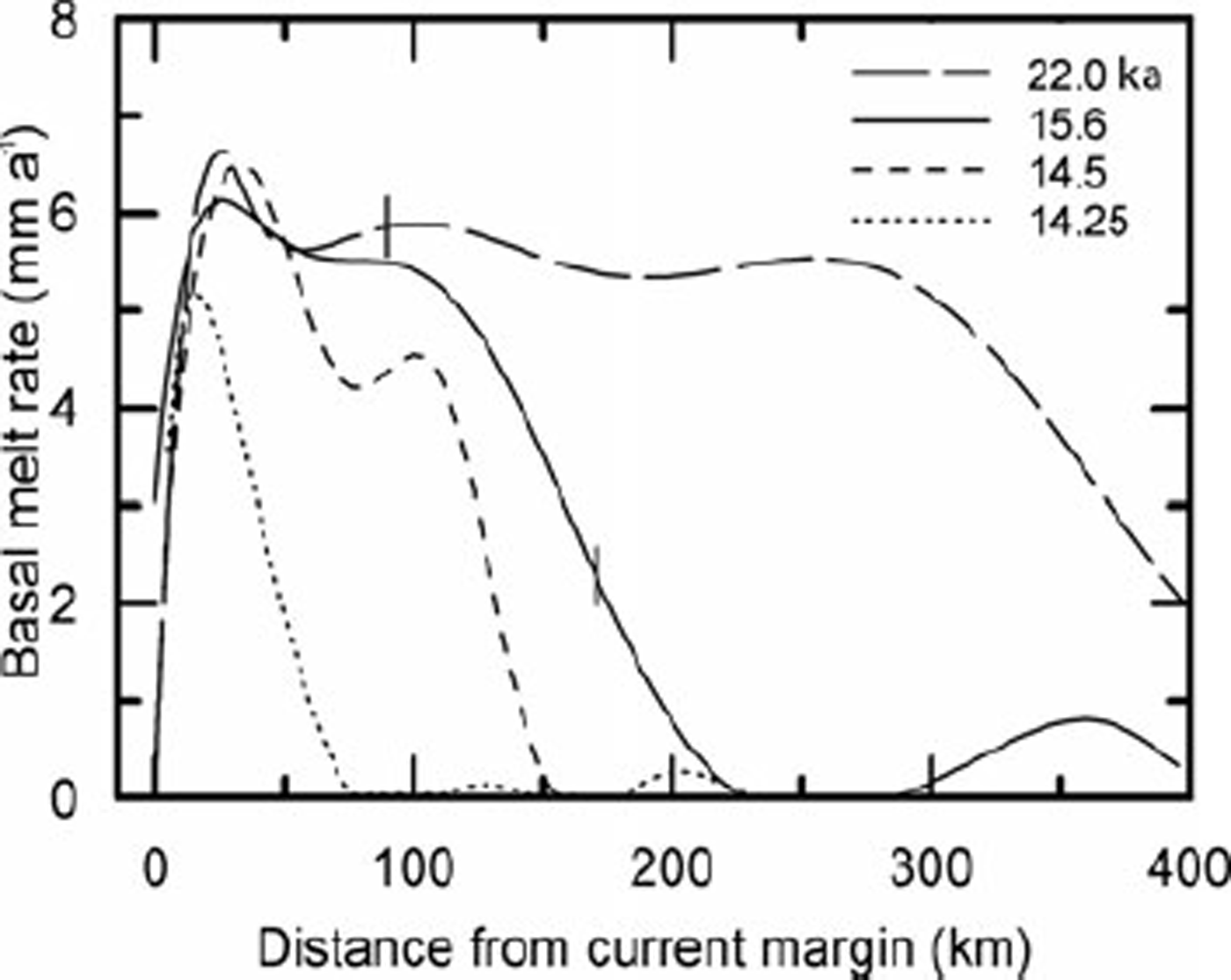
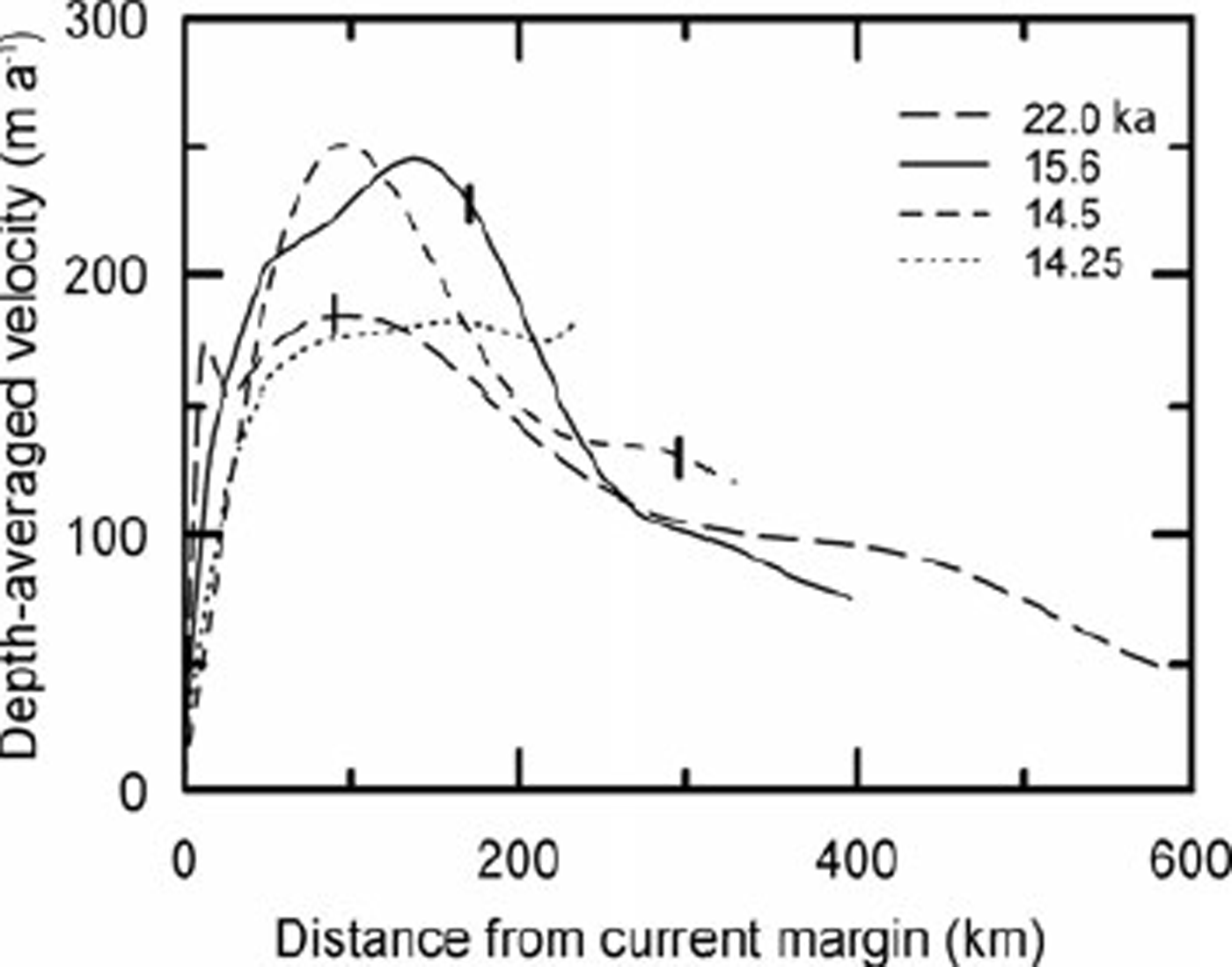
In nature, the basal melt rate m (Figs 3 and 5) is determined by the difference between: (1) the heat reaching the bed from the interior of the Earth (the geothermal flux) plus that generated at the bed by strain heating, and (2) the heat lost by conduction upwards into the ice. The heat produced at the ice/bed interface by strain heating is csτus where c s is a coefficient of proportionality, τ is the basal traction and us is the sliding velocity. The value of cs depends upon the effective strain rate, the bed slope and the bed roughness. csτus cannot be significantly greater than the potential energy lost as the center of mass of an ice column moves to lower elevations. On a horizontal bed, the potential energy lost as the center of mass of an ice column decreases in elevation is τus /2. On the adverse bed slopes that commonly result from isostatic depression of the crust, the decrease in potential energy is still less than this, and some of this energy is dissipated as heat through straining in the ice, including flow around irregularities on the bed. Thus, c s is generally significantly less than 1/2. In an ice stream, most of the potential energy lost is dissipated in side shear, so cs ≪ 1/2. In the model, we use cs = 0.1, but suspect that this may be a little low. We also assume that the geothermal flux is spatially uniform and τ turns out to be nearly uniform. Thus in the model, spatial variations in heat input are largely due to variations in u s (Fig. 6).
The calculated basal melt rate is 0 at the margin, but rises rapidly to 5–6 mm a−1 within a few kilometers (Figs 3 and 5). It then declines gradually for 150 km or so, before beginning a more precipitous decrease. Owing to the uncertainty in c s , these melt rates may be low.
Basal temperature gradient
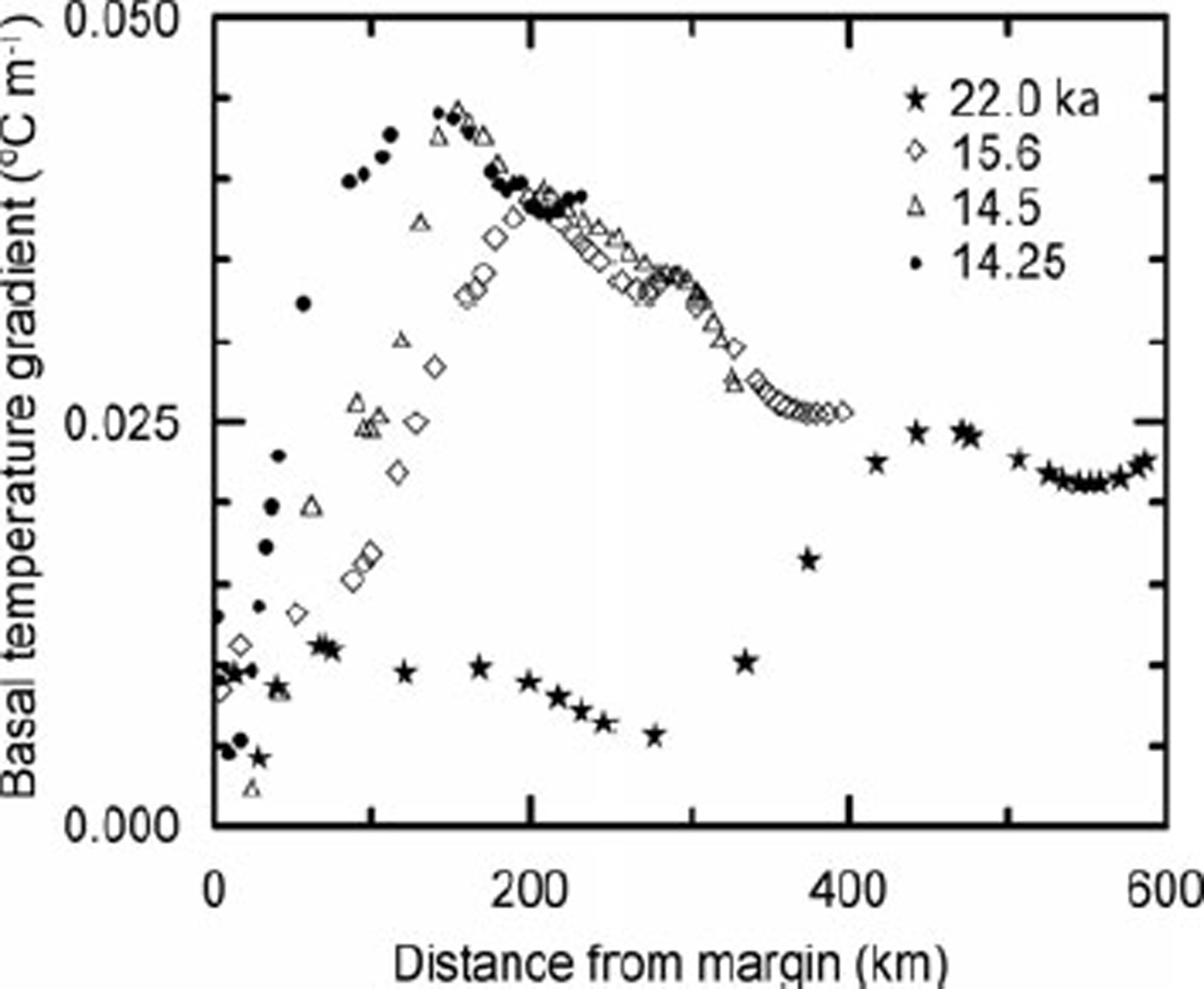
The rate at which heat is lost upward into the ice is closely proportional to the basal temperature gradient, ß o . When there is liquid water at the bed, this gradient is determined (both in nature and in the model) by the mean annual temperature at the glacier surface, conduction of heat in the ice, advection of heat by ice flow, strain heating, and transient changes associated with the changing climate. ß o is not output from the model, however. Thus, we calculated it from the difference between the energy input and that consumed by melting; it is plotted in Figure 7. ßo is largest where the vertical velocity is downward, moving cold ice toward the bed, and where there is appreciable strain heating at the ice/bed interface. Owing to the high sliding speed the vertical velocity is downward throughout the upper half of the ablation area.
Basal melt rate at various times as a function of distance from current margin. Tick marks show positions of equilibrium lines.
Depth-averaged velocity at various times as a function of distance from current margin. Tick marks show positions of equilibrium lines.
At distances greater than about 50 km from the glacier margin, ßo increases dramatically as the ice sheet begins to retreat. There is relatively little change in the spatial pattern of ß o between 15.6 and 14.25 ka; the pattern simply shifts northward with the ice margin. The rapid decline in ßo near the margin contributes to the peak in melt rate there (Fig. 5).
Sensitivity studies
The model parameters to which our results are most sensitive are c s , the geothermal flux and the enhancement factor in the ice flow law. The latter is the factor by which the ice flow rate is increased over that in pure laboratory ice with a random orientation of c axes. Flow of natural ice is commonly faster owing to development of crystal fabrics with preferred orientations and to the presence of impurities, among other things.
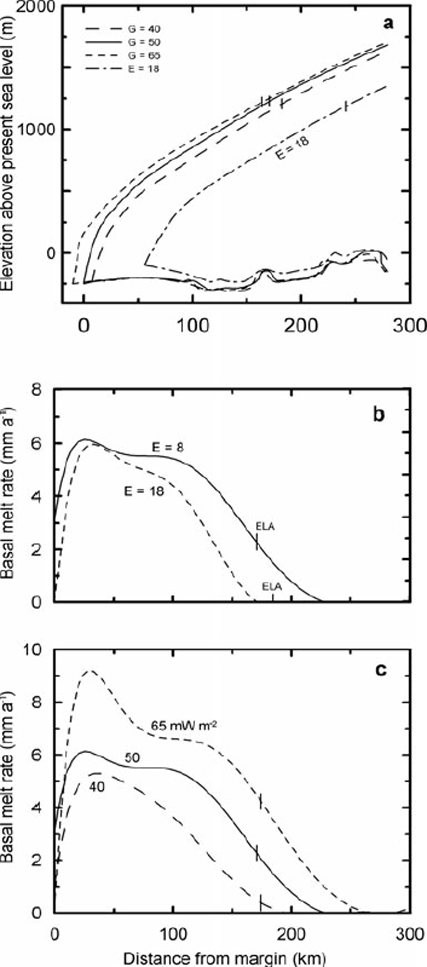
The geothermal flux averages ∼50 mW m−2 in Maine (Reference DeckerDecker, 1987), and this is the value used in our reference run. For comparison, we ran the model with geothermal fluxes of 40 and 65 mW m−2.
The enhancement factor for our reference run was 8. This is the factor needed to make the volume of ice stored in the Laurentide ice sheet equal to the volume of water lost from the oceans at the LGM and attributable to the Laurentide. We currently estimate this volume to be equivalent to 70 m of sea level. For comparison, we ran the model with an arbitrarily selected enhancement factor of 18.
We did not make runs with different values of cs because the effect can be estimated reasonably from the other runs.
With increasing geothermal flux, basal melt rates increased (Fig. 8c), resulting in a slight decrease in surface slope and a southward displacement of the 15.6 ka margin (Fig. 8a). Increasing the enhancement factor also resulted in a lower surface profile, compared with the reference run, and in a northward displacement of the margin, apparently due to a reduction in accumulation. The changes imposed resulted in changes in the basal melt rate, averaged over the outermost 200 km of the flowline, of ∼−17% (enhancement factor), ∼−29% (40 mW m−2) and ∼+40% (65 mW m−2) (Fig. 8b and c). These changes had no appreciable effect on the basal temperature gradient. Our basic conclusions would remain unaltered under any of these scenarios.
Temperature gradient in basal ice as a function of distance from the margin.
Discussion
Two key problems of esker formation can be addressed with the use of our modeling: (1) can eskers be formed in large part, or entirely, by subglacial meltwater? and (2) under what basal thermal conditions do eskers begin to form? First, however, some background will be useful.
Esker physics
A classic paper by Reference ShreveShreve (1972) provides a basis for understanding the paths eskers take. Shreve showed that, deep in a glacier, water should move in a direction normal to planes of equal hydraulic potential in the ice. These planes dip up-glacier at an angle that is ∼11 times the slope of the glacier surface. At the bed, water flows normal to contours formed by the intersections of the englacial equipotential planes with the subglacial topography. Reference ShreveShreve (1985a, Reference Shreveb) shows that this model explains some otherwise puzzling aspects of observed esker paths such as the tendency for eskers to cross divides at their lowest points, and Reference HookeHooke (2005, p.232–236) provides some simple examples applying the model.
In an englacial or subglacial conduit, dissipation of energy created by friction in the flowing water melts conduit walls. This is offset by closure of the conduit, driven by a slight difference between the pressure in the water and that in the ice (Röthlisberger, 1972;Reference ShreveShreve, 1972). The latter is approximately equal to the ice overburden pressure. In a steady state, the closure rate and melt rate are equal. Melting of the debris-laden basal ice releases the sediment that forms the esker.
Does surface water reach the bed of a polar ice sheet?
The question of whether or not surface water reaches the bed of a cold ice sheet has been previously problematic. In sufficiently cold ice, the vein system along three-grain intersections (e.g. Reference Raymond and HarrisonRaymond and Harrison, 1975) does not become enlarged enough to admit significant amounts of water to the interior of an ice sheet. Many years ago, however, Reference GlenGlen (1954) and Reference WeertmanWeertman (1973) predicted that water-filled crevasses would propagate to the glacier bed. Reference Van der VeenVan der Veen (1998) has studied this more recently. Recent field observations support the theoretical prediction. Reference Zwally, Abdalati, Herring, Larson and SabaZwally and others (2002) measured distinct seasonal changes in speed of the Greenland ice sheet at a point near the equilibrium line where the ice is ∼1200 m thick, the surface temperature is ∼–11 °C (Reference Mock and WeeksMock and Weeks, 1966;Reference Wang, Zwally and AbdalatiWang and others, 2002) and the basal temperature is at the pressuremelting point. The accelerations were in phase with melt rates at the surface. Water reached the bed through scattered moulins. Subsequently, Reference Boon and SharpBoon and Sharp (2003) documented propagation of a water-filled crevasse to the bed of John Evans Glacier on Ellesmere Island, Canada, at a point where the 15 m ice temperature was also –11°C and the ice was 150 m thick.
Esker segments
Many eskers, including those in eastern Maine, are believed to have formed in segments (e.g. Reference DonnerDonner 1965;Reference Banerjee and McDonaldBanerjee and McDonald, l975;Reference HebrandHebrand and Åmark, l989;Reference Ashley and BoothroydAshley and others, 1991;Reference BolducBolduc, 1992, p. 115). It is commonly inferred that the segments are built near the distal ends of subglacial drainage systems, and that successive segments form as the ice margin retreats. Left unexplained, however, is why tunnel deposits are not formed in the basal drainage system further up-glacier, or why segments link up as neatly as they do. Reference Banerjee and McDonaldBanerjee and McDonald (1975, p. 152), for example, concluded that ‘subglacial tunnels extend themselves headward as the ice front retreats’ but note that ‘the details of this extension are unknown’.
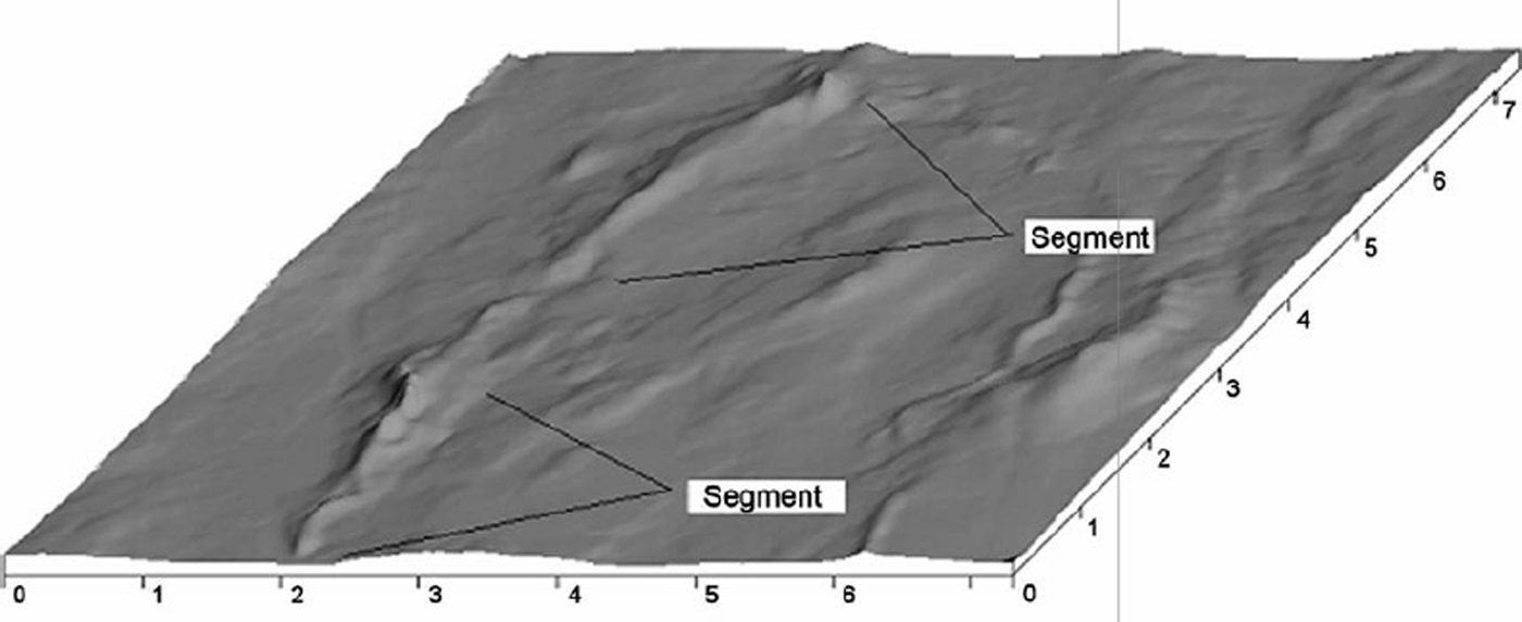
On the Katahdin esker in Maine, a typical segment begins as a relatively small ridge. The ridge increases in size downflow, at first slowly and then more rapidly, resulting in a tadpole shape (Fig. 9). We think the (tadpole) head reflects a period of time during which the margin position was relatively stable, and attribute the non-linear increase in size to: (i) melt rates on conduit walls which increase, thus releasing more sediment, as the glacier surface slope increases near the margin, and (ii) melt rates which exceed closure rates by an increasing amount as the ice thins towards the margin, resulting in a decrease in water velocity and hence in deposition in the tunnel portal. As this part of the Laurentide margin terminated in the sea, finer material that was flushed past the portal was deposited in submarine fans or, where the margin was stable long enough, in deltas. As the margin retreated, successive segments were formed. The head of each younger segment, together with its associated fan or delta, commonly laps onto and buries the tail of the previous one, like shingles. In the Katahdin esker the senior author has identified ∼30 segments, averaging ∼5 km in length.
In a meticulous study of the lithologic composition of gravels in several eskers in Labrador, Canada, Reference BolducBolduc (1992, p. 114–115) found that in some instances vertical variations in pebble lithology were reflected in longitudinal variations along the esker crest. Thus, the lithologic composition of basal beds (and the adjacent till) in one place was similar to that of beds at the esker crest 5–10 km down-flow. She interpreted this as indicating that the same time-stratigraphic unit was being sampled in both places. She then used the shingle analogy to describe how this unit was deposited on the developing esker that increased in height down-flow. Implicit in this interpretation is the assumption that the sediment load at the proximal location at any given time maintains its identity over the next 5–10 km despite dilution by new material from the tunnel walls and roof. This seems reasonable, in as much as the new material would have been coming from higher in the glacier where sediment concentrations would be lower. Headward growth of the esker along some form of pre-existing subglacial drainage system is implicit in this analogy.
Sensitivity tests: (a) effect of geothermal flux and enhancement factor on surface profile at 15.6 ka; (b) effect of enhancement factor on basal melt rate at 15.6 ka; and (c) effect of geothermal flux on basal melt rate at 15.6ka. Tick marks show locations of equilibrium lines.
In Bolduc’s case, the glacier margin was subaerial and deposition there was in the form of ‘flanking aprons’ of upward-fining sands and gravels that were, overall, finer than material in the esker. The absence of the ‘head’ may be due to a less abrupt deceleration of the flow when it emerges subaerially rather than subaqueously.
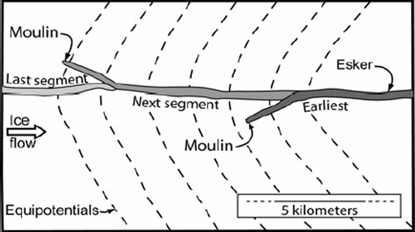
Reference ShiltsShilts (1984, p.218) thinks that eskers in the Keewatin district, west of Hudson Bay, also grew headward. He suggested that the eskers are a reflection of ‘an integrated system of drainage channels developed on the surface of the glacier’ and that ‘meltwater plunge[d] to the base of the glacier to flow in a subglacial tunnel the last few kilometers of its course’ (emphasis added). Surface drainage, however, would not necessarily follow the course defined by the potential field at the glacier bed, so new moulins would not necessarily form in precisely the right place to result in a continuous esker. Rather, where successive moulins formed in the same subglacial watershed one would expect to see barbs representing situations in which the water reached the bed on the side of a potential valley (Fig. 10). The next segment to develop would then join the earlier one some distance down-flow from the base of the moulin that initiated the earlier segment.
Oblique view, looking down-glacier, of two segments on the Katahdin esker southeast of Olamon, Maine. Based on a 30 m digital elevation model; scale in kilometers.
In short, although it is generally agreed that many eskers were built headward in onlapping segments, we have previously not had a satisfactory explanation for how they maintained their continuity as they were extended headward.
Can eskers be built by subglacial meltwater alone?
To address the question of whether eskers can be built by subglacial meltwater alone, we integrated the basal melt rate over the distance from what would probably have been the subglacial drainage divide in northern Maine to the 15.6 ka margin, a distance of ∼350 km, and multiplied it by the width of a typical flow band subtended by an esker, ∼40 km (Fig. 2). The subglacial drainage divide is judged to have been at the point where the adverse bed slope begins to consistently exceed 1.7 times the surface slope (e.g. Reference HookeHooke, 2005, p.249). It is ∼80 km north of the present topographic divide (Fig. 4). This integration yielded a discharge at the margin of 1.2m3s−1. For comparison, the runs with geothermal fluxes of 40 and 65 mW m−2 yielded discharges of 0.8 and 1.7 m3s−1, respectively. Doubling c s would have increased the discharge only to ∼1.7 m3 s−1.
To estimate the size of material that could be moved by such discharges and the size of a conduit that could carry the flow, we used Reference ParkerParker’s (1979) analysis of conditions under which sediment in gravel-bedded rivers is in general motion, adapting it to flow in a semicircular conduit of radius a. The resulting equations are:

And

where d
50 is the geometric mean particle size in meters, Q is the discharge in m3s−1, and S is the hydraulic gradient. In these equations, we tacitly assume that the conduit roughness is uniform and comparable to that in gravel-bedded rivers, thus neglecting any difference between the gravel bed and the potentially scalloped ice roof. We also assume that the roughness increases with  and decreases weakly with Q as in gravel bed rivers. With a horizontal bed, S is well approximated by the surface slope of the ice sheet. Taking S as 0.030, a reasonable mean value within a few kilometers of the margin, it appears that a discharge of 1.2 m3 s−1 could move material with d
50 = 100 mm and would produce a semicircular conduit with a radius of ∼0.64 m. Keeping in mind that 50% by weight of the material is smaller than d
50 and that some of the largest material in the eskers may have simply dropped out of the tunnel roof and not been transported any significant distance, an esker with a d
50 of 100 mm would be a moderately coarse one. Measurements at three locations on the Katahdin esker yielded estimates of d50 of 22, 32 and 46mm. These measurements were made by passing over 100 kg of material through a set of screens, weighing the material retained on the screens and measuring the long, intermediate and short axes of all material retained on the coarsest (62 mm) screen.
A flow of 1.2 m3 s−1 beneath an ice sheet with a surface slope of 0.030 would melt ∼11 m of ice per year from the walls of the conduit. If the debris content of the ice were 6% by volume, it would take ∼210 years to accumulate an esker segment 10m high with 15° side slopes and 25% porosity. This is roughly the average size of the Katahdin esker. The ice front retreated about 120 km between 16 and 14 ka. If it took 210 years to build a segment, only ∼10 segments could have been built rather than the ∼25 observed over this distance, and segments would average ∼13 km in length rather than ∼5 km as observed. Furthermore, a 6% sediment concentration is probably the upper limit of likelihood, particularly 10 m above the bed, near the top of a typical esker segment. Thus, it seems that subglacial meltwater alone, although capable of moving the material in the Katahdin esker, is probably not sufficient to build it. Adding superglacial water to bring the total to 6.5 m3 s−1 brings the calculations within reasonable limits. Then, with a 3% sediment concentration a 5 km segment could accumulate in ∼ 80 years, and 25 segments could be built in 2 ka.
Plan geometry of a hypothetical segmented esker built by water that reached the bed through moulins. It is assumed that successive moulins are formed as the ice sheet retreats, that the esker begins at the bottom of the moulin and that it subsequently connects with the previously formed segment. Moulins are unlikely to form exactly on the axis of the potential valley. Barbs are therefore expected.
However, if surface water was involved, we are faced with the crucial problem mentioned above: why do esker segments line up to form a continuous ridge?
Why do segments line up?
The basal temperature gradient conducts heat upwards into the ice. This reduces the heat available for releasing debris by melting of conduit walls, and thus may play a significant role in determining where eskers begin to form. Consider a situation in which the subglacial water flux is distributed in an anastomosing network of broad low channels occupying a certain fraction f of the glacier bed in a flow band of width w. Noting that the hydraulic radius is one-half the channel depth d, we find from the Gaukler–Manning–Strickler equation that:

where n is the Manning friction coefficient. Based on dye trace experiments on Storglaciären, Sweden, we take n = 0.1 m−1/3 s for a shallow subglacial conduit on a rough bed (Reference Seaberg, Seaberg and HookeSeaberg and others, 1988, p.225). Then, choosing f = 0.2, w = 40 km, integrating the melt rate outward from the divide to obtain Q, and using the surface profile for 15.6ka in Figure 4 to obtain S, we find that d increases outward from 0 at the subglacial drainage divide to a maximum of ∼6 mm, 45 km from the margin. The flow velocity is then ∼19 mms”1. These appear to be reasonable values. Closer to the margin the depth decreases in response to the increasing potential gradient resulting from the increasing surface slope.
Now suppose that the heat dissipated by water flowing in one of the anabranches of this network begins to melt a conduit upwards into the ice, deepening the flow. The increase in discharge in the deeper anabranch will result in an increase in energy dissipation there, and under temperate ice this will result in further melting. Owing to this positive feedback, Reference ShreveShreve (1985a, p. 642) suggested that the resulting conduit would become ‘sharply arched’. The pressure in this conduit will normally be lower than that in smaller anabranches (Röthlisberger, 1972;Reference ShreveShreve, 1972), creating a tendency for flow from the latter to the former and hence in further enlargement of the developing conduit.
Calculated temperature distribution in cold ice above a conduit at the pressure-melting point. ß 0 is taken to be −0.03 Km−1.
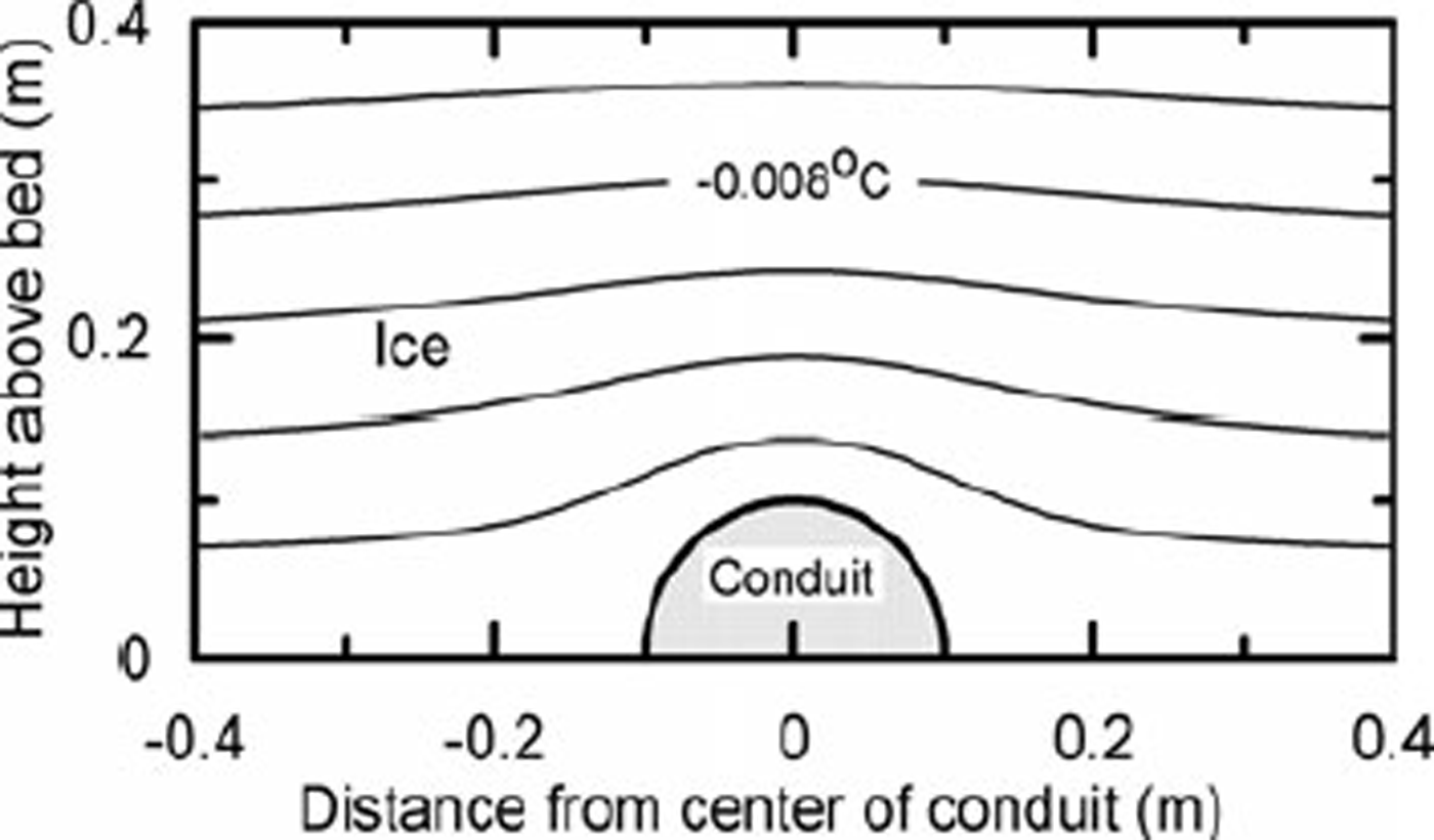
Under cold ice, in situations in which the temperature decreases with height above the bed, the conduit roof must still remain at the pressure-melting point. Thus, the temperature contours immediately above the conduit must be deflected upward relative to those a long distance from it (Fig. 11). Far above the conduit, however, the contours will not be affected. Thus the temperature gradient above the conduit will be higher than elsewhere along the bed, and heat loss from the conduit will be greater. This will inhibit melting of the conduit roof, and hence limit release of debris from the ice. Under suitable conditions, this may prevent formation of an esker.
To partially quantify this argument, consider the temperature distribution around a semicircular conduit (Fig. 11). We ignore advective effects such as flow of ice towards the conduit, and consider only heat conduction. The problem resembles that of flow of an ideal incompressible fluid past a cylinder inasmuch as both involve solutions to the Laplace equation. Adapting a solution to the latter problem (Reference Ablowitz and FokasAblowitz and Fokas, 1997, p. 40–43) yields:

where T is the temperature and r is the radial distance in the direction θ from the center of the conduit. Heat loss through the conduit wall is proportional to the temperature gradient βa in the ice at r = a. From Equation (3),

Thus, the steady-state heat loss varies sinusoidally from 0 at θ = 0 (parallel to the bed) to twice the average at θ = π/2. Over the top of a developing conduit, the heat loss will actually be greater than this because the temperature distribution will not have had time to adjust to the presence of the conduit and because any advection of ice toward the conduit will increase ßa . Thus, while a rigorous analysis would have to treat this as a moving boundary problem and include advective effects, the present steady-state analysis is conservative.
The total heat loss from the conduit in the steady state EL is:

where Ki is the thermal conductivity of ice. This is twice the heat loss through a planar ice/bed interface of width 2a, corresponding to the situation in the absence of the conduit. The minus sign reflects the fact that ßo is negative (because the z axis is positive upwards), so the loss is positive.
Let us now return to the conduit developing in a broad low anabranch of the distributed drainage network. Energy is produced in this conduit by viscous dissipation in the flowing water, Ep , is augmented by geothermal heat, Eg , and is consumed by melting, Em . Here we neglect: (i) energy dissipated in the water as the water layer is sheared over the bed by the overlying ice, and (ii) energy dissipated by straining in basal ice on either side of the conduit. In a wide, shallow anabranch, the steady-state energy balance is: Ep + Eg − Em = El. EL is proportional to ßo , and ßo is fixed by external factors. Em is the independent variable, fixed by the values of the three other terms. If the depth of flow in the anabranch is increased slightly by melting of the roof, E g remains unchanged, E p increases and as ßo →ßa, E L also increases. If ß o ≥ 0 (ice isothermal or becoming warmer with increasing height above the conduit) or ΔEp > ΔE L, however, Em will increase and the conduit may then develop a sharply arched form. The question is therefore: when ß 0 < 0 how large does an evolving sharply arched conduit (approximated by a semicircular form) have to become before ΔEp exceeds ΔE L? Because the energy loss from a semicircular conduit of radius a is twice that from a broad flat conduit of depth d and width 2a, we want to know the radius at which Ep is double that of the flat conduit.
At a fixed point on the bed, E p is proportional to Q (e.g. Reference HookeHooke, 2005, p.205–206). Using the Gaukler–Manning– Strickler equation to express Q in terms of the depth d and width 2a of the initial sheet flow and radius a of the developing semicircular conduit, we find that the critical radius is:

Thus, as long as ßo < 0 in the basal ice, a sheet flow would have to evolve into a semicircular conduit with nearly triple the depth before heat produced in the deeper flow would balance the additional loss.
Uncertainties in this calculation include the effect of bed irregularities, the change in ßo when a flat roof of a broad conduit is perturbed into a more realistic sinusoidal shape, the amount by which ßo would be amplified if the problem were solved as a moving boundary problem and the role of the magnitude of ßo . Nonetheless, we suggest that beneath cold ice this process dampens the tendency for a broad flat conduit to evolve into a sharply arched conduit by melting of the roof. Without such melting, sediment will not be released from the ice and eskers will not form.
Towards the margin, as ßo →0, the tendency for perturbations to be dampened probably decreases. Among other things, the initial transient amplification of ßa as temperature contours adjust above the conduit will be weaker. We therefore suspect that arched conduits develop before ßo = 0.
Geomorphic implications
The foregoing analysis applies to an ice sheet resting on a plane bed; esker systems in Maine, however, are located within topography that ranges from undulating hills to low mountains. Furthermore, we have not yet added water from the glacier surface.
We offer the following plausible qualitative scenario. Basal meltwater flows in a distributed system of broad low conduits throughout most of its journey to the margin. Within a few kilometers or few tens of kilometers of the margin, however, moulins develop by propagation of waterfilled crevasses to the bed. Water descending into the moulins encounters a distributed drainage system on a valley side in the potential field at the bed (Fig. 10) and flows down the valley side in this distributed system. In the valley bottom, it joins flow from further up-glacier. As the flow approaches the margin, the magnitude of the temperature gradient in the basal ice decreases until a sharply arched conduit can form. Within the conduit, an esker forms.
Our modeling and calculations suggest that eskers may form only near the margin as further up-glacier temperature gradients in the basal ice prevent the development of arched conduits with melting walls (that supply sediment). Water may therefore reach the bed through moulins further from the margin, but it then spreads out in a distributed drainage system. The correlation between surface melt rates and ice velocity in Greenland (Reference Zwally, Abdalati, Herring, Larson and SabaZwally and others, 2002), for example, suggests the presence of a distributed subglacial drainage system. As arched conduits with lower water pressure begin to develop nearer the margin, water is drawn out of the distributed system into an arborescent system.
This analysis also provides a possible explanation for another interesting characteristic of glacial landforms in eastern Maine. Prior to ∼16 ka, water emerging from beneath the ice sheet built submarine ridges of stratified sand and gravel parallel to the margin (Reference KaplanKaplan, 1999). The continuity of these grounding line moraines, their internal structure suggestive of coalescing fans, and their undulating profiles parallel to the margin suggest that the water emerged in many small conduits spaced only hundreds of meters apart (personal communication from H.W. Reference Boon and SharpBorns, Jr, 2007). This mode of sedimentation continued during the pause in retreat just inland from the present coast at ∼15.6 ka. The huge Pineo Ridge moraine was built at this time. Thereafter, however, moraines ceased to develop; instead, sedimentation took the form of massive eskers. This transition may mark the transition from a distributed drainage maintained by high negative temperature gradients in the basal ice to a more channelized drainage permitted by a wider marginal zone with less negative basal temperature gradients.
To summarize, our calculations (1) suggest that the Katahdin esker was probably not formed entirely by water generated by subglacial melting, and (2) provide a possible explanation for the observation that many eskers are built in segments. The calculations, however, are subject to considerable uncertainty; they support the plausibility of our conceptual model of esker development, but do not prove its validity.
Conclusions
Our numerical modeling of the retreat of the Laurentide ice sheet in Maine suggests that the ice surface slope may have increased during retreat, that melting conditions obtained over most but not all of the glacier bed in Maine and that the temperature gradient in the basal ice was elevated within 200 km of the margin. Calculations suggest that basal melt rates were not sufficient to produce eskers without additional input of water from the ice surface, and that temperature gradients in the basal ice may have inhibited conduit formation at distances greater than a few kilometers from the glacier margin.
Acknowledgements
R.L.H. is indebted to F. NG for pointing out an error in an early version of Equation (4) and for clarifying other aspects of that solution. Conversations with many people over the years have fueled R.L.H.’s interest in eskers and sharpened his ideas. Deserving special mention is R. Shreve who carefully and exhaustively reviewed three earlier versions of this paper, resulting in many significant improvements (although we apparently have not convinced him that the Laurentide ice sheet in Maine was polar, that the Katahdin esker was built headward in segments, and that the University of Maine Ice Sheet model is up to the task we have given it). We also extend our thanks to J. Kleman and G. Ashley who also constructively criticized earlier drafts, and to W. Warren.
Appendix A
Interpolation along the boundary of the higher-resolution area uses bilinear spatial and linear temporal interpolation. A higher-resolution embedded node locates the nearest lower-resolution embedding node in each of four quadrants and treats these as corners of a quadrilateral in which standard finite-element method (FEM) machinery, using a bilinear function of the form V(x, y) = A + Bx + Cy + Dxy, can be used (Reference Becker and CareyBecker and others, 1981). Having found spatially interpolated values for a node at two different times, simple linear interpolation is used to find the value at the required time. The nested grids used in this exercise start with 100km grid spacing and 25 year time-steps (smaller than necessary) for the whole Laurentide ice sheet, and progress to a regional grid with 35km spacing and 25 year steps. The final highest-resolution grid for the state of Maine uses a 12 km grid with 5 year time-steps. Since interpolation is only along the margins of the embedded grid, behavior in the interior represents a higher-accuracy representation of the solution. This is not unlike the usual situation in FEM where a variable grid spacing is used to represent a solution with more or less detail in different areas of the domain (see Reference Becker and CareyBecker and others, 1981, for details of the convergence of the FEM solution as element size is reduced).
Appendix B
The temperature calculation is a one-dimensional timedependent calculation at each node, with Dirichlet boundary conditions at the top surface and Neumann boundary conditions at the bed (subject to the condition that the bed temperature cannot exceed the pressure-melting point). To include the effects of longitudinal heat advection, we used a modification of an approach suggested by Budd (see Reference BuddBudd, 1969, p. 87, or Reference HookeHooke, 2005, p. 131–135) in which the longitudinal rate of warming in the ice is approximated by usiαλ. Here, u si is the part of the horizontal velocity at the surface that is due to internal deformation, α is the surface slope and λ is the lapse rate. (If the horizontal velocity due to sliding is included, impossibly cold internal temperatures are obtained because temperature gradients near the surface increase and supply the heat necessary to obtain the usiαλ warming rate (Reference Hooke and GouldHooke, 1977, p.9;2005, p. 138).) Since sliding velocities are high, our procedure is a relatively crude approximation of reality, but it does have the realistic effect of reducing basal temperatures and melt rates. This warming rate is added to the source term, i.e. the term including internal shear heating (also calculated as a function of depth). Advection acts not like a heat source, but like a sink as it cools.



