


1. Introduction
Quantum chemistry is the use of quantum mechanics (and quantum field theory) to model molecules and their dynamics, with the aim of explaining and predicting their chemical properties and reactions.Footnote 1 Its status is important to questions about the place of physics among the sciences: prima facie, quantum chemistry is an example of the success of reductionism, exemplifying the fundamentality of physics with respect to chemistry and other natural sciences.Footnote 2 However, the received view in the philosophy of quantum chemistry is that attention to models and scientific practice reveals not only that quantum chemistry does not reduce to quantum physics, but that the two are explicitly in conflict. One principal argument for this view is based upon alleged non-quantum features of the ‘Born–Oppenheimer approximation’ (BO), which is the most commonly used model of molecular dynamics in quantum chemistry. It has been claimed in the philosophy literature that BO violates the Heisenberg uncertainty principle, and so is in conflict with quantum theory.Footnote 3
For instance, in an influential essay supporting anti-reductionism concerning the chemistry–physics relation (citing a talk by Olimpia Lombardi), Hasok Chang asserts that
… the typical method of quantum-mechanical treatment of molecules begins with the Born–Oppenheimer approximation, which separates out the nuclear wavefunction from the electronic wavefunction […] Additionally, it is assumed that the nuclei have fixed positions in space. In this ‘clamping-down’ approximation, the atomic nuclei are treated essentially as classical particles; as Olimpia Lombardi points out, this picture is non-quantum in a very fundamental way as the simultaneous assignment of fixed positions and fixed momenta (namely, zero) to them violates the Heisenberg uncertainty principle. But without such classical scene-setting, the quantum calculations are quite impossible. (Chang Reference Chang, Simões, Renn and Arabatzis2015, p. 198)
In our terms, Chang claims that BO involves both the separation of wavefunctions (which is what he calls ‘the Born–Oppenheimer approximation’) and a ‘clamping-down’ approximation, and that the latter violates the Heisenberg uncertainty principle, so BO as a whole is not fully quantum. Note that the claim is of ‘violation’ of the principle rather than a mere conceptual or practical conflict. Lombardi (Reference Lombardi2023) puts it even more strongly. When endorsing Torretti’s (Reference Torretti, Agazzi and Pauri2000) view that bringing together theories without worrying about their incompatibility, seemingly ‘outrageously’ (p. 119), is nonetheless scientifically legitimate on pragmatic grounds, she notes that BO
as used in the context of quantum chemistry, is a vivid example of how scientists ‘outrageously’ appeal to incompatible theories in their practice. In this case, quantum chemical models of molecules are obtained by combining classical mechanics to describe the nuclei and quantum mechanics to account for the motion of the electrons. (p. 115)
Lombardi and Chang’s idea that BO violates Heisenberg uncertainty grounds more general anti-reductionist claims (Accorinti and González Reference Accorinti, González, Lombardi, González and Fortin2022; Cartwright Reference Cartwright2022). Cartwright argues that the alleged violation implies not only that chemistry fails to reduce to physics, but that the two are inconsistent.Footnote 4 After quoting the passage from Chang above (without reference to Lombardi et al.), Cartwright says:
This approximation treats the atomic nucleus as a classical particle. But this fundamentally violates quantum mechanics which, following the Heisenberg uncertainty principle, maintains that we cannot have a simultaneous assignment of fixed positions and fixed momenta. The approximations that provide the reduction violate the very theory that the chemistry is being reduced to […] the success of quantum chemistry relies fundamentally on assumptions that belong to classical chemistry (Cartwright Reference Cartwright2022, pp. 106–7)
Note the claim is that the approximation ‘fundamentally violates quantum mechanics’.
To our knowledge, the idea that BO might violate the Heisenberg uncertainty principle has never been discussed in the considerable mathematical physics literature that has been devoted to the study and development of BO. Indeed, from a mathematical perspective, a genuine violation of the Heisenberg uncertainty principle could only occur in a context beyond the Hilbert space representation of states and observables that is core to BO.Footnote 5 Thus, according to the basic structure of the model, there is simply no possibility for the uncertainty principle to be violated. This notwithstanding, versions of the erroneous claim that it does have been expressed (largely informally) with the quantum chemistry literature.Footnote 6
The first aim of this paper is to demonstrate unambiguously that BO does not violate the Heisenberg uncertainty principle. Footnote 7 We show this by analysing a textbook-style presentation of the modern BO, given in sections 3.2 and 3.3, which we contrast with historical versions (section 3.1). Of course, there is more to chemistry than can be shown using BO, so our demonstration does not suffice to show its reduction to physics. However, it does clarify the relation, and refute one powerful anti-reductionist argument.
The second aim of this paper is to provide an account of the idealizations operative within the modern version of BO. We first analyse the structure of BO as an idealized quantum mechanical model. We then provide justification for the key idealization within the model based upon the stability of the salient model-based inferences regarding the behaviour of molecules under de-idealization. We present the core details of this analysis in section 2 and a more detailed justification in section 3.2.
The third aim of this paper is to address concerns about the rigour of the textbook presentation of BO; in particular, subtle issues regarding the justification of the mathematical idealizations involved in modern formalizations and the assumptions needed in the derivation of a discrete spectrum. First, Sutcliffe and Woolley (Reference Sutcliffe and Guy Woolley2012, Reference Sutcliffe, Guy Woolley, Hotokka, Brändas, Maruani and Delgado-Barrio2013) articulate convincing criticism of Born and Huang (Reference Born and Huang1954), regarding the spectrum of the ‘electronic Hamiltonian’ and the interpretation of BO as a perturbative analysis. In section 4 we summarize this issue and argue that it does not apply to our presentation of BO. We also highlight the analysis of Jecko (Reference Jecko2014), whose stated goal was to temper Sutcliffe and Woolley’s ‘pessimism’ about the tenability of BO as a quantum approximation, by outlining how mathematical physics has provided a rigorous approach to BO.
The fourth and final aim of this paper is to use the analysis of BO to open up wider questions concerning the role of reduction and rigour in quantum chemistry. Section 5 provides a prospectus for future philosophical work on the foundations of quantum chemistry that is informed by scientific practice, as all parties agree that it should be. We argue that such philosophical work should be disentangled from the unwarranted mobilization of quantum chemistry against the fundamentality of physics. We show that attending instead to the conceptual, formal, and methodological questions which scientists themselves ask raises a range of issues and open questions relating to the various types of semi-classical modelling, the role of persistent environmental interactions, and the problem of isolating distinctively ‘chemical’ modes of quantum modelling practice.
2. Idealized quantum models of molecules
When quantum chemists and physicists talk about BO they refer to an approach to solving the quantum mechanical equations for a molecule, based on an idealized quantum model of a molecule that builds on – but modifies and extends – pioneering work by Born and Oppenheimer in 1927. Before going into detail, it will be helpful to give an overview of BO, its idealizations, and their rationale.
The basic idea is to use to the high ratio between the electron and nuclear masses to produce trial solutions to a molecular Schrödinger equation; we consider the time-independent equation, but the method extends to dynamical problems as well. There are two distinct aspects of BO: a separation ansatz and an adiabatic approximation. The ansatz is that the molecular wavefunction,
 $\Psi(x_1,x_2)$
, is approximated by the product of a function of nuclei positions,
 $\theta_a(x_1)$
, and a (specified) function of nuclei and electron positions,
 $ \psi_a(x_1,x_2)$
, so that we have
 $\Psi(x_1,x_2) = \theta_a(x_1)\psi_a(x_1,x_2)$
. The approximation is that the rate of change of the
 $\psi_a(x_1,x_2)$
with respect to the nuclear position is approximately zero; this condition provides an equation for
 $\theta_a(x_1)$
.
The arguments of Lombardi and Castagnino (Reference Lombardi and Castagnino2010), González et al. (Reference González, Fortin and Lombardi2019), and Fortin and Lombardi (Reference Fortin and Lombardi2021) (and perhaps also of Chang (Reference Chang, Simões, Renn and Arabatzis2015), which endorses Lombardi’s analysis in the passage above but does not otherwise elaborate) involve a misrepresentation of how BO is justified in quantum chemical practice. This is not done, as they suggest, by idealizing the nuclei as classical, but by a quantum theoretical idealization about energy levels, justified by its stability under de-idealization (as in many other cases). The intuitive idea is that the total kinetic energy of the nuclei is small compared to the sum of the potential energy of the molecule and the total kinetic energy of the electrons. This is because a nucleon is far heavier than an electron, and so typically moves far more slowly, and kinetic energy scales as
 $mv^2$
.
Mathematically,
 $\psi_a(x_1,x_2)$
is a family of electron (
 $x_2$
) wavefunctions, one for each fixed nuclei configuration (
 $x_1$
). Each function in the family is an eigenstate of a so-called ‘clamped Hamiltonian’, the sum of terms for the kinetic energy and potential energy of the electrons, given that nuclei configuration.Footnote
8
The corresponding family of energy eigenvalues
 $\lambda_a(x_1)$
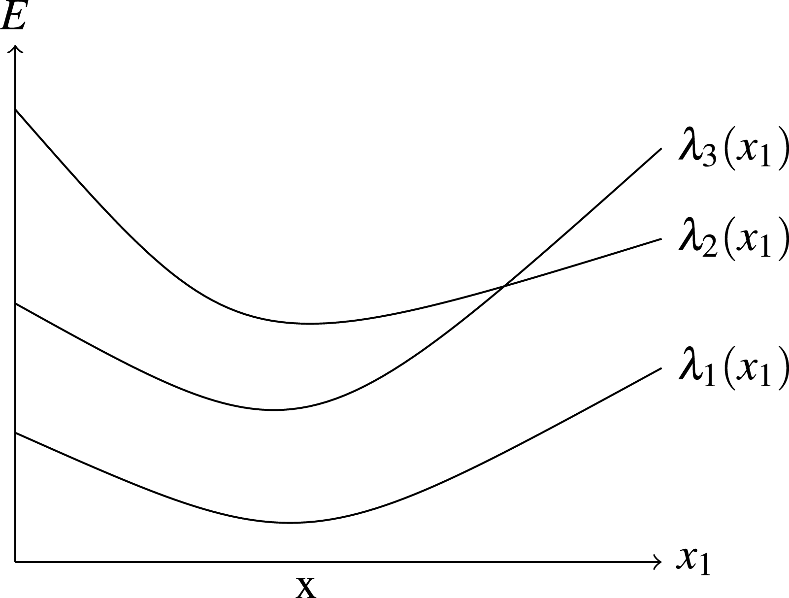
picks out a ‘potential energy surface’ (PES) as illustrated in figure 1. (Section 3.2 explains in detail why it would be a confusion to think that these merely formal facts in any way amount to idealizing the nuclei as classical.)
 $\theta_a(x_1)$
is, formally speaking again, a wavefunction for the nuclei in this potential. The molecular energy is approximately the sum of
 $\lambda_a(x_1)$
and the nuclear kinetic energy, and because of the energy difference, close to the former (for any relevant
 $x_1$
). So if the gaps between the
 $\lambda_a(x_1)$
are large, only one
 $\psi_a(x_1,x_2)$
is relevant to
 $\Psi(x_1,x_2)$
– superposing with other eigenstates of the clamped Hamiltonian shifts the energy too far. Figure 1 shows the crucial representative features of the PESs. It makes clear that energy gaps do not exist for all values of
 $x_1$
. It also illustrates that the gap can exist for a given range of values, about a minimum.
Eigenvalues
 $\lambda_n$
of the clamped Hamiltonian, as (hypothetical) functions of the heavy, nuclear degrees of freedom
 $x_1$
. In the region around
 $x_1=\rm{x}$
the first three electronic energy levels can be seen to be widely separated; specifically, by far more than the kinetic energy of the nuclei. This is the condition for stable molecules, and for BO.

One expects that the nuclei of a stable molecule are restricted to a region around such a point; the nuclear wavefunction effectively vanishes outside. Thus the more specific assumption made in BO is:
Heavy: In a stable molecule the nuclei are approximately localized, in a quantum state in which their kinetic energy is much smaller than the electron kinetic energy (though not zero).
In section 3.2, once some of the necessary formalism has been developed, we show how (a precisification of) this assumption justifies the separation ansatz and adiabatic approximation, and hence BO, in quantum mechanical terms. We emphasize that this justification does not involve taking nuclear masses to infinity; indeed, such a limit is not generally well defined (Frolov Reference Frolov1999; Sutcliffe and Woolley Reference Sutcliffe and Guy Woolley2012). Manifestly, Heavy does not assert the existence of such a limit.
The idealized model is one in which Heavy holds for any nuclear configuration,
 $x_1$
, corresponding to a stable molecule. That is, the energy gaps exist for all values of
 $x_1$
. In BO, generically, they do not: there are regions like that in figure 1 in which the levels cross, and the idealization fails. However, on one standard account of idealization, inferences based upon an idealized model are justified to the extent that they are stable under relaxation of the idealization (McMullin Reference McMullin1985; Landsman Reference Landsman2013; Earman Reference Earman2004).Footnote
9
Suppose, then, that Heavy is valid in the region in which the nuclei are effectively restricted. Then, to the extent that the support of the full molecular wavefunction lies in the region in which Heavy holds, we can expect the wavefunction to remain approximately separable – for stability under de-idealization.Footnote
10
We return to this point in section 3.2.
The idealized model includes a false assumption regarding the range of validity of Heavy, but does not involve any assertions inconsistent with quantum theory. By contrast, consider an alternative idealizing assumption of the form:
Clamped: Molecular nuclei have fixed definite positions and zero kinetic energy.Footnote 11
An idealized model of which Clamped is true would be one in which molecular nuclei have classical positions and momenta (namely zero), in conflict with the Heisenberg uncertainty principle, as claimed in the quoted passages. In such a model it would be plausible to argue that a classical modelling procedure is required to apply the approximations involved (even if it is only one half of an ‘outrageous’ classical-quantum combination ultimately delivering a fully quantum solution). However, the authors mentioned above do not show that such an idealization is part of the form of BO which we discuss below (or indeed its original form). Nor does use of the family of clamped Hamiltonians assume Clamped, which effectively selects one of them. Moreover, Heavy is a much weaker assumption than Clamped and consistent with the nucleus being fully quantum. Indeed, (a precisification of) Heavy justifies the separation ansatz and adiabatic approximation, and hence justifies BO, in quantum theoretic terms. This demonstration involves neither of the stronger (arguably false) assumptions of a mass limit or Clamped. All these things are shown in sections 3.2 and 3.3, the core of our argument concerning BO.
To summarize, our argument regarding idealizations and BO is as follows:
Idealization and BO:
-
I1 Idealized models are related to less idealized models via approximation relations.
-
I2 Inferences based upon idealized models are justified if the features of the idealized model that ground the relevant inference are stable under de-idealization.
-
I3 The fundamental idealization of BO is Heavy. Inferences about the behaviour of molecules in the relevant regime are indeed stable under de-idealization.
-
I4 BO does not involve the idealization Clamped.
-
I5 The conflict with the Heisenberg uncertainly relation (and stability under de-idealization) of Clamped is irrelevant to the use of models based on BO.
3. The Born–Oppenheimer approximation
3.1. The historical treatment
What we can call the ‘perturbative expansion Born–Oppenheimer approximation’ (PBO) is the approach to the approximate solution of the (time-independent) Schrödinger equation for stable molecules pioneered by Born and Oppenheimer in their 1927 paper Zur Quantentheorie der Molekeln (‘On the Quantum Theory of Molecules’).Footnote
12
The key physical feature upon which PBO is built is that nuclei are very much heavier than electrons. With this in mind, Born and Oppenheimer introduce a small parameter,
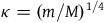 $\kappa = ({m}/{M})^{1/4}$
, where m is the electron mass and M the nucleon mass; the ratio
 $m/M$
is roughly
 $1/2000$
so
 $\kappa\approx0.15$
. The crucial idea is to treat the nuclear kinetic energy as a perturbation of the energy, expanded in powers of
 $\kappa$
. The original PBO is indicated by the authors to be valid from zeroth to fourth order in
 $\kappa$
with nuclear vibrational energy corresponding to terms of second order and the rotational energy to fourth order in the energy. Coupling effects among electronic states appear beyond fourth order in
 $\kappa$
.
The principal achievement of PBO is to show that one can use the Hamiltonian for electrons in the Coulomb field of a fixed nuclear configuration to construct a family of electronic wavefunctions. These wavefunctions can then be used to calculate approximate eigenvalues for the full molecular Hamiltonian on the assumption that the nuclear motion is confined to a small vicinity of a privileged equilibrium configuration. Up to order
 $\kappa^4$
, approximate wavefunctions can then be written as products of an ‘electronic’ wavefunction and ‘nuclear’ wavefunctions (Sutcliffe and Woolley Reference Sutcliffe and Guy Woolley2012, p. 3) – the physical significance of these objects is discussed in more detail in following sections.
The seeds of later confusion were sown in the description that Born and Oppenheimer provide of the zeroth-order equations. In particular, Part II of the paper, titled ‘Electronic Motion for Stationary Nuclei’, states that ‘if one sets
 $\kappa=0$
one obtains a differential equation in the [electron position variables] alone, the [nuclear position variables] appearing as parameters’. The solution of such an equation is then indicated to ‘represent the electronic motion for stationary nuclei’. As noted by Sutcliffe and Woolley (Reference Sutcliffe and Guy Woolley2012), ‘it is perhaps to this statement that the idea of an electronic Hamiltonian with fixed nuclei as arising by letting the nuclear masses increase without limit, can be traced’ (p. 2).
Yet, the representational content of a perturbative model should not be conflated with its zeroth-order terms, on pain of misunderstanding their ubiquitous use as scientific models. PBO does not represent the nuclei as fixed; rather, it organizes an expansion in which only the leading, zeroth-order, term has that character. It expands around a fictitious system in which the nuclei are clamped. These are entirely different modelling strategies. (Analogously, one should not conflate a purely Newtonian model with a perturbative expansion involving the Newtonian model plus relativistic corrections.) The result of PBO is, of course, (in principle) a wavefunction that satisfies the uncertainty relations for both electrons and nuclei. Thus, the idealizing assumption Clamped does not form part of PBO and the idealization problem does not occur.Footnote 13
PBO was made redundant by later work of Born (Reference Born1951) and Born and Huang (Reference Born and Huang1954), and it is that approach that is today referred to in chemistry literature as defining the ‘Born–Oppenheimer approximation’ and to which we now turn.
3.2. A textbook-style presentation: Preliminaries
This section and the next are a treatment of the current BO, drawing in parts upon Messiah (Reference Messiah1962) and Jecko (Reference Jecko2014), but with no serious attempt at historical reconstruction. Here, ‘textbook-style’ indicates both accessibility and an emphasis on heuristics over rigour at certain points. In particular, the pedagogical aim of a textbook may be to sketch the overall logic of a calculational method in order to emphasize certain principles, so that the method is memorable and portable to related problems in scientific practice. In the process certain idealizations have to be made, which should be justified by a more rigorous de-idealization in the background. Our treatment similarly describes the overall logic of BO in a way to make clear its quantum nature; it makes certain idealizations, (some of) which are flagged below and addressed in detail in section 4. In presenting at this level of informality we follow our interlocutors, while aiming to deepen the level of mathematical precision in philosophical discussions of BO.
Suppose a system is comprised of two parts, with canonical variables
 $x_1 \in \mathbb{R}^m$
and
 $x_2 \in \mathbb{R}^n$
. In the usual way, the state of the system in the x-representation – the wavefunction – is
 $\Psi(x_1,x_2)\in {L}^2({\mathbb{R}}^m \times \mathbb{R}^n)$
, and (setting
 $\hbar=1$
) the canonically conjugate observables are
 $i\partial/\partial x_j$
. The (non-relativistic) Hamiltonian is the sum of kinetic,
 $\hat T_j$
, and interaction,
 $\hat W$
, parts:
 ${\hat H} ={\hat T}_1 +{\hat T}_2 +{\hat W},$
with
 $\hat W$
some function of the variables
 $x_j$
, and
 ${\hat T}_j$
a power (or sum of powers) of the corresponding conjugate variables,
 $\partial^n/\partial x_j^n$
. In the case of a molecule, the first two terms will be the kinetic energies of nuclei and electrons (
 $\hat p_j^2/2m \propto -\partial^2/\partial x^2_j$
), respectively, and the third, Coulombic potential energy.Footnote
14
We are interested in finding the eigenstates of
 $\hat H$
, which cannot be done analytically, but requires approximation (at least in practice). So suppose further – and this is the crucial assumption – that in a range of states of interest the kinetic energy of the
 $x_1$
subsystem is far smaller than both that of the
 $x_2$
part and that of their interaction energy:
 $T_1 \ll T_2, W$
(where O denotes the expected value of observable
 $\hat O$
). What ‘range of states’? In the first place, those wavefunctions that only have (non-negligible) support in a finite range of values of
 $x_1$
; the first system is effectively localized within that region. (Moreover, the states should be below some maximum energy level.)
The crucial assumption (elaborated and sharpened below) is a mathematical ansatz, a temporary supposition made to find solutions to an equation, which must then be inspected to verify that they really solve it. If so, the supposition is vindicated; if not, then it must be given up. For example, a familiar move when solving a differential equation for a function in two variables is to see whether it is the product of functions of only one variable,
 $F(x,y)=f(x)\cdot g(y)$
. There are tests for such separability (which is not the same as that in BO), but they do not apply generally, and even when they do it may be simpler to try to solve the equation under the ansatz. If one is lucky then one finds such a function that demonstrably solves the equation, and one knows, rather than supposes, that there is a separable solution; if one is unlucky then of course the ansatz is rejected. An ansatz is then not intrinsically an approximation or idealization, but a guess, whose proof is in the eating. However, one might make the ansatz that an approximate solution of a certain kind exists: that a separable function approximates a true solution, say. Naturally, any such function would then have to be checked to see if it was an approximate solution, to see whether the guess was good. We stress that whether the ansatz postulates a feature of exact or approximate solutions, it never changes those solutions; it just guesses what they are in fact like. All of this is a completely standard heuristic in mathematics, in science, and indeed in any reasoning, though it seems to have had little explicit discussion in philosophy.
One can seek motivation for making an ansatz, a reason to think that it will turn out to be true of some solution. But such motivation should not be understood as its justification – if an ansatz is justified, it is wholly by the solutions it produces. In the present case the ansatz made to solve the molecular Schrödinger equation – the crucial assumption – is motivated by the composition of a molecule, in which the nuclei comprise the first system, and the electrons the second. In typical states, because electrons are 2000 times lighter than nucleons, they are more easily set in motion, and a stable state is one in which almost all the kinetic energy is in the motion of the former; if it is a low-energy state then the nuclei can only be displaced from a potential energy minimum by a small amount (Messiah Reference Messiah1962, XVIII.12). Notice that this motivation mixes physical and mathematical considerations: appealing to the physical features represented by elements of the formalism, and expectations about their physical behaviour. The justification, however, is purely mathematical: finding (approximate) solutions to the Schrödinger equation in which the guess is true. Moreover, as indicated in section 2, such confirmation also demonstrates stability under relaxation of the idealizations involved, again by showing that the (in practice approximate) solutions of idealized model remain approximate solutions of the (more) exact equations.
To see the role of the crucial assumption in finding (approximate) eigenstates of
 $\hat H$
, we first consider normalized solutions to the (time-independent) Schrödinger equation for the ‘clamped’ Hamiltonian (in the x-representation) for a specified value of
 $x_1$
:
 $({\hat T}_2 + {\hat W}(x_1)){\psi}_a(x_1;x_2) = {\lambda}_a(x_1){\psi}_a(x_1;x_2),$
with
 $a=1,2,$
…Footnote
15
We cannot stress strongly enough that here we are thinking purely mathematically, about some formal properties of this equation, and are not taking the equation to represent – even approximately – anything physical, including a molecule. It it were to represent something, it could be a fictional collection of electrons moving in the field of some fixed, or ‘clamped’, charges. (The constants that appear in (2) are numerically equal to the masses and charges of molecular constituents.) But at present we are speaking formally, about the mathematics, not materially about any molecules. Indeed, as we are showing, at no point in BO does a single clamped Hamiltonian represent the molecule under consideration.
Since different values for
 $x_1\in\mathbb{R}^m$
could be specified, there is a parameterized family of
 $x_2$
operators
 ${\hat W}(x_1)$
, so there is not just one but infinitely many clamped Hamiltonians. In that case, the
 ${\hat T}_2 + {\hat W}(x_1)$
eigenvalues
 $\lambda_a(x_1)$
and eigenstates
 ${\psi}_a(x_1;x_2)$
are also parameterized families; hence the semi-colon. That is, formally speaking, the energy and state of the electronic subsystem vary for fixed energy level a, as
 $x_1$
varies, the former variation tracing out a PES.
Understanding our philosophical claims about BO requires understanding some of the formal properties of this family. Because they are a set of eigenstates for a self-adjoint operator of the
 $x_2$
subsystem, for each
 $x_1=X\in\mathbb{R}^m$
the
 ${\psi}_a(X;x_2)$
form a complete orthonormal basis:
 $\int{\psi}_a^*{\psi}_b{\rm d}x_2|_{x_1=X}=\delta_{ab}$
.Footnote
16
It follows mathematically (since in addition
 ${\hat T}_2+{\hat W}$
commutes with
 $\hat x_1$
) that any
 $(x_1,x_2)$
wavefunction on
 $\mathbb{R}^m\times\mathbb{R}^n$
can be written as
 $\sum_a \theta_a(x_1){\psi}_a(x_1,x_2).$
Note that this expansion is not a sum of nuclear
 $\{\chi_a(x_1)\}$
and electron
 $\{\zeta_a(x_2)\}$
(tensor) product states:
 $\sum_{a}\chi_a(x_1)\zeta_a(x_2).$
No,
 ${\psi}_a(x_1,x_2)$
represents a ‘direct integral’, taking, for each
 $x_1\in\mathbb{R}^n$
, an
 $x_2$
wavefunction
 ${\psi}_a(x_1;\cdot)$
satisfying (2) from a distinct copy of the
 ${L}^2(\mathbb{R}^n)$
Hilbert space. Both (3) and (4) give the general form of
 ${L}^2(\mathbb{R}^m\times\mathbb{R}^n)$
functions: the latter from the familiar properties of the tensor product; the former simply because specifying an
 $L^2(\mathbb{R}^n)$
function for each value of
 $x_1$
(in a suitably smooth way) specifies such a function. Inverting the picture,
 ${\psi}_a(X;x_2)$
is just the cross-section of
 ${\psi}_a(x_1,x_2)$
at
 $x_1=X$
.Footnote
17
So one cannot read (the terms in the sum) (3) as describing separate
 $x_1$
and
 $x_2$
states; rather,
 ${\psi}_a(x_1,x_2)$
is a wavefunction for both parts (unlike an
 $x_2$
wavefunction
 ${\psi}_a(X;\cdot)$
). Why expand such cross-sections in the eigenbasis of the clamped Hamiltonians rather than some other orthonormal basis? Because, as we shall soon see, in this basis one term in (3) dominates, and so we have (approximate) separability. This fact is the reason that we consider the clamped Hamiltonians, not because they themselves approximate (or represent!) anything; establishing it is the main point of the derivation in the next section.
To try to solve the family of equations of the form (2) one precisifies the crucial assumption, and makes as an ansatz (exactly as discussed above):
Heavy: The gaps,
 $|\lambda_n(x_1)-\lambda_m(x'_1)|$
, between the
 $\lambda_a(x_1)$
s are much greater than the values of
 $T_1$
, when compared for any
 $x_1$
and
 $x'_1$
.
Heavy is not merely an ansatz, it is also manifestly an idealization: inspection of figure 1 shows that different
 $\lambda_a(x_1)$
can cross, and that even when they don’t it can be the case that
 $\lambda_a(x_1)\approx\lambda_b(x_1')$
. However, one guesses that there are ranges of
 $x_1$
for which the condition holds, and that there are eigenstates of
 ${\hat H}$
whose support approximately lies in such a region. For a molecule, for instance, this amounts to the assumption that there are energy eigenstates in which the nuclei are sufficiently localized at the bottom of a potential energy well, which is quite reasonable for small excitation levels. Once again, this is a supposition about the mathematical – and quantum – properties of some solutions of our equations, based on the physics. We have not changed the problem or its solutions in any way (except focusing on a subset), just helped ourselves find them, if indeed they are as we suppose. This guess of course needs to justified by checking that putative solutions to, for example, the molecular Schrödinger equation obtained by making it are indeed of this kind, even if they break Heavy in the ways just described. Furthermore, verifying that putative solutions do indeed approximately solve the equation, despite the failure of Heavy outside the relevant region, shows that it is stable under the necessary de-idealization – as claimed in section 2.
By now, the reader may feel that a certain amount of hand waving is occurring. However, as explained, our goal here is not rigorously to prove that BO is valid under certain conditions, but to give an intuitive account of the mathematical and physical significance of the conditions. In particular, separability and adiabaticity follow quantum mechanically for solutions satisfying Heavy (without taking a limit of the mass ratio), and these suffice for BO (without modelling the nuclei as clamped). The approximation has been subject to the more rigorous attentions of mathematical physicists, so the argument outlined here rests on solid mathematical ground (see section 4 and Jecko (Reference Jecko2014) for a review).
3.3. A textbook-style presentation: The approximation
Heavy has two important consequences whose derivation we now sketch.Footnote 18 The arguments are straightforward, and in both cases the important point is that they follow from Heavy alone (with no appeal to mass limits or Clamped).
Derivation 1 (Separability ansatz from Heavy). There are eigenstates of
 ${\hat H}$
with the approximate form
 $\theta_a(x_1){\psi}_a(x_1,x_2)$
: the ‘Born–Oppenheimer ansatz’. To see this, first recall that it is a mathematical fact that any state can be written in the form (3), so all we need to show is that eigenstates approximate a single term in the sum. So suppose (for reductio) that they don’t; more specifically, to simplify things, suppose that E-valued energy eigenstate
 $\Psi(x_1,x_2)$
has non-negligible (suppose equal) contributions from two
Footnote 19
different (orthonormal)
 $\theta_a(x_1){\psi}_a(x_1,x_2)$
, with energies
 $\lambda_m(x_1) \lt \lambda_n(x_1)$
:
 $\matrix{ {\hat H\Psi} \!\!\!\!& {= \hat H{1 \over {\sqrt 2 {\mkern 1mu} }}({\theta _m}{{\psi} _m} + {\theta _n}{{\psi} _n})} \hfill \cr {} \hfill & { = {E \over {\sqrt 2 {\mkern 1mu} }}({\theta _m}{{\psi} _m} + {\theta _n}{{\psi} _n})} \hfill \cr {} \hfill & { = ({{\hat T}_1} + {{\hat T}_2} + \hat W){1 \over {\sqrt 2 {\mkern 1mu} }}({\theta _m}{{\psi} _m} + {\theta _n}{{\psi} _n})} \hfill \cr {} \hfill & { = {{\hat T}_1}{1 \over {\sqrt 2 {\mkern 1mu} }}({\theta _m}{{\psi} _m} + {\theta _n}{{\psi} _n}) + {{{\lambda _m}} \over {\sqrt 2 }}{\theta _m}{{\psi} _m} + {{{\lambda _n}} \over {\sqrt 2 }}{\theta _n}{{\psi} _n},} \hfill \cr }$
using ( 1) and ( 2). Footnote 20
The sum of the second two terms is a vector that fails to be parallel to
 $\Psi$
by a vector whose amplitude is the order of
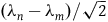 $(\lambda_n-\lambda_m)/\sqrt{2}$
; for instance, one could either add
 $(\lambda_n-\lambda_m)\theta_m{\psi}_m/\sqrt{2}$
or subtract
 $(\lambda_n-\lambda_m)\theta_n{\psi}_n/\sqrt{2}$
. That is to say, by (5) – namely the supposition that
 $\Psi$
is an eigenstate – we have
 $\left|{\hat T_1}{1 \over {\sqrt 2 }}({\theta _m}{\psi _m} + {\theta _n}{\psi _n})\right| \approx {{{\lambda _n} - {\lambda _m}} \over {\sqrt 2 }}.$
But for any Hermitian operator and normalized vector,
 $|\hat O\phi|$
cannot exceed the greatest eigenvalue. So in this case, by Heavy,
 $\left|{\hat T_1}{1 \over {\sqrt 2}}({\theta _m}{{\psi} _m} + {\theta _n}{{{\psi} _n})}\right| \le T_1^{\max } \ll {{{\lambda _n} - {\lambda _m}} \over {\sqrt 2 }},$
a manifest contradiction. Hence, the supposition is false, and an eigenstate of total energy cannot be a sum of
 $\theta_a{\psi}_a$
, but has the product form
 $\hat H\Psi_a(x_1,x_2)\approx{\hat H}\theta_a(x_1)\psi_a(x_1,x_2) \approx E_a\theta_a(x_1)\psi_a(x_1,x_2).$
□
Put another way, such states (approximately) diagonalize the total Hamiltonian: there are no cross-terms for such states with different values of a. (Note that in this approach, despite its historical name, separability is not an independent ansatz, but rather the consequence of the Heavy ansatz.)
The derivation depends crucially on the choice of bases
 $\{{\psi}_a(x_1,x_2)\}$
for the expansion, so that Heavy can be applied; indeed, in other bases it will not be the case that one term dominates, so the molecular wavefunction will not be even approximately separable. That is the significance of the clamped Hamiltonian(s) in this explication of BO, not that any of them literally approximates or idealizes or replaces the true Hamiltonian. In this sense, clamping is entirely formal, and does not represent the nuclei of the target molecule as fixed. (The system of electrons moving in the Coulomb field of some fixed charges that it could represent is fictive and entirely distinct from a physical molecule.)
Derivation 2 (Adiabatic approximation from Heavy). Recall that the position representation of
 ${\hat T}_1$
has the form
 $\partial^2/\partial x_1^2$
:
 ${\hat T_1}{\theta _a}{{\psi} _a} \propto {{{\partial ^2}} \over {\partial x_1^2}}{\theta _a}{{\psi} _a} = {{{\partial ^2}{\theta _a}} \over {\partial x_1^2}} \cdot {{\psi} _a}\; + 2{{\partial {\theta _a}} \over {\partial {x_1}}} \cdot {{\partial {{\psi} _a}} \over {\partial {x_1}}} + {\theta _a} \cdot {{{\partial ^2}{{\psi} _a}} \over {\partial x_1^2}}.$
However,
 $\theta_a{\psi}_a$
diagonalizes both
 ${\hat T}_2 +{\hat W}$
using (2), and (approximately)
 ${\hat H}={\hat T}_1+{\hat T}_2 +{\hat W}$
from ( 8). Therefore it also (approximately) diagonalizes
 ${\hat T}_1$
:
 $\langle\theta_b{\psi}_b |\hat T_1|\theta_a{\psi}_a\rangle\propto{\delta}_{a,b}$
. In the x-representation,
 $\int {\rm{d}} {x_1}\theta _b^*({x_1})\int {\rm{d}} {x_2}{\psi} _b^*({x_1},{x_2})\left\{ {{{\partial ^2}{\theta _a}} \over {\partial x_1^2}}{{\psi} _a}\; + 2{{\partial {\theta _a}} \over {\partial {x_1}}}{{\partial {{\psi} _a}} \over {\partial {x_1}}} + {\theta _a}{{{\partial ^2}{{\psi} _a}} \over {\partial x_1^2}}\right\} \propto {{\delta} _{a,b}}.$
Since different
 ${\psi}_a$
are orthogonal (since distinct eigenstates) the
 $x_2$
integral means that the first term in the sum is proportional to
 ${\delta}_{a,b}$
. However, neither of the derivatives of
 $\psi_a$
will be orthogonal to
 ${\psi}_b$
(and similarly for the
 $\theta$
s), so that the remaining terms will not be proportional to
 ${\delta}_{a,b}$
– unless they are both zero. Thus, ( 10) entails that
 ${{\partial {{\psi} _a}({x_1},{x_2})} \over {\partial {x_1}}} \approx 0$
(which is the more specific statement that often goes under the name of ‘Born–Oppenheimer approximation’). □
Note that (11) is ‘adiabatic’ in the sense that
 ${\psi}$
changes ‘slowly’ with respect to
 $x_1$
, not time (cf. Huggett and Thébault Reference Huggett and Thébault2023).
Let us repeat, for emphasis, the important features of this mathematical discussion. First, although the ratio of electron to neutron mass is relevant, it only provides an inequality, without taking any limit (and in any case merely motivates an ansatz). Second, at no point does one approximate the molecule as having ‘clamped’ nuclei; the role of (2) is to define a convenient basis in which an exact formal expansion can be made. As we have just seen, the crucial property of the basis is that – because of the mass ratio – one term in the expansion dominates for certain energy eigenstates of the molecule – nothing more. Third, every step of the derivations is fully quantum. And finally, they suffice to show the mathematically validity of the BO approximation (in cases in which the Heavy ansatz is correct).Footnote 21
That is, making the adiabatic approximation (11) in (9) yields
 ${{\hat T}_1}{\theta _a}{{\psi} _a} \approx {{\psi} _a}{{{\partial ^2}{\theta _a}} \over {\partial x_1^2}} = {{\psi} _a}{\hat T_1}{\theta _a}.$
In this specific sense, the part of the joint state
 $\Psi_a(x_1,x_2)$
that expresses the kinetic energy of the nuclei can (approximately) be factored out as
 $\theta_a(x_1)$
. But to repeat the discussion after (3), it cannot be over-emphasized that
 $\Psi_a(x_1,x_2)$
has not been factored into strictly nuclear and electronic parts, since the other factor,
 ${\psi}_a(x_1,x_2)$
, depends on both, not just the electron configuration.
Then, from (8), one needs to find
 $\theta_a(x_1)$
and
 ${\psi}_a(x_1,x_2)$
; the latter is given by (2), so all we need is the equation for the former. From (8) we have
 $({{\hat T}_1} + {{\hat T}_2} + {\hat W}){\theta _a}({x_1}){{\psi} _a}({x_1},{x_2}) \approx {{E}_a}{\theta _a}({x_1}){{\psi} _a}({x_1},{x_2}),$
while from (2) and (12) we have
 $ \approx ({{\hat T}_1}{\theta _a}({x_1})) \cdot {{\psi} _a}({x_1},{x_2}) + {\lambda _a}({x_1}){\theta _a}({x_1}){{\psi} _a}({x_1},{x_2}),$
which gives
 $({{\hat T}_1} + {\lambda _a}({x_1}) - {E_a}){\theta _a}({x_1}) \approx 0.$
This has the form of a (time-independent) Schrödinger equation for the nuclear variables, ‘living’ on a PES
 $\lambda_a(x_1)$
, but recall the discussion after (12). That cannot be the correct literal description of the nuclei in BO, since both
 $\theta_a(x_1)$
and
 ${\psi}_a(x_1,x_2)$
represent aspects of the nuclear subsystem.
To sum up, from the Born–Oppenheimer separation ansatz (8), finding the approximate eigenstates
 $\Psi(x_1,x_2)$
of
 $\hat H$
reduces to finding solutions to (2) and (15), and taking their product, a significant simplification. (Of course, these equations can still not be solved analytically, and require further approximations, for instance the WKB approximation.) Together these steps constitute BO, and as we have shown, if Heavy is true then they are fully quantum. Of course, as we have explained, making that ansatz is only valid if the results are (approximate) solutions in which Heavy holds; since they are, BO is fully quantum.
3.4. Quantum representation and the uncertainty principle
In the light of the textbook treatment it should be apparent why the quoted claims about violations of Heisenberg uncertainty are inconsistent with the representational structure of BO. The crucial assumption Heavy involves no conflict with or suspension of the Heisenberg uncertainty principle. Furthermore, a violation of the Heisenberg uncertainty principle is formally precluded by the definition of the objects that are playing representational roles within BO.
Heavy is entirely consistent with the principles of quantum theory, including Heisenberg’s. Indeed, the previous discussion makes clear that BO presupposes the standard wavefunction–observable representational structure of quantum theory, and hence entails the uncertainty relations. First, wavefunctions are square-integrable functions on (configuration) space
 ${L}^2(\mathbb{R}^n)$
. Second, (for a single degree of freedom) the variances of position and momentum variables are
 $\sigma_{x}^{2}=\int_{-\infty}^{\infty}x^{2}\cdot|{\psi} (x)|^{2}\,{\rm d}x$
and
 $\sigma_{p}^{2}=\int_{-\infty}^{\infty}p^{2}\cdot|\tilde{{\psi}}(p)|^{2}\,{\rm d}p$
, where
 ${\psi} (x)$
and
 $\tilde{{\psi}} (p)$
are the position and momentum basis wavefunctions, respectively. As is well known, the Heisenberg uncertainty relation,
 $ \sigma _{x} \sigma _{p} \geq \hbar/{2}$
, is then a simple mathematical consequence of the fact that position and momentum are Fourier conjugates.
A violation of the relation would require a ‘wavefunction’ sharply peaked in both the position and momentum basis simultaneously, contrary to this basic fact about quantum mechanics and BO. They would only be violated if the model represented electron or nuclei states as other than vectors in Hilbert space, say as delta functions in both position and momentum space.Footnote
22
Similarly, that the ‘nuclear wavefunction’
 $\theta_a(x_1)\in L^2(\mathbb{R}^m)$
is a vector in a Hilbert space means that it cannot violate the Heisenberg uncertainty relation; it does not and cannot violate the Heisenberg uncertainty relation. Moreover, as already noted, there is no justification for interpreting
 $\Psi_a(x_1,x_2)$
as factored into strictly nuclear and electronic parts. The factor,
 ${\psi}_a(x_1,x_2)$
, depends on the nuclear configuration, not just the electron configuration (hence the scare quotes around ‘nuclear wavefunction’). The role of ‘classical’ parameters and the ‘clamped’ Hamiltonian in constructing
 $\psi_a(x_1,x_2)$
is not relevant to the status of the nuclei as quantum particles since all the representation of states is via vectors in a Hilbert space.
The crucial point is that BO provides an inherently quantum representation of molecular structure that does not admit a classical separation into purely electronic and nuclear representations. The quantum nature of the nuclei in the BO is highlighted in the discussion of Jecko (Reference Jecko2014) who notes in his concluding section: ‘We emphasise that, in the mathematical treatment of the Born–Oppenheimer approximation, the nuclei are always considered as quantum particles. The use of clamped nuclei is just a tool to construct an appropriate effective Hamiltonian but the latter is a quantum, nuclear Hamiltonian with restricted electronic degrees of freedom’ Jecko (Reference Jecko2014), p. 20. We will return to the quantum status of BO in the context of our more mathematically rigorous treatment in the next section.
4. On the mathematical treatment of Born–Oppenheimer
Our explication of BO was, as we have explained, at a textbook level, eliding details and rigour for the sake of the larger mathematical picture. In this section we will discuss certain salient details, while still leaving others to the mathematical literature. In particular, there is an issue raised by Sutcliffe and Woolley (Reference Sutcliffe and Guy Woolley2012); Sutcliffe and Woolley (Reference Sutcliffe, Guy Woolley, Hotokka, Brändas, Maruani and Delgado-Barrio2013) (and elsewhere in their work), critiquing Born and Huang (Reference Born and Huang1954), sometimes cited in support of the philosophical literature that we have criticized.
Sutcliffe and Woolley (Reference Sutcliffe, Guy Woolley, Hotokka, Brändas, Maruani and Delgado-Barrio2013) point out that the part of the total molecular Hamiltonian (1) containing the contributions from electronic kinetic energy and total Coulomb potential energy,
 ${\hat T}_2+{\hat W}$
, which they denote
 ${\hat H}^{{\rm elec}}$
, has a continuous spectrum (pp. 18–20). (Because, they argue,
 ${\hat H}^{{\rm elec}}$
is the direct integral of the
 $x_1$
-parameterized family of clamped Hamiltonians,
 ${\hat T}_2+{\hat W}(x_1)$
.) Of course, this fact is consistent with the discrete spectrum of the full Hamiltonian. However, it implies that (a) the PESs cannot be understood as representing the spectrum of
 ${\hat H}^{{\rm elec}}$
, since they are discrete, and (b) BO cannot be understood as a perturbation of
 ${\hat H}^{\mathrm{elec}}$
, with small corrections due to nuclear motion: they could not make the spectrum discrete (also,
 ${\hat H}^{{\rm elec}}$
gives no PESs for finding a nuclear perturbation).
Sutcliffe and Woolley give as their target a common story about BO that holds the contrary view concerning these points, and their refutation is convincing. However, it does not appear to cause any difficulties for our explication. (a) The PESs are defined by the individual members of the parameterized family of clamped Hamiltonians, not by their direct integral,
 ${\hat H}^{{\rm elec}}$
; speaking extremely loosely, they are the ‘direct integral’ of their eigenvalues, not the eigenvalues of their direct integral. (b)
 ${\hat H}^{{\rm elec}}$
, as opposed (again) to the family of clamped Hamiltonians, plays no role in our exposition, which therefore certainly does not represent the BO as a perturbation about it! Indeed, Sutcliffe and Woolley (Reference Sutcliffe, Guy Woolley, Hotokka, Brändas, Maruani and Delgado-Barrio2013), p. 28 seems to agree that a proper formulation of BO in the kind of terms we have described allows ‘a rigorous account of the separation of electronic and nuclear motion’.
Regarding (a), note that the derivation itself shows why the PESs are relevant to BO: we have seen that they are precisely the functions that appear, as a matter of mathematics, as potential terms in (15). No more explanation is needed, and no need to think of any literal clamping occurring. Of course, the role of the PES is much richer than this in quantum chemistry, and far more can be said about its general physical significance (something we touch on in section 5). Again, this paper is focused specifically on BO, not on chemistry in general, though of course we postulate that the kind of analysis presented can be generalized.
Jecko (Reference Jecko2014) invokes Sutcliffe and Woolley’s arguments and ‘slightly pessimistic note’, to review the current state of mathematical knowledge regarding BO and, specifically, to explain, more optimistically, how mathematical physicists have dealt with a distinct issue regarding continuous spectra.Footnote 23 The problem is that the ‘clamped’ Hamiltonians used in BO generally have a continuous part to their spectra (representing energies at which the constituents have disassociated, and there is no longer a stable molecule), above the discrete part (corresponding to a bound state). Our analysis assumed that the spectra are purely discrete – the existence of a PES depends on it – so it is crucial to our interpretive claims to understand the nature and justification of this assumption. Indeed, Jecko’s discussion identifies three principal problems for making the textbook treatment of BO exact, each of which we should address.Footnote 24
First, the analysis only involves the internal energy of the molecule, even though it has centre-of-mass motion and associated kinetic energy, with a continuous spectrum (absent boundary conditions). To separate out the internal levels (to find the spectrum, or the spatial structure, or for scattering) one can transform to a centre-of-mass frame (of the molecule or just its nuclei, depending on the problem), and subtract the centre-of-mass kinetic energy. This procedure introduces a new term into the Hamiltonian (the Hughes–Eckart energy), which is suppressed by the ratio of electronic to nuclear masses (
 $\sim10^{-3}$
), so is neglected in low-order approximation.Footnote
25
This complication is harmless for present purposes, so we suppressed it for reasons of space.
The second problem arises because the expansion (3) is not really a sum, but a sum of low-energy states plus an integral over states in the high-energy, continuous part of the spectrum of
 $\hat T_2+\hat W$
. As is familiar, in any continuous spectrum there are no normalizable eigenstates, something finessed in familiar ways by physicists via the Dirac delta function, and more rigorously by the theory of ‘spectral decomposition’. However, in the present case details of the structure of the spectrum, in particular the existence of ‘thresholds’, Jecko (Reference Jecko2014),
 ${\rm{\S}}$
V, make the expansion highly non-trivial, and hard to control mathematically, due to the possibility of divergences at the thresholds. Its existence is thus – from a mathematically rigorous point of view – an ‘in principle’ matter only.
The third ‘problem’ is that the appropriate formalism for a mathematically rigorous treatment is, as discussed earlier, that of the direct integral (Reed and Simon Reference Reed and Simon1978, pp. 280–87). Any
 ${L}^2(\mathbb{R}^m\times\mathbb{R}^n)$
function
 $f(x_1,x_2)$
is understood as an
 $L^2(\mathbb{R}^n)$
-valued function
 $f(x_1,\cdot)$
with
 $x_1\in\mathbb{R}^m$
. One then naturally defines the direct integral of a parameterized family of operators
 $\hat O(x_1)$
on
 $L^2(\mathbb{R}^n)$
as the operator
 $\hat O$
on
 $L^2(\mathbb{R}^m\times\mathbb{R}^n)$
whose effect on
 $f(x_1,x_2)$
is the direct integral of
 $\hat O(x_1)f(x_1,\cdot)$
; i.e., it acts on each
 $x_2$
function as the appropriate operator in its state space.Footnote
26
So one needs to be sure that the formalism is respected.
In response to the last two problems, mathematical physicists have a somewhat different perspective on BO to that of section 3.2.Footnote
27
The goal is to approximate an eigenstate (and eigenvalue) lying in the low-energy, discrete part of the spectrum of the molecule (1). To do this, one considers eigenstates of the Hamiltonian projected onto the subspace in which its spectrum is discrete. See Jecko (Reference Jecko2014),
 ${\rm{\S}}$
IV for details of the following sketch.
As noted,
 ${\hat T}_2+{\hat W}$
is the direct integral of the clamped Hamiltonians
 ${\hat T}_2+{\hat W}(x_1)$
. While the latter act on
 ${L}^2(\mathbb{R}^n)$
, the state space of the electron subsystem, the former acts on
 ${L}^2(\mathbb{R}^m\times\mathbb{R}^n)$
, the state space of the full system, including both the electrons and the nuclei; both, that is, are quantum mechanical.
 ${\hat T}_2+{\hat W}$
is also often called the ‘electronic Hamiltonian’ (e.g.,
 ${\hat H}^{{\rm elec}}$
above), but that would be misleading for current purposes since it acts on the state of the whole molecule. Similarly for projection operators: for a given
 $x_1=X$
and eigenstates
 ${\psi}_a(X; x_2)$
of
 ${\hat T}_2+{\hat W}(X)$
lying in a finite discrete part of its spectrum there is an operator
 ${\hat P}(X)f({x_2}) = \sum\limits_{a = 1}^N {{{\psi} _a}} (X;{x_2})\int {{\psi} _a^*} (X;{x'_2})f({x'_2}){\rm{d}}{x'_2} \equiv \sum\limits_{a = 1}^N {{\phi _a}} (X) \cdot {\psi _a}(X;{x_2})$
projecting
 $f(x_2)\in {L}^2(\mathbb{R}^n)$
onto the subspace spanned by the
 ${\psi}_a(X; x_2)$
. Then,
 $\hat P$
, the direct integral of the
 ${\hat P}(x_1)$
projects states in
 $L^2(\mathbb{R}^m\times\mathbb{R}^n)$
onto the proper subspace, V, spanned by the direct products of the
 $\phi(X){\psi}_a(X; x_2)$
. Since
 $\hat P$
also acts on the full molecular state space, it too treats both nuclei and electrons as quantum mechanical.
To overcome the issue of the continuous part of the clamped Hamiltonian’s spectrum, the approximation made – see Jecko (Reference Jecko2014,
 ${\rm{\S}}$
IV) for justification – is to seek eigenstates for the projected molecular Hamiltonian
 ${\hat H}_{\text{eff}}={\hat P}({\hat T}_1+{\hat T}_2+{\hat W}){\hat P}$
, instead of for
 ${\hat T}_1+{\hat T}_2+{\hat W}$
. One assumes that if an eigenstate of the latter exists in a given narrow range of the energy, then it can be approximated by an eigenstate of the former lying in the same range: one replaces the tricky problem of solving the ‘true’ Hamiltonian with the simpler problem of solving an effective Hamiltonian for the energy range of a stable molecule. Formally,
 ${\hat H}_{\text{eff}}$
acts on
 ${L}^2(\mathbb{R}^m\times\mathbb{R}^n)$
: first a state is projected onto V, then acted on by the molecular Hamiltonian, and the result projected again onto the subspace.
 ${\hat H}_{\text{eff}}$
too treats both nuclei and electrons as quantum. Note that the effect of
 ${\hat H}_{\text{eff}}$
is always to produce a vector in V, so while (a) all states orthogonal to V are eigenstates of
 ${\hat H}_{\text{eff}}$
with eigenvalue 0, (b) all its other eigenstates lie in V.Footnote
28
The upshot is, in relation to sections 3.2 and 3.3, that by excising the continuous part of the spectra, one has made rigorous (3), now understood as expanding solutions of the Schrödinger equation for the projected Hamiltonian, within the defined energy range.
The previous sections show that textbook BO is fully quantum, and adding a step in which the Hamiltonian is projected onto a subspace of the Hilbert space in no way undermines that argument. The projected Hamiltonian is still quantum, indeed a quantum theoretical approximation to the quantum Hamiltonian. The difference is rather that BO is no longer understood as the lowest order in some well-defined exact expansion, but rather as an approximation, with some well-understood corrections, to an exact solution. This situation is in contrast, not only to our textbook-style presentation, but also to those of Born and Oppenheimer, Born and Huang, and Messiah; while more careful than ours, theirs remain heuristic.Footnote 29 Once the appropriate formal machinery has been deployed, BO can be formalised to the standards of rigour of mathematical physics. No assumptions inconsistent with quantum theory are involved.
5. Rigour and reduction in quantum chemistry
This final section considers questions of mathematical rigour and reduction in quantum chemistry more generally. Let us start with the role of ‘classical’ assumptions in the emergence of ‘determinate molecular structure’. Let us first assume that what is meant by ‘determinate molecular structure’ is provided by the regime in which the adiabatic approximation is valid, and thus the nuclei are such that the variation of the ‘electron’ wavefunction with respect to nuclear positions is approximately zero. Sections 3 and 4 show exhaustively that the emergence of such structure requires neither classical assumptions in the sense of clamped nuclei, nor violation of the uncertainty relation. Rather, the assumption required for BO is Heavy, which is entirely consistent with a fully quantum treatment of the molecule. There is a richer notion of molecular structure that includes the number, angles, and lengths of chemical bonds and chirality (Franklin and Seifert Reference Franklin and Seifert2024). BO is far from sufficient to model such structure, although plausibly in some circumstances it may prove necessary.Footnote 30 In this context, there is debate about the requirement for a solution to the measurement problem of quantum theory in order to account for the emergence of molecular structure (Franklin and Seifert Reference Franklin and Seifert2024; Fortin and Lombardi Reference Fortin and Lombardi2021; Seifert Reference Seifert, Lombardi, González and Fortin2022; Miller Reference Miller2023). However, it remains to be seen which foundational features, if any, mark out a particular distinctiveness of quantum chemistry, within the vast array of applications of quantum mechanics to diverse matter systems, including non-molecular states of matter such as plasmas or Bose–Einstein condensates.
More generally, in the context of discussions of ‘classical’ and ‘semi-classical’ assumptions our positive proposal for precise scientific language use is as follows. Firstly, models such as BO should be described as ‘quantum’ models of molecules, since all aspects of the molecules are treated quantum mechanically within the Hilbert space formalism. This is not withstanding the fact that BO can be understood as ‘mimicking’ a semiclassical Schrödinger operator due to the functional analogy between the the nuclear kinetic energy term and a semiclassical Laplace operator Jecko (Reference Jecko2014), p. 19. Furthermore, on this proposed usage adiabaticity is neither necessary nor sufficient for semi-classicality. Quantum models can be adiabatic and semi-classical models can be non-adiabatic.
Secondly, one may legitimately deploy the term ‘semi-classical’ in a broad sense to indicate an application of quantum theory in which, while the system is treated quantum mechanically, the model includes radiative fields that are not. In this sense, the original quantum theory of the atom, as well as the modern quantum-mechanical treatment, is ‘semi-classical’ since the electromagnetic field through which the nucleus and the electrons interact is not quantized (cf. Boucher and Traschen Reference Boucher and Traschen1988). Similarly for most of quantum chemistry including BO. It would be moot to claim that chemistry does not reduce to quantum physics because the physics in question is semi-classical in this sense, because huge amounts of what is ordinarily called ‘quantum physics’ is! (For example, standard non-relativistic quantum mechanics other than free particles, including most condensed matter physics.) Such semi-classical physics is a kind of quantum physics.
Thirdly, one should distinguish various more specific meanings of ‘semi-classical’. One refers to a quantum mechanical expansion, in terms of classical zeroth order plus quantum corrections, which is truncated at some order in
 $\hbar$
(or other parameter such as mass ratios) to provide an approximate model.Footnote
31
In such cases, the semi-classical model is a sub-model within the general framework of quantum theory.Footnote
32
A formally closely related, but physically and conceptually different, sense of ‘semi-classical’ is found in the context of certain ‘semi-classical’ approaches to gravity where the field equations are re-written in terms of classical metric variables on the left-hand side but the first moment (i.e., expectation value) of the stress–energy tensor is inserted on the right-hand side. A further notion of semi-classicality refers to specific behaviour in the limit (usually
 $\hbar\rightarrow0$
) in which the classical theory obtains.Footnote
33
Finally, the term ‘semi-classical’ is applied to mixed classical-quantum models which simultaneously feature representations of classical and quantum states and dynamics. The former in terms of classical phase space states and Poisson bracket structure, and the latter in terms of operators, density matrices, and commutator brackets structure. Mixed classical-quantum models have been widely applied in non-adiabatic quantum chemical modelling (Tully Reference Tully1991; Crespo-Otero and Barbatti Reference Crespo-Otero and Barbatti2018) and bring up various interesting issues that are worthy of philosophical engagement.
It is useful to distinguish the distinct modelling contexts in which semi-classical models, in one or more of the more specific senses, might be deployed within quantum chemistry and articulate the relevance for reductive explanations in each context. They are as follows. (i) Mathematical idealization: The model is being used to represent fully quantum phenomena and the semi-classical features are a mathematical idealization that relates the semi-classical effective model to a (less) idealized fully quantum model. Given the stability of salient explanatory features under de-idealization, there is no potential problem for reductive explanations of the relevant phenomena. (ii) Physical idealization: The model is being used to represent fully quantum phenomena but this representation is via a proxy model of semi-classical phenomena that approximate the quantum phenomena for the purposes and degree of accuracy required. Again, there is no problem for reductive explanations given stability of the salient explanatory features under de-idealization (Bokulich Reference Bokulich2008; Bokulich Reference Bokulich, Magnani and Bertolotti2017). (iii) Emergent phenomena: The model is being used to represent emergent semi-classical phenomena that occur in the context of classical-quantum limit behaviour. There is a putative problem for any account of reductive explanation that is incompatible with emergence qua novel and robust behaviour, but not for any account of reductive explanation that is so compatible (cf. Bokulich Reference Bokulich2008; Butterfield Reference Butterfield2011; Franklin Reference Franklin2024).
A further issue is the role of the environment (Ladyman and Thébault Reference Ladyman and Thébault2024). In this context, Sutcliffe and Woolley (Reference Sutcliffe and Guy Woolley2012) say ‘one should not expect useful contact between the quantum theory of an isolated molecule and a quantum account of individual molecules, as met in ordinary chemical situations where persistent interactions (due to the quantized electromagnetic field, other molecules in bulk media) and finite temperatures are the norm’ (p. 7). These remarks, together with related ideas developed by Seifert (Reference Seifert, Lombardi, González and Fortin2022), form a fruitful basis for an ‘open systems view’ of quantum chemistry in the manner recently proposed for quantum physics more generally by Cuffaro and Hartmann (Reference Cuffaro and Hartmann2021). We expect that such a view would prove to be consistent with any suitably nuanced model-based understanding of reduction and idealization.Footnote 34
We conclude with the following questions. Is there a methodological distinction between the use of models in modern quantum chemistry, and other examples of quantum modelling practice in matter systems, such as applications of quantum mechanics to solid state or few body systems? Is there space for distinctively ‘chemical’ modes of quantum modelling practice? In answering such questions we suggest that philosophers need to re-conceptualize the physics–chemistry interface and move beyond the confines of the reduction vs. anti-reduction dialectic. Plausibly, the characteristically ‘chemical’ aspects of quantum chemistry are rooted in methodology rather than disparate formal features of the models;Footnote 35 for example, experimental practices, such as spectroscopy. On our view, we should understand quantum chemistry as neither a putative case of inconsistency between chemistry and physics nor an instance of subsumption of the former by the latter. The field of quantum chemistry should not be understood to mark a boundary between the distinctly chemical and distinctly physical, nor, moreover, between classical and quantum modes in the representations of molecules.Footnote 36 Rather, quantum chemistry should be recast as a ‘littoral zone’ with its own distinctive modelling ecology, conditioned by its role as the fertile meeting place of the two disciplines.
Acknowledgements
Thanks to Hernán Accorinti, Guido Bacciagaluppi, Hasok Chang, Sebastian Fortin, Robin Hendry, Juan Camilo Martínez González, Olimpia Lombardi, Vanessa Seifert, Guy Woolley, Nick Norman, Fred Manby two anonymous referees, and audiences at several venues for responses to and discussions of drafts, which helped us sharpen our arguments, and avoid some errors. Thanks especially to Thierry Jecko for generous discussion and feedback.
Funding statement
This work was supported by the Benjamin Meaker Fellowship programme at the University of Bristol and by John Templeton Foundation grant number 62210.
Declarations
None.


 λn
 x1
 x1=x

 Open access

