

1 Introduction
Combined turbulent thermal convection and magnetic fields significantly affect the flow structure and transport of momentum and heat in electrically conducting fluids. The effect plays an important role in numerous systems found in technology and nature (Ozoe Reference Ozoe2005; Weiss & Proctor Reference Weiss and Proctor2014; Davidson Reference Davidson2016). Prominent technological examples are liquid-metal batteries, the growth of semiconductor crystals, and the design of blankets and divertors in nuclear fusion reactors. A notable example of a natural system is the planetary dynamo. We consider the basic configuration of Rayleigh–Bénard convection (RBC) in a cylinder with thermally insulating sidewalls and an imposed vertical magnetic field. The quasi-static approximation of low magnetic Reynolds numbers  $Re_{m}\ll 1$ and Prandtl numbers
 $P_{m}\ll 1$ typical for laboratory experiments and industrial processes with liquid-metal flows is utilized to describe the electromagnetic interactions. This implies that the applied magnetic field
 $\boldsymbol{B}_{0}$ is much stronger than the induced one
 $\boldsymbol{b}$ (Davidson Reference Davidson2016). The induced magnetic field is neglected in the expressions for the Lorentz force and Ohm’s law. Furthermore, the induced field is assumed to adjust instantaneously to changes of velocity. The flow–field interaction is, essentially, approximated as a one-way influence of the magnetic field on the flow.
The effect of a vertical magnetic field on RBC has been studied experimentally (Nakagawa Reference Nakagawa1957; Cioni, Chaumat & Sommeria Reference Cioni, Chaumat and Sommeria2000; Aurnou & Olson Reference Aurnou and Olson2001; Burr & Müller Reference Burr and Müller2001; King & Aurnou Reference King and Aurnou2015; Zürner et al. Reference Zürner, Schindler, Vogt, Eckert and Schumacher2020), numerically (Liu, Krasnov & Schumacher Reference Liu, Krasnov and Schumacher2018; Yan et al. Reference Yan, Calkins, Maffei, Julien, Tobias and Marti2019; Akhmedagaev et al. Reference Akhmedagaev, Zikanov, Krasnov and Schumacher2020) and theoretically (Chandrasekhar Reference Chandrasekhar1961; Houchens, Witkowski & Walker Reference Houchens, Witkowski and Walker2002; Busse Reference Busse2008). The dynamics of the system is determined by three dimensionless control parameters: the Rayleigh, Hartmann and Prandtl numbers given by
 $$\begin{eqnarray}Ra=\frac{g\unicode[STIX]{x1D6FC}\unicode[STIX]{x0394}TH^{3}}{\unicode[STIX]{x1D708}\unicode[STIX]{x1D705}},\quad Ha=B_{0}H\sqrt{\frac{\unicode[STIX]{x1D70E}}{\unicode[STIX]{x1D70C}\unicode[STIX]{x1D708}}}\quad \text{and}\quad Pr=\frac{\unicode[STIX]{x1D708}}{\unicode[STIX]{x1D705}},\end{eqnarray}$$
with the acceleration due to gravity  $g$, the thermal expansion coefficient
 $\unicode[STIX]{x1D6FC}$, the temperature difference between the horizontal boundaries of the fluid layer
 $\unicode[STIX]{x0394}T$, the height of the layer
 $H$, the kinematic viscosity
 $\unicode[STIX]{x1D708}$, the temperature diffusivity
 $\unicode[STIX]{x1D705}$, the electrical conductivity
 $\unicode[STIX]{x1D70E}$, the mass density
 $\unicode[STIX]{x1D70C}$ and the magnetic permeability of free space
 $\unicode[STIX]{x1D707}_{0}$. Systems with lateral walls add the aspect ratio
 $\unicode[STIX]{x1D6E4}=D/H$ as a parameter, where
 $D$ is the typical horizontal size, the diameter of the cylinder in our case.
The classical picture of the effect of a magnetic field on RBC in an infinite horizontal layer includes suppression of turbulence (Nakagawa Reference Nakagawa1957) and increase of the critical Rayleigh number  $Ra_{c}$ for the onset of convection. The latter effect is given by Chandrasekhar (Reference Chandrasekhar1961) in the asymptotic form at high
 $Ha$ as
 $Ra_{c}\approx \unicode[STIX]{x03C0}^{2}Ha^{2}$. The dominance of quasi-two-dimensional (Q2D) cellular and columnar structures in the flows at
 $Ra>Ra_{c}$ within a layer with stress-free boundary conditions was observed by Yan et al. (Reference Yan, Calkins, Maffei, Julien, Tobias and Marti2019). These regimes are uniquely identified by the slope of the Nusselt number
 $Nu(Ra)$ and Reynolds number
 $Re(Ra)$, the physical structure of the flows, and the relative sizes of terms in the governing equations. The flow regimes are identified as Q2D when the velocity and temperature fields are virtually independent of the axial direction outside of the boundary layers near the top and bottom walls.
The theoretical analysis of Busse (Reference Busse2008) predicts that the presence of the sidewalls leads to the onset of convection at a much lower  $Ra$ than in an infinite layer. The heat transfer in that case is concentrated near the walls. Recent numerical simulations (Liu et al. Reference Liu, Krasnov and Schumacher2018) of RBC in a rectangular cell at
 $Ra\sim Ra_{c}$ and
 $Ra<Ra_{c}$ confirmed the existence of this so-called wall-mode regime, in which significant flow and heat transfer are limited to narrow zones near the sidewalls (the wall modes). These modes are planar jets at moderate
 $Ha$, but have a complex two-layer structure at high Hartmann numbers, higher than
 $Ha_{c}\equiv \sqrt{Ra}/\unicode[STIX]{x03C0}\approx 1000$. Wall modes have also been found in simulations of RBC in a cylindrical cell at
 $\unicode[STIX]{x1D6E4}=4$,
 $Pr=0.025$,
 $Ha\leqslant 1000$ and
 $Ra=10^{7}$ (Akhmedagaev et al. Reference Akhmedagaev, Zikanov, Krasnov and Schumacher2020). The simulation results are consistent with the recent extensive measurements of RBC with a vertical magnetic field in a cylinder with moderate
 $Ra$ and
 $Ha$ by Zürner et al. (Reference Zürner, Schindler, Vogt, Eckert and Schumacher2019, Reference Zürner, Schindler, Vogt, Eckert and Schumacher2020).
We should also mention a certain similarity between the behaviour found in RBC with a vertical magnetic field and that in convection with rotation around a vertical axis. The formation of Q2D structures, faster growth of heat transfer rate with  $Ra$ at high rotation rates, and wall modes are observed in rotating systems (Zhong, Ecke & Steinberg Reference Zhong, Ecke and Steinberg1991; Ecke, Zhong & Knobloch Reference Ecke, Zhong and Knobloch1992; Zhang et al. Reference Zhang, van Gils, Horn, Wedi, Zwirner, Ahlers, Ecke, Weiss, Bodenschatz and Shishkina2019).
The focus of our investigation here is on the RBC with a vertical magnetic field and sidewalls at  $Ra\gg Ra_{c}$. High-resolution direct numerical simulations (DNS) of flows in a cylindrical cavity with
 $\unicode[STIX]{x1D6E4}=1$,
 $Pr=0.025$,
 $10^{7}\leqslant Ra\leqslant 10^{9}$ and
 $0\leqslant Ha\leqslant 1400$ are performed. The work follows the experiments by Cioni et al. (Reference Cioni, Chaumat and Sommeria2000) carried out at the same
 $\unicode[STIX]{x1D6E4}$ and
 $Pr$ (mercury) and at
 $Ra\leqslant 3\times 10^{9}$ and
 $Ha\leqslant 2000$ (the highest
 $Ra$ and
 $Ha$ achieved so far). The experiments have shown that the slope
 $\unicode[STIX]{x1D6FD}$ of the asymptotic power law
 $Nu\sim Ra^{\unicode[STIX]{x1D6FD}}$ increases from
 $\unicode[STIX]{x1D6FD}\approx 0.26$ in non-magnetic flows to up to
 $\unicode[STIX]{x1D6FD}\approx 1$ at high
 $Ha$. The result is that the heat transfer rate in high-
 $Ra$ flows in very strong magnetic fields becomes comparable to the rate in turbulent flows without the magnetic field. The physical mechanisms determining this behaviour remain uncertain.
To the best of our knowledge, this study is the first to analyse turbulent RBC at high  $Ha$ and realistically low
 $Pr$ in the framework of high resolution DNS. The only related simulations have been performed by Lim et al. (Reference Lim, Chong, Ding and Xia2019) in a cubic convection cell at unrealistic
 $Pr=8$ with
 $Ra$ up to
 $10^{10}$ and
 $Ha$ up to
 $800$.
2 Presentation of the problem
2.1 Physical model
We consider the flow of an incompressible, viscous, electrically conducting fluid (a liquid metal) with constant physical properties contained in a cylinder with a uniform axial magnetic field. The governing equations are made dimensionless by using the cylinder’s height  $H$, the free-fall velocity
 $U=\sqrt{g\unicode[STIX]{x1D6FC}\unicode[STIX]{x0394}TH}$, the external magnetic field strength
 $B_{0}$ and the imposed temperature difference
 $\unicode[STIX]{x0394}T=T_{bottom}-T_{top}$ as the scales of length, velocity, magnetic field and temperature, respectively. The Boussinesq and quasi-static approximations are used. The equations are
 $$\begin{eqnarray}\displaystyle & \displaystyle \unicode[STIX]{x1D735}\boldsymbol{\cdot }\boldsymbol{u}=0, & \displaystyle\end{eqnarray}$$
 $$\begin{eqnarray}\displaystyle & \displaystyle \frac{\unicode[STIX]{x2202}\boldsymbol{u}}{\unicode[STIX]{x2202}t}+(\boldsymbol{u}\boldsymbol{\cdot }\unicode[STIX]{x1D735})\boldsymbol{u}=-\unicode[STIX]{x1D735}p+\sqrt{\frac{Pr}{Ra}}\left(\unicode[STIX]{x1D735}^{2}\boldsymbol{u}+Ha^{2}(\,\boldsymbol{j}\times \boldsymbol{e}_{z})\right)+T\boldsymbol{e}_{z}, & \displaystyle\end{eqnarray}$$
 $$\begin{eqnarray}\displaystyle & \displaystyle \frac{\unicode[STIX]{x2202}T}{\unicode[STIX]{x2202}t}+\boldsymbol{u}\boldsymbol{\cdot }\unicode[STIX]{x1D735}T=\sqrt{\frac{1}{RaPr}}\unicode[STIX]{x1D735}^{2}T, & \displaystyle\end{eqnarray}$$
 $$\begin{eqnarray}\displaystyle & \displaystyle \boldsymbol{j}=-\unicode[STIX]{x1D735}\unicode[STIX]{x1D719}+(\boldsymbol{u}\times \boldsymbol{e}_{z}), & \displaystyle\end{eqnarray}$$
 $$\begin{eqnarray}\displaystyle & \displaystyle \unicode[STIX]{x1D735}^{2}\unicode[STIX]{x1D719}=\unicode[STIX]{x1D735}\boldsymbol{\cdot }(\boldsymbol{u}\times \boldsymbol{e}_{z}), & \displaystyle\end{eqnarray}$$
where  $p$,
 $\boldsymbol{u}$,
 $\unicode[STIX]{x1D719}$ and
 $T$ are the fields of pressure, velocity, electric potential and deviation of temperature from a reference value. The top and bottom walls are maintained at constant temperatures
 $T=-0.5$ and
 $T=0.5$, respectively. The lateral wall is thermally insulated, so having
 $\unicode[STIX]{x2202}T/\unicode[STIX]{x2202}n=0$. No-slip boundary conditions for velocity are applied at the walls. All walls are perfectly electrically insulated, which implies
 $\unicode[STIX]{x2202}\unicode[STIX]{x1D719}/\unicode[STIX]{x2202}n=0$.
2.2 Numerical method
The governing equations (2.1)–(2.5) are solved numerically using the finite difference scheme described earlier by Krasnov, Zikanov & Boeck (Reference Krasnov, Zikanov and Boeck2011, Reference Krasnov, Zikanov and Boeck2012), Zhao & Zikanov (Reference Zhao and Zikanov2012) and Zikanov, Listratov & Sviridov (Reference Zikanov, Listratov and Sviridov2013). The performance of the method in applications to convection with a magnetic field was analysed in comparison with other methods, in particular with the finite-volume approach by Gelfgat & Zikanov (Reference Gelfgat and Zikanov2018). The spatial discretization is implemented in cylindrical coordinates with the boundary conditions at the axis specified as discussed by Zikanov et al. (Reference Zikanov, Listratov and Sviridov2013). The scheme is of the second order and nearly fully conservative with regards to the mass, momentum, kinetic energy and electric charge conservation principles (Krasnov et al. Reference Krasnov, Zikanov and Boeck2011; Ni et al. Reference Ni, Munipalli, Huang, Morley and Abdou2007). The time discretization is semi-implicit and based on the Adams–Bashforth/backward-differentiation method of the second order. Implicit treatment is applied to the diffusive term in (2.3) and the azimuthal derivative part of the Laplacian in (2.2). The radial and axial parts of the viscous term in (2.2) are treated explicitly. At every time step, three elliptic equations – the projection method equation for pressure, the equation for temperature and the potential equation (2.5) – are solved using the fast Fourier transform (FFT) in the azimuthal direction and the cyclic reduction solver in the  $r$–
 $z$ plane. The computational grid is clustered towards the walls according to the coordinate transformation in the axial direction
 $z=\tanh (A_{z}\unicode[STIX]{x1D701})/\tanh (A_{z})$ and in the radial direction
 $r=0.9\sin (\unicode[STIX]{x1D702}\unicode[STIX]{x03C0}/2)+0.1\unicode[STIX]{x1D702}$. Here
 $-1\leqslant \unicode[STIX]{x1D701}\leqslant 1$ and
 $0\leqslant \unicode[STIX]{x1D702}\leqslant 1$ are the virtual uniform coordinates, in which the grid is uniform. The novel features that appear in the new version of the algorithm and its thorough verification are presented by Akhmedagaev et al. (Reference Akhmedagaev, Zikanov, Krasnov and Schumacher2020).
All the results presented below are for the stage of a fully developed flow. The non-magnetic flows are taken as initial conditions for magneto-convection flows. Global transport properties of momentum and heat transfer are quantified by the Reynolds number  $Re=u_{rms}\sqrt{Ra/Pr}$ with root-mean-square velocity
 $u_{rms}=\langle u_{r}^{2}+u_{z}^{2}+u_{\unicode[STIX]{x1D703}}^{2}\rangle _{V,t}$ and the Nusselt number
 $Nu=1+\sqrt{RaPr}\langle u_{z}T\rangle _{V,t}$, where
 $\langle \cdot \rangle _{V,t}$ stands for volume and time averaging, respectively. The time averaging is performed over at least 100 convective time units.
2.3 Grid sensitivity study
The results of the grid sensitivity study are summarized in the supplementary material (available at https://doi.org/10.1017/jfm.2020.336). Verification of the model in comparison with experimental and numerical data is discussed in § 3.2. Here we briefly discuss the grid requirements and the grids used in our simulations. In addition to the internal structure of the flow, four boundary layers need to be accurately resolved (Grossmann & Lohse Reference Grossmann and Lohse2001; Davidson Reference Davidson2016): the thermal boundary layer of thickness  $\unicode[STIX]{x1D6FF}_{T}\approx 1/(2Nu)$, the viscous boundary layer with
 $\unicode[STIX]{x1D6FF}_{v}\approx 1/(4\sqrt{Re})$, the Shercliff layer with
 $\unicode[STIX]{x1D6FF}_{Sh}=1/\sqrt{Ha}$ at the lateral wall, and the Hartmann layer with
 $\unicode[STIX]{x1D6FF}_{Ha}=1/Ha$ at the top and bottom walls.
We find that grids with  $N=N_{r}\times N_{z}\times N_{\unicode[STIX]{x1D703}}=192^{3},256^{3}$ and
 $384^{3}$ and the clustering parameter
 $A_{z}=3.0$ are sufficient for non-magnetic flows at
 $10^{7}\leqslant Ra<10^{8}$,
 $10^{8}\leqslant Ra<10^{9}$ and
 $Ra=10^{9}$, respectively. Further refinement of the grid does not lead to significant changes. At the same time, the grid sensitivity study and the comparison between the maximum grid step in the bulk with the estimates of the Kolmogorov length scale indicate that the non-magnetic flow at
 $Ra=10^{9}$ is somewhat under-resolved. This is viewed as acceptable because the focus of our work is on flows at high Hartmann numbers.
Suppression of velocity gradients by the magnetic field allows us to alleviate the resolution requirements for the radial and azimuthal directions. Our study shows that  $N_{r}$ and
 $N_{\unicode[STIX]{x1D703}}$ not higher than
 $192$ and
 $256$ grid points are needed to accurately resolve flow structures at
 $Ha\geqslant 450$ with
 $10^{7}\leqslant Ra<10^{8}$ and
 $10^{8}\leqslant Ra\leqslant 10^{9}$, respectively. Considering the resolution along the axial coordinate, we need to take into account the Q2D character of the flow with weak axial gradients of velocity in the core (we must note that the gradients do not approach zero at high
 $Ra$ even at the strongest magnetic fields) and thin Hartmann boundary layers at the top and bottom walls. This allows us to rely on grids with the smaller number of points, but stronger near-wall clustering. The grid sensitivity study shows that, depending on the value of
 $Ha$,
 $N_{z}$ between
 $64$ and
 $256$ and
 $A_{z}$ between
 $3$ and
 $4$ securing not less than six points within the Hartmann layer are sufficient.
As presented in detail in the supplementary material, our simulations show good grid convergence for  $Nu$. The results for
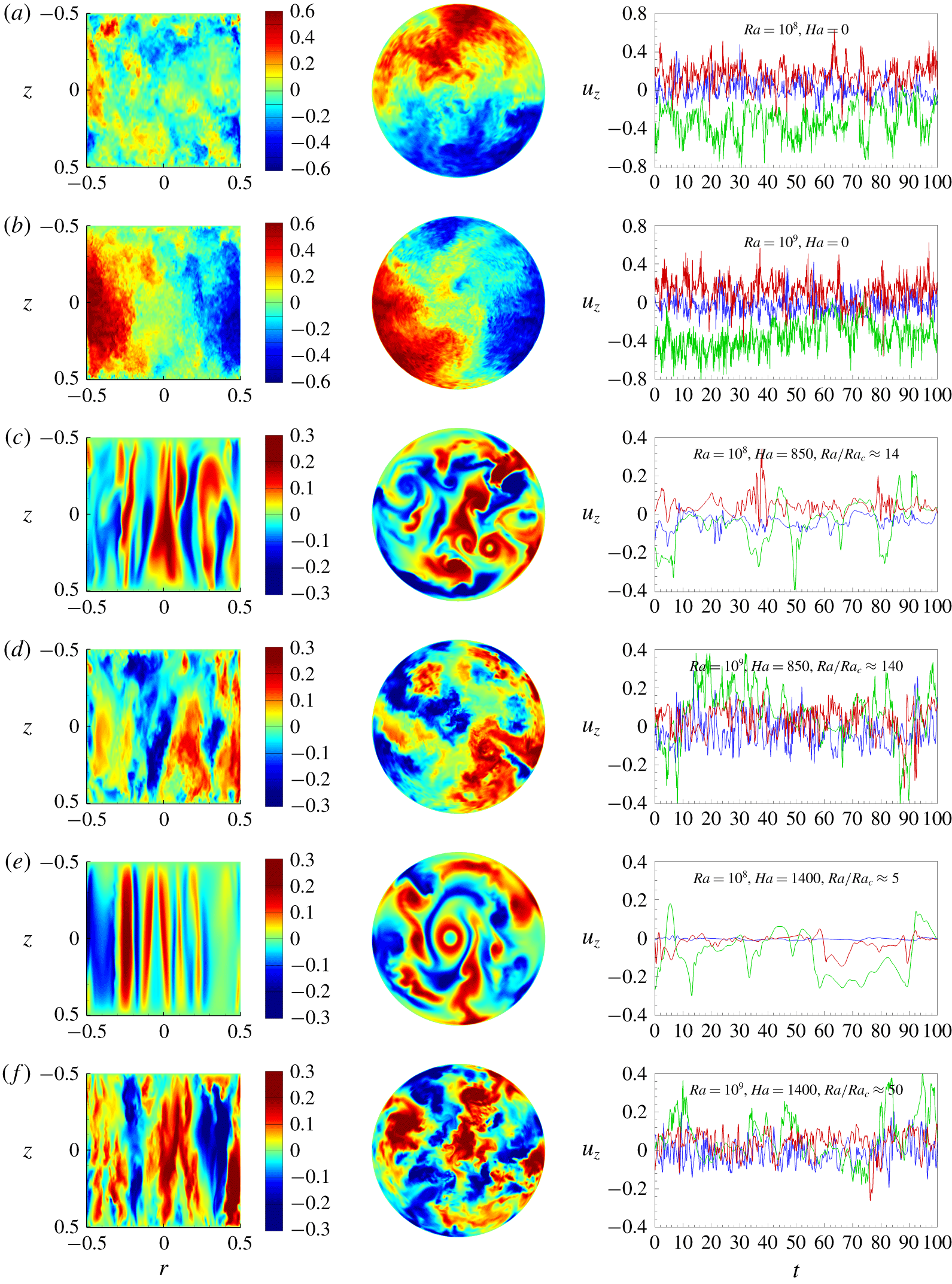
 $Re$ are less satisfactory, especially in flows with a strong magnetic field effect. The structure and character of the time evolution of the flow allow us attribute this, at least partially, to the effect of strong and slow (on the time scale of many tens of convective units – see e.g. figure 1e) fluctuations of velocity. Unfeasibly large averaging times are needed to eliminate this factor.
Snapshots of the vertical velocity in the vertical (left column) and horizontal mid-plane (centre column) cross-sections. Time signals of  $u_{z}$ (right column) at
 $\unicode[STIX]{x1D703}=0$,
 $z=0.25$ (—— red),
 $0$ (—— green) and
 $-0.25$ (—— blue), and
 $r=0.42$ (e),
 $0.44$ (a,c,d,f) and
 $0.46$ (b). The parameters
 $Ra$,
 $Ha$ and the ratio between
 $Ra$ and
 $Ra_{c}$ of the Chandrasekhar (Reference Chandrasekhar1961) stability limit are indicated in the right column.

3 Results
3.1 Spatial structure of the flow
The flow structure for several typical cases is illustrated in figure 1. Flows without a magnetic field (see figure 1a,b) are turbulent. The spatial structure in the horizontal cross-section (middle column) and the correlation between the velocity signals measured along a vertical line indicate the presence of a large-scale circulation (LSC) with upward or downward flow zones.
The magnetic field drastically changes the flow. We observe the suppression of small-scale velocity gradients and the formation of large-scale anisotropic structures dominating the flow (see the left and middle columns of figure 1c–f). This is associated with a reduction of amplitude and frequency of velocity fluctuations (see the right column of figure 1c–f) and, as we will discuss in § 3.2, an increase of  $Nu$ and
 $Re$. Similar flow transformations were detected in the recent measurements of Zürner et al. (Reference Zürner, Schindler, Vogt, Eckert and Schumacher2020) and in the simulations of Liu et al. (Reference Liu, Krasnov and Schumacher2018), Yan et al. (Reference Yan, Calkins, Maffei, Julien, Tobias and Marti2019) for lower Rayleigh numbers.
The strength of the magnetic field effect determining the degree of the flow transformation correlates with the ratio between  $Ra$ and
 $Ra_{c}$. At
 $Ra\gg Ra_{c}$ (see figure 1d,f), the large-scale velocity structures are anisotropic (elongated in the direction of the magnetic field) but susceptible to three-dimensional (3-D) instabilities and evolve on the background of 3-D small-scale velocity fluctuations. At
 $Ra$ larger, but not much larger than
 $Ra_{c}$ (see figure 1c,e), the anisotropy is much stronger and 3-D fluctuations are much weaker.
In the latter case, nearly Q2D upward and downward streams occupy the flow domain. Interestingly, these flows, in particular the flow at  $Ra/Ra_{c}\approx 5$ shown in figure 1(e), are principally different from the other recently identified Q2D magneto-convection regimes: the wall modes of Liu et al. (Reference Liu, Krasnov and Schumacher2018) and the cellular and columnar regimes found in an infinite horizontal layer by Yan et al. (Reference Yan, Calkins, Maffei, Julien, Tobias and Marti2019). The former is not surprising, since the simulations of Liu et al. (Reference Liu, Krasnov and Schumacher2018) find the wall-mode regimes at
 $Ra/Ra_{c}\sim 1$ or
 ${<}1$, but not at higher
 $Ra/Ra_{c}$. For example, the wall modes were not found at
 $Ra/Ra_{c}=4.05$.
The discrepancy with the results of Yan et al. (Reference Yan, Calkins, Maffei, Julien, Tobias and Marti2019) obtained for an infinite horizontal layer appears more significant. Unlike the ‘cells’ reminiscent of the linear instability modes or the ‘columns’ found in their simulations, the dominant feature of the flow in figure 1(e) can be described as a system of ascending and descending planar jets often originating at the sidewall and extending into the bulk of the flow. We should mention that the horizontal velocity is strong in this flow ( $\langle u_{r}^{2}+u_{\unicode[STIX]{x1D703}}^{2}\rangle _{V,t}/\langle u_{z}^{2}\rangle _{V,t}\approx 0.44$ in comparison to
 ${\approx}0.27$ for the case in figure 1f). The regime is reminiscent of Q2D extended vortex sheets often found in magnetohydrodynamic (MHD) turbulent flows with strong magnetic field effect (see e.g. Zikanov & Thess Reference Zikanov and Thess1998). The fact that this regime rather than the cellular or columnar regimes of Yan et al. (Reference Yan, Calkins, Maffei, Julien, Tobias and Marti2019) is realized in our flow can be attributed to smaller
 $Pr$ (
 $Pr=1$ was used by Yan et al. (Reference Yan, Calkins, Maffei, Julien, Tobias and Marti2019)) or, much more likely, the presence of sidewalls.
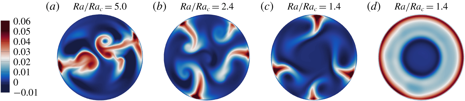
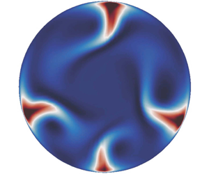
The wall-mode regime is found in our simulations at  $Ra/Ra_{c}\rightarrow 1$. As an illustration, figure 2 shows the instantaneous distributions of convective flux
 $u_{z}T$ in flows with
 $Ra=10^{7}$ (also used by Liu et al. (Reference Liu, Krasnov and Schumacher2018)) and several values of
 $Ha$. The structure of the wall modes is qualitatively similar to the structure observed by Liu et al. (Reference Liu, Krasnov and Schumacher2018) (see figure 2c). Significant flow and heat transfer are limited to tongue-like zones attached to the sidewall. There are noticeable differences, though. The entire wall-mode structure rotates clockwise or anticlockwise in our system. The effect of rotation is illustrated by the almost axisymmetric distribution of the time-averaged heat flux shown in figure 2(d). The travelling waves in the azimuthal direction were not observed in the linear stability analysis (Houchens et al. Reference Houchens, Witkowski and Walker2002). Another difference is the transformation of wall modes at increasing
 $Ra/Ra_{c}$. As in the simulations of Liu et al. (Reference Liu, Krasnov and Schumacher2018), the wall modes extend further from the wall. The new feature that can be plausibly attributed to rotation is that the wall-mode zones curve (see figure 2b) and form Q2D vortices (see figure 2a). We leave a detailed analysis of the properties and physical mechanisms of wall modes to future studies and only mention here that observed behaviour is qualitatively similar to that in RBC with rotation (Zhong et al. Reference Zhong, Ecke and Steinberg1991; Ecke et al. Reference Ecke, Zhong and Knobloch1992; Zhang et al. Reference Zhang, van Gils, Horn, Wedi, Zwirner, Ahlers, Ecke, Weiss, Bodenschatz and Shishkina2019).
Snapshots of the convective flux  $u_{z}T$ in the horizontal mid-plane of the cylinder at
 $Ra=10^{7}$ with:
 $Ra/Ra_{c}=5.0$,
 $Ha=450$ (a);
 $Ra/Ra_{c}=2.4$,
 $Ha=650$ (b); and
 $Ra/Ra_{c}=1.4$,
 $Ha=850$ (c). Time-averaged convective flux at
 $Ra=10^{7}$ and
 $Ha=850$ is shown in (d).

3.2 Global transport properties
All computed values of  $Nu$ and
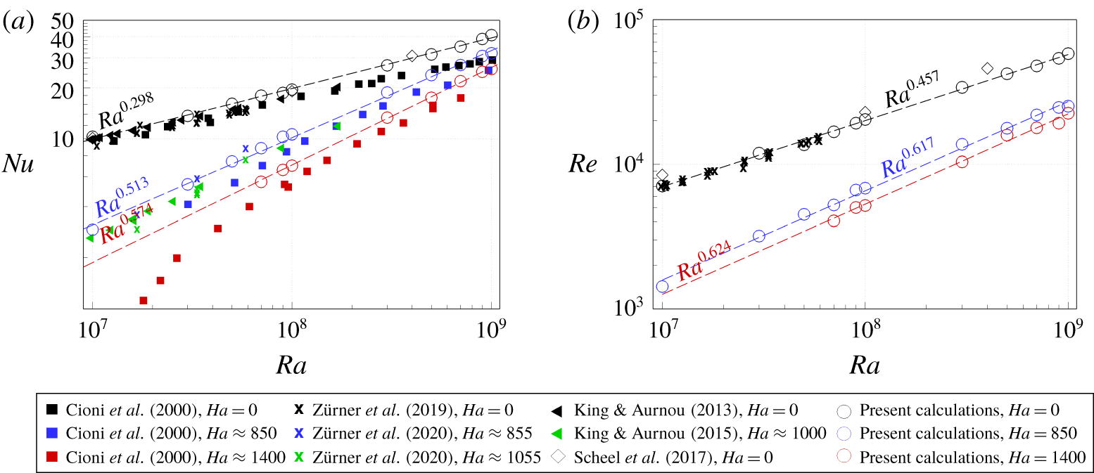
 $Re$ are listed in the supplementary material. They are also summarized and compared with the available experimental and numerical data in figure 3. The qualitative agreement between the numerical and experimental data is good. In particular, the increase of the slope of
 $Nu(Ra)$ and
 $Re(Ra)$ curves in flows with the magnetic field, which we discuss in detail below, is consistent between the simulations and the experiments. At the same time, the quantitative agreement is less convincing, with the computed values being consistently higher than in the experiments, especially in the experiment of Cioni et al. (Reference Cioni, Chaumat and Sommeria2000). This situation is typical for thermal convection in low-
 $Pr$ fluids and can be attributed to several known difficulties of the experimental procedure: (1) the ideal boundary conditions of constant temperature at the top and bottom plates cannot be accurately maintained; (2) the temperatures at the top and bottom boundaries are not measured directly, which usually leads to a slight overestimation of the Rayleigh number; (3) complete avoidance of heat losses through the sidewall is impossible; and (4) physical properties within a system are not constant, which results in inaccurate estimates of the Prandtl, Hartmann and Rayleigh numbers.
Nusselt number  $Nu$ versus
 $Ra$ (a) and Reynolds number
 $Re$ versus
 $Ra$ (b) with and without a magnetic field. Experimental and numerical data for
 $\unicode[STIX]{x1D6E4}=1$ are shown for comparison. Lines with slope
 ${\sim}Ra^{\unicode[STIX]{x1D6FD}}$ are plotted for guidance.

Estimates of the scaling behaviour of  $Nu$ and
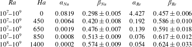
 $Re$ based on the data of our simulations are presented in table 1. Some of the respective lines are also shown in figure 3. The common regression method is applied to the computed time-averaged values to determine the exponents
 $\unicode[STIX]{x1D6FD}_{Nu}$ and
 $\unicode[STIX]{x1D6FD}_{Re}$ and their standard errors, and the constants
 $\unicode[STIX]{x1D6FC}_{Nu}$ and
 $\unicode[STIX]{x1D6FC}_{Re}$ in the approximations
 $Nu\approx \unicode[STIX]{x1D6FC}_{Nu}Ra^{\unicode[STIX]{x1D6FD}_{Nu}}$ and
 $Re\approx \unicode[STIX]{x1D6FC}_{Re}Ra^{\unicode[STIX]{x1D6FD}_{Re}}$.
For flows with  $Ha=0$, some disagreement with the data of Cioni et al. (Reference Cioni, Chaumat and Sommeria2000) is found (see figure 3a). At the same time, the computed value of
 $\unicode[STIX]{x1D6FD}_{Nu}$ is in good agreement with the value
 $0.29\pm 0.01$ for
 $Pr=0.025$ found in the experiments with the largest range
 $2\times 10^{5}\leqslant Ra\leqslant 8\times 10^{10}$ by Glazier et al. (Reference Glazier, Segawa, Naert and Sano1999) performed at
 $\unicode[STIX]{x1D6E4}=0.5,1,2$. The exponent
 $\unicode[STIX]{x1D6FD}_{Re}$ is consistent with
 $0.46\pm 0.02$ for
 $Pr=0.025$ and
 $0.42\pm 0.03$ for
 $Pr=0.029$ found in measurements by Takeshita et al. (Reference Takeshita, Segawa, Glazier and Sano1996) and Zürner et al. (Reference Zürner, Schindler, Vogt, Eckert and Schumacher2019), respectively, and with
 $0.45\pm 0.04$ for
 $Pr=0.021$ in numerical simulations by Scheel & Schumacher (Reference Scheel and Schumacher2017).
An imposed magnetic field reduces the rate of heat transfer and kinetic energy in the entire studied range of  $Ra$. At the same time, growth of
 $Nu$ and
 $Re$ becomes faster. In particular, the slope
 $\unicode[STIX]{x1D6FD}_{Nu}$ increases from
 $0.298$ at
 $Ha=0$ to approximately
 $0.574$ at
 $Ha=1400$. A similar increase is observed for
 $\unicode[STIX]{x1D6FD}_{Re}$ (see table 1 and figure 3). The results are consistent with the data of Cioni et al. (Reference Cioni, Chaumat and Sommeria2000), the only experiment in our range of interest of
 $Ra$ and
 $Ha$.
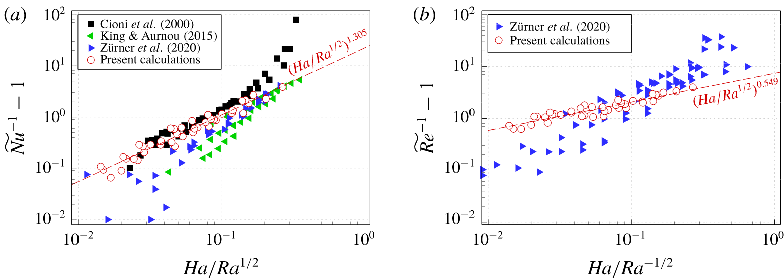
Normalized Nusselt number  $\widetilde{Nu}$ versus
 $Ha/Ra^{1/2}$ (a) and Reynolds number
 $\widetilde{Re}$ versus
 $Ha/Ra^{1/2}$ (b). Experimental data
 $\unicode[STIX]{x1D6E4}=1$ are shown for comparison. Lines with slope
 ${\sim}(Ha/Ra^{1/2})^{\unicode[STIX]{x1D6FD}}$ are plotted for guidance.

Scaling coefficients in the approximations  $Nu\approx \unicode[STIX]{x1D6FC}_{Nu}Ra^{\unicode[STIX]{x1D6FD}_{Nu}}$ and
 $Re\approx \unicode[STIX]{x1D6FC}_{Re}Ra^{\unicode[STIX]{x1D6FD}_{Re}}$ based on the data of the present simulations (see figure 3).

The Nusselt number  $\widetilde{Nu}=(Nu-1)/(Nu_{Ha=0}-1)$ and the Reynolds number
 $\widetilde{Re}=Re/Re_{Ha=0}$ normalized by their reference values at
 $Ha=0$ are shown in figure 4. The universal scaling behaviour of
 $\widetilde{Nu}=1/[1+\unicode[STIX]{x1D6FC}_{\widetilde{Nu}}(Ha/Ha_{c})^{\unicode[STIX]{x1D6FD}_{\widetilde{Nu}}}]$ and
 $\widetilde{Re}=1/[1+\unicode[STIX]{x1D6FC}_{\widetilde{Re}}(Ha/\sqrt{Ha_{c}})^{\unicode[STIX]{x1D6FD}_{\widetilde{Re}}}]$ was proposed by Zürner et al. (Reference Zürner, Schindler, Vogt, Eckert and Schumacher2020). To verify this hypothesis, we plot
 $1/\widetilde{Nu}-1$ and
 $1/\widetilde{Re}-1$ versus
 $Ha/Ra^{1/2}$ in logarithmic scales. The computed data provide
 $\unicode[STIX]{x1D6FD}_{\widetilde{Nu}}=1.305\pm 0.049$ and
 $\unicode[STIX]{x1D6FD}_{\widetilde{Re}}=0.549\pm 0.034$.
The qualitative agreement between the simulations and the experiments, especially with the experiments by Cioni et al. (Reference Cioni, Chaumat and Sommeria2000), is observed for  $\widetilde{Nu}$ at
 $Ra>Ra_{c}$ (
 $Ha/Ra^{1/2}\sim 0.1$) and
 $Ra\gg Ra_{c}$ (
 $Ha/Ra^{1/2}<0.1$) in figure 4(a). The results indicate that a universal power is approached for flows at high Rayleigh numbers. At the same time, the standard error is higher and the coefficient of determination (
 $R^{2}$) is lower than for the scaling
 $Nu\sim Ra^{\unicode[STIX]{x1D6FD}_{Nu}}$ presented above (
 $R^{2}=0.943$ in comparison to
 $R^{2}=0.998$ for
 $Nu\sim Ra^{\unicode[STIX]{x1D6FD}_{Nu}}$ at
 $Ha=1400$). A similar situation is observed for the normalized Reynolds numbers in figure 4(b).
We expect an increase of the exponents  $\unicode[STIX]{x1D6FD}_{\widetilde{Nu}}$ and
 $\unicode[STIX]{x1D6FD}_{\widetilde{Re}}$ in the wall-mode regime at
 $Ra\sim Ra_{c}$ (
 $Ha/Ra^{1/2}\sim 0.25$). However, the measurements of Zürner et al. (Reference Zürner, Schindler, Vogt, Eckert and Schumacher2020) for
 $1/\widetilde{Re}-1$ show a line with higher slope
 ${\sim}(Ha/Ha_{c})^{1.73\pm 0.05}$ for a wide range of
 $Ra$ and
 $Ha$. The discrepancy with this result and the presence of even stronger deviations in experimental data for moderate
 $Ra$ can be attributed to the limitations of the ultrasound Doppler velocimetry used to probe the flow field discussed by Zürner et al. (Reference Zürner, Schindler, Vogt, Eckert and Schumacher2020).
Estimates of the thickness of the thermal boundary layer are presented in the supplementary material. The common slope method used in the experiments (Takeshita et al. Reference Takeshita, Segawa, Glazier and Sano1996) and simulations (Liu et al. Reference Liu, Krasnov and Schumacher2018) is applied, i.e. the intersection point of the tangent of the time-averaged mean temperature profile near the sidewall and the horizontal line drawn through the mean value is taken. We only mention here that the results of the present simulations deviate by no more than  $2\,\%$ from the theoretical value
 $\unicode[STIX]{x1D6FF}_{T}\approx 1/(2Nu)$ of Grossmann & Lohse (Reference Grossmann and Lohse2001), even in the presence of a magnetic field.
4 Concluding remarks
We have performed DNS of RBC in a cylinder with imposed vertical magnetic field. The range of high  $Ra$ and
 $Ha$ never previously explored in numerical simulations was considered. The computations were performed on large grids with adequate resolution of internal features and boundary layers.
A new regime in the form of nearly Q2D upward and downward planar jets originating at the sidewalls and extending into the flow domain is identified at  $Ra$ larger, but not much larger, than
 $Ra_{c}$. The structures are reminiscent of Q2D extended vortex sheets found in MHD turbulence (see e.g. Zikanov & Thess Reference Zikanov and Thess1998). Our results also show the existence of rotating tongue-like wall modes at
 $Ra\rightarrow Ra_{c}$, in apparent qualitative similarity with rotating RBC (Ecke et al. Reference Ecke, Zhong and Knobloch1992; Zhang et al. Reference Zhang, van Gils, Horn, Wedi, Zwirner, Ahlers, Ecke, Weiss, Bodenschatz and Shishkina2019).
The results of our DNS are consistent with available experimental and numerical data. In particular, we find faster growth of  $Nu$ and
 $Re$ with
 $Ra$ in flows with strong magnetic fields. This effect can only be plausibly attributed to the formation of coherent large-scale Q2D structures in the flow field (see § 3.1). The scaling laws for normalized Nusselt and Reynolds numbers reveal the same tendency as the experimental data, namely that the global transport properties approach a universal power law at
 $Ra\gg Ra_{c}$.
The presented work is considered by the authors as the beginning of a larger and more detailed study. Future investigations of the system are undoubtedly warranted. In particular, it would be interesting to further analyse the properties and physical mechanisms of the newly discovered Q2D regime, the behaviour of wall modes, the transport properties at  $Ra>10^{9}$ and
 $Ha>1400$, and, finally, the apparent, albeit evidently incomplete, similarities between RBC with magnetic field and rotation.
Acknowledgements
Financial support was provided by the US NSF (Grant CBET 1803730) and the DFG grant KR 4445/2-1. Computer time was provided by the Computing Center of the Technische Universität Ilmenau and the Leibniz Rechenzentrum Garching within Large Scale project pr62se.
Declaration of interests
The authors report no conflict of interest.
Supplementary materials
Supplementary materials are available at https://doi.org/10.1017/jfm.2020.336.