


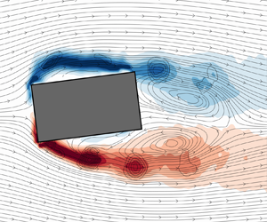



1. Introduction
One fundamental distinction between circular and rectangular cylinders lies in the presence of four well-defined separation points located at the edges of the rectangular cylinder, resulting in flat wall surfaces between the adjacent edges. Consequently, the wake flow becomes more intricate due to the presence of two predominant separation regions in the shear layer, namely the leading-edge (LE) separation and the trailing-edge (TE) separation (Saha, Biswas & Muralidhar Reference Saha, Biswas and Muralidhar2003; Inoue, Iwakami & Hatakeyama Reference Inoue, Iwakami and Hatakeyama2006; Prasanth & Mittal Reference Prasanth and Mittal2008; Singh & Biswas Reference Singh and Biswas2013; Shoukry & Mohany Reference Shoukry and Mohany2023). For elongated rectangular cylinders with an aspect ratio  $l/h > 3$, where the aspect ratio represents the ratio between the streamwise dimension
 $l$ and the cross-stream dimension
 $h$, both the leading and trailing edges shed vortices at high Reynolds numbers. The shedding from both edges exhibits synchronization to the same frequency, indicating the existence of a feedback loop between the pressure perturbations at the TE caused by vortex roll and formation, and the separation of the shear layer at the LE. Additionally, it is observed that the Strouhal number demonstrates a stepwise behaviour with respect to the aspect ratio (Okajima Reference Okajima1982; Nakamura & Nakashima Reference Nakamura and Nakashima1986; Ozono et al. Reference Ozono, Ohya, Nakamura and Nakayama1992; Mills et al. Reference Mills, Sheridan, Hourigan and Welsh1995; Tan, Thompson & Hourigan Reference Tan, Thompson and Hourigan1998).
In their pioneering work, Nakamura & Nakashima (Reference Nakamura and Nakashima1986) introduced the concept of leading-edge vortex shedding (LEVS) and termed the overall shedding mechanism as impinging-shear-layer instability. They proposed that this instability is independent of the mutual induction between the two shear layers originating from the lateral faces of the cylinder. To verify this hypothesis, a splitter plate was inserted into the wake of a rectangular cylinder with an aspect ratio of 5. Remarkably, the shedding frequency remained unchanged both before and after the insertion of the splitter plate. Similarly, Shaaban & Mohany (Reference Shaaban and Mohany2022) recently observed the same shedding mode during self-excited acoustic resonance, for a rectangular cylinder with an aspect ratio as low as 2. These findings underscore the presence of this shedding mode even at low aspect ratios and further highlight its nature as a resonant oscillation of the fluid.
Naudascher & Rockwell (Reference Naudascher and Rockwell1994) classified three distinct vortex shedding regimes for rectangular cylinders based on the aspect ratio. Type I, known as LEVS, is characterized by a separation bubble at the LE of the body. Type II is referred to as impinging leading-edge vortex (ILEV) instability and involves the shedding of LE vortices from the separation bubble at the LE, which subsequently interact with the TE vortices. Type III is the trailing-edge vortex shedding (TEVS), where vortices detach from the TEs of the rectangular cylinder. Hourigan, Thompson & Tan (Reference Hourigan, Thompson and Tan2001) later discovered a hybrid shedding mechanism that can occur at Reynolds numbers below 2000, representing a combination of the ILEV and TEVS regimes. They observed that the TE vortices are forced to modulate their frequency to align closely with the shedding frequency, enabling the shedding of LE vortices within one complete shedding cycle with proper phasing. This accommodation of the full shedding cycle wavelength along the length of the cylinder occurs due to the synchronization between the LE and TE shedding modes.
The stepwise behaviour in the Strouhal number is attributed to a locked-feedback mechanism between the frequency of the LE and TE vortices, with a wavelength that is directly correlated to the streamwise dimension of the cylinder. The mode progression is associated with the number  $n$ of vortices present on the lateral face of the rectangular cylinder between the leading and trailing edges. For rectangular cylinders with aspect ratios between 3 and 5, the first mode of the ILEV is characterized by one LE vortex on the lateral faces (i.e.
 $n = 1$). As the aspect ratio increases, the wavelength also increases until reaching a threshold that allows for the transition to the second ILEV mode (i.e.
 $n = 2$), which means two distinct vortex cores are formed along the lateral face.
Building upon the work of Nakamura & Nakashima (Reference Nakamura and Nakashima1986), the ILEVS mode is considered a resonant oscillation of the fluid that can be triggered when coupling with a resonant acoustic wave within an enclosure occurs. The feedback loop in this case is established through the pressure perturbation originating from the flow field discontinuity at the TE, which results from vortex production at the cylinder's TE. The formation of the LE vortices occurs due to the interaction of the shear layer with the LE. When the LE vortex passes the TE, a localized pressure pulse is generated due to strain concentration at a specific point. This pulse subsequently travels upstream, triggering the shedding of a LE vortex from the LE shear layer.
Parker & Llewelyn (Reference Parker and Llewelyn1972) revealed in their study that there could be four possible vortex shedding patterns depending on the cylinder's aspect ratio. (I) Cylinders with ( $l/h < 3.2$) experience flow separation at the LE with no reattachment to the cylinder's surface. The separated shear layer at the LE rolls into the wake, forming a regular vortex shedding street, which is also known as LEVS. (II) Cylinders with (
 $3.2 < l/h < 7.6$) exhibit a TE interaction with the LE vortices, producing the ILEV or TEVS mode. (III) Cylinders with (
 $7.6 < l/h < 16$) experience shear layer reattachment somewhere on the lateral face before the TE, forming a separation bubble that sheds vortices randomly. This shear layer behaviour results in irregular shedding patterns with no distinct vortex shedding street. (IV) Cylinders with (
 $l/h > 16$) experience a similar behaviour to those in (III), but the vortices shedding from the separation bubble dissipate before reaching the TE. Additionally, a regular shedding pattern exists under acoustic resonance conditions for high aspect ratios. Nakamura, Ohya & Tsuruta (Reference Nakamura, Ohya and Tsuruta1991) suggested that although for high aspect ratios (
 $l/h > 12$) there is no organized shedding pattern that can be detected, the shedding pattern observed by Stokes & Welsh (Reference Stokes and Welsh1986) is a manifestation of the ILEV inherited in the flow, with the acoustic field acting as an external forcing source to excite it. However, Mills, Sheridan & Hourigan (Reference Mills, Sheridan and Hourigan2003) proposed a contrasting hypothesis referred to as the TE shedding. They argued that the shedding pattern detected under resonant conditions in the study of Stokes & Welsh (Reference Stokes and Welsh1986) was not an instance of ILEV shedding as proposed by Nakamura et al. (Reference Nakamura, Ohya and Tsuruta1991) but rather a different shedding mechanism. Thus, one of the primary objectives of our research is to navigate through these conflicting viewpoints and clarify the effect of acoustic resonance on the unsteady flow structures around a rectangular cylinder. Such an endeavor will deliver a more unified understanding of the underlying shedding mechanisms at both resonant and non-resonant conditions.
For higher Reynolds numbers, two studies conducted by Okajima (Reference Okajima1982) and Igarashi (Reference Igarashi1984) have revealed that flow characteristics and aerodynamics remain relatively insensitive to the upstream Reynolds number beyond a value of approximately  $10^{4}$. However, the angle of incidence has a notable effect on shifting the separation points, thereby altering the free shear layer separation and resulting in wake rolling. This shift in separation points can ultimately impact the hydrodynamic loading, the Strouhal number of dominant shedding patterns and heat transfer coefficients. Furthermore, several studies have reported that changes in the shedding pattern in the wake can occur due to variations in shear layer separation dynamics caused by the angle of incidence (Zaki, Sen & Gad-El-Hak Reference Zaki, Sen and Gad-El-Hak1994; Sohankar, Norberg & Davidson Reference Sohankar, Norberg and Davidson1998). Knisely (Reference Knisely1990) thoroughly reviewed Strouhal number data from the literature for various aspect ratios and incidence angles. The general trend observed in most cases showed a rapid increase in the Strouhal number and a significant decrease in the aerodynamic forces at small angles of attack (
 $\alpha <15^{\circ }$). This trend is thought to be associated with the shear layer separation and subsequent reattachment to the cylinder's windward lateral face. The reattachment of the shear layer reduces pressure fluctuations in the wake, which, in turn, reduces the aerodynamic forces imposed on the rod. Other studies reported similar trends for Strouhal number and aerodynamic forces (Saha, Muralidhar & Biswas Reference Saha, Muralidhar and Biswas2000a; Dutta, Muralidhar & Panigrahi Reference Dutta, Muralidhar and Panigrahi2003; Sarioglu, Akansu & Yavuz Reference Sarioglu, Akansu and Yavuz2005).
Compared with the studies reporting on vortex shedding modes and aerodynamic forces, fewer investigations have focused on characterizing the velocity field and wake dynamics of rectangular cylinders. Work by Durão, Heitor & Pereira (Reference Durão, Heitor and Pereira1988), Lyn et al. (Reference Lyn, Einav, Rodi and Park1995), Lyn & Rodi (Reference Lyn and Rodi1994), Ozgoren (Reference Ozgoren2006), Hu, Zhou & Dalton (Reference Hu, Zhou and Dalton2006) and Kurtulus, Scarano & David (Reference Kurtulus, Scarano and David2007) employed various flow visualization techniques, such as particle image velocimetry (PIV) and laser Doppler velocimetry, to accurately construct the near and far wake velocity fields, time-averaged turbulence properties and phase-averaged streamline patterns. These approaches provide valuable insights into the wake flow topology, allowing for choosing the optimum configuration for different industrial applications and the development of effective techniques for suppressing vortex shedding. Igarashi (Reference Igarashi1984) implemented surface-oil flow and smoke to study the flow around a square cylinder at different angles of incidence. He divided the wake flow patterns into four different regimes based on the incidence angle, i.e. (I)  $0^{\circ }\leq \alpha \leq 5^{\circ }$: symmetric flow with perfect separation; (II)
 $5^{\circ }\leq \alpha \leq 13^{\circ }$: asymmetric flow with separation; (III)
 $14^{\circ }\leq \alpha \leq 35^{\circ }$: reattachment flow type; and (IV)
 $35^{\circ }\leq \alpha \leq 45^{\circ }$: wedge flow type. van Oudheusden et al. (Reference van Oudheusden, Scarano, van Hinsberg and Watt2005) reported the velocity field around a square cylinder using PIV at four different angles of incidence. For
 $\alpha = 0^{\circ }$, the boundary layer bifurcates into two branches from the midpoint on the square section in the cross-stream direction and then separates from the two leading sharp edges. The free shear layer rolls into the wake forming two distinct recirculation regions, a primary region that is due to the large-scale vortex formation in the wake and a secondary region at the cylinder's lateral faces in the streamwise direction. Between
 $\alpha = 5^{\circ }$ and
 $\alpha = 10^{\circ }$ the two recirculation regions merged together into one region in the wake. Flow reattachment was observed between
 $\alpha = 10^{\circ }$ and
 $\alpha = 15^{\circ }$. The topological analysis of this study did not precisely match the flow topology equation outlined by Hunt et al. (Reference Hunt, Abell, Peterka and Woo1978) due to the difficulties in capturing the near-surface flow topology because of the laser reflections and insufficient spatial resolution or image count in the PIV window size. To compensate for the flow visualization challenges, multiple investigators have conducted computational fluid dynamics studies on square cylinders to capture the near-surface, wake topology and unsteady flow characteristics (Taylor & Vezza Reference Taylor and Vezza1999; Saha, Muralidhar & Biswas Reference Saha, Muralidhar and Biswas2000b; Cheng, Whyte & Lou Reference Cheng, Whyte and Lou2007).
In light of the previous discussion, for square and rectangular cylinders, the shear layer behaviour and the periodic flow structures in the wake are found to be sensitive to the aspect ratio and angle of incidence. However, most of the studies focused on high aspect ratios ( $3 < l/h <16$) as it is assumed that below this range the shear layer is said to be stable with a natural shedding process occurring in the wake. This study aims to address this gap by employing PIV techniques in a high-speed wind tunnel to investigate the flow dynamics around a rectangular cylinder with an aspect ratio of 2 at various angles of incidence. The investigation will be conducted both with and without self-excitation of acoustic perturbations. The primary objective is to determine whether the resonant mode previously reported by Stokes & Welsh (Reference Stokes and Welsh1986) arises from a coupling with the inherent ‘ILEV’ instability, as suggested by Nakamura et al. (Reference Nakamura, Ohya and Tsuruta1991) or if it represents a distinct vortex shedding mechanism, as proposed by Mills et al. (Reference Mills, Sheridan and Hourigan2003). By examining these aspects, we seek to gain a comprehensive understanding of the flow dynamics and the mechanisms involved in vortex impingement from different edges of the rectangular cylinder. Furthermore, this study will shed light on the modulation occurring between the LE and TE vortices. Acoustic resonance, being a global feedback mechanism, plays a crucial role in modulating the overall system frequency. The detailed analysis and observations from this study will contribute to a better understanding of the complex flow behaviour and the impact of acoustic resonance on the flow patterns around rectangular cylinders.
2. Experimental set-up
In this section we delineate the experimental apparatus and configurations employed for various measurements, encompassing both pressure measurements and flow visualization techniques.
2.1. Wind tunnel facility
Experiments were conducted in an open-loop wind tunnel that has a test section measuring 762 mm in length, 254 mm in height and 127 mm in width. This test section is made out of acrylic to allow for flow visualization.
To ensure uniform flow distribution in the spanwise direction, pressure measurements were conducted at 11 different locations along the cylinder's span, covering a wide range of Reynolds numbers. The results indicated minimal spanwise variation in the mean base pressure coefficient, falling within the experimental uncertainty of the measurements. All tested cases were positioned at a distance of 381 mm from the parabolic bell mouth entrance. At this location, hot-wire measurements were conducted, revealing that the transverse flow uniformity deviated by a maximum of 1 % from the free stream velocity. Analysis of the fast Fourier transform (FFT) of the natural turbulence spectrum revealed no observable peaks within the frequency range of interest. Throughout the velocity range, the maximum turbulence intensity was carefully measured and found to be below 0.8 %. The experiments were conducted under controlled environmental conditions, maintaining a temperature of  $25\,^{\circ }{\rm C}$ and 50 % humidity. Indoor climate monitoring was performed using an indoor climate sensor to ensure consistent conditions throughout the experiments. An optical-grade clear acrylic rectangular cylinder was employed, with a starting position of zero angle of incidence and dimensions of
 $h= 1.27$ cm in the cross-stream direction and
 $l = 2.54$ cm in the streamwise direction (see figure 3). To achieve precise control of the incidence angle, a laser-cut acrylic window with a dial mechanism was utilized. The dial allows for rotation and locking at specific orientations via a countersunk screw and nut externally mounted to the wind tunnel.
2.2. Acoustic pressure measurements
The acoustic pressure signal was recorded for 120 s during each measurement across the entire velocity range, spanning speeds from  $20\,{\rm m}\,{\rm s}^{-1}$ to
 $150\,{\rm m}\,{\rm s}^{-1}$, with incremental steps of
 $2.76\,{\rm m}\,{\rm s}^{-1}$. The velocity range corresponded to a Reynolds number, based on the streamwise length of the rectangular cylinder, ranging from
 $Re_{l} = 3.5 \times 10^{4}$ to
 $2.5 \times 10^{5}$, when the cylinder's angle of incidence was zero. This was achieved by using a flush-mounted pressure microphone strategically positioned on the top wall of the test section, directly above the centre of the cylinder. This position corresponded to the maximum pressure amplitude of the transverse acoustic mode, which was determined in a separate experiment using an array of flush-mounted microphones on the top wall at different streamwise positions. Details of this experiment are omitted here for brevity. A sampling frequency of 20 kHz was employed that was far above the targeted shedding frequencies. Welch's modified periodogram method, with a 50 % overlap and a resolution of 1 Hz, was applied to analyse the pressure signal and generate the frequency spectrum using FFT. To isolate and accurately capture the desired pressure values, a band-pass filter with a range of
 ${\pm }50$ Hz centred around the dominant frequency peak was employed. This filtering process enabled the extraction of relevant pressure information. Subsequently, the resulting filtered pressure signal was used to calculate the root-mean-square (r.m.s.) value of the pressure (
 $P_{rms}$), which was then normalized and presented as
 $P^{*}$ using the equation
 \begin{equation} P^{*}=\frac{2P_{rms}c}{\rho U_{\infty}^3}, \end{equation}
where  $c$ is the speed of sound (
 ${\rm m}\,{\rm s}^{-1}$),
 $\rho$ is the air density (
 ${\rm kg}\,{\rm m}^{-3})$ and
 $U_{\infty }$ is the mean flow speed (
 ${\rm m}\,{\rm s}^{-1}$). The cubic dependence of the acoustic pressure with the flow velocity was first reported by Keefe (Reference Keefe1962) and later confirmed by Mohany & Ziada (Reference Mohany and Ziada2005).
As the shedding patterns evolved in the cross-stream direction, they induced acoustic pressure perturbations in the transverse direction. Consequently, excitation of odd-numbered transverse acoustic modes occurred, facilitated by the cylinder's precise positioning at the centre of the duct height (i.e. acoustic particle velocity antinodes of the  $\lambda /2$,
 $3\lambda /2$ and
 $5\lambda /2$ modes), as shown in figure 1, which illustrates the pressure distribution of the first three odd-numbered acoustic modes in the transverse direction. The theoretical values of these modes can be calculated using the equations
 \begin{equation} f_{a(1)}=\frac{c}{2H},\quad f_{a(3)}=\frac{3c}{2H},\quad f_{a(5)}=\frac{5c}{2H}, \end{equation}
where  $H=254$ mm is the height of the test section.
Schematic representation of the acoustic pressure distribution inside the duct for the first three odd-numbered transverse modes.

When the frequency of the vorticity shedding coincides with the natural frequency of an acoustic duct mode, resonance may occur if the flow excitation energy is higher than the acoustic damping of the system. This resonance establishes a feedback loop between the flow and the sound field, leading to the amplification of acoustic energy and the generation of acute noise. The interaction between the flow dynamics and the acoustic field significantly influences the wake topology (Blevins Reference Blevins1984; Mohany & Ziada Reference Mohany and Ziada2009; Islam, Shaaban & Mohany Reference Islam, Shaaban and Mohany2020).
2.3. Particle image velocimetry
In this study the LaVision system was utilized to capture and analyse the instantaneous velocities of the flow field within the two-dimensional laser sheet domain. Figure 2 illustrates the complete PIV set-up. The utilization of the PIV system ensured accurate and comprehensive velocity measurements, enabling a detailed examination of the flow dynamics with and without acoustic perturbations.
Schematic of the complete PIV set-up, which includes a Nd-YAG laser light source, optical lens and mirrors, a CCD camera, a timing box and a seeding device. The PIV set-up is time synchronized to the pressure microphone at the wall of the test section. The signal from the microphone was also transmitted to an oscilloscope for monitoring purposes.

2.3.1. Flow field seeding and illumination
In this study, atomized di-ethyl-hexyl-sebacate with an average particle size of  $1\,\mathrm {\mu }{\rm m}$ was used for flow seeding. The measurement plane was illuminated by a double-head 532 nm Nd:YAG pulsed laser operating in a double pulse mode with a peak power output of 200 mJ. A precise linear actuation mechanism was employed to position the laser sheet in the middle of the
 $x$–
 $y$ plane. The laser sheet illuminated the test section from the bottom, passing through an optical-grade acrylic wall. The time between pulses was adjusted to ensure capturing the maximum particle displacement within a quarter of the interrogation window used for vector calculation. Image pairs from two successive frames were processed, with specific regions such as the cylinder area and any surface reflections masked out to ensure accurate analysis.
2.3.2. Image capturing and acquisition
To capture the flow images, a 12-bit charged-coupled device (CCD) camera operating in a double frame mode was utilized. The camera had a maximum resolution of  $2752\times 2200$ pixels. In order to enhance the image acquisition process, a green light filter matching the wavelength of the laser was installed on the camera. The camera was directly connected to a personal computer, enabling real-time image transfer and analysis. The camera shutter was synchronized with the laser pulsing to ensure precise timing for capturing the flow field. This synchronization was achieved through the DaVis software, which facilitated the coordination between the camera and the laser. To improve the accuracy of the flow measurements, dynamic filters were applied during the data processing stage. These filters were designed to eliminate background noise and remove any false vectors from the analysed flow field.
To conduct measurements during off-resonance conditions, a series of images were captured, representing various shedding cycles. To reconstruct a consistent shedding cycle, proper orthogonal decomposition (POD) analysis was employed using a dataset comprising 1200 images. This facilitated the identification and extraction of the dominant flow structures and shedding patterns.
Phase-locked PIV measurements were conducted during self-excited acoustic resonance to synchronize with the shedding mode. This synchronization was achieved by utilizing the acoustic pressure cycle as a reference signal. The signal was captured by a flush-mounted microphone in real time and displayed on an oscilloscope for visualization. A timing unit then synchronized the frequencies of the camera and the laser with the acoustic pressure cycle frequency. By dividing the acoustic pressure cycle into eight phases, the camera captured pairs of images at consistent intervals. Specifically, 250 instantaneous pairs of images were captured, with each pair corresponding to a phase interval of  $45^{\circ }$ on the acoustic pressure cycle. This approach ensured that PIV measurements were performed at precise and consistent phases in the flow/acoustic cycle.
2.3.3. Imaging and post processing
The image acquisition and post-processing were carried out using DaVis 10.0 software. To extract accurate velocity information, the interrogation window technique was applied in two steps. In the first step, a single pass was performed with an initial interrogation window size of  $64\times 64$ pixels and a 50 % overlap. This step helped capture the overall flow features and provided an initial estimation of the velocity field. For the second step, four passes were performed using a smaller interrogation window size of
 $24\times 24$ pixels with a 50 % overlap. This finer resolution allowed for a more detailed analysis of the flow field and improved the accuracy of velocity measurements. To ensure high-quality results, post-processing techniques were employed. Faulty vectors were identified and removed, and denoising filters were applied to obtain a smooth flow field. In regions where illuminated particles were missing, dynamic interpolation techniques were utilized to estimate particle displacements based on the surrounding particles’ motion. Spatial sliding filters were also applied to further enhance the quality of the flow field. Depending on the specific requirements of each case, different sliding filters such as Gaussian, minimum and maximum filters were utilized to optimize the results. These filters helped in reducing noise and refining the spatial distribution of the velocity field.
3. Flow under non-resonant condition
In this section we examine the flow dynamics around the cylinder with varying angles of incidence, ranging from  $0^{\circ }$ to
 $90^{\circ }$, in conditions devoid of acoustic coupling. The coupling between the flow structures and the transverse acoustic modes of the duct (acoustic resonance) is studied in § 4. In § 3.1 the variation of the Strouhal number with respect to the incidence angle is presented and cross-validated against prior research. Subsequently, § 3.3 delves into the spatio-temporal progression of the vorticity field in the vicinity of the cylinder. To do this, we construct phase-averaged flow fields based on the temporal coefficients of the two dominant POD modes introduced in § 3.2.
3.1. Strouhal number of natural vortex shedding
Figure 3 shows the Strouhal number  $St_{h'}$, based on the projected cross-stream dimension
 $h'$, corresponding to the natural vortex shedding periodicity from a rectangular cylinder at different flow incidence angles. The utilization of
 $h'$ is solely for the purpose of comparing with the results of Knisely (Reference Knisely1990). However, since the formation of vortices dictates the Strouhal number, normalizing it by the projected length in the streamwise direction
 $l'$ is more appropriate, as outlined in § 4. The Strouhal number shown in figure 3, derived from the FFT analysis of the acoustic pressure signal, accurately mirrors the dominant shedding mode. Initially, the Strouhal number stands at a value of 0.09 for zero angle of incidence. As the cylinder begins to tilt, the Strouhal number sharply ascends to around 0.18, indicating substantial alterations in the wake flow characteristics, which are discussed in detail in this section. At an incidence angle of approximately
 $\alpha \approx 60^{\circ }$, the Strouhal number trend shows an inflection point and begins to descend, reaching a value of about 0.15 at
 $\alpha = 90^{\circ }$. This observation underscores a significant transformation in the flow topology beyond the symmetric wedge angle, which is around
 $\sim 63^{\circ }$ for the case presented in this paper with an aspect ratio of 2. This angle represents the symmetric configuration for the rectangular cylinder in both cross-stream and streamwise directions. The Strouhal number obtained in this study for all the investigated flow incidence angles aligns well with existing literature, reflecting both the values and the trend associated with changes in the angle of incidence.
Strouhal number  $St_{h'}$ of natural shedding measured under non-resonant conditions at different angles of incidence
 $\alpha$. Open black circles: Knisely's experimental measurements at
 $Re=4.4\times 10^4$; open red squares: present study at
 $Re=4.6\times 10^4$.

3.2. Leading POD modes
In § 3.3 we explore the shedding topology through the construction of a phase-averaged flow field. The overarching objective here is threefold: (i) to quantify the energy associated with each mode, (ii) to chronicle the temporal evolution of the wake flow structures and (iii) to map out the spatial characteristics of the flow. To fulfil this objective, the POD modes are extracted denoted by  $\psi _{k}(x)$, eigenvalues (
 $\lambda _{k}$) and temporal coefficients (
 $a_{k}$). The mode number (
 $k$) represents each mode's contribution to the turbulent kinetic energy (TKE) within the wake (van Oudheusden et al. Reference van Oudheusden, Scarano, van Hinsberg and Watt2005; Perrin et al. Reference Perrin, Braza, Cid, Cazin, Barthet, Sevrain, Mockett and Thiele2007). In the context of bluff body wakes, the dominant pair of POD modes encapsulates the majority of the inherent TKE resulting from the high vorticity content of the large-scale vortices shed in the wake.
As depicted in figure 4(a), the principal pair of modes accounts for a range of 38–56 % of the total TKE. Notably, for the incidence angles  $\alpha = 0^{\circ }$ and
 $\alpha = 5^{\circ }$, the total energy within the first pair is significantly lower compared with the other angles of incidence. Specifically,
 $\alpha = 5^{\circ }$ demonstrates the least energy encapsulated within the first pair of modes. As the incidence angle increases, there is a corresponding increase in the energy contained within the first pair of modes. This implies that the shedding process at the initial two incidence angles might be subject to perturbations from turbulence, flow reattachment or flow instabilities. However, beyond these angles, the shedding pattern exhibits enhanced coherence, with reduced random turbulence and fewer formations of small-scale vortical structures.
Proper orthogonal decomposition on the PIV data for the angle of incidence  $\alpha =0$: (a) energy distribution of the POD modes in the TKE (
 $\lambda _{k}$), and (b) scatter plot of the temporal coefficients
 $a_{1}$ and
 $a_{2}$. The definition of the red circle is given by (3.1).

The POD method is employed to acquire phase-averaged data. Fortunately, the majority of the TKE is concentrated within the first pair of POD modes, as depicted in figure 4(a). In figure 4(b) a scatter plot of the temporal coefficients ( $a_{1}$ and
 $a_{2}$) derived from the snapshot POD post-analysis data for the incidence angle
 $\alpha = 0^{\circ }$ is presented. The data scatter forms an ellipse, conforming to the equation
 \begin{equation} \frac{\overline{a_1(\phi)}^2}{2 \lambda_1}+\frac{\overline{a_2(\phi)}^2}{2 \lambda_2}=1, \end{equation}
where  $\overline {a_j(\phi )}$ represents the mean value of the temporal coefficient
 $a_j$ at phase
 $\phi$, indicated by a red circle in figure 4(b). The terms
 $\lambda _1$ and
 $\lambda _2$ correspond to the eigenvalues of the dominant pair of POD modes. To determine the phases of the instantaneous flow field, the following equation is utilized:
 \begin{equation} \phi(t)=\tan ^{{-}1}\left[\frac{\sqrt{\lambda_2} a_1(t)}{\sqrt{\lambda_1} a_2(t)}\right]. \end{equation}
The entirety of the instantaneous flow field data is categorized into several bins, with the quantity determined by (3.2). To capture the evolution of the shear layer and its subsequent roll into the wake, the instantaneous flow fields are divided into 16 bins. Consequently, there is a phase difference of  $22.5^{\circ }$ between every pair of successive phases.
3.3. Phase-averaged flow topology
3.3.1. Cases with incidence angles  $\alpha =0$ and $5^\circ$


Presented in figure 5 is the phase-averaged vorticity field with the streamlines superimposed, which is constructed by averaging the fields in the  $\phi$ angular sector defined by (3.2). There exists a phase difference of
 $180^{\circ }$ between the columns on the left and right, this exact phase shift is chosen for its vivid illustration of the alternation in the shear layer and flapping behaviour. A hyperbolic stagnation point, denoted by a red dot, is introduced to the diagram. This point, representing a saddle in the streamfunction
 $\nabla ^2 \psi =-\omega _z$, can be visually identified from the distribution of the wake streamlines. Due to its inherent instability and the resulting flow divergence, the hyperbolic stagnation point serves as a valuable indicator for identifying the instant of large-scale vortex separation from the shear layer. For figure 5(a,b) (
 $\alpha =0$), the flow separates from the LEs (windward edges) without evidence of flow reattachment or impingement on the lateral faces of the cylinder. The shear layer rolls into the wake, forming large-scale vortices through mutual induction between the flapping shear layers, which exhibit a pure LEVS mode. Moving to
 $\alpha = 5^{\circ }$, the shear layer separates from the windward upper edge mainly rolling into the wake, but there is partial shear layer reattachment to the windward lateral face, evident from the shear layer evolution from the LE and streamlines paths. However, the shear layer separated from the windward lower edge shows no interaction with the cylinder, and the vortex detaches further downstream.
Phase-averaged vorticity field constructed employing the first pair of POD modes. Positive vorticity in red, negative in blue, with the streamlines superimposed at  $U_{\infty }= 19.32\,{\rm m}\,{\rm s}^{-1}$ for all the tested angles of incidence
 $\alpha$ from 0 and
 $90^\circ$ (here up to 30). Two phases of the mean oscillating cycle,
 $\phi =0$ (a,c,e,g,i) and
 $\phi =180^\circ$ (b,d, f,h,j), are shown for each angle of incidence. (Continued in figure 6.)

Phase-averaged vorticity field constructed employing the first pair of POD modes. Positive vorticity in red, negative in blue, with the streamlines superimposed at  $U_{\infty }= 19.32\,{\rm m}\,{\rm s}^{-1}$ for all the tested angles of incidence
 $\alpha$ from 0 and
 $90^\circ$ (here
 $75^\circ$ and
 $90^\circ$). Two phases of the mean oscillating cycle,
 $\phi =0$ (a,c) and
 $\phi =180^\circ$ (b,d), are shown for each angle of incidence.

3.3.2. Cases with incidence angles $\alpha \geq 10$

Starting from  $\alpha = 10^{\circ }$ up to
 $\alpha = 30^{\circ }$, the upper shear layer remains fully attached to the windward lateral face, while vortices shed from the TE. Meanwhile, the lower shear layer separates from the windward lower edge and sheds into the wake. It is evident that the leeward lower edge contributes to shaping the lower shear layer vortex. The shedding pattern can be identified as a hybrid LEVS/TEVS mode for these cases. The consistency of the shedding mode and shear layer behaviour across these cases can be attributed to the angle of incidence range. This range lies above the threshold of flow reattachment, approximately
 $5^{\circ }$ (Knisely Reference Knisely1990), but remains below the symmetric wedge angle of incidence. Moving to figure 6, at
 $\alpha = 75^{\circ }$, the lower shear layer separates from the windward upper edge and impinges on the TE, while the upper shear layer separates at the leeward upper edge with no evidence of flow reattachment. The vortex cores are significantly larger compared with the previous cases, attributed to the fact that this angle of incidence exceeds the symmetric wedge angle. Beyond this angle, the lower shear layer reattaches to the windward face near the TE, and the windward lateral face acts as an impinging surface rather than having the flow fully attached to it. Therefore, the shedding mode can be designated as the LEVS/ILEVS mode from the upper and lower shear layers, respectively. At an angle of incidence of
 $\alpha = 90^{\circ }$, a spatio-temporal symmetry manifests due to the inherent symmetry of the cylinder, resulting in a LEVS mode, similar to the case at
 $\alpha = 0^{\circ }$. However, the vortex cores appear notably larger and less elliptical in shape. This occurrence can be attributed to two primary reasons. Firstly, a reduced streamwise dimension amplifies the momentum of the shear layer as it rolls into the wake, fostering the formation of a vortex with enhanced vorticity content. Secondly, the expanded cross-stream dimension allows for a more substantial gap between the separation edge and the wake centreline, providing a wider spatial range for the vortex to form.
4. Flow-sound interaction response
This section focuses on the flow–acoustic coupled response of the rectangular cylinder at various angles of incidence. The objective is to understand how the different shedding modes are selected in response to transverse acoustic perturbations.
4.1. Overall picture
Figure 7 depicts the power spectral density (PSD) of the acoustic pressure measured at four distinct flow velocities: two prior to the onset of acoustic resonance excitation and two during its occurrence. Before acoustic resonance excitation, a dominant shedding mode corresponding to  $St = 0.18$ is evident in the spectrum, with its amplitude increasing with the flow velocity. Notably, the third acoustic mode is strongly excited instead of the expected first mode, reaching an amplitude exceeding
 $1200\,{\rm Pa}\,{\rm Hz}^{-1}$. This sudden coupling with the third acoustic mode appears to be triggered by vorticity shedding that is undetectable during the off-resonance conditions. The absence of excitation of the first acoustic mode by the natural vortex shedding is attributed to the third acoustic mode being triggered at a lower flow velocity than the coincidence between the natural shedding at
 $St = 0.18$ and the first acoustic mode at approximately 675 Hz. The amplitude of the acoustic pressure during the excitation of the third mode is remarkably high, and the flow structures corresponding to a Strouhal number of 0.6 are in a locked-in state, as we shall see in § 4.2, preventing the manifestation of acoustic resonance between the first acoustic mode and the natural shedding at
 $St = 0.18$. A similar phenomenon of sudden mode coupling, not aligning with the observed Strouhal progression, akin to what is observed in our study, was noted by Welsh & Gibson (Reference Welsh and Gibson1979), where sudden resonance excitation occurred. They observed substantial differences in the flow visualization using a traditional smoke method before and during this abrupt acoustic resonance, identifying it as contingent upon rod geometry, an observation later supported by Nakamura et al. (Reference Nakamura, Ohya and Tsuruta1991) for larger aspect ratios ranging from 3 to 16, primarily emphasizing the effect of the aspect ratio on the flow structure. This finding underscores the fact that acoustic resonance excitation can augment the streamwise length of the cylinder, thereby facilitating the emergence and sustenance of the ILEV/TEVS shedding pattern. This is further validated using the phase-locked PIV measurements presented in figure 9.
The PSD (i) before ( $U=26\,{\rm m}\,{\rm s}^{-1}$), (ii) just before (
 $U=55\,{\rm m}\,{\rm s}^{-1}$), (iii) after (
 $U=76\,{\rm m}\,{\rm s}^{-1}$) and (iv) at the peak (
 $U=110\,{\rm m}\,{\rm s}^{-1}$) of acoustic resonance, for
 $\alpha =0$. The PSD of the acoustic pressure increases from about
 $2\,{\rm Pa}\,{\rm Hz}^{-1}$ for vortex shedding at
 $St=0.18$ without resonance, to about
 $1200\,{\rm Pa}\,{\rm Hz}^{-1}$ by resonating with the third acoustic duct mode at
 $St=0.6$.

Figure 8 represents the amplitude and the frequency of the dominant flow instabilities from the cylinder, as extracted from the pressure spectra (refer to figure 7 for an example), for a range of upstream flow velocities and how they couple with different transverse acoustic modes. The normalized acoustic pressure is plotted on the  $y$ axis, while the secondary
 $y$ axis represents the peak frequency detected in the pressure spectra. The green shade resembles the region where self-excited acoustic resonance is observed.
Aeroacoustic response of the rectangular cylinder at different angles of incidence  $\alpha$ for increasing flow velocity
 $U$. The green shade resembles the region where self-excited acoustic resonance is observed. The data points (i,ii,iii and iv) shown in (a) are taken from figure 7. (Dashed Strouhal line: from literature; solid Strouhal line: measured.)

4.2. Case $\alpha =0$

Figure 8(a) illustrates the shedding progression from the rectangular cylinder at zero angle of incidence. The shedding frequency gradually increases in a consistent manner up to a flow velocity of  $U{_\infty }=73.41\,{\rm m}\,{\rm s}^{-1}$ where a sudden frequency jump occurs accompanied by a rapid increase in the normalized acoustic pressure and both frequencies are locked-in. The shedding frequency experiences a significant jump, increasing approximately fourfold from
 $f_{s} = 469$ Hz to
 $f_{s} = 1931$ Hz, which is close to the frequency of the third acoustic transverse mode of the duct. This clear frequency lock-in suggests the occurrence of self-excited acoustic resonance. As mentioned earlier, Welsh & Gibson (Reference Welsh and Gibson1979) observed a similar phenomenon with a rectangular cylinder possessing an aspect ratio of 5. Intriguingly, they reported a sudden stimulation of the duct's primary transverse mode, with the frequency abruptly doubling. This event was ascribed to what they termed ‘excited vortex shedding.’ Nevertheless, a definitive source of this excitation was not substantiated, as their study lacked the implementation of modern flow visualization techniques. Nakamura et al. (Reference Nakamura, Ohya and Tsuruta1991) later stated that this is attributed to the ‘ILEV’ being excited. They stated two main reasons for this hypothesis: first, this is an intrinsic masked characteristic of coherent flow structures in turbulent flows (Taneda Reference Taneda1983) that can be excited by an externally tuned source; second, the frequency at which the jump took place matches the natural ILEVS frequency. The Strouhal number that matches the jump in our case is
 $St_{l'}= 0.6$ (shown as a dotted line in figure 8a), which is exactly equal to the first mode of the ILEV for elongated rectangular rods with an aspect ratio ranging from 3 to 5 as reported in the literature, (see, for example, Okajima Reference Okajima1982; Nakamura & Nakashima Reference Nakamura and Nakashima1986; Ozono et al. Reference Ozono, Ohya, Nakamura and Nakayama1992; Mills et al. Reference Mills, Sheridan, Hourigan and Welsh1995). To resolve whether this constitutes an inherent ILEV or it is reflective of a natural vortex shedding mode, flow–acoustic phase-locked PIV measurements are conducted and will be discussed in § 5.
4.3. Case $\alpha =5^\circ$

Looking at figure 8(b), which shows the aeroacoustic response at  $\alpha = 5^{\circ }$, one can notice that there are only data points during resonance excitation and no data points outside acoustic resonance excitation. This is because outside of acoustic resonance, no distinct peaks are observed in the spectra of the acoustic pressure signals. Rockwell (Reference Rockwell1977) reported that there are no distinct peaks in the velocity fluctuations spectrum for a square cylinder at an angle of incidence
 $\alpha = 14^{\circ }$, which means that there is no detectable contribution to the vortex shedding process. However, for higher
 $\alpha$ values, the distinct peaks reappear again, which was attributed to the flow reattachment. Since the rectangular cylinder employed in our study has
 $l/h= 2$, this phenomenon occurs at a substantially lower
 $\alpha$. Even though this case shows no dominant peaks in the acoustic pressure spectra, the POD analysis shown in figure 4 can identify organized turbulent fluctuations that form this shedding mode. However, the flow reattachment destabilizes the mode and that is why this case showed the least turbulent energy in the first two modes. Additionally, as can be seen in figure 8(b), multiple acoustic modes are excited and they are coinciding with two main Strouhal lines, corresponding to
 $St_{l'}= 0.6$ and
 $St_{l'}= 1.21$, respectively. It is intriguing to observe that the transitions between the different shedding modes occur instantaneously without any lock-out periods. The switch between the first and the third modes, as well as the fifth and the third modes, happens abruptly. During acoustic resonance excitation, the vortices exhibit spanwise correlation (Islam et al. Reference Islam, Shaaban and Mohany2020), and the vortex shedding process is significantly enhanced, masking any minor or masked instabilities. This enhancement is evident from the acoustic pressure spectra, which exhibits a sharp peak with a high-quality factor. However, it is important to note that higher modes of flow instabilities are still able to synchronize with higher acoustic transverse modes. This implies that even during self-excited acoustic resonance, other shedding modes or instabilities are inherently present and can engage in continuous energy exchange with the nearest acoustic resonant mode. When comparing these values to the prior case of
 $\alpha = 0^{\circ }$, the Strouhal line with the lesser slope coincides with the steeper line for the
 $\alpha = 0^{\circ }$ case, both aligning with the ILEV periodicity for aspect ratios within the range of 3–5 as indicated in the existing literature. Intriguingly, the steeper Strouhal line for
 $\alpha = 5^{\circ }$ aligns with the values for the second mode (
 $n= 2$) of the ILEV periodicity, which was previously observed in the literature exclusively for aspect ratio values ranging from 6 to 9.
4.4. For $\alpha \geq 10^\circ$

Figure 8(c) corresponds to an incidence angle of  $\alpha = 10^{\circ }$ and displays a similar behaviour, with two shedding modes where one dominates and matches the Strouhal number of the natural vortex shedding, while the higher Strouhal periodicity emerges only when it coincides with an acoustic duct mode frequency. From an incidence angle of
 $\alpha = 15^{\circ }$ onwards, the higher Strouhal periodicity appears to diminish, leaving only the dominance of the natural vortex shedding and its coupling with the first transverse acoustic mode at the velocity of frequency coincidence. The trend of the maximum normalized acoustic pressure demonstrates an increasing pattern, except for a drop observed at
 $\alpha = 75^{\circ }$. This suggests a significant change in the vortex formation and the wake dynamics at this particular angle, which will be further discussed later in the paper. The flow-sound interaction response provides clear evidence that for incidence angles
 $\alpha ~< 15^{\circ }$, the dominant shedding mode outside of acoustic resonance excitation is the natural vortex shedding. However, there exists an instability or higher-order shedding mode that abruptly couples with the third and the fifth acoustic transverse modes. The insights gleaned from these findings necessitate the visualization of the flow dynamics under specific resonant conditions to better understand the mechanism that governs their selection in response to acoustic perturbations.
5. Flow-sound phase-locked flow topology
To address the pivotal question posed in the previous section, a detailed investigation of the vorticity field during self-excited acoustic resonance is carried out. The acoustic pressure signal is used to trigger the laser to visualize the flow over one complete acoustic pressure cycle dividing it into eight consecutive phases.
5.1. Third acoustic mode excitation at $\alpha = 0^\circ$

Figure 9 depicts a phase-locked vorticity field with the streamlines superimposed during the third acoustic mode excitation ( $\,f_{a3}$) for
 $\alpha = 0^{\circ }$. The Strouhal number that matches this case is
 $St_{l'}= 0.6$, as shown previously in figure 8. It is clear at the first glance that the shedding pattern is completely different from the natural shedding pattern observed outside of the resonant condition (figure 5a). At
 $\phi = 0^{\circ }$, which corresponds to the zero phase of the acoustic pressure cycle, there is one clear LE vortex within the upper and lower shear layers both separated by a phase shift and convecting downstream. At the same instant, there is a TE vortex already formed and partially rolled on the leeward face toward the wake centreline. At
 $\phi = 45^{\circ }$, the LE vortex from the upper shear layer impinged on the TE combines with the TE vortex that was already formed from the previous phase. At
 $\phi = 90^{\circ }$, the combined vortex detaches and sheds in the wake forming a hyperbolic saddle point. At
 $\phi = 135^{\circ }$, a TE vortex is already forming and the vortex shed in the wake from the upper shear layer has a completely different topology with enhanced vorticity content and more circular topology. This is attributed to the flow-sound interaction occurring under resonant conditions, during which there is an exchange of energy leading to heightened acoustic pressure levels and an enhancement of flow correlation. The resonance conditions effectively serve as a platform for energy transfer, thereby amplifying the acoustic pressure levels and enhancing the flow correlation. At
 $\phi = 180^{\circ }$, the LE vortex is formed within the upper shear layer and the TE vortex grows significantly from the last phase. Afterward, the symmetric alternation takes place until the acoustic pressure cycle is complete.
Phase-locked vorticity field in colour (positive vorticity in red, negative in blue) with the streamlines superimposed over a complete acoustic pressure cycle during the acoustic excitation of the third transverse mode  $f_{a3}$ for
 $\alpha = 0^{\circ }$ at
 $St_{l'}= 0.6$. The LE vortices are circled in green, the TE vortices in red, the ILEV/TEVS in blue.

Now, let us focus on the formation phase of the LE and TE vortices within the lower shear layer, which rotates in an anticlockwise direction. The TE vortex takes shape between  $\phi = 90^{\circ }$ and
 $\phi = 135^{\circ }$. Assuming it forms equidistant between these two phases, the formation phase of the TE vortex can be approximated to be at
 $\phi \approx 112.5^{\circ }$. Regarding the LE vortex, it materializes between
 $\phi = 315^{\circ }$ and
 $\phi = 0^{\circ }$. Adopting the same assumption, the LE vortex formation phase approximates to
 $\phi \approx 337.5^{\circ }$. Consequently, a phase difference of
 $\phi \approx 135^{\circ }$ can be observed between the LE and TE vortices. Figure 10 shows one complete cycle of the acoustic pressure signal discretized from the time domain at phase angles that match those shown in figure 9. It is clear that there are two distinct peaks that are distant by
 $\phi _{a}\approx 135^{\circ }$. This phase shift exactly matches the phase shift between the LE and TE vorticies calculated from the vorticity field. This is clear evidence that this shedding pattern is an ILEV/TEVS shedding pattern with
 $n= 1$, which is controlled by the acoustic resonance that excites and modulates the feedback between the TE and LE within the acoustic pressure cycle. Indeed, it is modulated and masked by the natural shedding mode. Interestingly, the ILEV mode has been documented in the literature to emerge from a rectangular cylinder with an aspect ratio higher than 3, with a corresponding stepwise increase in the Strouhal number as the aspect ratio increases. This signifies that in our case with
 $l/h=2$, the resonant condition imparts an added streamwise length effect on the cylinder, thereby enabling the manifestation of the instability. This is clear evidence that this shedding pattern is an ILEV/TEVS shedding pattern with
 $n= 1$, which is controlled by the TE vortices. This is evident from
 $\phi = 90^{\circ }$ at which there is a LE vortex within the lower shear layer and no TE vortex is formed. Moving to
 $\phi = 180^{\circ }$ the TE vortex is formed because of the suction pressure caused by the detached vortex from the upper face at the previous phase. So, the TE vortex formation is self-sustained and as it sheds after impingement the pressure perturbation caused by this vortex stimulates the LE to shed a new vortex. The acoustic resonance excites and modulates the feedback between the leading and trailing edge. The reason why this mode is not detectable under non-resonant conditions is because the feedback pressure perturbation between the two edges is weak and its frequency is significantly lower than the natural shedding mode frequency. Indeed, it is modulated and masked by the natural shedding mode. This suggests a coupling of the acoustic mode with the pressure feedback loop that exists between the leading and trailing edges. This coupling effectively ’locks’ the system, generating sound at its resonant frequency and subsequently modulating the global instability. As a result, this mechanism allows for the dominance of the shear layer instability. Such a finding aligns with Nakamura et al. (Reference Nakamura, Ohya and Tsuruta1991) comment on Stokes & Welsh (Reference Stokes and Welsh1986) self-excited acoustic resonance experiment and contradicts Mills et al. (Reference Mills, Sheridan and Hourigan2003) statement that the excited pattern is a natural shedding mode.
Single complete acoustic pressure cycle discretized at an arbitrary phase  $\varphi _{a}$ during acoustic excitation of the third transverse mode
 $f_{a3}$ for
 $\alpha = 0^{\circ }$ at
 $St_{l'}= 0.6$. The pressure peaks, marked by dotted vertical lines, are associated with a LE vortex formation for the first and a TE vortex formation for the second. The phase difference between the two phenomena is
 $\Delta \phi _a = 135^\circ$. The small encapsulated diagram on the right shows the acoustic feedback loop, with the complementary phase difference between the TE and the LE vortex formations (
 $\Delta \phi _a = 225^\circ$).

5.2. Third acoustic mode excitation at $\alpha = 5^\circ$

Figure 8(b) shows that the excitation of the third acoustic mode can occur at either  $St_{l'} =1.21$ or
 $0.6$.
5.2.1. Excitation at $St_{l'} = 1.21$

Figure 11 illustrates the phase-locked vorticity field for  $\alpha = 5^{\circ }$ at the peak coincidence between the Strouhal line
 $St_{l'}= 1.21$ and the third transverse acoustic mode of the duct. Evidently, a unilateral shedding street is present, devoid of any vortex alternation in the wake. Steady separation bubbles form in the wake. In the upper shear layer (rotating clockwise), the shear layer experiences complete separation, with no boundary layer originating from the windward upper edge, leading to vortex formation within the shear layer. Subsequently, this vortex impinges just before the TE, prompting the formation and shedding of a TE vortex into the wake, and the initiation of a new vortex at the LE. In contrast, for the lower shear layer, vortices shed at the windward lower edge are convected downstream, with the shear layer drifting in the same direction. Over a single complete acoustic pressure cycle, two vortices are shed from both the upper and lower windward edges. Notably, a hybrid mode is observed, termed ILEV/LEVS, that has not been reported in the existing literature. However, the matching Strouhal number equates to that for ILEV/TEVS at
 $n= 2$, which has been previously noted for elongated cylinders (
 $6 < l/h < 9$) in the literature.
Phase-locked vorticity field in colour (positive vorticity in red, negative in blue) with the streamlines superimposed over a complete acoustic pressure cycle during acoustic excitation of the third transverse mode  $f_{a3}$ for
 $\alpha = 5^{\circ }$ at
 $St_{l'}= 1.21$. The ILEV and LEVS are circled in green. Only phases
 $\phi = 0, 90, 180, 270^\circ$ of the cycle are shown for the sake of illustration.

Figure 12 portrays a single complete acoustic pressure cycle, discretized at different acoustic phase angles ( $\phi _{a}$), during the coincidence between the third acoustic mode (
 $\,f_{a3}$) and the Strouhal line at
 $St_{l'}= 1.21$ for
 $\alpha = 5^{\circ }$. It is clear that the signal is a pure sinusoidal wave, reinforcing the observation that the ILEV at the upper shear layer is not modulated by a feedback loop between the discrete TE and LE vortices, but rather by the impinging LE vortex on the TE with the absence of the formation of the TE vortices. Considering the sinusoidal characteristic of the acoustic pressure signal, the shedding of LE vortices from the lower shear layer is instigated and regulated by a global acoustic perturbation, thereby producing a spatiotemporally symmetric wake.
Single complete acoustic pressure cycle discretized at an arbitrary phase  $\phi _{a}$ during third mode excitation
 $f_{a3}$ for
 $\alpha = 5^{\circ }$ at
 $St_{l'}= 1.21$.

Analogously, Nakamura & Nakashima (Reference Nakamura and Nakashima1986) conducted an experiment on a rectangular cylinder with  $l/h= 5$, both with and without a splitter plate in the wake, discovering that the instability mechanism and the shedding frequency were not influenced by the splitter plate positioned at the TE. In this instance, the small incidence angle introduces this pseudo-isolation in the wake even though the cylinder is not symmetric in the cross-stream direction. This provides compelling evidence that the instability observed here is indeed an ILEV instability that is globally modulated by the acoustic perturbations under resonant conditions.
5.2.2. Excitation at $St_{l'} = 0.6$

Figure 13 depicts the phase-locked vorticity field at an incidence angle of  $\alpha = 5^{\circ }$, during the coincidence between the Strouhal line at
 $St_{l'}= 0.6$ and the third transverse acoustic mode of the duct (
 $\,f_{a3}$). Despite the similarity in the coupling with the third acoustic mode as in the case with
 $\alpha = 0^{\circ }$, the characteristics of the flow and the mechanism of vortex shedding differ substantially. Evidently, the vortex shedding mechanism of the upper and lower shear layers significantly differs. Looking at the upper shear layer, the ILEV/TEVS mechanism is present. However, the boundary layer is more attached to the windward lateral face compared with the
 $\alpha = 0^{\circ }$ case. This is due to the incidence angle, which stimulates the shear layer to attach to the windward lateral face. Furthermore, the LE vortex exhibits less vorticity content and is smaller in comparison with the
 $\alpha = 0^{\circ }$ case. Conversely, the shedding mechanism of the lower shear layer is primarily LEVS, characterized by a vortex forming at the windward lower edge and convecting within the shear layer. Interestingly, the vortex impinges on the leeward lower edge (the TE), but this interaction does not disrupt the vortex circulation. Instead, it modifies the vortex topology into a more elliptical shape. Nevertheless, the vortex regains its circular topology in the wake due to the coupling with the acoustic resonance.
Phase-locked vorticity field in colour (positive vorticity in red, negative in blue) with the streamlines superimposed over a complete acoustic pressure cycle during acoustic third mode excitation  $f_{a3}$ for
 $\alpha = 5^{\circ }$ at
 $St_{l'}= 0.6$. The highlights of the cycle are circled: LE vortex and vortex shedding (LEVS) in green, TE vortex in red, ILEV/TEVS in blue.

Figure 14 displays one complete cycle of the acoustic pressure discretized from the time signal at various acoustic phase angles. A cycle trend very similar to the case of  $\alpha = 0^{\circ }$ is evident, with a phase shift between the two peaks approximately equaling
 $\phi _{a}\approx 135^{\circ }$, matching the TE and LE vortices’ phasing from the phase-locked vorticity field. Interestingly, despite the shedding mechanism not being symmetric between the upper and lower shear layers, the ILEV/TEVS still dominates the frequency response, and the acoustic resonance modulates both shear layers’ mechanisms to reproduce an organized vortex shedding street in the wake.
Single complete acoustic pressure cycle discretized at an arbitrary phase  $\phi _{a}$ during third mode excitation
 $f_{a3}$ for
 $\alpha = 5^{\circ }$ at
 $St_{l'}= 0.6$. The pressure peaks, marked by dotted vertical lines, are associated with a LE vortex formation for the first and a TE vortex formation for the second. The phase difference between the two phenomena is
 $\Delta \phi _a = 135^\circ$.

5.2.3. Conclusion on the resonant case at $\alpha = 5^\circ$

In the case where  $\alpha = 5^{\circ }$, the interaction with the third acoustic mode occurred at two distinct flow velocities, corresponding to the coincidence of two separate Strouhal lines with the acoustic mode. Nonetheless, the mechanisms of excitation in both cases differ markedly, as evident from the flow topology and the acoustic pressure signal. These observations highlight the principle that although acoustic perturbation serves as an external stimulus, the flow self-selects and sustains its instability, contingent upon favourable frequency alignments with the inherent flow instability. Comparing the flow topology for the cases of
 $\alpha = 0^{\circ }$ and
 $\alpha = 5^{\circ }$ during resonant conditions and before resonant conditions in figure 5, the flow topology is substantially different. This emphasizes the fact that, at low incidence angle during resonant conditions, the flow self-selects an inherent flow instability that can be masked by the coherent turbulent structures and the organized natural vortex shedding.
5.3. For $\alpha \geq 10^\circ$

Figure 15 shows the phase-locked vorticity field corresponding to an incidence angle of  $\alpha = 10^{\circ }$, aligning with a Strouhal number of
 $St_{l'}= 0.29$. This corresponds to the lower-slope Strouhal line in figure 8(c). Capturing the phase-locked flow field for the higher-slope line coincidence was not achievable due to the narrow lock-in range and the weak excitation. The Strouhal number for this case aligns with the natural vortex shedding range, evident from the vorticity field displaying natural shedding in the wake. The upper shear layer is fully attached to the windward lateral face and sheds from the TE, while the shear layer separates entirely from the windward lower edge, forming a vortex and a recirculation zone bounded by the leeward lateral face. This shear layer interaction results in a LEVS/TEVS mode with the acoustic mode modulating the shedding frequency and locking it to the acoustic mode frequency over a range of flow velocities. Intriguingly, the phase difference in vortex formation between the upper and lower shear layers is virtually nil.
Phase-locked vorticity field in colour (positive vorticity in red, negative in blue) with the streamlines superimposed over a complete acoustic pressure cycle during acoustic third mode excitation  $f_{a3}$ for
 $\alpha = 10^{\circ }$ at
 $St_{l'}= 0.29$.

Figure 16 illustrates the case where  $\alpha = 15^{\circ }$. Here, the shear layer is fully attached to the windward lateral face, with vortices being shed from the leeward upper edge. The shear layer extends spatially downstream, with the TE vortex forming at a certain distance from the leeward face. This configuration results from the incidence angle, which, as with the previous case, segregates the upper and lower shear layers and shifts the formation of a hyperbolic stagnation point further downstream. However, in this case (
 $\alpha = 15^{\circ }$), the vortex formation is out of phase. This is attributed to the higher incidence angle, which allows for a longer vortex formation length for the lower shear layer, enabling it to interact with the forming upper shear layer vortex. This interaction induces the creation of a saddle point in an out-of-phase manner.
Phase-locked vorticity field in colour (positive vorticity in red, negative in blue) with the streamlines superimposed over a complete acoustic pressure cycle during acoustic first mode excitation  $f_{a1}$ for
 $\alpha = 15^{\circ }$ at
 $St_{l'}= 0.26$.

For the case where  $\alpha = 75^{\circ }$, the flow topology within the wake varies significantly compared with the previously discussed cases of
 $\alpha = 10^{\circ }$ and
 $\alpha = 15^{\circ }$. As depicted in figure 17, the flow impacts the windward lateral face for this scenario, separating fully from the windward upper edge and rolling into the wake to form a large-scale vortex. However, the flow partially separates from the windward lower edge, with the vortex forming at the leeward lower edge (the TE), as evident from figure 17(a). Increasing the incidence angle to
 $\alpha = 90^{\circ }$, the wake becomes spatially symmetric in the cross and streamwise directions. The two shear layers experience significant flapping in the streamwise direction. The LE separation induces the formation of vortical structures. Due to the large suction pressure in the wake, the shear layer is diverted toward the upper and lower faces and the large-scale vortex forms at the cylinder TE and starts growing until its centre passes through the wake centreline at which it detaches from the shear layer and shedding alters its direction. The larger vortex cores are due to the larger crosswise cylinder length, which allows the shear layer to entrain more flow, inducing a higher suction pressure.
Phase-locked vorticity field in colour (positive vorticity in red, negative in blue) with the streamlines superimposed over a complete acoustic pressure cycle during acoustic first mode excitation  $f_{a1}$ for
 $\alpha = 75^{\circ }$ at
 $St_{l'}= 0.1$.

6. Discussion and conclusion
The results presented in the previous sections are strengthened in § 6.2 using a hybrid model introduced in § 6.1 that combines numerical and experimental parameters to unravel the acoustic sources and aeroacoustic energy transfer. A conclusive section of the salient results of this study is given in § 6.3.
6.1. Hybrid model
Acoustic sources and the transfer of aeroacoustic energy between the fluid flow and the resultant acoustic field can be identified using a hybrid model of aerodynamic sound that combines numerical and experimental parameters. The model is based on Howe'sReference Howe1980 integral formulation and is detailed in Howe (Reference Howe1997); Mohany et al. (Reference Mohany, Arthurs, Bolduc, Hassan and Ziada2014); Alziadeh & Mohany (Reference Alziadeh and Mohany2023).
The sound generated as a result of fluid flow obeys
 \begin{equation} \frac{\partial^2 \rho}{\partial t^2}-c_0^2 \nabla^2 \rho=\frac{\partial^2}{\partial x_i \partial x_j}\left(\rho v_i v_j+p_{i j}-c_0^2 \rho \delta_{i j}\right), \end{equation}
where  $v_{i}$ and
 $v_{j}$ are the components of the fluid velocity in the
 $i$ and
 $j$ directions, respectively,
 $p_{ij}$ represents the perturbed stress tensor of the fluid and
 $\delta _{ij}$ is the Kronecker delta function, which equals 1 when
 $i=j$ and 0 otherwise. The term
 ${\partial ^2 \rho }/{\partial t^2}$ describes the temporal acceleration of density fluctuations and the term
 $c_0^2 \nabla ^{2}\rho$ reflects the spatial variation of these density fluctuations. The density
 $\rho$ inherits fluctuations that are dependent on the spatial turbulent stress tensor. The challenge of deriving definitive solutions for (6.1) is anticipated, given that this formulation represents an integral variation of the Navier–Stokes equation. The source term within this equation embodies several aspects of fluid dynamics and acoustic interactions. It encompasses not only the generation of sound but also accounts for self-modulation brought about by acoustic nonlinearity, convective transport, refractive shifts related to variations in sound speed and attenuation stemming from thermal and viscous effects. Howe's Reference Howe1997 seminal work proposed that the sound generation resulting from the fluctuating fluid forces driven by a vorticity field can be effectively modelled as a dipole source. In a scenario with an incompressible flow field, characterized by vorticity
 $\boldsymbol {\omega }$, acoustic particle velocity
 $\boldsymbol {u}_a$, the acoustic pressure
 $p$, which is radiated from a localized dipole source, obeys
 \begin{equation} \frac{\partial^2 p}{\partial^2 t}-\nabla^2 p=c_0 \rho_0 \boldsymbol{\nabla} \boldsymbol{\cdot}\left(\boldsymbol{\omega} \times \boldsymbol{u}_a\right). \end{equation}
The acoustic power  $\varPi$ (J m
 $^{-2})$ is defined as
 \begin{equation} \varPi={-}\rho_0 \int \boldsymbol{\omega} \boldsymbol{\cdot}\left(\boldsymbol{U} \times \boldsymbol{u}_a\right) \,{\rm d}\mathcal{V}, \end{equation}
where  $\boldsymbol {U}$ is the velocity flow field. The algorithm is designed to calculate the total acoustic energy distribution in proximity to the rectangular cylinder during self-excited acoustic resonance by integrating the instantaneous acoustic power over a complete acoustic cycle. This methodology assists in pinpointing the regions where large-scale vortices act as acoustic sources and the areas where they serve as sinks. In order to carry out this method, an experimental measurement of the acoustic pressure during resonance is required to ascertain the acoustic pressure (
 $P_{rms}$). Phase-locked PIV is conducted at eight distinct phases of the acoustic pressure cycle to define the two-dimensional velocity field. Subsequently, the vorticity field (
 $\boldsymbol {\omega }$) is computed using the eight-point circulation method suggested by Raffel et al. (Reference Raffel, Willert, Scarano, Kähler, Wereley and Kompenhans2018). Next, a numerical simulation is carried out to derive the two-dimensional spatial distribution of the acoustic particle velocity at the mid-plane, which aligns with the plane where the PIV measurements are conducted. The solution to the Helmholtz equation, calculated through a finite element analysis, provides the distribution of the normalized acoustic pressure at the selected plane for various acoustic transverse modes. The Helmholtz equation for sound pressure in a moving fluid is given as
 \begin{equation} \nabla^2 \varphi+k^2 \varphi=0, \end{equation}
where  $\nabla ^{2}$ is the Laplacian operator and
 $k=2{\rm \pi} f_{a}/c$ is the wavenumber. The acoustic pressure can be modelled as a simple harmonic wave as follows:
 \begin{equation} p(x,y,z,t)= \mathrm{Re} \left[\varphi(x, y, z) {\rm e}^{{\rm i}\left(2 {\rm \pi}f_a\right)t}\right]. \end{equation}
Equations (6.4) and (6.5) are solved over the two-dimensional domain with a  $30l$ upstream and downstream distance to employ the zero acoustic pressure boundary condition. The domain is discretized with a quadrilateral mesh. Euler's equation is then used to derive the acoustic particle velocity distribution from the acoustic pressure distribution
 \begin{equation} \rho_0 \frac{\partial \boldsymbol{u}_a}{\partial t}={-}\boldsymbol{\nabla} p. \end{equation}
To obtain the spatial field of the acoustic particle velocity  $\boldsymbol {U}_a$ at the frequency of excitation, (6.6) is integrated, giving
 \begin{equation} \boldsymbol{U}_{a}(x, y, z)=\frac{P_{rms} \boldsymbol{\cdot} \boldsymbol{\nabla} \varphi(x,y,z)}{2 {\rm \pi}\boldsymbol{\cdot} \rho_0 \boldsymbol{\cdot} f_{a}}, \end{equation}
where  $P_{rms}$ is the acoustic pressure (r.m.s.) obtained experimentally and
 $f_a$ evaluated for the first, third and fifth acoustic mode. As a consequence of (6.6), the acoustic particle velocity leads the acoustic pressure by
 $90^{\circ }$ during acoustic resonance (Mohany et al. Reference Mohany, Arthurs, Bolduc, Hassan and Ziada2014; Alziadeh & Mohany Reference Alziadeh and Mohany2023). Thus, the acoustic particle velocity vector as a function of time
 $\boldsymbol {u}_a(x, y, z, t)$ is calculated over the acoustic pressure cycle as
 \begin{equation} \boldsymbol{u}_a(x, y, z, t)=\mathrm{Re} [\boldsymbol{U}_a (x,y,z) \exp\left({{\rm i}(2 {\rm \pi}f_a t + {\rm \pi}/2)}\right)]. \end{equation}
Subsequently, all requisite parameters are input into (6.3) to determine the instantaneous acoustic power, denoted as  $\varPi (x,y,t)$, at the mid-plane. This is where the velocity field is ascertained using PIV measurements. The net acoustic energy is then calculated by integrating the instantaneous acoustic power over a complete acoustic cycle. Figure 18 summarizes the methodology used to compute the acoustic power production.
Scheme of the hybrid experimental/numerical methodology implemented to compute the acoustic power production.

6.2. Discussion
Figure 19(a,c,e) show the net normalized acoustic power distribution in the flow field for  $\alpha =0,5,10^\circ$; respectively. For
 $\alpha =0$, alternating acoustic sources (red) and sinks (blue) are clearly present within the span of the cylinder, associated with the LE vortex alternating between being a source and a sink as the acoustic particle velocity is alternating (figure 19a). This is strong evidence that the LE vortex fully forms at the LE and, as it convects downstream to the TE, contributes to the acoustic field. A strong acoustic sink is present just downstream of the cylinder. This is attributed to the formation of TE vorticies as the vortex formation process absorbs energy from the acoustic field. Such findings elucidate the synchronization between the LE vorticies, TE vorticies and the acoustic field to sustain the ILEV/TEVS instability.
Net normalized acoustic energy  $\varPi h / U_{\infty }^3$ distribution in the flow field (a,c,e) and
 $y$-integrated downstream distribution of energy transfer per cycle (b,d, f), during the third acoustic mode excitation
 $f_{a3}$ for (a,b)
 $\alpha = 0^{\circ }$ at
 $St_{l'}= 0.6$, (c,d) for
 $\alpha = 5^{\circ }$ at
 $St_{l'}= 1.21$, (e, f) for
 $\alpha = 10^{\circ }$ at
 $St_{l'}= 0.29$. Red means sources and blue sinks of the acoustic power, in the colour map of (a,c,d).

When  $\alpha = 5^{\circ }$ at
 $St_{l'}= 1.21$, figure 19(c) shows that local alternating sources and sinks are present in the upper and lower shear layers. This outlines the isolation between the upper and lower shear layers, since there is no spatially extended source or sink in the transverse direction. Interestingly, a significant acoustic source is present at the upper TE of the cylinder. Looking back at figure 11, it is obvious that this point is a shear layer impingement point, which generates sound and acts as an acoustic source over the pressure cycle. Moreover, figure 19(d) depicts two sinusoidal net acoustic power alternations compared with only one observed in the previous case. This is attributed to the different mode number of the ILEVS/TEVS shedding mode associated with each case.
At  $\alpha = 10^{\circ }$, the net acoustic power of the natural shedding mode is negative in the near wake due to the formation of large-scale vortices. However, there is no net power production or absorption along the span of the cylinder as evident from figure 19( f). This is due to the absence of LE vortices, which is evident from figure 15. So, the vortex formation and convection are mainly present in the cylinder wake in this case.
This hybrid analysis confirms the complex interplay between flow and sound under resonant conditions, and illuminates the self-selection mechanism of the inherent flow instabilities reported in the previous section.
6.3. Conclusion
Flow visualization methodologies have clearly demonstrated that the wake structure of a rectangular cylinder with an aspect ratio of 2 is strongly influenced by the incidence angle under non-resonant conditions. Furthermore, under acoustic perturbations triggered during resonance excitation, the inherent shear layer instability with a  $St_{l'}=0.6n$ can couple with an acoustic transverse mode given a frequency coincidence. However, this instability is completely undetectable under non-resonant conditions.
In the case of an incidence angle of  $\alpha = 0^{\circ }$, the ILEV/TEVS instability mode with
 $n= 1$ arises when its frequency synchronizes with the third transverse acoustic mode. This ILEV/TEVS instability mode was reported in the literature only when the aspect ratio of the cylinder was much larger than
 $3$ (i.e.
 $AR > 3$) under non-resonant conditions. For an incidence angle of
 $\alpha = 5^{\circ }$, the ILEV/TEVS instabilities of
 $n= 1$ and
 $n= 2$ are observed under resonant conditions at different flow velocities. These different velocities correspond to the coincidence of two separate Strouhal lines with the third acoustic mode. The ILEV/TEVS instability of
 $n= 2$ is reported in the literature for
 $6< l/h <9$ under non-resonant conditions. Such observations underscore that the combined effect of the angle of incidence and self-excited acoustic resonance can exert a substantial influence on the effective streamwise length of the cylinder. Beyond
 $\alpha = 5^{\circ }$, only natural vortex shedding, characterized by a hybrid LEVS/TEVS mode, is observed under both resonant and non-resonant conditions. However, during resonance, an increase in the correlation and vortex strength is noted. The work presented in this paper shows that the excited resonant mode that was reported in the literature by Stokes & Welsh (Reference Stokes and Welsh1986) is in fact due to a coupling with the inherent ‘ILEV’ instability as reported by Nakamura et al. (Reference Nakamura, Ohya and Tsuruta1991).
Declaration of interests
The authors report no conflict of interest.



