





1 Introduction
Suppose two doctors are studying children’s height. One doctor records height in meters, whereas the other uses inches. Although their numerical measurements differ, they will arrive at the same substantive conclusions, because height is directly observable (i.e., an extensive attribute; see Briggs, Reference Briggs2021) and can be compared to a unit. When different units are used, the measured quantities are related through a linear transformation.
Now consider two educational psychologists studying children’s mathematical ability. Both psychologists use the same set of mathematics items and the same item response theory (IRT) model with known item parameters. The situation is profoundly different compared to the measurement of height: Even when the fitted model yields the same predicted response probabilities, different parametrizations of the latent scale can lead to different conclusions about differences between students and about statistical inferences that rely on those differences. This article examines this problem in univariate IRT models. We will focus specifically on the three-parameter logistic (3PL) and the Rasch model.
In IRT, the latent variable is not directly observed but inferred from item responses through a statistical model. For the 3PL model, the probability of a correct response to item j is

where
$\theta $
 denotes the person parameter (or latent trait), and
$\beta _j$
 ,
$\alpha _j$
 , and
$c_j$
 represent the difficulty, discrimination, and guessing parameters of item j, respectively. Note that in the remainder of this article, we will assume that the item parameters (i.e., the
$\beta _j$
 ’s,
$\alpha _j$
 ’s, and
$c_j$
 ’s) are known (e.g., from pretesting or calibration). The Rasch model is a special case of the 3PL model with
$c_j=0$
 and
$\alpha _j=1$
 for all items j.
Under smooth monotone transformations of the latent trait
$\theta $
 , the same response probabilities can be represented on a different numerical scale. Let
$\psi =f(\theta )$
 be a smooth strictly monotone transformation. Because the transformation is strictly monotone, its inverse exists and is also smooth and strictly monotone:
$\theta =f^{-1}(\psi )$
 . In the remainder of this article, we will suppress the function symbols f and
$f^{-1}$
 and write in shorthand the transformation and its inverse as
$\psi =\psi (\theta )$
 and
$\theta =\theta (\psi )$
 .
Inserting the inverse transformation
$\theta = \theta (\psi )$
 into Equation (1) makes the probabilities dependent on another person parameter or latent trait (i.e.,
$\psi $
 ), but does not change the response probabilities (see also, e.g., Feuerstahler, Reference Feuerstahler2019; Lord, Reference Lord1975). Using
$\theta $
 or
$\psi $
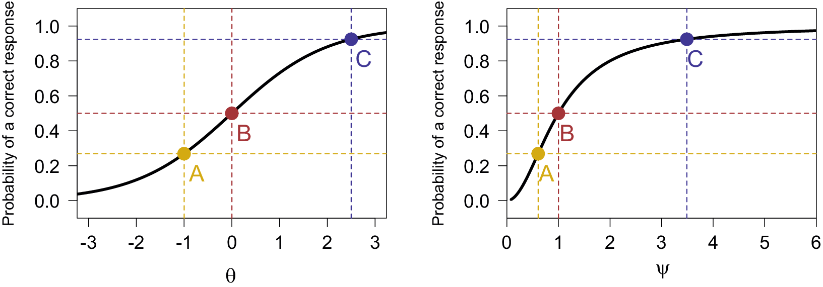
 only represents the response probabilities of persons in a different coordinate system (i.e., a different parametrization). Although the person ordering is preserved (because of the strict monotonicity), the distances between persons are generally altered. This is illustrated graphically in Figure 1 for the Rasch model with
$\psi =e^{ \frac {\theta }{2}}$
 (and thus the inverse transformation
$\theta =2\log (\psi )$
 ).
Two item characteristic curves for a Rasch item (i.e.,
$\alpha =1, \beta =0$
 , and
$c=0$
 ) under two different latent trait parametrizations. In the left panel, the latent trait or person parameter is
$\theta $
 (as in Equation (1)). In the right panel, the person parameter is
$\psi =e^{ \frac {\theta }{2}}$
 . To illustrate the effect of the transformation clearly, we have selected three hypothetical persons (A, B, and C). It can be seen that for both parametrizations, the probability of correctly responding to the item does not change, but the relative positions of the persons on the latent trait do change.

Figure 1 Long description
An item characteristic curve for the Rasch model (i.e.,
 ) under two different parametrizations. In the left panel, the latent trait or person parameter is
 (as in Equation 1). In the right panel, the person parameter is
 . To illustrate the effect of the transformation clearly, we have selected three hypothetical persons (A, B, and C). It can be seen that for both parametrizations, the probability of correctly responding to the item does not change, but the relative positions of the persons on the latent trait do change.
This scale indeterminacy problem (i.e., the lack of a unique scale for the latent trait) has long been recognized in IRT (see, e.g., Ballou, Reference Ballou2009; Feuerstahler, Reference Feuerstahler2019; Lord, Reference Lord1975; Ramsay, Reference Ramsay1996). However, the issue has largely been ignored by relying on the
$\theta $
 scale by convention in most IRT analyses, publications, and software (a “measurement by fiat” approach).
But ignoring a problem does not resolve it and it matters because latent trait scores or person parameter estimates from IRT models are used in secondary analyses that compare groups, evaluate interventions, or support policy decisions. In such contexts, researchers often proceed with the conventional
$\theta $
 scale and rely on parametrization-dependent inferences. The problem does not lie with the IRT model itself, because a given model may be a very good model for the data, but with downstream uses of the person parameter estimates that are not invariant under reparametrizations.Footnote
1
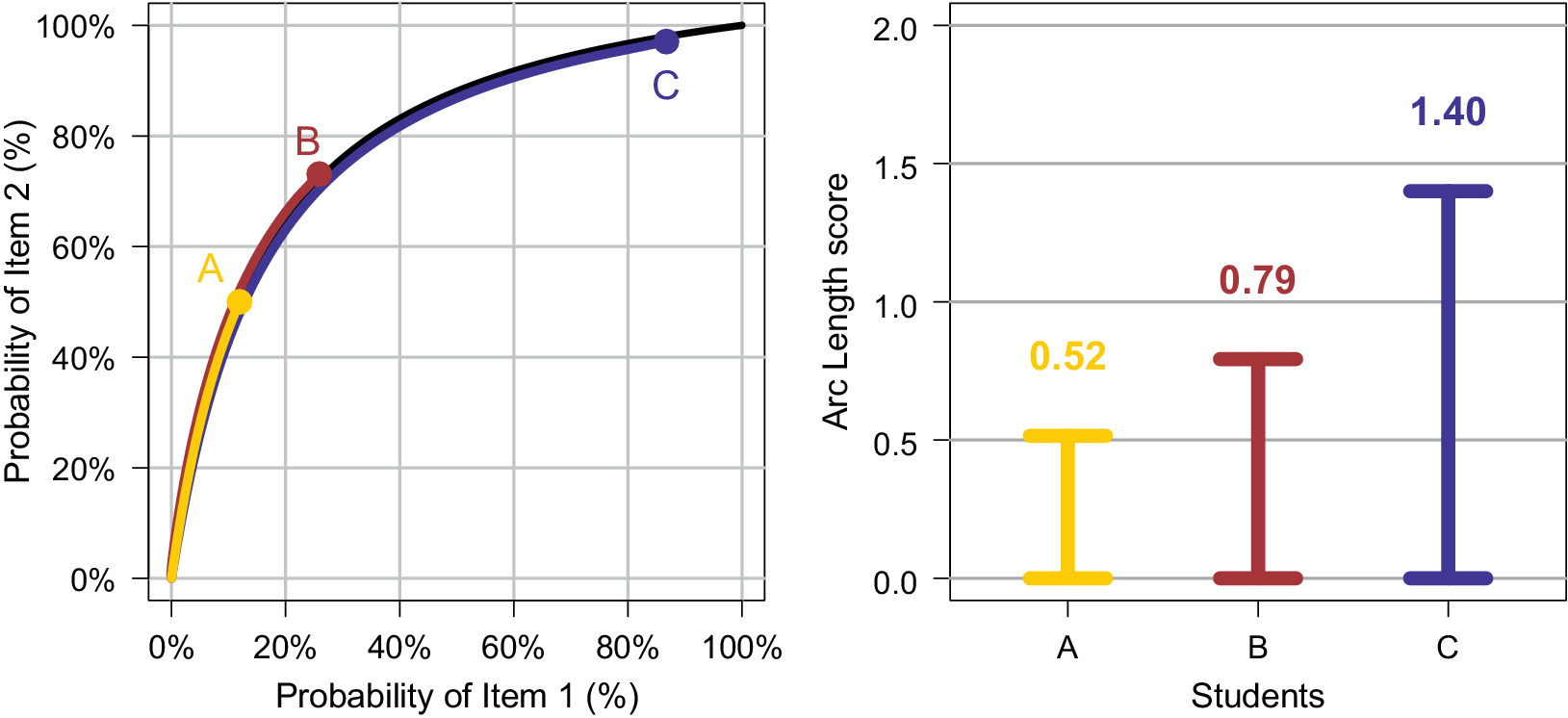
The first (to the best of our knowledge) to address the scale indeterminacy problem using a geometric perspective is Ramsay (Reference Ramsay1996). Because the response probabilities under an IRT model are parametrization-invariant, Ramsay (Reference Ramsay1996) proposes to use these probabilities to define a parametrization-invariant ability measure. Specifically, Ramsay (Reference Ramsay1996) starts from the test performance curve (TPC; see also Ramsay & Wiberg, Reference Ramsay and Wiberg2017), which is the curve defined by the probabilities of correctly solving each test item in a Euclidean space. Thus, if there are m items, then the TPC traces in the m-dimensional unit hypercube a curve defined as
$\text {TPC}(\theta ) =(\pi _1(\theta ),\dots ,\pi _j(\theta ),\dots ,\pi _m(\theta ))$
 . An example with two Rasch items can be seen in Figure 2. Using the TPC, the distance between any two test takers (out of A, B, and C) can be calculated as the length of the path connecting them.
The left panel displays the test performance curve (TPC) in black for a two-item test of Rasch items. The colored lines depict the arc-length scores for three students (A, B, and C). Arc length is measured as the length of the curve from its origin to the student’s position. The right panel presents each student’s computed arc-length scores to facilitate the comparison.

Figure 2 Long description
The left panel displays the test performance curve (TPC) in black for a two-item test of Rasch items. The colored lines depict the arc length scores for three students (A, B, and C). Arc length is measured as the length of the curve from its origin to the student’s position. The right panel presents each student’s computed arc length scores to facilitate the comparison.
The approach of Ramsay (Reference Ramsay1996) leads to an alternative ability measurement for a particular person P, called here arc-length ability and denoted as
$L(P)$
 . The arc length represents the path length or distance along the TPC starting from the origin (where the probability of solving each of the items correctly is zero) to the actual position of person P on the curve. For the 3PL model, the arc length is calculated as follows for a person P with person parameter
$\theta _P$
 :

Ramsay’s arc length
$L(P)$
 is invariant under monotone transformations of the person parameter because it is based entirely on quantities that are invariant under monotone transformations themselves (i.e., the probabilities of solving items correctly).
Despite its conceptual appeal, the arc length has received little attention in psychometric research over the past few decades (but see, e.g., Feuerstahler, Reference Feuerstahler2020, Reference Feuerstahler2023; Rossi et al., Reference Rossi, Wang and Ramsay2002; Sijtsma & Meijer, Reference Sijtsma, Meijer, Rao and Sinharay2006). The reasons for this relative neglect are unclear. One possible explanation is that arc length relies on differential geometry, a branch of mathematics that is not commonly associated with psychometrics and with which many researchers may be unfamiliar. At the same time, the concept may also appear somewhat ad hoc, insofar as it defines a measure by tracking distance along a probability curve. Together, these features may have limited its broader adoption.Footnote 2
In this article, we want to further develop the arc-length approach by providing a firm conceptual foundation. This will require the use of concepts from non-Euclidean differential geometry rather than from classical Euclidean differential geometry. The reason for this shift becomes apparent when reconsidering how distances based on arc length are actually computed. In the approach of Ramsay (Reference Ramsay1996), the distance between two persons (e.g., A and B in Figure 2) is defined as the length of the segment of the TPC connecting their locations, an idea that is intuitively appealing. However, for a specific statistical model (e.g., the Rasch or 3PL model), the TPC can be seen as a family of probability distributions
$p(y \mid \theta )$
 , where
$y = (y_1,\dots ,y_j,\dots ,y_m)$
 denotes the binary response vector and
$\theta $
 the ability parameter (assuming known item parameters). Consequently, the locations of two persons on the TPC correspond to two distinct model instances,
$p(y \mid \theta _A)$
 and
$p(y \mid \theta _B)$
 . Stated differently,
$p(y \mid \theta _A)$
 and
$p(y \mid \theta _B)$
 are two different points in a model space. As shown by Rao (Reference Rao1945) and elaborated in Amari (Reference Amari2016) and Calin and Udrişte (Reference Calin and Udrişte2014), these model instances generally do not just form a curve in Euclidean space as is (implicitly) assumed by Ramsay (Reference Ramsay1996). Rather, these model instances form a curved, non-Euclidean space. (Note that the field of non-Euclidean differential geometrical analysis of statistical models is also called information geometry; see Amari, Reference Amari2016.)
This article makes two contributions. First, we will derive a parametrization-invariant distance for the 3PL and Rasch models, which we call geodesic ability. Crucial in this distance calculation is the Fisher information, which is used to define the Fisher–Rao metric, and then for measuring how different two nearby persons are in terms of their probability distributions implied by the model. Second, we compare the new geodesic ability to Ramsay’s arc-length proposal. Both proposals are motivated by the same concerns but they arise from different geometric structures (Euclidean for Ramsay’s arc length and non-Euclidean for the geodesic ability). As a result, the arc-length and geodesic ability will be similar, but not equal.
The remainder of the article is organized as follows. First, we start by introducing the differential-geometric framework, followed by a derivation of the geodesic ability for the 3PL model. Next, we study the special case of the Rasch model in more detail. We end the article with a conclusion.
2 Non-Euclidean differential geometry
In this section, we will explain briefly the basic notions of differential geometry for statistical models. Interested readers can consult various sources for more information (see, e.g., Amari, Reference Amari2016; Boothby, Reference Boothby1986; Lee, Reference Lee2012; Tu, Reference Tu2010). The relation between statistics and differential geometry is more deeply elaborated in Amari (Reference Amari2016), Calin and Udrişte (Reference Calin and Udrişte2014), Kass (Reference Kass1989), and Kass and Vos (Reference Kass and Vos2011). Two noteworthy papers from quantitative psychology with nice introductions into some of the material used in this article are Ly et al. (Reference Ly, Marsman, Verhagen, Grasman and Wagenmakers2017) and Segert and Davis-Stober (Reference Segert and Davis-Stober2019).
A parametric statistical model can be viewed as a collection
$\mathcal {M}$
 of probability distributionsFootnote
3
,
Footnote
4
(with outcome space
$\mathcal {S}$
 ) indexed by a parameter
$\theta $
 :
$\mathcal {M}= \left \{ p(y|\theta ) \, | \, \theta \in \Theta \right \}$
 (McCullagh, Reference McCullagh2002). The parameter
$\theta $
 can be a scalar (as in the 3PL model from Equation (1)) or, more generally, a vector of dimension k. The set
$\Theta \subseteq \mathbb {R}^k$
 is called the parameter space. The tools in this article require that we are dealing with well-behaving statistical models. By well-behaving, we mean that the model should be well-identified (i.e.,
$\theta \neq \theta ^{\prime }$
 implies that
$p(y|\theta ) \neq p(y|\theta ^{\prime })$
 ) and satisfy general regularity conditions. In addition, if the model is multidimensional, then the Fisher information matrix should be of full rank for all
$\theta $
 . The most common statistical models belong to this class of regular statistical models (e.g., normals with unknown location and scale, exponential family models, etc.).
A regular parametric statistical model
$\mathcal {M}$
 constitutes a smooth (or differentiable) manifold of distributions, which means that an (infinitely) differentiable and invertible map exists from the manifold to the parameter space
$\Theta \subseteq \mathbb {R}^k$
 (such a map is called a chart map or chart). The dimensionality k of the map is the dimensionality of the manifold. For instance, a two-dimensional statistical manifold is illustrated graphically in Figure 3. A smooth manifold of regular statistical distributions is called here a statistical manifold.
Graphical illustration of a smooth two-dimensional statistical manifold
$\mathcal {M}$
 together with a coordinate or parameter space
$\Theta $
 . Each location on the manifold corresponds to a distribution of some family and
$(\theta _1,\theta _2)$
 is a pair of coordinates indexing the distributions. The mapping between
$\mathcal {M}$
 and the parameter space is represented by the black lines.

Figure 3 Long description
Graphical illustration of a smooth two-dimensional statistical manifold
 together with a coordinate or parameter space
 . Each location on the manifold corresponds to a distribution of some family and
 is a pair of coordinates indexing the distributions. The mapping between
 and the parameter space is represented by the black lines.
A simple example is the family of normal distributions
$ \mathcal {M} = \left \{ p(y|\mu ,\sigma ) = N(\mu ,\sigma ) | (\mu ,\sigma )\in \Theta \right \}$
 ,
$\Theta = \mathbb {R}\times (0,\infty ).$
 Here, each pair
$(\mu ,\sigma )$
 determines one probability distribution, so the model is indexed by two parameters and therefore has dimension
$k=2$
 . The mapping that assigns to each distribution in
$\mathcal {M}$
 its parameter values
$(\mu ,\sigma )$
 is a chart, and it provides a coordinate system for the manifold. Since the density of the normal distribution depends smoothly on
$\mu $
 and
$\sigma $
 (all derivatives of
$p(y|\mu ,\sigma )$
 with respect to
$\mu $
 and
$\sigma $
 are continuous), this family forms a smooth statistical manifold. In this case, the manifold can be understood as the collection of all normal distributions, while
$(\mu ,\sigma )$
 gives one particular coordinate system for describing them.
Different parametrizations of the model provide different coordinate systems on the same statistical manifold. For instance, consider the statistical manifold for the univariate normal distribution, which can be parametrized with
$(\mu ,\sigma )$
 (mean and standard deviation), but also with
$(\mu ,\sigma ^2)$
 (mean and variance), or with
$(\mu ,1/\sigma ^2)$
 (mean and precision, as is common in Bayesian statistics). These different parametrizations provide different coordinate systems to distinguish the distributions of the normal statistical manifold, in the same way as there exist different types of 2D geographical maps that distinguish between actual places on the earth. This comparison also makes clear that the manifold (be it the earth or a statistical manifold) and its properties (e.g., curvature and distance between objects) does not depend on the coordinate system or parametrization that is used.
The statistical manifold of the 3PL model with known item parameters from Equation (1) is a one-dimensional manifold. The most common parametrization is based on
$\theta \in \Theta =\mathbb {R}$
 . However, as explained in Section 1, any smooth strictly monotone transformation of
$\theta $
 can be used as well:
$\psi = e^{\frac {\theta }{2}}$
 ,
$\omega =\sqrt [3]{\theta }$
 , etc.
A particular choice of parametrization of the statistical manifold has to be made in order to perform calculations on the statistical manifold. For example, finding the best fitting model (i.e., the point on the statistical manifold best representing the data) requires a particular parametrization that allows for parameter estimation. However, the arbitrariness of the parametrization requires a researcher to think about which quantities are invariant under reparametrization and which are not. As shown in Figure 1, the difference between two persons’
$\theta $
 scores is not parametrization-invariant. Thus, we seek to derive a notion of distance between two persons that is intrinsic to the model’s geometric structure rather than depending on the chosen coordinate system or parametrization.
A first step is to find an expression for an infinitesimal distance between probability distributions. Consider a parametric family of probability densities
$p(y \mid \theta )$
 , where
$\theta \in \Theta $
 (with dimension k), and two nearby points
$\theta $
 and
$\theta + d\theta $
 in parameter space. In the Euclidean parameter space, the squared distance between these points is given by

This expression, however, uses the notion of a distance in a Euclidean space and it does not reflect how easily one can distinguish between different probability distributions in the close vicinity of
$\theta $
 (for an elaboration on this, see, e.g., Myung et al., Reference Myung, Balasubramanian and Pitt2000). Taking this into account (see the derivation in Appendix A), we see that the squared infinitesimal distance between two nearby distributions becomes

where
$g(\theta )$
 is the Fisher information matrix. This squared distance is called the squared line element, or also the Fisher–Rao metric. Equation (3) can be considered a generalization of the well-known Pythagorean theorem for non-Euclidean geometry. In general,
$(ds)^2$
 is not equal to the squared distance in the (Euclidean) parameter space (i.e.,
$\delta ^2(\theta ,\theta +d\theta )$
 ), unless the statistical manifold itself is a “flat” Euclidean space, in which case
$g(\theta )=I_k$
 (the
$k\times k$
 identity matrix) for all
$\theta $
 . In the univariate case, the Fisher–Rao metric is defined as

Remark. The squared line element
$(ds)^2$
 informs us about the local distinguishability between
$p(y|\theta )$
 and its nearby distributions. A more common quantity to assess differences between distributions is the Kullback–Leibler divergence
$D_{KL}$
 . Using
$D_{KL}$
 , the difference of
$p(y|\theta ')$
 from
$p(y|\theta )$
 is

Although
$D_{KL} \geq 0$
 (with equality when
$p(y|\theta )=p(y|\theta ')$
 for all y), it is not symmetric, nor satisfies the triangle inequality, and thus the
$D_{KL}$
 divergence is not a distance. However, when
$\theta '=\theta +d\theta $
 , the quadratic approximation to
$D_{KL}$
 results in

which means that for nearby distributions, the
$D_{KL}$
 divergence is actually carrying the same information as the local distinguishability
$(ds)^2$
 . (This ends the remark.)
Returning to the main argument, the squared line element
$(ds)^2$
 is called the Fisher–Rao metric because Rao (Reference Rao1945) was the first to show that Fisher’s information matrix
$g(\theta )$
 is in fact a so-called metric tensorFootnote
5
that is used to measure distances on a smooth manifold equipped with this metric. A differentiable manifold endowed with such a metric is called a Riemannian manifold in differential geometry. An important property of
$(ds)^2$
 is stated in the proposition below.
Proposition 1. The Fisher–Rao metric is invariant under smooth reparametrizations.
Proof. We will prove this for the univariate case. For a general proof for the parameter vector case, we refer to Calin and Udrişte (Reference Calin and Udrişte2014).Footnote 6
Assume that
$\phi = \phi (\theta )$
 is a smooth reparametrization. This implies that
$\phi (\cdot )$
 is differentiable, one-to-one, and invertible. The inverse transformation is
$\theta =\theta (\phi )$
 .
Let us denote the distribution under the new
$\phi $
 -parametrization as
$p^{\ast}(y|\phi )=p(y|\theta (\phi ))$
 and the Fisher information as
$g^{\ast}(\phi )$
 . Then, we have to show that
$(ds)^2=(ds^{\ast})^{2}$
 .
Because
$g^{\ast}(\phi )=E\left [ \left ( \frac {d\log p^{\ast}(y|\phi )}{d\phi }\right )^2 \right ]$
 , we need an expression for
$\frac {d}{d\phi }\log p^{\ast}(y|\phi )$
 . Using the chain rule, we find that
$\frac {d\log p^{\ast}(y|\phi )}{d\phi } = \frac {d\log p(y|\theta (\phi ))}{d\phi } = \left. \frac {d\log p(y|\theta )}{d\theta } \right |_{\theta =\theta (\phi )} \frac {d\theta }{d\phi }$
 .
Inserting this in the definition of the Fisher information gives (we write an integral over the sample space
$\mathcal {S}$
 , but if
$\mathcal {S}$
 is discrete, the integral should be understood as a summation):

or in shorter (but somewhat sloppier) notation:
$g^{\ast}(\phi ) = g (\theta ) \left (\frac {d\theta }{d\phi }\right )^2$
 . Because the differential
$d\phi $
 transforms as well (but in the opposite way),
$d\phi =\frac {d\phi }{d\theta }d\theta $
 , the squared line element
$(ds^{\ast})^{2}$
 becomes

so the (squared) line element (i.e., the Fisher–Rao metric) does not change.
In the multivariate case, the result generalizes to
$(ds^{\ast})^{2}= d\phi ^\top \, g^{*}(\phi )\, d\phi = d\theta ^\top \, g(\theta )\, d\theta = (ds)^2$
 .
Remark. The line element
$ds$
 is a dimensionless quantity. Let us start with the scalar parameter
$\theta $
 . As is well-known from statistics, the inverse of Fisher information
$g(\theta )$
 is the variance of an estimator for the parameter
$\theta $
 . Therefore,
$[g(\theta )]=[\theta ]^{-2}$
 , that is, the dimension of the Fisher information is equal to the dimension of
$\theta ^{-2}$
 . Because
$(d\theta )^2$
 has dimension of
$\theta ^{2}$
 , it follows that
$[d\theta ]^2=[\theta ]^2$
 . Combining the ingredients gives
$[ds]^2 = [g(\theta )][d\theta ]^2 = [\theta ]^{-2}[\theta ]^{2}=1$
 . Thus,
$(ds)^2$
 is dimensionless, and therefore also
$ds$
 is dimensionless. (This ends the remark.)
A distance on the manifold
$\mathcal {M}$
 between two arbitrary (not necessarily nearby) distributions
$p_a=p(y|\theta _a)$
 and
$p_b=p(y|\theta _b)$
 can then be calculated by defining a path between them and then computing the length of the path (i.e., an arc length on the statistical manifold). In general, the parameter
$\theta $
 has k components. Assume a smooth parametrized curve
$\theta (t)= (\theta _1(t), \dots , \theta _k(t))$
 with
$t \in [0,1]$
 such that
$\theta (0)=\theta _a$
 and
$\theta (1)=\theta _b$
 . The arc length on the manifold
$\mathcal {M}$
 is found by assuming a fine-grained grid along the path and then accumulating the many small line elements
$ds$
 :

Note that for the distance or arc length on the manifold, we use as a symbolFootnote
7
$d_{\theta (t)}$
 to denote that in general the distance depends on the path taken by the curve
$\theta (t)$
 . Another path
$\tilde {\theta }(t)$
 will likely lead to another arc length.
One particular important path is the one with the shortest possible arc length
$d_{\min }$
 , called the geodesic distance:

The corresponding path is called the geodesic curve, denoted here as
$\theta _{\min }(t)$
 :

The geodesic distance is invariant under smooth parametrizations. Moreover, it is a genuine distance (using p, q, and r for distributions): (1)
$d_{\min }(p,q)\geq 0$
 with
$d_{\min }(p,p)=0$
 (non-negativity), (2)
$d_{\min }(p,q) = d_{\min }(q,p)$
 (symmetry), and (3)
$d_{\min }(p,q)+d_{\min }(q,r) \geq d_{\min }(p,r)$
 (triangle inequality) (Lee, Reference Lee2012).
Finding the geodesic curve is in most situations not straightforward and requires the solution to a variational problem (see, e.g., Atkinson & Mitchell, Reference Atkinson and Mitchell1981; Calin & Udrişte, Reference Calin and Udrişte2014; Gelman & Meng, Reference Gelman and Meng1998). For a number of common distributions, these geodesic distances have been derived and can be found in various sources (see, e.g., Atkinson & Mitchell, Reference Atkinson and Mitchell1981; Calin & Udrişte, Reference Calin and Udrişte2014; Miyamoto et al., Reference Miyamoto, Meneghetti, Pinele and Costa2024).
3 Geodesic ability in the 3PL model
Let us now return to the 3PL model. Consider a single person (with unknown ability) taking a test of m items (and known item parameters
$\alpha _j, \beta _j$
 , and
$c_j$
 ). The probability of a particular
$y_j$
 response on a single item j is given by
$\pi _j(\theta )^{y_j} (1-\pi _j(\theta ))^{1-y_j}$
 and the joint probability for the m items is

where
$\pi _j(\theta )$
 is defined in Equation (1). As mentioned above, with known item parameters, the 3PL model is a one-dimensional statistical manifold and thus the Fisher information matrix is a scalar (Lord, Reference Lord1980):

In this context, the Fisher information is also called the test information function (because it gives the amount of information provided about
$\theta $
 by the particular test of m items).
Proposition 2. For the one-dimensional 3PL model with known item parameters, the geodesic distance between two persons located at
$\theta _P$
 and
$\theta _Q$
 (with
$\theta _Q<\theta _P$
 ) is

Proof. Consider Equation (6). On a one-dimensional statistical manifold with squared line element
$(ds)^2=g(\theta )\, (d\theta )^2$
 , the path as the image of the parametric curve
$\theta (t)$
 between
$\theta _Q=\theta (0)$
 and
$\theta _P=\theta (1)$
 has length

Because non-monotone curves will always lead to larger lengths compared to monotone curves, we will only consider the latter and thus
$\frac {d\theta (t)}{dt}>0$
 . The image of these monotone curves is the path connecting
$\theta _Q$
 and
$\theta _P$
 . Moreover, it is safe to state that for the statistical manifold of the 3PL model, there is only one path connecting the points
$\theta _Q$
 and
$\theta _P$
 .
Now, we can do a change of variable
$\theta ' = \theta (t)$
 (so that
$d\theta ' = \frac {d\theta (t)}{dt}dt$
 ), the length is therefore

Remark. Following Atkinson and Mitchell (Reference Atkinson and Mitchell1981), an alternative derivation is possible in the one-dimensional situation: Find a transformation
$\phi = \phi (\theta )$
 , such that the metric of
$\phi $
 is that of a Euclidean space (i.e.,
$(ds)^2=(d\phi )^2$
 with
$g^{\ast}(\phi )=1$
 ). Such a map only exists in general for one-dimensional manifolds, but not for higher-dimensional ones, which makes this method a “trick” that cannot be applied in general.
Thus, we are looking for a parameter
$\phi $
 such that

because
$g^{\ast}(\phi ) =1$
 for all
$\phi $
 . In that case, the geodesic distance between two test takers can be simply computed as
$\phi _P-\phi _Q$
 . Expressing this difference as a function of the familiar
$\theta $
 then gives the solution.
To find the map from
$\theta $
 to
$\phi $
 (i.e.,
$\phi = \phi (\theta )$
 ) so that the result is a Euclidean metric, we start with the requirement that
$g^{\ast}(\phi ) = g(\theta )\, \left ( \frac {d\theta }{d\phi }\right )^2 = 1$
 . Then, taking the square root of both sides and solving for
$\phi $
 gives the result:

The integration constant C will cancel when taking differences between two
$\phi $
 values. (This ends the remark.)
Now that we have an expression for the geodesic distance between two persons P and Q (such that
$\theta _Q<\theta _P$
 ), we can also replace Q with a reference person that has the lowest possible trait score (i.e.,
$\theta _Q \rightarrow -\infty $
 ). Using Equation (8), gives a corresponding distance defined relative to a fixed origin at
$-\infty $
 :

We call
$A(P)$
 the geodesic ability of person P for the given test. To the best of our knowledge, there exists no closed-form solution to this integral.
The interpretation of
$A(P)$
 differs from that of the conventional latent trait value
$\theta _P$
 . Equal increments in
$\theta $
 do not in general correspond to equal statistical separation between persons, because the local geometry varies with
$g(\theta )$
 . By contrast, equal increments in geodesic ability correspond to an equal distance along the 3PL model manifold.
Proposition 3. The geodesic ability A is invariant under smooth reparametrizations of the latent trait.
Proof. Let
$\phi =\phi (\theta )$
 be a smooth transformation. Using Equation (5), the Fisher information expressed as a function of
$\phi $
 satisfies

Therefore,

where the absolute value has been removed because the transformation is monotone. This shows that the distance is unchanged.
Comparing the geodesic ability
$A(P)$
 (Equation (9)) and Ramsay’s arc length
$L(P)$
 (Equation (6)), it can be concluded that the equations are quite similar, but not the same. The difference comes from the fact that in our derivation, we have taken into account the metric of the statistical manifold. However, more detailed comparisons can be made for the Rasch model.
4 Geodesic ability in the Rasch model
We will now consider the special case of the Rasch model (
$\alpha _j = 1, c_j = 0$
 for all j). The geodesic ability becomes

This can be compared to Ramsay’s arc length for the Rasch model:

The formulas are even more similar than for the 3PL model. The only difference is that the terms of the sum under the radical in Ramsay’s arc length are squared.
As for the 3PL model, there exists no closed-form expression for the geodesic ability in the Rasch model. However, we can get more insight by considering a further simplification: Assume that the m items all have difficulty equal to 0. In this case, the geodesic distance between two persons P and Q reduces to (using the subscript 0 to refer to the special case):

Note that this result is actually equal to the geodesic distance between two binomial distributions as derived by Atkinson and Mitchell (Reference Atkinson and Mitchell1981). This should not come as a surprise because, in the equal item difficulty case, the Rasch model with m items reduces to a binomial model (because the success probability is constant).
Similarly to Equation (9), we can set
$\theta _Q \to -\infty $
 to obtain the geodesic ability for person P, denoted now with a subscript 0 as
$A_0(P)$
 . Thus, it simplifies to

It can be seen that
$\lim _{\theta _P \rightarrow -\infty } A_0(P) = 0$
 and
$\lim _{\theta _P \rightarrow +\infty } A_0(P) = \pi \sqrt {m}$
 .
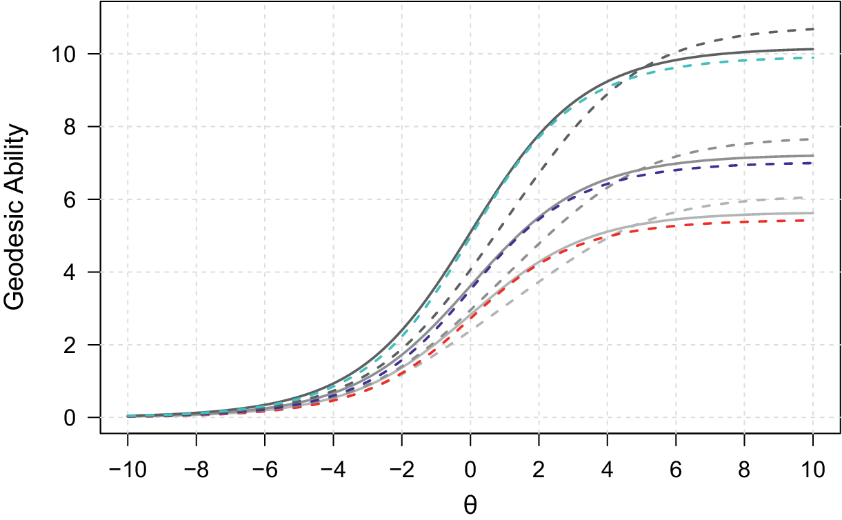
Figure 4 graphically illustrates
$A(P)$
 and
$A_0(P)$
 as functions of
$\theta _P$
 for various choices of
$\beta $
 and number of items m. Several observations can be made from this plot. First, the plots confirm that the geodesic ability starts at 0 and is positive. Second, the major factor that determines where the function levels off is the number of items. Third, if the items are placed symmetrically around zero,
$A_0(P)$
 serves as a decent approximation to
$A(P)$
 .
The geodesic ability
$A(P)$
 (or
$A_0(P)$
 ) as a function of
$\theta _P$
 . The sets of lines with the same color correspond to the same test length:
$m=3$
 (red),
$m=5$
 (blue), and
$m=10$
 (cyan). The dotted lines stand for
$A_0(P)$
 (thus, all item difficulties equal to zero). The solid and dashed lines correspond to tests with item difficulties located symmetrically or asymmetrically around zero, respectively. More specifically, for the solid lines from bottom to top, the following
$\beta $
 values (denoted as
$a(b)c$
 , such that a sequence starts at a, ends at
$c,$
 and has b units between consecutive values) are being used:
$(-1(1)1)$
 ,
$(-1(0.5)1)$
 , and
$(-1(2/9)1)$
 . The dashed lines have asymmetrically placed
$\beta $
 values:
$(-1(2)3)$
 ,
$(-1(1)3)$
 , and
$(-1(4/9)3)$
 .

Figure 4 Long description
The geodesic ability
 (or
 ) as a function of
 . The sets of lines with the same color correspond to the same test length:
 (red),
 (blue) and
 (cyan). The dotted lines stand for
 (thus all item difficulties equal to zero). The solid and dashed lines correspond to tests with item difficulties located symmetrically or asymmetrically around zero, respectively. More specifically, for the solid lines from bottom to top, the following
 values (denoted as
 , such that a sequence starts at a, ends at c and has b units between consecutive values) are being used:
 ,
 ,
 . The dashed lines have asymmetrically placed
 values:
 ,
 ,
 .
Suppose one has to estimate the geodesic ability of a person based on a response vector and known (or calibrated) item difficulties. The standard IRT software can be used to obtain an estimator of
$\theta $
 , denoted as
$\hat {\theta }$
 . Plugging this estimate into Equation (10) gives the estimated geodesic ability:
$\widehat {A(P)}$
 . It is also important to quantify the uncertainty of this estimator. To study this, let us assume again a test of m items with all
$\beta _j=0$
 . Thus, we want to assess the uncertainty of
$\widehat {A_0(P)}$
 . From statistical theory, we know that
$\hat{\theta}-\theta \xrightarrow{D} N\left( 0, g^{-1}(\theta) \right)$
 , where
$g^{-1}(\theta )$
 is the reciprocal of the Fisher information (or, in the multiparameter case, it is the inverse of the Fisher information matrix). Next, we apply the delta method by first computing
$A_0'(P)=\frac {dA_0(P)}{d\theta } = \sqrt {m}\frac {e^{\frac {\theta _P}{2}}}{1+e^{\theta _P}}$
 . This then gives

because if all
$\beta _j=0$
 , then
$g(\theta ) = m\frac {e^\theta }{\left ( 1+e^\theta \right )^2}$
 . Consequently,
$SE\left ( \widehat {A_0(P)} \right ) \approx 1$
 . Hence, we have an estimator with a constant uncertainty. This will not hold exactly for the general
$\widehat {A(P)}$
 , but it can be expected to hold approximately.
It is interesting to note that this result coincides with the findings by Hougaard (Reference Hougaard1982). Based on earlier work, Hougaard (Reference Hougaard1982) studied alternative parametrizations with certain properties. More specifically, for an exponential family model,Footnote
8
the following class of transformations of the canonical parameter
$\theta $
 is considered:

where L is the lower bound for the parameter
$\theta $
 (in our case,
$L=-\infty $
 ) and
$\delta $
 is a constant. The choice of
$\delta $
 determines a new parametrization with a particular property. For example, when
$\delta = \frac {1}{3}$
 , this results in a normal likelihood. The
$\delta =\frac {1}{2}$
 leads to a parametrization with stability of variance. In fact, for
$\delta =\frac {1}{2}$
 , it becomes clear that
$B_{\frac {1}{2}}(\theta ) = A(P)$
 for the Rasch model. Moreover, we have shown the constant variance for the geodesic ability.
5 Conclusion
In this article, we addressed the problem of scale indeterminacy in unidimensional IRT models with known item parameters. Under monotone transformations of the latent trait, the probabilities remain the same, but the scores assigned to persons may be very different. This casts doubt on the use of a person parameter to characterize the ability or latent trait value of an individual.
Using differential geometry, we showed that the Fisher–Rao metric induces an intrinsic distance on the one-dimensional IRT manifold and that this distance gives rise to a corresponding score, geodesic ability
$A(P)$
 . This score is invariant under smooth monotone reparametrizations. Because of this invariance property, the geodesic ability provides a principled alternative to arbitrary latent variables.
The geodesic ability
$A(P)$
 shares some important properties and similarities with Ramsay’s arc length
$L(P)$
 , which has been motivated on the same grounds as the geodesic ability. First, both quantities are derived using a geometrical argument. Second, both ability measures remain invariant under monotone transformations of the latent variable. At the same time, Ramsay’s construction and geodesic ability are not identical. Ramsay’s arc length is defined for a curve embedded in a Euclidean space. Geodesic ability, by contrast, is defined on the statistical manifold of the IRT model using the Fisher–Rao metric. The statistical manifold of the IRT model is a curved space and the geodesic ability takes this curvature into account through the Fisher information. In fact, one could say that the geodesic ability is an intrinsic distance induced by the model itself. Ramsay’s arc length is defined using the TPC. This is a curve in a k-dimensional (Euclidean) space, which acts as an ambient space for the curve. Such an ambient space is not needed in the case of the geodesic ability. The only information needed to calculate a distance is the Fisher information.
The geodesic ability proposed in this article will need some further investigation. One issue that needs to be elaborated is the generalization to multiple dimensions and the corresponding interpretation. Another aspect that deserves further study is the fact that the geodesic ability depends on m, the number of items in the test. A straightforward way of dealing with this problem is to define a normalized version of
$A(P)$
 :
$\frac {A(P)}{m}$
 . This kind of normalization is most likely too crude to work well (since the upper limit of
$A(P)$
 depends on the specific item difficulties), but it may be worthwhile to elaborate further.
The first results obtained from a differential-geometrical analysis for simple unidimensional IRT offer a potential useful way of reconsidering old problems in IRT and latent variable modeling.
Data availability statement
The code for generating most of the figures in this article can be found at https://osf.io/62nqt.
Acknowledgements
This article is the result of follow-up work based on the first author’s presidential address given at IMPS 2019 in Santiago de Chile. Thanks to David Torres Irribara, the associate editor, and the reviewers for constructive comments that have led to a better paper (all remaining errors are the responsibility of the authors). AI was used as a language assistant in this article and to give ideas on how to structure the article.
Funding statement
The research in this article was supported in part by the Research Fund of KU Leuven (C14/23/062) and FWO Research Project (G050826N).
Competing interests
The authors declare none.
Appendix A Derivation of
$(ds)^2 = d\theta ^\top g(\theta )\, d\theta $
 (Equation (3))

In this appendix, we will derive an expression for an infinitesimal distance between probability distributions. For reasons of generality, we will focus on the multivariate case, that is, Equation (3). The derivation follows the original argument of Rao (Reference Rao1945) (see also Caticha, Reference Caticha2022).
To compare the distributions
$p(y \mid \theta )$
 and
$p(y \mid \theta + d\theta )$
 directly, define their relative difference

Using a first-order Taylor expansion,

we obtain

Taking the expectation of
$\Omega (y)$
 with respect to
$p(y \mid \theta )$
 yields

so
$\Omega (y)$
 itself is unsuitable as a distance measure. A meaningful quantity is obtained instead from the expected squared relative difference, which represents the mean squared relative deviation, also called distinguishability, between the two nearby distributions:

The expected value of the product of first derivatives of the log density in Equation (A.2) is the
$(i,j)$
 th element of the Fisher information matrix
$g(\theta )$
 . In matrix notation,

For the statistical models considered in this article, it can be shown
$g_{ij}(\theta ) =-E \left [ \frac {\partial ^2 \log p(y|\theta )}{\partial \theta _i \partial \theta _j} \right ]$
 (see Calin & Udrişte, Reference Calin and Udrişte2014).
The resulting squared line element on the statistical manifold is therefore

This expression generalizes the Euclidean Pythagorean theorem. Only when
$g(\theta ) = I_k$
 for all
$\theta $
 does
$(ds)^2$
 reduce to
$\delta ^2(\theta ,\theta +d\theta )$
 . The derivation also clarifies why the squared relative difference provides a natural starting point for defining distance on a statistical manifold.








 Open access

