1. Introduction
There have been numerous studies of the classical problem of the motion of an interface formed by a heavy fluid lying over a lighter one and stimulated in some way by small perturbations. These studies are often in the context of immiscible fluids (e.g. Freed et al. Reference Freed, Ofer, Shvarts and Orszag1991; Dimonte & Schneider Reference Dimonte and Schneider2000), but very similar phenomena occur for miscible fluids or, indeed, a single fluid containing dynamically significant density gradients (e.g. Voropayev, Afanasyev & van Heijst Reference Voropayev, Afanasyev and van Heijst1993; Dalziel, Linden & Youngs Reference Dalziel, Linden and Youngs1999; Cook, Cabot & Miller Reference Cook, Cabot and Miller2004). In any situation where a low-density fluid region decelerates towards a high-density region (e.g. when a lighter region supports a heavier region against gravity), Rayleigh–Taylor instabilities (RTI) can occur and the resulting interpenetration of fluid parcels and associated mixing can have many consequences. In the geophysical context of flows in atmospheres and oceans, convective overturning in internal wave systems often leads to conditions favourable to such instabilities, and it is well known that this can lead to fully turbulent well-mixed regions. Even the conceptually much simpler situation of instabilities arising on a horizontal interface separating lighter fluid from heavier (above) constitutes a severe test of both numerical and laboratory approaches, as Abarzhi (Reference Abarzhi2010) has pointed out. The internal wave-overturning situation, which contains density and velocity gradients in multiple directions, is much more complicated, and it is not surprising that there are hardly any studies exploring the transition process that precedes the appearance of a fully turbulent mixed region.
Liu et al. (Reference Liu, Bretherton, Liu, Smith, Lu and Rutland2010) have pointed out that ‘in general the breaking of internal waves can be caused by two types of instability’ – i.e. shear-induced Kelvin–Helmholtz (KH) instability or convective instability (leading to RTI). But it seems clear that the initiating instability arising in overturning stationary lee waves in the atmosphere or oceans is generally RTI because of the strong localised vertical density gradients in opposition to gravity, generated by the overturning. This is evident from the work of, for example, Afanasyev & Peltier (Reference Afanasyev and Peltier1998), although they did not specifically name their ‘mushroom-like convective structures’ as RTI fingers, and from Andreassen et al. (Reference Andreassen, Wasberg, Fritts and Isler1994). Both these sets of authors found that full three-dimensional (3D) simulations led to much more rapid breakdown to turbulence than occurs in strictly two-dimensional (2D) cases, so it is clear that the former are required for adequate numerical exploration of the transition processes. Indeed, as will be demonstrated here, provided numerical resolution is sufficient, the Rayleigh–Taylor fingers arising on the strong density shear interfaces (often called plumes and spikes in the literature on the immiscible fluids case) may themselves break down through KH secondary instabilities, and this greatly enhances the evolution to broad-band turbulence.
It is also worth noting some of the literature on propagating waves (as opposed to stationary lee waves) or stratified shear layers, both of which have demonstrated not dissimilar transition scenarios to those less convincingly explored for a stationary breaking lee wave. Fringer & Street (Reference Fringer and Street2003), for example, have studied the breaking of progressive interfacial waves. They showed that 3D instabilities in the form of longitudinal rolls only develop after the initial appearance of the cross-stream billows generated by either a shear or a convective (2D) instability, depending on the interface thickness, and only provided that the regions of static instability within the 2D billows exist for long enough. Troy & Koseff (Reference Troy and Koseff2005) and Barad & Fringer (Reference Barad and Fringer2010) have discussed related scenarios, but also for propagating waves. Similarly, in density-stratified shear layers where, first, (2D) KH billows develop, the route to turbulence subsequently occurs through 3D instabilities, with secondary convective instabilities usually playing a critical role, as shown by Mashayek & Peltier (Reference Mashayek and Peltier2012a ,Reference Mashayek and Peltier b , Reference Mashayek and Peltier2013). Fritts et al. (Reference Fritts, Bizon, Werne and Meyer2003, Reference Fritts, Wang, Werne, Lund and Wan2009) have explored turbulence generation in initial monochromatic propagating waves, contrasting the processes that occur through KH instabilities and breaking gravity waves. We will refer to some of the findings from these authors in our later discussions, as appropriate, but note that all the scenarios differ significantly from that of a steady isolated breaking lee wave.
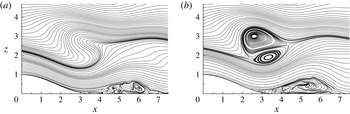
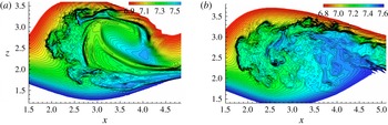
To set the scene, figure 1 shows streamlines on the central vertical plane at
 $y=0$
at two instances in time from computations of linearly stratified uniform velocity (
 $U$
) flow past a Gaussian-shaped hill (height
 $h$
) generating a stationary lee-wave train just downstream and aloft. Once transition is complete, a fully turbulent and essentially steady ‘patch’ (a fully mixed region having largely uniform density) emerges, and the nature of this patch was explored in our previous paper (Yakovenko, Thomas & Castro Reference Yakovenko, Thomas and Castro2011). The hill is 2D but the computation was a full direct numerical simulation (DNS) at
 $\mathit{Re}=Uh/{\it\nu}=4000$
,
 $\mathit{Pr}\equiv {\it\nu}/{\it\kappa}=1$
and
 $F_{h}=U/Nh=0.6$
, where
 $N$
is the Brunt–Väisälä frequency defined by
 $N=[-(g/{\it\rho})(\text{d}{\it\rho}/\text{d}z)]^{1/2}$
. These values of
 $\mathit{Pr}$
and
 $F_{h}$
are typical of situations in both oceans and atmospheres, where large-scale, usually topographically generated, stationary lee waves can occur. In the ocean, dominant density gradients are sometimes generated solely by salt stratification, in which case
 $\mathit{Pr}$
may (equivalently) be up to two or more orders of magnitude higher, but there certainly are situations where breaking waves occur in regions where
 $\mathit{Pr}=O(1)$
or
 $O(10)$
appropriate to thermal stratification in air or water, respectively. On the other hand, the
 $\mathit{Re}$
is much lower than oceanic or atmospheric values, for which typically
 $10^{7}<\mathit{Re}<10^{10}$
. Nonetheless,
 $\mathit{Re}=4000$
is not far from the values in some of the corresponding laboratory experiments (e.g. Castro & Snyder Reference Castro and Snyder1993; Eiff, Huteau & Tolu Reference Eiff, Huteau and Tolu2005) and is sufficient for the breaking lee wave to generate into a fully developed quasi-steady turbulent patch, very similar to those seen in both laboratory experiments and field situations. We discuss the possible influence of
 $\mathit{Re}$
on the transition process in due course.
Streamlines (on the central vertical plane,
 $y=0$
) showing the internal wave (a) prior to (
 $t=17.5$
) and (b) after (
 $t=22.5$
) the start of the transition process. The lee half of the hill is at bottom left and a turbulent separated region, caused by the adverse streamwise surface pressure gradient generated by the lee-wave train, can be seen on the surface downwind of the hill. From Yakovenko et al. (Reference Yakovenko, Thomas and Castro2011).

Throughout this paper we refer to
 $t$
as the appropriately non-dimensionalised time (
 $Ut/h$
) from the start of the computation. The two snapshots in figure 1 were obtained before RTI fingers reach substantial amplitudes and when the flow was still essentially laminar and spanwise-homogeneous. The instability becomes most clearly evident some while after the time when some isopycnals first become vertical (around
 $x=4$
at
 $t\approx 10$
with
 $\mathit{Pr}=1$
). Our interest is to track the transitional process, identifying when and where instabilities first begin to grow (and, in particular, when RTI mushrooms are first evident), exploring their nature and the time-dependent scale of the resulting mixing region, and assessing to what extent the transitional flow differs from the more classical situation of a perturbed horizontal density interface.
Note immediately that this breaking-wave situation is much more complex than the latter more classical case of a perturbed horizontal density interface. In the region around
 $x=2.0,\ z=2.5$
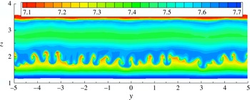
in figure 1(b), for example, there are strong streamwise decelerations of streamwise velocity combined with positive streamwise density gradients, so lighter fluid is being decelerated towards heavier fluid. Likewise, in the same region, the vertical density gradient is positive, against the gravitational acceleration, so, again, lighter fluid is being decelerated towards heavier. There are other regions around the basic (but very temporary) twin-vortex pair generated by the overturning process that contain similar destabilising multiple gradients. The flow is clearly quite unlike the usual cases in which RTI has been studied, but it is not surprising that RTI fingers develop within the strong density shear layers. Figure 2 shows a typical set of density contours some time after the initial development of these fingers. The whole process is explored in detail in § 3 (for
 $\mathit{Pr}=1$
), after the numerical methods used for the computation are briefly described in § 2. Conclusions are summarised in § 4. Subsequent large-eddy simulations (LES) for exactly the same flow but with
 $\mathit{Pr}=700$
(modelling an oceanic or laboratory situation where the stratification is generated solely by salt) will be reported elsewhere, but an initial presentation is given by Yakovenko, Thomas & Castro (Reference Yakovenko, Thomas, Castro and Talamelli2014).
Density contours at
 $t=25$
,
 $x=2.5$
, looking downstream, in the lower strong-shear region bordering what becomes the breaking wave. Notice that the Rayleigh–Taylor mushroom-like structures (‘fingers’) contain regions of low-density fluid (red) brought into the shear layer from aloft by the downward-moving streamlines originating upstream.

2. Numerical methods
The DNS code originated as a finite-difference parallel multi-block Navier–Stokes solver, written in such a way that its efficiency generally increases with the mesh count. The earliest version of the code is described by Thomas & Williams (Reference Thomas and Williams1997), and for density-stratified flows it was modified (when starting the work for Yakovenko et al. (Reference Yakovenko, Thomas and Castro2011)) to include simultaneous solution of the density equation, making the usual Boussinesq assumption. Using coordinates
 $x,y,z,t$
appropriately non-dimensionalised by the obstacle height
 $h$
and, for time, free-stream velocity
 $U$
, the continuity, Navier–Stokes and density equations therefore become
 $$\begin{eqnarray}\displaystyle & \displaystyle \frac{\partial u_{k}}{\partial x_{k}}=0, & \displaystyle\end{eqnarray}$$
 $$\begin{eqnarray}\displaystyle & \displaystyle \frac{\partial u_{i}}{\partial t}+\frac{\partial u_{i}u_{k}}{\partial x_{k}}=-\frac{\partial \hat{p}}{\partial x_{i}}+\frac{1}{\mathit{Re}}\,\frac{\partial ^{2}u_{i}}{\partial x_{k}^{2}}-\frac{{\it\delta}_{i3}}{F_{h}^{2}}\hat{{\it\rho}}, & \displaystyle\end{eqnarray}$$
 $$\begin{eqnarray}\displaystyle & \displaystyle \frac{\partial \hat{{\it\rho}}}{\partial t}+\frac{\partial \hat{{\it\rho}}u_{k}}{\partial x_{k}}=\frac{1}{\mathit{Re}\,\mathit{Pr}}\frac{\partial ^{2}\hat{{\it\rho}}}{\partial x_{k}^{2}}, & \displaystyle\end{eqnarray}$$
 $u,\ \hat{p}$
and
 $x$
have been appropriately non-dimensionalised using
 $U$
, a reference density
 ${\it\rho}_{o}$
(at the domain top) and the obstacle height
 $h$
, and
 $\hat{{\it\rho}}$
has been normalised by
 ${\it\rho}_{o}hN^{2}/g$
. Other quantities are dimensional unless specifically stated otherwise. Here
 $\hat{{\it\rho}}$
and
 $\hat{p}$
represent deviations from the (hydrostatic) reference values, i.e.
 $\hat{{\it\rho}}=g({\it\rho}(x,y,z,t)-{\it\rho}_{o})/({\it\rho}_{o}N^{2}h)$
and
 $\hat{p}=(p(x,y,z,t)-p_{o}-{\it\rho}_{o}gz)/({\it\rho}_{o}U^{2})$
and, for convenience,
 $\hat{{\it\rho}}$
ran from 10 at the bottom of the domain to zero at the top (where
 ${\it\rho}={\it\rho}_{o}$
). The upstream velocity
 $U$
was, again for convenience, set as constant; there is therefore no velocity shear in the initial background field. Here
 $\mathit{Pr}$
is the Prandtl number (equivalent to a Schmidt number if the scalar were viewed as a density-changing contaminant like salt, for example), characterising the ratio between the momentum and thermal diffusivities,
 $\mathit{Pr}={\it\nu}/{\it\kappa}$
. Its value is of the order of unity in air and around 700 in salt water. In oceanic regions, where both thermal (
 $\mathit{Pr}\approx 7$
) and salt (
 $\mathit{Pr}\approx 700$
) stratification are important, it would be necessary to solve the separate equations for both density and salt concentration, but there are situations where either one or the other is dominant. The current computations (with
 $\mathit{Pr}=1$
) are perhaps most relevant to atmospheric scenarios. The last term in (2.2) is the buoyancy term, and the only non-zero contribution appears in the vertical momentum equation, of course, through the gravitational vector. Full details of the numerical methods used are provided in the companion paper (Yakovenko et al.
Reference Yakovenko, Thomas and Castro2011), so here only a brief summary is given.
Second-order central differencing on a uniform Cartesian mesh was applied to all spatial derivatives and a second-order Adams–Bashforth scheme was used for time advancement, with a projection method for pressure computations. A fairly crude immersed boundary method was used to represent the topography: a body force term was added to the right-hand side of (2.2) and used for all cells within the bounding surface of the obstacle. This drag term was of the general form
 $$\begin{eqnarray}F_{i}=-Au_{i}(u_{k}u_{k})^{p/2}\end{eqnarray}$$
and suitable values for
 $p$
(0) and
 $A$
(1000) were chosen on the basis of an optimisation process. The term was applied within a bottom boundary shape, which, for the work described in this paper, was of 2D form and defined by
 $$\begin{eqnarray}\displaystyle & \displaystyle z_{m}=0.5\left[1+\cos \left({\rm\pi}x\frac{h}{L}\right)\right],\quad \text{at }|x|\leqslant L/h, & \displaystyle\end{eqnarray}$$
 $$\begin{eqnarray}\displaystyle & z_{m}=0,\quad \text{at }|x|\geqslant L/h, & \displaystyle\end{eqnarray}$$
 $x=y=0,\ z=z_{m}=1$
defines the location of the hill summit.
For the long-time computations of the turbulent patch arising as a result of wave breaking, and since very fine resolution was required for successful simulation of the transition processes (and the subsequent turbulent patch characteristics), it was necessary to use sponge zones so as to avoid having very large domain lengths (recall that the code used uniform grids).
Flows with wave breaking almost inevitably contain, in addition to the downstream waves, upstream-propagating modes. For any sensibly sized computational domain, these would normally arrive at the upstream boundary before the wave breaking and subsequent turbulent patch has fully developed. A straightforward sponge zone technique was used to prevent long-wave reflections from the two ends of the computational domain. These are fully described and validated by Yakovenko et al. (Reference Yakovenko, Thomas and Castro2011), but their use was less crucial for the current work because transition in the breaking wave occurred at relatively early times. Periodicity was used for the spanwise boundary conditions. The top and bottom domain boundary conditions represented typical towing tank experiments, as fully described by Yakovenko et al. (Reference Yakovenko, Thomas and Castro2011). These entailed a moving wall condition at the top of the domain (
 $z=10$
), an implicit no-slip (and zero scalar flux) condition on the obstacle surface, with free-slip conditions on the rest of the bottom surface (
 $z=0$
).
The results presented in the following sections were obtained using an overall domain size of
 $100h\times 10h\times 10h$
in the streamwise, spanwise and vertical directions, respectively, with a 2D cosine hill having
 $L/h=3.56$
(see (2.5)) centred half-way between the domain boundaries at
 $x=0$
. The sponge zones were located between
 $x_{I}\leqslant x\leqslant x_{SI}$
and symmetrically at
 $x_{SE}\leqslant x\leqslant x_{E}$
(near the downstream and upstream boundaries, respectively), each having a
 $25h$
-long region of cosine sponge strength
 ${\it\sigma}(x)=0.5A_{w}\{1+\cos [{\rm\pi}(x-x_{I})/(x_{SI}-x_{I})]\}$
and
 ${\it\sigma}(x)=0.5A_{w}\{1+\cos [{\rm\pi}(x-x_{E})/(x_{SE}-x_{E})]\}$
, with
 $A_{w}=0.4$
,
 $x_{E}=-x_{I}=50$
and
 $x_{SE}=-x_{SI}=25$
.
The hill’s streamwise length,
 $L/h=3.56$
, was close to the theoretical dominant lee-wave wavelength at
 $F_{h}=0.6$
, which is
 $l/h=3.84$
, so provides effective topographical tuning. The hill also has a maximum slope of
 $20^{\circ }$
, close to the
 $21^{\circ }$
of the Gaussian hills used by Eiff & Bonneton (Reference Eiff and Bonneton2000) and Gheusi, Stein & Eiff (Reference Gheusi, Stein and Eiff2000). The Reynolds number of 4000 was chosen because significantly smaller values gave no wave overturning (for
 $\mathit{Re}\leqslant 100$
) or weaker wave-breaking effects with later and shorter periods of a fully developed mixed region and clear indication of long-term periodic behaviour with quite long relaminarisation periods, as in the DNS of Gheusi et al. (Reference Gheusi, Stein and Eiff2000) at
 $\mathit{Re}=200$
. On the other hand, Reynolds numbers much in excess of 4000 would have required even finer meshes. Effects of Froude number were examined in some initial coarse-grid runs (without sponge layers) with axisymmetric hills at
 $L/h=1.78$
and
 $\mathit{Re}=100$
. However, the maximum wave slope was the largest for
 $0.6\leqslant F_{h}\leqslant 0.7$
and the value
 $F_{h}=0.6$
was chosen; for a 2D hill of any shape this is always below the critical value for wave breaking, as shown by Castro & Snyder (Reference Castro and Snyder1993), and was the value used by Eiff & Bonneton (Reference Eiff and Bonneton2000) and Gheusi et al. (Reference Gheusi, Stein and Eiff2000).
Meshes had node numbers of
 $5120\times 512\times 512$
(
 $1.34\times 10^{9}$
nodes), giving cell sizes of
 ${\rm\Delta}x={\rm\Delta}y={\rm\Delta}z=0.02h$
, which was about three times the minimum Kolmogorov scale (i.e.
 $3.0{\it\eta}$
) within the turbulent patch – more than adequate for a well-resolved DNS of the latter. This is explained fully in Yakovenko et al. (Reference Yakovenko, Thomas and Castro2011). Note that the Kolmogorov scale
 ${\it\eta}$
was estimated using the maximum value of the dissipation
 ${\it\epsilon}$
in the turbulent patch, obtained by time and spatial averaging of the usual relation containing the fluctuating strain tensor, and that mesh sizes of
 $5{\it\eta}$
are usually reckoned to provide adequate resolution (Kim, Moin & Moser Reference Kim, Moin and Moser1987; Barri et al.
Reference Barri, El Khoury, Andersson and Petterson2010). The run was performed with
 $\mathit{Re}=Uh/{\it\nu}=4000$
,
 $\mathit{Pr}=1$
and
 $F_{h}=0.6$
and used a (non-dimensional) time step of
 ${\rm\Delta}t=0.0005$
, satisfying the Courant number restrictions arising from the advection and ‘drag’ terms. This value is, however, much smaller than the Kolmogorov time scale. To address the same problem but with the much larger
 $\mathit{Pr}$
appropriate to (at least some) oceanic applications would, of course, be extremely demanding for DNS. (We have performed some genuine LES for
 $\mathit{Pr}=700$
with an appropriate subgrid scale model but these are not presented in this paper, although a salient result will be mentioned later.) Simulations proceeded for a total non-dimensional time extending to
 $t\approx 60$
but the present paper explores only the transitional stage (i.e. up to
 $t\approx 32$
). (The fully developed turbulent patch that emerges was discussed in our earlier paper (Yakovenko et al.
Reference Yakovenko, Thomas and Castro2011).)
3. Transition processes
3.1. The early stages
In order to promote the transition, avoiding unnecessarily long computational times, the flow field was seeded at
 $t=7.5$
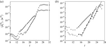
by the addition (to the entire flow field) of white-noise density fluctuations with an amplitude of 2 % of the background density change over the hill height (as explained in Yakovenko et al. (Reference Yakovenko, Thomas and Castro2011)). All modes of this initial perturbation at first decayed, because of the stabilising influence of the density gradient and viscosity, but then provided sufficient residual energy to seed the transition process. Figure 3(a) shows the growth of the density and streamwise velocity fluctuations averaged over the entire span and over a rectangular (
 $x,z$
) region where the internal wave breaks and within which transition begins. (Angle brackets denote averaged values throughout the paper, although the nature of the averaging is not always the same.) It is clear that there is exponential growth in
 $\langle u^{\prime 2}\rangle$
over a time range of about
 $16<t<22$
, with a somewhat smaller range in the case of
 $\langle \hat{{\it\rho}}^{\prime 2}\rangle$
. Such growth is expected for an initial linear instability process. The variances grow by at least two orders of magnitude during this time or, if averaging is restricted to a spanwise line average, up to five orders of magnitude. Figure 3(b) shows the same quantities but averaged only along the span and at a specific
 $x,z$
location. Notice that, at least for
 $\langle u^{\prime 2}\rangle$
, there is a distinct ‘blip’ in the exponential growth around
 $t=21$
; this is because of the slow but small shift in the whole wave-breaking region, making line-averages very dependent on their precise
 $x,z$
location and thus perhaps less useful for diagnostic purposes.
Growth of density and streamwise velocity fluctuations. (a) Spatially averaged over the span and within a box defined by
 $1.25\leqslant x\leqslant 5$
,
 $1.25\leqslant z\leqslant 3.75$
. (b) Averaged over the spanwise line at
 $x=2.5$
,
 $z=2.0$
. Symbols: open circles,
 $\langle \hat{{\it\rho}}^{\prime 2}\rangle$
; open triangles,
 $\langle u^{\prime 2}\rangle$
; solid circles, density variance,
 $\langle \hat{{\it\rho}}_{1}^{\prime 2}\rangle$
, of the lowest wave mode supported by the system.

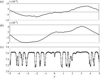
Inspection of the spanwise density variations shows that it is growth in the first mode (with a wavelength of the domain width) that dominates, as illustrated by the density profiles shown at two representative times (
 $t=18$
and 20) in figure 4. Velocity perturbation profiles have a very similar character. Fitting a single sine wave to these and other profiles, with an appropriate (but inevitably very approximate) choice of phase and amplitude in each case, allows an estimate of the variance,
 $\langle \hat{{\it\rho}}_{1}^{\prime 2}\rangle$
say, of the first mode alone. The results are included in figure 3(b), and it is clear that the smaller-wavelength modes contribute very little to the total growth in these early stages. Note that these modes do not grow proportionally as much as the first mode (see below), so that the profile in figure 4(b) is less ‘wiggly’ than that in figure 4(a). Only towards the very end of this period (i.e.
 $t>22$
) does there begin to be any visible evidence of the mushroom-type structures (as seen in figure 2, for example) usually associated with the development of RTI in more classical cases. Spanwise spectra, although noisy (and thus not shown), nonetheless indicate the presence of lower-wavelength modes, but these are hardly amplified and may indeed continue to decay over much of the field because of the predominantly stable stratification. Like the dominant spanwise wave mode, they appear almost as soon as a region of unstable density gradient appears, as is clear from the visualisations discussed below.
Spanwise density (
 $\hat{{\it\rho}}$
) profiles at
 $x=2.5$
,
 $z=2$
at (a)
 $t=18$
, (b)
 $t=20$
and (c)
 $t=25$
. Panels (a) and (b) show
 $\hat{{\it\rho}}^{\prime }$
, the fluctuations about the spanwise mean; panel (c) shows
 $\hat{{\it\rho}}$
, the absolute values.

Density contours on
 $y=0$
(the central plane) in the lee of the obstacle, showing the developing primary breaking region: (a)
 $t=8$
; (b)
 $t=10$
; (c)
 $t=12$
; (d)
 $t=14$
; (e)
 $t=18$
; ( f)
 $t=20$
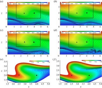
. The rectangular box in panels (a)–(d) delineates the region over which averages (in figure 3
a, for example) were obtained. The black triangle identifies the location where the line averages of figure 3(b) were obtained. Note the expanded scale used for panels (e) and ( f); the box in these two plots is approximately the size of the figures themselves so is not shown.

Figure 5 shows density contours in the lee of the obstacle on the spanwise centreline, at different times. Instantaneous streamline plots look essentially identical. The seeding white noise remains just visible as random ‘wiggles’ in each contour (when the views are magnified), although as noted earlier its amplitude decays rapidly because of the initial stabilising density gradients everywhere. By
 $t\approx 10$
(figure 5
b), however, the density field has developed its first small region of unstable gradient, around
 $x=4,\ z=2$
. Figure 6(b), which shows density contours at
 $t=10$
in a spanwise plane at
 $x=4$
, shows some clear spanwise structure, visible above the background noise level. The visualisation suggests a dominant wavelength in the region
 $(0.3{-}0.5)h$
. The most unstable wavelength can be estimated from its classical value for perturbations with multiple wavelengths (as here) applied to a plane boundary between two incompressible fluids of different densities
 ${\it\rho}_{1}$
and
 ${\it\rho}_{2}$
(e.g. Taylor Reference Taylor1950; Youngs Reference Youngs1984). This is given by
 ${\it\lambda}_{m}=4{\rm\pi}{\it\nu}^{2/3}(gA_{t})^{-1/3}$
, where
 $A_{t}$
is the Atwood number measuring the relative size of the density difference,
 $A_{t}=({\it\rho}_{1}-{\it\rho}_{2})/({\it\rho}_{1}+{\it\rho}_{2})$
. For the present case, this expression can be reformulated as
 $$\begin{eqnarray}\frac{{\it\lambda}_{m}}{h}=4{\rm\pi}\left(\frac{F_{h}^{2}}{\mathit{Re}^{2}}\frac{2{\rm\Delta}{\it\rho}_{h}}{{\rm\Delta}{\it\rho}}\right)^{1/3},\end{eqnarray}$$
where
 ${\rm\Delta}{\it\rho}_{h}$
is a reference density change over the height of the obstacle and
 ${\rm\Delta}{\it\rho}$
is the density change over the unstable density gradient region. This result refers to the simple (thin and horizontal) density interface case, so comparisons with the present rather more complicated case should perhaps be viewed with caution. However, given that alternative expressions for cases more similar to the present are not available, it is worth making such a comparison. It is not obvious what should be used for
 ${\rm\Delta}{\it\rho}$
when the unstable region first appears. However, close inspection of the vertical density profile at
 $x=4$
(for
 $t=10$
) suggests that a (normalised)
 ${\rm\Delta}{\it\rho}$
of approximately 0.001 represents the difference between maximum and minimum density in the (small) unstable region and this value yields
 ${\it\lambda}_{m}/h\approx 0.45$
, which is not too inconsistent with what is implied by the visualisation of the spanwise structure in figure 6(b).
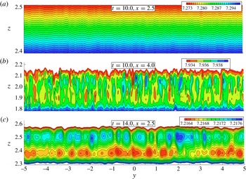
Density contours in vertical slices across the span (i.e.
 $-5\leqslant y\leqslant 5$
) at
 $t=10$
and 14 and two
 $x$
locations. Note the different
 $z$
-axis scales, each greatly expanded compared with the
 $y$
-axis scale, and the varying density scales. Both were carefully chosen to allow the structures to be visually clear.

At this time (
 $t=10$
) density contours at
 $x=2.5$
(figure 6
a) do not indicate any structure above the random background noise. Note that the density scale is much less amplified in this figure than in figure 6(b), but increasing the amplification merely yields a picture of random noise. By
 $t=14$
, however, the convective overturning has developed to the point where there is a region of positive vertical density gradient around
 $x=2.5$
, as shown in figure 5(d). Spanwise structure is thus beginning to be evident there, as indicated in figure 6(c), and at
 $x=4$
it has further developed from the state shown in figure 6(b). It is emphasised, however, that the amplitudes are very small; figure 6(b) shows contours covering a density range of only approximately 0.6 % of the upstream density change over the height of the topography. It is therefore quite difficult to visualise the structures clearly above the remaining background white noise.
(a) Density contours (for
 $\mathit{Pr}=1$
) in the (
 $y{-}z$
) plane at
 $x=2.5$
and
 $21.0\leqslant t\leqslant 24.5$
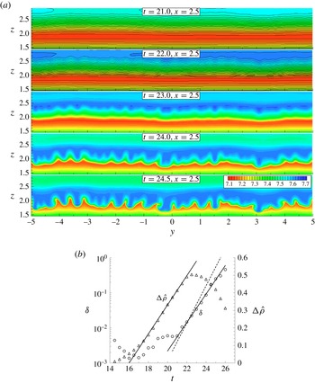
(top to bottom). (b) Growth of mixing height
 ${\it\delta}$
(○) and density difference
 ${\rm\Delta}\hat{{\it\rho}}$
(▵) at
 $x=2.5$
.

The exponential growth of the first mode continues to about
 $t=22$
, after which it saturates and the growth of the higher-order (smaller-wavelength) modes typical of the subsequent RTI structures proceeds much more rapidly, so that spanwise density variations become dominated by the latter. This is explored in § 3.2, but a preview is given in figure 4(c). This shows not only the greatly increased size of the density variations across the span at
 $t=25$
(a 0.5 difference between minimum and maximum values, compared with less than 0.01 at
 $t=20$
, figure 4
b), but also the lack of any dominant low-wavenumber mode of the kind that prevails at earlier times. By comparing figure 4(c) with figure 2, the large mushroom-like excursions of lower-density fluid originating in the lower regions (where such fluid ends up after the large-scale overturning process) are clearly evident.
In classical cases of RTI development, it is common to consider the growth of the thickness of the mixed region,
 ${\it\delta}$
say, which is expected to be exponential during the linear development phase before the RTI structures begin to merge. It is therefore of interest in the present case to attempt to quantify how this mixed layer thickness varies with time. As an example, we consider the situation at
 $x=2.5$
. Density contours in the vertical plane at that location are shown in figure 7(a), for
 $21<t<24.5$
. Note that the particular
 $z$
region shown initially has heavier fluid overlaying lighter. A suitable measure of the mixing height at a given
 $t$
was computed using a three-stage process. First, the spanwise averages of the local minimum and maximum densities (
 $\langle \hat{{\it\rho}}_{min}\rangle$
and
 $\langle \hat{{\it\rho}}_{max}\rangle$
) along vertical lines in the region containing a positive vertical density gradient were determined. Second, we computed the spanwise averages of the minimum and maximum levels (
 $\langle z_{min}\rangle$
and
 $\langle z_{max}\rangle$
, say) in the distribution of levels (
 $z_{0.5}(y)$
) where the density is half-way between its (averaged) minimum and maximum values (i.e. where
 $\hat{{\it\rho}}=\langle \hat{{\it\rho}}_{min}\rangle +{\textstyle \frac{1}{2}}{\rm\Delta}\hat{{\it\rho}}$
, with
 ${\rm\Delta}\hat{{\it\rho}}=\langle \hat{{\it\rho}}_{min}\rangle -\langle \hat{{\it\rho}}_{max}\rangle$
). Finally, the mixing height was defined as
 ${\it\delta}=\langle z_{max}\rangle -\langle z_{min}\rangle$
. Small-scale wiggles in the density field (arising from the initial random noise) were largely filtered out by first (i.e. before the search for the local minimum and maximum values) performing sub-averaging of
 $z_{0.5}(y)$
over a small number of spanwise nodes. Note that this mixing height is not exactly the same as the true mixing thickness, for the layer is actually inclined to the vertical, as explained later. At
 $x=2.5$
true layer thicknesses can be taken as smaller by a factor of approximately 1.4 than the vertical height
 ${\it\delta}$
shown in figure 7(b), which plots the variations with
 $t$
of both
 ${\it\delta}$
(obtained with nine-node sub-averaging) and
 ${\rm\Delta}\hat{{\it\rho}}$
.
Growth in the mixing region height (
 ${\it\delta}$
) is initially non-monotonic but subsequently becomes exponential beyond
 $t=21$
until
 $t\approx 25$
, just as expected for the initial linear stage of the instability, before the clear mushroom-like structures emerge. This latter nonlinear stage, beyond
 $t\approx 21$
, corresponds to the non-merging growth of RTI mushrooms, as illustrated by the density contours shown in figure 7(a) and as will also be shown in the following section. Once the density difference,
 ${\rm\Delta}\hat{{\it\rho}}$
, across the unstable region at
 $x=2.5$
has reached approximately 0.1 at
 $t=17$
, it grows linearly until about
 $t=22$
(figure 7
b), owing to the interpenetration of the ‘tongues’ of heavier and lighter fluid during the on-going large-scale wave overturning. Although this time range roughly matches that over which there is exponential growth in density and velocity variances (figure 3
b), these two facts should not be seen as connected. As shown earlier, the latter is a result primarily of the first mode of the general wave system responding to the topographic forcing. Saturation of this first mode is perhaps at least partly a result of the rapidly growing, much smaller-scale, RTI mode for
 $t>22$
(see figure 7
a and below) extracting an increasingly large proportion of the available energy for instability growth. These variations in
 ${\it\delta}$
and
 ${\rm\Delta}\hat{{\it\rho}}$
are very typical; they can be seen – with appropriate time shifts – at other streamwise locations (like
 $x=4$
, where an unstable density gradient first appears). Indeed, as the large-scale overturning proceeds, the appearance of the small-scale structure with wavelengths around
 $(0.3{-}0.5)h$
moves gradually upstream (from
 $x=4$
) in concert with the upstream-expanding region of positive vertical density gradient. This was concluded from inspection of similar data (density fields, spectra, etc.) obtained at other streamwise locations.
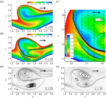
(a,b) Density contours on
 $y=0$
(as for figure 5) at (a)
 $t=22$
and (b)
 $t=25$
. (c) An expanded version of part of the field shown in panel (b). (d,e) Streamlines on
 $y=0$
at (d)
 $t=22$
(i.e. just before the plot in figure 1
b) and (e)
 $t=25$
. The large bold arrows indicate the flow direction far upstream, and the vertical dashed lines in panel (c) mark the slices seen in
 $y{-}z$
views in figure 11.

It should be emphasised that it is the single large-scale overturning roll (in the
 $x{-}z$
plane) that leads to statically unstable density interfaces and thence to the RTI on those interfaces. This (spanwise) roll is quite different from any longitudinal convective rolls, like those seen by Fritts, Isler & Andreassen (Reference Fritts, Isler and Andreassen1994) but not seen in the present flow. It arises because of the linear wave field being continuously forced by the topography.
3.2. The late stages – beyond
 $t=22$
; flow visualisation

We begin discussion of the later stages of transition by showing, in figure 8(a–c), density contours on the central plane at
 $t=22$
and 25. In this (and all plots of density contours) red and blue denote light and heavy fluid, respectively. At
 $t=22$
the incursion of a tongue of heavy fluid into the centre of the wave-breaking region has increased in size and strength considerably from the situation at
 $t=20$
shown in figure 5( f). Figure 8(d) is a plot of the instantaneous streamlines at that time; note the twin vortex that has developed, with temporary stagnation points around
 $x=2.5$
,
 $z=1.8$
and
 $x=4.3$
,
 $z=2.5$
. At this stage the flow remains essentially laminar and 2D, and these views of the twin vortex are independent of spanwise position, apart from very slight shifts because of the amplified first mode discussed earlier. The leading ‘bulb’ of the (heavy) density tongue, generated by the bottom part of the large-scale wave being swept upwards and then backwards (upstream), subsequently splits into two, with one part moving up and the other moving down and, as they do so, extending downstream; this is illustrated by the situation at
 $t=25$
, in figure 8(b). Meanwhile, the baroclinically generated (spanwise) vorticity produced around the stagnation region enhances this split interface as it is convected around by the velocity field. Figure 9, which shows vorticity contours at
 $t=25$
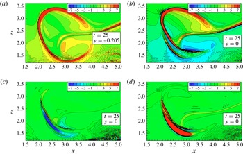
and is discussed later, emphasises this. It is possible in figure 8(b) to see the imprint in this
 $x{-}z$
plane of a mushroom structure that appears on the curved density interface between heavy and light fluid, which runs from near the stagnation point (around
 $x=2.5$
,
 $z=2$
) to around
 $x=4$
,
 $z=1.5$
. Figure 8(c) is an expanded version of figure 8(b), showing a little more detail of this interface for
 $x<3$
.
(a) Total vorticity contours on the
 $y=-0.2$
plane at
 $t=25$
; (b–d) the
 $y$
,
 $z$
and
 $x$
components of vorticity, respectively, on
 $y=0$
.

These figures for
 $t=25$
might, alternatively, suggest at first sight that around the breaking wavefront there are multiple layers of alternating light and heavy fluid. Moving vertically up the line defined by
 $x\approx 2.5$
, for example, three subsequent maxima in density are evident in figure 8(c) below
 $z=2.2$
, say, with lower-density regions between them. Such ‘multiple layers’ have been noted before (Voropayev et al.
Reference Voropayev, Afanasyev and van Heijst1993; Afanasyev & Peltier Reference Afanasyev and Peltier1998), but much less clearly delineated. However, this would be the wrong conclusion. On the one hand, the local maximum around
 $z=1.7$
is not evidence of a layer, but simply a result of vertical interpenetration of two parts of an RTI mushroom structure on a folding interface, which have grown in scale significantly by that
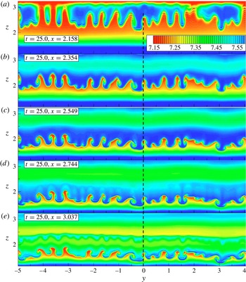
 $x,z$
location and contain an expanding blob of heavier fluid (the mushroom ‘hat’) moving downwards, with some areas of relatively lighter fluid just above it at some spanwise sections (like
 $y\approx 0$
) but not in others. Close inspection of the vertical line at
 $y=0$
,
 $x=2.55$
in figure 11 (or figure 2) clarifies this. On the other hand, the interfaces above
 $z=1.8$
between lighter and heavier fluid do represent thin layers, resulting from the initial thin tongue of returning fluid (visible in figures 5
e, f and 8
a), which splits into two as described above.
This point is further clarified in figure 9, which shows vorticity contours at
 $t=25$
, in terms of both the total vorticity magnitude (figure 9
a) and the three individual vorticity components (figure 9
b–d). Within the mushrooms, the inclined structures produce
 $x$
- and
 $y$
-component vorticity, so figure 9(c,d) shows these components being strongest in the region between the two edges of the folded-over interface evident in figure 9(b) (and figure 8
c). The thickness of the high-vorticity region is strongly dependent on the precise spanwise location of the viewing plane, as is evident by inspecting the location of the RTI structures in figure 2 (and figure 11
c), for example. At
 $y=0$
the slice cuts through the mushroom structure, whereas at
 $x=-0.2$
it does not – hence the difference between figures 9(a) and 9(b–d). Note that in figure 9(a,b) some small-scale features are apparent both upwind and downwind of the bottom of the breaking-wave region. These could be gravity waves (or perhaps numerical artifacts propagating from the high-velocity very thin shear layers near the obstacle surface), but they are not relevant to the transition process itself. Note also that the vortex features apparent in the instantaneous streamlines shown in figure 8(d) are relatively weak motions (the vorticity within the body of the rotors, seen in figure 9, is very low compared with that around the edges). The rotors are thus not dynamically significant compared with the curved vorticity and density sheet surrounding the breaking region on which the RTI develops (see below).
Sketch of the flow structure at late stages (
 $t>23$
), when RTI perturbation amplitudes become substantial. (a) A 2D view from the side, which may be compared with, for example, figures 8 and 9. Bold dashed lines indicate the strongest density interface regions. Solid (lighter) lines with arrows indicate flow direction; the straight, bold arrows indicate major regions of deceleration in the
 $x$
and
 $z$
directions; plus and minus signs indicate heavy and light fluid, respectively. The most unstable region susceptible to RTI is highlighted by the shaded ellipse. (b) An ‘extruded’ view showing the ‘open cylinder’ of strong density interface across the span; the lighter dashed wavy line along the span indicates the RTI mode and includes loci of three sample wave peaks. The axes’ coordinate origin
 $(0,0)$
is indicated in panel (a), but distances are only approximate and the
 $z$
scale is expanded somewhat.

Density contours at
 $t=25$
from (a)
 $x=2.16$
to (e)
 $x=3.04$
. The vertical dashed line marks the
 $y=0$
slice, seen in an
 $x{-}z$
view at
 $t=25$
for
 $x=2.55$
in figure 8(c), which, in turn, indicates some of the
 $x{-}y$
sections seen in this figure.

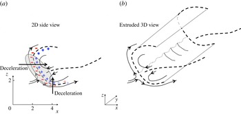
A helpful way to visualise all this is provided by the sketch in figure 10, which can be compared with figures 8 and 9. The central ‘tongue’ of recirculated heavy fluid weakens after it has split, and the strongest interface, enhanced near the front of the breaking region by baroclinically generated vorticity, then eventually forms (topologically) an open-sectioned cylinder running across the entire span. This cylinder is not exactly straight – as noted earlier, there is a large-wavelength spanwise perturbation of the whole structure, not shown on the sketch (and perhaps of Crow type, see later). RTI first occurs, as expected, in the regions where the flow is most strongly decelerated against a positive density gradient. This is shown by the shaded ellipse in figure 10(a), which contains the stagnation region and a mix of regions between those where the strongest density gradient is horizontal (near the front, just above the stagnation point, and accompanied by streamwisely decelerating fluid) and vertical (around the bottom and in the direction of the gravity vector). The Rayleigh–Taylor perturbation constitutes a spanwise short-wavelength perturbation on the curved (‘cylindrical’) density interface, shown by the wavy dotted line running spanwise in figure 10(b), and the resulting regions of significant vorticity (along the individual mushroom edges) are stretched on that interface, as described above. The RTI activity during the nonlinear stage thus results in an array of counter-rotating vortex tubes (hereafter termed ‘braids’), with vorticity directed tangentially to the curving
 $s$
direction, shown in figure 12(b) (see later). One part of this system moves down and downstream, so the RTI structures are first enhanced by continuing regions of strong deceleration with positive density gradient, but then weaken and disappear once the interface is swept into a stable part of the flow. Likewise, the other branch of the interface near the front is swept up, around and downstream, where, again, it enters a stabilising region. It is emphasised that the (relatively) thin layer on which RTI perturbations occur is not horizontal (as in the classical case of a two-layer fluid, with density gradients acting on gravitational deceleration) but is, rather, inclined because of the additional presence of density gradients acting on horizontally decelerating fluid. The array of braids is similar to the arrays of streaks observed by Afanasyev & Peltier (Reference Afanasyev and Peltier1998) and Andreassen et al. (Reference Andreassen, Hvidsten, Fritts and Arendt1998), although these authors did not report the RTI mushrooms seen here as precursors to the braids and produced by the rolling edges of the mushroom hats (see figure 12
e, discussed below).
(a,b) Second invariant of the instantaneous velocity gradient at (a)
 $t=24.5$
for
 $Q=3$
and (b)
 $t=25$
for
 $Q=5$
. (c,d) Plan views of vorticity magnitude at
 $t=25$
on the planes (c)
 $z=1.57$
and (d)
 $z=1.75$
. Panels (a–d) cover the whole spanwise width of the domain (
 $10h$
). (e) A smaller region and enlarged portion of figure 7(a) (bottom, but a little later,
 $t=25$
), showing density contours with velocity vectors included and with red and blue circles highlighting the high-vorticity regions of opposite sign;
 $x=2.5$
. ( f) An assembly of the locations of
 $Q=20$
points in all
 $y{-}z$
planes between
 $x=1.25$
and
 $x=5$
, thus showing
 $Q=20$
locations along the curved surface indicated by the red arrows in panel (b).

Because the (major) sharp interface is inclined and curved in the
 $x{-}z$
plane, the mushroom structure field is bent and thus visible over a range of
 $x$
locations. (If the interface were vertical, the
 $x$
region containing the structures would be very narrow, but would of course extend the entire height of the interface.) This is demonstrated by figure 11, which shows density contours on spanwise planes at
 $t=25$
and various
 $x$
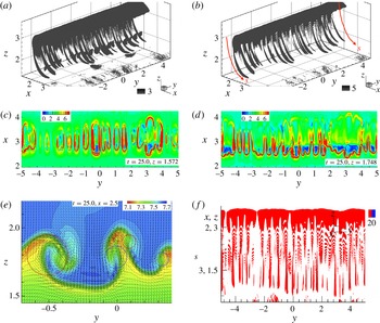
, ranging from approximately 2.16 to 3.04. The larger-scale nature of the RTI structures (which are quasi-2D) is even more starkly illustrated by visualising the second invariant of the instantaneous velocity gradient,
 $Q=-u_{i,j}u_{j,i}/2$
. This common definition of
 $Q$
is one half of the difference between the squared values of the asymmetric (rotation) and symmetric (shear) parts of the velocity gradient tensor, so the criterion
 $Q>0$
corresponds to regions where vorticity dominates strain. Figure 12(a,b) shows this quantity at
 $t=24.5$
and 25. The braid structures are quite elongated (their length greatly exceeds their cross-stream dimensions) and are dominated by strong rotation, so the
 $Q$
field contains large magnitudes of
 $Q$
, which increase rapidly with time. They have, on average, a spanwise wavelength of around one half of the RTI wavelength of
 $0.5h$
(because each one is one half of the counter-rotating vortex pair created at the edges of each RTI mushroom). At
 $t=25$
there is a stagnation point in the velocity field around
 $x=2.2$
,
 $z=2$
(although the precise location depends on spanwise position), which is mirrored by the density field shown in figure 8(b). So, as described above (figure 10), the structures illustrated in figure 12 are stretched both downwards and downstream, and upwards and upstream, which naturally enhances their inherent vorticity. They can eventually be looped at the ends of their extent, but identifying such apparently closed ‘end-loops’ is tricky – it requires close control of the
 $Q$
value and particular view orientations. However, suitably chosen horizontal slices, for example, can show their closed loop form, as illustrated by figure 12(c), which shows vorticity magnitude contours on the
 $z=1.57$
plane at
 $t=25$
. Because this is near the bottom of the cylindrical interface (see figures 8
b and 9), the 3D corrugated nature of the interface appears as a series of closed vorticity loops identifying the high-vorticity regions at the edges of the spanwise-separated RTI structures. Figure 12(d) shows the vorticity magnitude (which is dominated by the streamwise vorticity component) on the rather higher horizontal plane
 $z=1.75$
, where the apparent loops do not close, because of the particular slicing location. (We emphasise that these loops and the apparent rings in figure 12(c) are essentially an artifact of visually slicing the thin, curved and corrugated vorticity (and density) sheet containing the RTI structures, rather than evidence of any independent inherent flow structures.) The vorticity plots also emphasise that the structures merge at some points across the span, leading to larger wavelength contributions to the spectra (see below). Incidentally, one might at first think, looking at figure 12(a) for example, that the braids are of centrifugal origin, given their apparent visual similarity with Görtler vortices. But they both begin and continue in regions of the flow that cannot be susceptible to such centrifugal instabilities, since the circumferential velocity is increasing, rather than decreasing, with increasing distance from the centre of rotation of the local streamlines.
Figure 12(e) is a localised section of a vertical cut through (almost) a couple of the RTI mushrooms at
 $x=2.5$
,
 $t=25$
, showing both density contours and individual velocity vectors, and emphasising the high-vorticity (braid) regions near the lateral interfaces between two adjacent mushrooms – one growing up and the other down. These vorticity roll-ups (identified by the red and blue circles in figure 12
e) are driven by the baroclinic process involving lateral density gradients. The noticeable spread of the inter-core spacing of the roll-ups indicates that the RTI instability is relatively broad-band although with a reasonably well-defined ‘centre’ wavelength that fits well with that suggested by (3.1).
Note particularly the short lateral structures evident in figure 12( f), with a wavevector aligned normal to the underlying RTI structures. Recall that these latter structures are inclined in the
 $x{-}z$
plane, and figure 12( f) is not a
 $y{-}z$
plane cut at a single
 $x$
location, but an assembly of such cuts, showing essentially the (quasi-2D, vortex tube/braid) structures viewed normal to the curved surface whose direction is indicated roughly by the
 $s$
coordinate shown in figure 12(b). The very small secondary structures are most pronounced around
 $y=2.5{-}3.5$
, in the later and more developed region of the RTI structures where their shear layers have been stretched (by RTI between their fingers) to be very thin. In fact, their wavelength clearly decreases with increasing
 $s$
, which is exactly what one would expect for KH structures on a thinning interface. So they can be interpreted as secondary KH instabilities (from spanwise vorticity) and are eventually responsible for breaking down the RTI remnants into turbulence. Interpretive care is needed here, however, as the scales of these secondary motions are not far removed from the grid scale. Zoomed-in views at various orientations did not help to identify their nature with great certainty, and further even more refined computations would be needed to confirm our interpretation. (Very recent computations of the same flow at twice the resolution, however, have confirmed the existence of these KH structures.) One certainly anticipates a possible ‘zoo’ of instabilities once the relatively thin ‘open cylinder’ density sheet has developed, rather like that discussed by Mashayek & Peltier (Reference Mashayek and Peltier2012a
) in the context of stratified shear flow transition. Which instability appears first is strongly dependent not only on the Reynolds number but also on the resolution; it is perhaps only because of the very fine mesh used here that RTI is the first to appear and KH can subsequently be seen. With a coarser mesh, it is entirely possible that RTI would not be seen – being suppressed by numerical diffusion – so that the ‘zoo’ misses its initial instability type. The same could happen for a lower Reynolds number. On the other hand, at a significantly higher
 $\mathit{Re}$
, KH instabilities could perhaps occur before the RTI, because of the much thinner interface.
Note finally that some oval-shaped blobs of concentrated vorticity located periodically along
 $y$
can be seen in figure 12(a). These are slightly above the elongated vortex tubes and roughly inside the pair of tubes that can appear to be looped at the ends. This area (
 $x\approx 3,z\approx 2$
) is actually between two higher-density layers (see figure 11 for
 $x=3.04$
) and probably contains the results of complicated mutual 3D interactions of the RTI mushroom hat tops from the two bent layers that join upstream at
 $2.5\leqslant x\leqslant 2.8$
and
 $z\approx 2$
(figure 8
c).
These various features of the later transition process have not been explicitly seen by previous authors in similar situations, probably because of grid-size limitations. It has been recognised, however, that the formation of smaller-scale instabilities on the RTI structures must be part of the later nonlinear stage breakdown to broad-band turbulence (see e.g. Youngs (Reference Youngs1984), Cook et al. (Reference Cook, Cabot and Miller2004) and Abarzhi (Reference Abarzhi2010), although in these studies the small-scale secondary instabilities were under-resolved so the earlier transition stages were only very approximately captured). Nonetheless, there are clear similarities between our results and some of the features seen in other scenarios. For example, the elongated streaky structures (vortex tubes/braids, on the edges of the RTI mushrooms) that extend along the curved vortex sheet are not dissimilar in appearance to the structures extending along the horizontal vortex sheet in the stratified shear layer examined by Fritts & Garten (Reference Fritts and Garten1996) and later authors. Note, however, that previous authors did not have RTI structures as the precursors to the longitudinal rolls (often because their particular scenarios had large-scale KH billows providing the primary instability).
3.3. The late stages – beyond
$t=22$
; deductions from spectral information

A number of spanwise spectra of the density fluctuations, averaged over the region
 $1.25\leqslant x\leqslant 5$
,
 $1.25\leqslant z\leqslant 3.75$
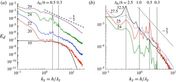
, are shown in figure 13. Most of the transition time scale is covered by the spectra shown in figure 13(a). Clearly, at
 $t=10$
the white-noise seeding is dominant over all but the highest wavenumbers. The high-wavenumber roll-off is caused by diffusional processes weakening energy at the smallest scales of the applied noise. Note that this occurs well before any likely affects of the grid size; the latter is equivalent to
 $k_{y}=50$
(so that the natural aliasing point is at
 $k_{y}=25$
). At significantly higher Reynolds or Prandtl numbers, this diffusional roll-off would occur at higher
 $k_{y}$
but its proper resolution would eventually be hampered by the mesh restrictions.
Non-dimensional spanwise spectra of the density fluctuations,
 $E_{d}=E(\hat{{\it\rho}}^{\prime 2})$
, averaged over the region
 $1.25\leqslant x\leqslant 5$
,
 $1.25\leqslant z\leqslant 3.75$
. The vertical dotted lines denote the wavelengths: (a)
 ${\it\lambda}_{y}=h/k_{y}=0.3h$
and
 $0.5h$
; and (b)
 ${\it\lambda}_{y}=h/k_{y}=0.3h$
,
 $0.5h$
,
 $1.0h$
and
 $2.5h$
. The
 $t$
values are shown by each spectrum.

As time progresses, there is a rapid amplification of the first mode (
 ${\it\lambda}_{y}=10h$
) as noted earlier and, inevitably, adjacent modes. This is evident in the spectrum for
 $t=20$
, for example, which can be compared with figure 4(b), where the effect of the second mode can also be identified (although its amplitude, whilst very significant compared to the noise, is much lower than that of the first mode). Subsequently, a dominant mode with a wavelength around
 $0.5h$
emerges (
 $k_{y}=2$
), as also noted earlier. The value of
 ${\it\lambda}_{y}=0.45h$
for the most dominant mode, suggested by (3.1), can of course only provide a relatively crude estimate, in view of both the uncertainty in the appropriate value of the density difference and the complicated nature of the present case compared to the simple situation yielding (3.1), as discussed earlier. Remnants of a
 ${\it\lambda}_{y}=0.3h$
mode can still be seen at
 $t=24$
, although this mode is actually strongest at much earlier times (between
 $t=10$
and
 $t=15$
). By
 $t\approx 25$
the
 ${\it\lambda}_{y}=0.5h$
mode is at its strongest (compare figure 11), but soon after that the dominance of any particular mode has disappeared, as shown by the spectra in figure 13(b), which are concentrated on the time range
 $24\leqslant t\leqslant 27.5$
and have expanded scales. The peak at
 ${\it\lambda}_{y}=0.3h$
(
 $k_{y}=3.33$
) just evident at
 $t=24$
has disappeared by
 $t=25$
whereas the peak at
 ${\it\lambda}_{y}=0.5h$
(
 $k_{y}=2$
) has grown to a maximum around
 $t=25$
but has disappeared completely by
 $t=27.5$
. So by at least
 $t=29$
the spectrum has a classical turbulence shape with a clear inertial region having a
 $-\frac{5}{3}$
slope, as seen in figure 13(a). Note that in the turbulent patch the density is essentially acting as a passive scalar (the flow is well mixed and density gradients are very weak), so a
 $-\frac{5}{3}$
spectral region is expected for the density as well as velocity fluctuations. It is worth noting here that by
 $t\approx 28.5$
the turbulent kinetic energy and its component Reynolds stresses have all reached their maximum values (as seen in figure 3
a) and fall only marginally to the essentially steady values during the period of the fully developed turbulent patch. One could view the whole transition process as being essentially complete by this time. All signs of individual modes around the original instability wavelengths have disappeared and the overturned patch becomes essentially steady and fully turbulent. This is fully discussed in Yakovenko et al. (Reference Yakovenko, Thomas and Castro2011). Note, however, that after
 $t\approx 24$
a noticeable peak in the spectra is present around
 ${\it\lambda}_{y}=2.5h$
(
 $k_{y}=0.4$
); this grows with time and in fact becomes the dominant peak for quite a long time. Although it slowly subsides (relatively) as energy across all other wave modes increases until transition is complete, it remains visible up to
 $t=45$
at least. It could most naturally be seen as a signature of the size of the entire wave-breaking region and, more interestingly, that of the emerging toroidal vortices (see figure 18). We discuss this further below, but note here that, in their laboratory experiments on a very similar flow, Eiff et al. (Reference Eiff, Huteau and Tolu2005) noted a peak in the spanwise velocity spectrum at almost exactly the same wavelength.
The mushroom structures so clearly seen in figure 11 and discussed in the previous section rapidly begin to merge and break down after
 $t\approx 25$
, not least because of the effect of the smaller-scale KH instabilities, so that visualisations like those in figures 11 and 12 but at later times show only the apparently random nature of genuine turbulence – energy has been spread across all scales, most of which have largely saturated by around
 $t=29$
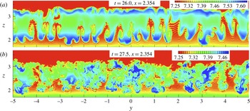
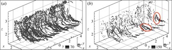
as noted above, removing also the dominance of the first mode. This is shown in figures 14 and 15 where, respectively, density contours and the instantaneous velocity gradient invariant,
 $Q$
, are presented for
 $t=26$
and 27.5. Maximum
 $Q$
values increase rapidly with time, up to approximately 1500 at
 $t=27.5$
, but subsequently relax somewhat by the time the turbulent patch is fully developed (
 $t\approx 35$
), largely because the intense features containing the highest vorticity (the braids) have disappeared. Notice that in figure 15(b) both open and closed vortex loops can be identified; two of them are highlighted by the red ellipses. These are remnants of the loops discussed earlier (and see figure 12
c), but as time progresses the range of scales rapidly increases and, even if the loops remain intact, it becomes more difficult to identify them within the turbulent field.
Density contours at
 $x=2.35$
, for (a)
 $t=26$
and (b)
 $t=27.5$
.

Velocity gradient invariant contours at
 $t=27.5$
, for (a)
 $Q=70$
and (b)
 $Q=150$
. In panel (b), the red ellipses identify the typical U- and O-shaped structures discussed in § 3.2.

We return now to the spanwise mode with
 ${\it\lambda}_{y}\approx 2.5h$
, notable in the spectra at later times and mentioned earlier. Note, incidentally, that it is unlikely that this mode is significantly dependent on the spanwise domain of the computations (
 $10h$
), not least because it was found too in the experiments of Eiff & Bonneton (Reference Eiff and Bonneton2000) and Eiff et al. (Reference Eiff, Huteau and Tolu2005), for which the domain ranged up to
 $32h$
. From one perspective it could be seen as a result of preferential amplification of that mode in the original laminar wave field, effectively adding a small but noticeable spanwise waviness to what would otherwise be a 2D large-scale convective overturning roller. This certainly occurs and in that scenario the spectral peak is not directly related to the RTI mushroom structures, which have much smaller spanwise wavelengths. In particular, at
 $t\approx 24$
, before there is very much evidence of any merging of RTI structures, both wavelengths exist simultaneously (see figure 13). They have magnitudes of similar order. Recall that figure 13 shows spectra averaged over the whole breaking region, so the peak at
 ${\it\lambda}_{y}=2.5$
(
 $k_{y}=0.4$
) is higher than that for the
 ${\it\lambda}_{y}=0.5$
(
 $k_{y}=2$
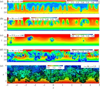
) mode because the latter arises from much more localised structures around the ‘cylindrical’ density interface. However, spanwise slices of the density field at times a little later suggest a merging of the RTI mushroom structures to form larger patches wider apart and thus yielding larger spanwise wavelength. This was noted earlier in the context of figure 12(c,d). It is illustrated further in figure 16, for
 $25\leqslant t\leqslant 27.5$
. The merging is evident around
 $y=-4.5,\ -2.5$
and 3.5 (figure 16
a–c), and this generates a noticeable set of patches that are still visible at
 $t=30$
(figure 16
d). Instantaneous density fields at
 $y=0$
are shown in figure 17 for
 $t=27.5$
and 30; at other spanwise locations the views would be very similar except shifted slightly in
 $x$
because of the underlying spanwise waviness, so vertical slices in the
 $y{-}z$
plane may emphasise the latter. This is evident in figure 16(c) for a slice taken at
 $x=1.96$
. Figure 17(a) shows that this slice is near the front of the turbulent patch; the most developed parts of the overall patch are perhaps those which arise directly from merging structures and at some spanwise locations the patches ‘poke through’ that vertical constant-
 $x$
plane whereas at other spanwise locations they do not. Figure 16(e), which shows a horizontal slice at
 $t=30$
,
 $z=2.5$
, emphasises the point; the upstream extent of the larger structures varies significantly across the span.
(a–d) Spanwise density contours in the
 $y{-}z$
plane at various
 $t,\ x$
values: (a) 25, 2.16; (b) 26, 2.16; (c) 27.5, 1.96; and (d) 30.0, 2.35. (e) Horizontal slice at
 $z=2.5$
(denoted by the dashed line in panel (d)) of the density field at
 $t=30$
.

Density contours at
 $y=0$
, for (a)
 $t=27.5$
and (b)
 $t=30.0$
.

(a,c,d) Instantaneous (‘quasi-’) streamlines at
 $t=32.5$
and (b) total vorticity contours at
 $t=32.5$
,
 $y=-0.2$
: (a) streamwise–vertical plane at
 $y=-0.2$
; (c) spanwise–vertical plane at
 $x=2.74$
; (d) spanwise–streamwise plane at
 $z=2.26$
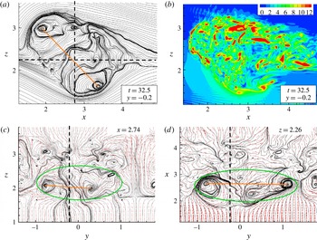
. Panels (c) and (d) also show velocity vectors. The straight dashed lines in panel (a) identify the planes shown in panels (c) and (d); the straight dashed lines in the latter identify the plane shown in panel (a). Imprints of a toroidal structure in each plane are identified by the ellipses in panels (c) and (d), and by lines joining approximate vortex centres.

As noted above, this spanwise
 ${\it\lambda}_{y}\approx 2.5h$
mode has previously been seen in laboratory experiments (Eiff & Bonneton Reference Eiff and Bonneton2000), and also in related numerical studies (Gheusi et al.
Reference Gheusi, Stein and Eiff2000), at low
 $\mathit{Re}\approx 200$
, as well as in the much higher-
 $\mathit{Re}$
experiments of Eiff et al. (Reference Eiff, Huteau and Tolu2005). It was linked with large-scale toroidal vortices identified by those authors, rather than any explicit RTI structure merging or, indeed, any amplification of a wave mode in the original density field. In fact, these authors made no mention of any RTI structures, although Eiff et al. (Reference Eiff, Huteau and Tolu2005) suggested that the initial instability is ‘convectively driven and similar to a Rayleigh–Taylor type instability’. Their toroidal vortices were identified at flow development times late enough for the breaking region to have become almost fully turbulent and were inclined at around 45° in the
 $x{-}z$
plane. Such vortices can also be seen in the present flow. Figure 18 shows three orthogonal planes within the flow at
 $t=32.5$
, i.e. after the entire transitional process is complete. (Recall figure 3
a, which shows that the variances of the fluctuating density and velocities, averaged over the whole breaking region, have reached their steady values and do not change until at least
 $t=55$
(see Yakovenko et al.
Reference Yakovenko, Thomas and Castro2011).) The imprints of a 40°-inclined toroidal vortex having a spanwise scale of approximately
 $2.5h$
are evident in each plane. Three similar structures occur at other locations across the span and, although the flow is fully turbulent, they remain visible at later times and thus seem to be relatively long-lived. They can be associated with the ‘patches’ seen in figure 16(c–e), which should themselves thus be viewed as the incipient precursors to the toroidal vortices. Note that the view seen in figure 18(a) has similarities to the initial twin-vortex pair system seen in figure 8(d), when the flow is still essentially 2D and laminar. During the subsequent transition, the basic gravity wave system remains, and it seems that the combination of the amplification of the initial
 ${\it\lambda}_{y}=2.5h$
mode and the merging of the smaller-scale 3D RTI structures ensures that a toroidal vortex with height around
 $1.5h$
and spanwise scale of
 $2.5h$
is the main emerging structure – hence the spectral peak at that wavelength (figure 13
b), which does not disappear even in the steady flow regime at much later times. It is probably the limited height of the breaking region (
 $1.5h$
) that prevents the development of noticeable 3D structures having a larger spanwise scale (than
 $2.5h$
), at least up to
 $t=45$
. If this is so, then one would not expect this mode to be affected much by changes in Reynolds or Prandtl numbers – it is
 $F_{h}$
that largely determines the size of the breaking region. Eiff & Bonneton (Reference Eiff and Bonneton2000) found that the large-scale toroidal structures were essentially independent of
 $\mathit{Re}$
(for
 $10^{2}\leqslant \mathit{Re}\leqslant 10^{4}$
).
It is worth pointing out that the steady turbulent patch can only remain in place if it possesses a (mean) vorticity distribution characterised by a pair of antiparallel vortex cores, whose joint self-induction velocity (opposing the upstream velocity) enables them to remain stationary with respect to the hill. This pair of vortex structures (i.e. the one identified in figure 9(a,b) and its image in
 $z=0$
) is inherently unstable to small core displacements that lead to lateral wave modes similar to those in, for example, the well-known Crow instability (e.g. Leweke & Williamson Reference Leweke and Williamson1998). Here, it is this instability that perhaps amplifies the earlier
 ${\it\lambda}=2.5h$
wave mode (one of the large-scale components provoked by the topographic forcing). It saturates and, along with the merging of RTI structures, eventually leads to the large toroidal structures.
Note finally that, despite all the above arguments, one should be cautious about interpreting path-line views like those in figure 18 in terms of vortex structures, for instantaneously the vorticity distribution is highly patchy, as seen in figure 18(b), viewed at exactly the same time and spanwise location as figure 18(a).
4. Conclusions
Transition in a convectively breaking internal gravity wave, characterised by a Reynolds number of around 4000 based on the height of the hill generating the wave system and the upstream velocity, has been studied using DNS. It has been conclusively demonstrated that growth of RTI, culminating in their characteristic mushroom-type structures, forms the initial stage of the transition process for this particular breaking-wave case. These quasi-2D structures form along an inclined and bent density interface, which is itself formed by the overturning (essentially spanwise 2D) roller and associated baroclinically generated vorticity, and they produce other vorticity components as they develop. Their spanwise wavelength, first visible above the background noise resulting from the white-noise seeding, depends on the Prandtl number, although our higher
 $\mathit{Pr}$
(LES) results have not been presented here (see below). Grid resolution was sufficient to capture the most amplified modes, whose wavelengths agreed quite well the classical theoretical value for very much simpler cases. Exponential growth in the depth of the mixed region and the variances of the density and velocity fluctuations was found, characteristic of the initial linear phase of the transition in simpler, more classical, two-layer fluid systems widely reported in the literature (e.g. Dalziel et al.
Reference Dalziel, Linden and Youngs1999; Cook et al.
Reference Cook, Cabot and Miller2004). Initial growth of spanwise perturbations was dominated by the largest possible mode in the background wave field – having a wavelength equal to the computational domain width. This mode quickly saturates, and once the mushroom structures appear these dominate and continue to grow, at first without merging.
Unlike classical (two-layer) systems, the velocity field in the present case leads to the mushroom structures being curved in the streamwise–vertical plane as they grow. And as they grow, they naturally lead to a stretching and thinning of the density interface between the vortex tubes (braids) at their edges, creating the conditions for small-scale secondary KH instabilities to develop. Once this has happened, rapid generation of energy across all scales occurs and the broken wave very soon becomes fully turbulent, with the characteristic
 $-\frac{5}{3}$
subrange. There is evidence also of late merging of RTI structures. This, along with the inevitable presence of an amplified
 ${\it\lambda}_{y}=2.5h$
mode of the original wave field, leads to the fully turbulent region having a noticeable, though weak, spectral peak at wavelengths around
 ${\it\lambda}_{y}=2.5h$
. The resultant large-scale long-lived feature emerging from all this is a spanwise sequence of toroidal vortices of that spanwise scale. This has been noted before (e.g. Eiff et al.
Reference Eiff, Huteau and Tolu2005), although the causes were not identified.
It is worth noting that computations at
 $\mathit{Pr}=700$
, using an appropriate subgrid model, revealed a largely similar transition process. It is more rapid, however, and characterised initially by rather smaller-wavelength spanwise structure (because of the sharper density interfaces) than at
 $\mathit{Pr}=1$
. There seems no reason to think that the breakdown to turbulence of atmospheric or oceanic internal waves having the same kind of initial convective overturning structure would differ very much provided the Reynolds number is high enough. The LES studies will be reported elsewhere and an initial summary is given by Yakovenko et al. (Reference Yakovenko, Thomas, Castro and Talamelli2014).
Although we have only studied in detail one specific case here (
 $F_{h}=0.6$
,
 $\mathit{Re}=4000$
), it seems likely that the overall transition scenario would be very similar for other parameter values, provided they yield a breaking lee wave. This requires the Reynolds number to be sufficiently large and, for the present topography, the Froude number to lie roughly in the range
 $0.2<F_{h}<1.0$
(Castro & Snyder Reference Castro and Snyder1993). Of course, other topographic shapes would lead to variations in the critical
 $F_{h}$
range, but these would probably be small and wave breaking certainly requires
 $F_{h}=O(1)$
as a necessary condition. It is also worth emphasising that, although the Reynolds number used is sufficient to yield a fully developed turbulent patch with clear
 $-\frac{5}{3}$
inertial regions in the spectra, it is possible that the route through transition may be somewhat different at significantly higher Reynolds numbers. For example, one might anticipate a rather earlier appearance of the RTI, with subsequently more numerous secondary KH structures and perhaps some evidence of other instability types. Indeed, the C-shaped density and vorticity interface (figures 8 and 9) might, at high enough
 $\mathit{Re}$
, be thin enough for KH instabilities to appear before RTI. The wavelength of the maximum unstable perturbations of the RTI would be smaller according to (3.1) (or, incidentally, larger for higher
 $F_{h}$
). But there is no doubt that the Reynolds number of the present computations is sufficiently high to have yielded evidence of some of the elements of the ‘zoo of instabilities’ discussed by Mashayek & Peltier (Reference Mashayek and Peltier2012b
) in the rather different context of stratified shear flows dominated by large-scale KH billows. There is no completely adequate way of exploring what happens at much higher Reynolds numbers, however, until DNS with very much finer grids becomes computationally feasible (too coarse a grid would simply lead to the earliest fine-scale instabilities being missed), or experimental techniques are developed to allow identification of these instabilities in high-Reynolds-number laboratory experiments. Nonetheless, we believe that the nature of the final fully developed turbulent patch, explored in our earlier paper (Yakovenko et al.
Reference Yakovenko, Thomas and Castro2011), would not be significantly different even at very much higher Reynolds numbers, although the time to full development could well be somewhat shorter and, as noted above, the sequence of transitional instabilities may be different.
Many individual features of the flow computed here have been noted in the literature on atmospheric and oceanic flows, but the present computations have led, we believe, to a more complete description than has been possible before, largely because of their properly DNS nature and a grid adequate to capture transitional details that have not previously been explored for an isolated breaking lee wave. It has been shown that transition in this particular instance is a (relatively unusual) example of a ‘top-down’ process – i.e. starting with the fine-scale (high-frequency) RTI and gradually spreading to larger scales. We close with the observation that the underlying wave field generated by the topography was, in the present cases, essentially 2D. In the field, this will never be the case, and the influence of mean-flow three-dimensionality on the character of the breaking wave and the transition process remains to be explored. It seems unlikely, however, that such effects would remove entirely the basic features that have been identified herein.
Acknowledgements
The work was supported by DSTL and EPSRC (grant number EP/C008561/1), and made use of the Iridis2 and Iridis3 computing resources at the University of Southampton and the HECToR and HPCx facilities at the UK’s national high-performance computing services, provided by EPCC at the University of Edinburgh and by the STFC Daresbury Laboratory. The help of staff at the latter is gratefully acknowledged, as is the UK Turbulence Consortium (EPSRC grant number EP/D044073/1), who kindly supplemented the available computer resources. Support was also received from RFBR (grants 12-01-00050-a and 13-05-00006-a). We are grateful for the substantive and very helpful input from three referees who commented on the first version of this paper.