1 Introduction
Encapsulated bubbles are widely used in various biomedical applications, e.g. as contrast enhancing agents in ultrasound imaging (Lindner Reference Lindner2004) and as carriers in drug delivery systems (Unger et al. Reference Unger, Hersh, Vannan, Matsunaga and McCreery2001). In both cases, controlling the residence time is important. As contrast agents, resonance of bubbles with the applied ultrasound field is not desirable, since it reduces the residence time. As drug delivery carriers, on the other hand, resonance is used for breaking up the bubbles and increasing drug delivery efficiency. Therefore, it is important to understand the dynamics of encapsulated bubbles subject to applied physical forces, and a key set of parameters are their natural frequencies.
In principle, the natural frequencies of encapsulated bubbles are determined by the flow conditions and the mechanical properties of the membrane. The properties of membranes, such as elastic modulus and bending rigidity, can be measured using micropipette aspiration, atomic force microscopy, optical tweezers (Van Vliet, Bao & Suresh Reference Van Vliet, Bao and Suresh2003) or the features of fluid flows (Chang & Olbricht Reference Chang and Olbricht1993a ,Reference Chang and Olbricht b ; Lefebvre et al. Reference Lefebvre, Leclerc, Barthès-Biesel, Walter and Edwards-Lévy2008; Knoche et al. Reference Knoche, Vella, Aumaitre, Degen, Rehage, Cicuta and Kierfeld2013; De Loubens et al. Reference De Loubens, Deschamps, Boedec and Leonetti2015, Reference De Loubens, Deschamps, Edwards-Levy and Leonetti2016). These approaches to measuring membrane properties are applicable to vesicles or capsules, but not to encapsulated bubbles, since the latter tend to burst during experiments. The elastic modulus and viscosity of the coating membranes for bubbles were inferred through observing radial pulsation (De Jong et al. Reference De Jong, Emmer, Van Wamel and Versluis2009; Tu et al. Reference Tu, Guan, Qiu and Matula2009; Segers et al. Reference Segers, de Rond, de Jong, Borden and Versluis2016) and combining constitutive models (Church Reference Church1995; Chatterjee & Sarkar Reference Chatterjee and Sarkar2003; Marmottant et al. Reference Marmottant, van der Meer, Emmer, Versluis, de Jong, Hilgenfeldt and Lohse2005). However, measurements and models based on radial oscillations cannot be extended to shape oscillations directly. The deformation and collapse of the encapsulated bubbles are related to more complicated mechanical characteristics (Stride & Saffari Reference Stride and Saffari2003; Pu, Borden & Longo Reference Pu, Borden and Longo2006). For example, microscopic folds contribute to the stabilization of coated membranes, probably because bending rigidity dominates (Kwan & Borden Reference Kwan and Borden2012).
Ultrasound provides an approach for estimating the natural frequencies of encapsulated bubbles, bypassing specific mechanical parameters and constitutive laws. The main natural frequency can be estimated from resonance in the radial oscillation patterns by modulating the ultrasonic frequency (van der Meer et al. Reference van der Meer, Dollet, Voormolen, Chin, Bouakaz, de Jong, Versluis and Lohse2007). However, knowing the main radial natural frequency is not sufficient, since the natural frequencies of shape modes are crucial for controlling membrane stability. Using ultrasound to estimate the natural frequencies of shape oscillation is non-trivial due to the fact that the shape modes of a bubble are indirectly related to the ultrasound field (induced by parametric instability of the radial oscillation (Plesset & Prosperetti Reference Plesset and Prosperetti1977; Feng & Leal Reference Feng and Leal1997; Brenner, Hilgenfeldt & Lohse Reference Brenner, Hilgenfeldt and Lohse2002)), unlike radial oscillation, which is directly driven by the ultrasound field. Therefore, an alternative approach capable of controlling shape oscillation and estimating natural frequencies of the shape modes directly is needed.
A number of studies have shown that a uniform electric field can be used to induce deformations of gas bubbles (Lee & Kang Reference Lee and Kang1999; Dong et al. Reference Dong, Li, Yu and Yan2006; Spelt & Matar Reference Spelt and Matar2006; Shaw, Spelt & Matar Reference Shaw, Spelt and Matar2009), drops (Taylor Reference Taylor1964; Kang Reference Kang1993; Trinh, Holt & Thiessen Reference Trinh, Holt and Thiessen1996; Dubash & Mestel Reference Dubash and Mestel2007) and vesicles (Kummrow & Helfrich Reference Kummrow and Helfrich1991; Vlahovska et al. Reference Vlahovska, Gracia, Aranda-Espinoza and Dimova2009; Schwalbe, Vlahovska & Miksis Reference Schwalbe, Vlahovska and Miksis2011). Electro-deformation is utilized to measure membrane properties such as viscosity and bending rigidity (Kummrow & Helfrich Reference Kummrow and Helfrich1991; Gracià et al. Reference Gracià, Bezlyepkina, Knorr, Lipowsky and Dimova2010; Salipante & Vlahovska Reference Salipante and Vlahovska2014). In this paper, we show that applying an oscillatory electric field offers another non-invasive way for estimating natural frequencies of shape modes when an encapsulated bubble undergoes oscillations.
Although the dynamics of encapsulated bubbles in an ultrasound field has been widely investigated (Ferrara, Pollard & Borden Reference Ferrara, Pollard and Borden2007; Stride & Coussios Reference Stride and Coussios2010; Lacour et al. Reference Lacour, Guédra, Valier-Brasier and Coulouvrat2018), not much work has been done on the encapsulated bubble in an oscillating electric field, perhaps due to the increased complexity involving bubble dynamics, electrodynamics and membrane mechanics. The ultrasound field could be simply modelled as a pressure wave. By contrast, modelling the dynamics of encapsulated bubbles in an electric field is more complicated. In this paper, we use the Taylor–Melcher leaky dielectric model (Melcher & Taylor Reference Melcher and Taylor1969). This is a classical model proposed in the 1960s for studying the electrohydrodynamics of a gas bubble immersed in poorly conducting liquids where most of the charges exist only at the gas–liquid interface (Saville Reference Saville1997). Accordingly, electrohydrodynamic coupling occurs only at the interface due to electric Maxwell stress. For an encapsulated bubble, the permittivities of gas and membrane are similar and much smaller than that of water. Therefore, the electric interaction of the encapsulated bubble can be well approximated by the leaky dielectric model, which was originally proposed for a gas bubble without a membrane (Lee & Kang Reference Lee and Kang1999; Spelt & Matar Reference Spelt and Matar2006), while the mechanical properties are different for a bubble with and without a membrane. The leaky dielectric model has been validated by several experimental studies (Vizika & Saville Reference Vizika and Saville1992; Tsukada et al. Reference Tsukada, Katayama, Ito and Hozawa1993) and recently derived from the coupled Navier–Stokes–Poisson–Nernst–Planck (NS-PNP) framework (Schnitzer & Yariv Reference Schnitzer and Yariv2015).
The encapsulating membranes for medical application are composed of polymer, albumin, galactose and lipid (Lindner Reference Lindner2004), with varying mechanical properties. Early studies incorporated linear elasticity (Church Reference Church1995), effective surface tension (Marmottant et al. Reference Marmottant, van der Meer, Emmer, Versluis, de Jong, Hilgenfeldt and Lohse2005) and hyperelasticity (Tsiglifis & Pelekasis Reference Tsiglifis and Pelekasis2008) to investigate the dynamical behaviour of a coated bubble. Following Liu et al. (Reference Liu, Sugiyama, Takagi and Matsumoto2011, Reference Liu, Sugiyama, Takagi and Matsumoto2012), we use a general membrane model consistent with the continuum mechanics framework, including the in-plane stress, transverse shear tension and bending moment, proposed by Barthès-Biesel & Rallison (Reference Barthès-Biesel and Rallison1981) and Pozrikidis (Reference Pozrikidis2001), in the current study.
Using Legendre polynomials, we are able to derive a set of differential equations for the radial and shape oscillations under steady and unsteady applied electric fields, which can be solved using a numerical method. The deformed shape agrees well with experimental observations reported in the literature, under a steady electric field. Our results for an incompressible membrane with bending rigidity show that the interfacial charge distribution is determined by the magnitude of the shape modes, as well as the permittivity and conductivity of the external and internal fluids. For a hyperelastic membrane with bending rigidity, our results show that the encapsulated bubble can modulate its oscillating frequency and reach a stable shape oscillation at an appreciable amplitude.
The rest of the paper is organized as follows. In § 2, we derive the mathematical model for the electric field and flow field. These two fields are combined in stress balance at an interface (§ 2.3) and charge transport equation (§ 2.4). In § 3.1, a simplified case for a membrane with bending rigidity only is investigated and the results are compared with the experimental results by Kummrow & Helfrich (Reference Kummrow and Helfrich1991). In § 3.2, the dynamics of a bubble coated by a hyperelastic membrane with bending rigidity is investigated. The feasibility of applying an oscillatory electric field to find out the natural frequency of shape modes is revealed. In § 4, concluding remarks are given.
2 Problem formulation
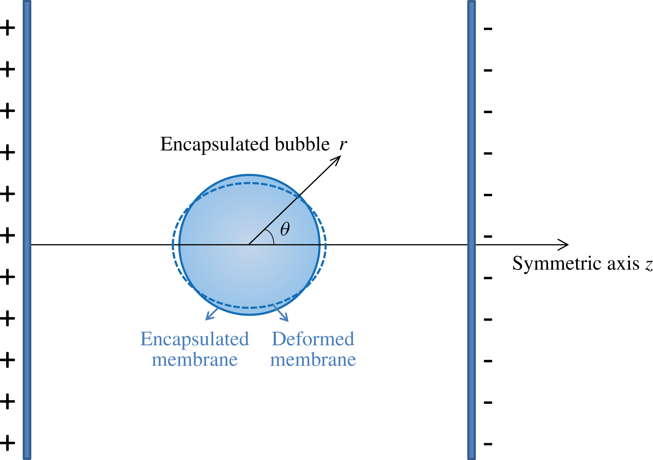
The coordinates of the encapsulated bubble in a spatially uniform electric field.

We consider an encapsulated bubble suspended between two conducting plates parallel to each other. Applying a temporally constant or varying voltage yields a steady or oscillatory electric field. We assume the separation between the two plates is much larger than the bubble radius, so the effect of boundary confinement can be neglected. The flow field and electric field are assumed to be axisymmetric with the axis of symmetry along the direction of the applied electric field
 $z$
and through the centre of the bubble (figure 1). We establish a polar coordinate system with the origin at the centre of the bubble and consider a perturbation to a spherical shape. The positions of the material points at the bubble interface are thereby determined by the radial and zenith directions and expanded in terms of the (associated) Legendre polynomials as
 $$\begin{eqnarray}\displaystyle & \displaystyle r(\unicode[STIX]{x1D703},t)=R(t)+\mathop{\sum }_{k=2}^{\infty }a_{k}(t)P_{k}(\cos \unicode[STIX]{x1D703}), & \displaystyle\end{eqnarray}$$
 $$\begin{eqnarray}\displaystyle & \displaystyle \unicode[STIX]{x1D6E9}(\unicode[STIX]{x1D703},t)=\unicode[STIX]{x1D703}+\frac{1}{R}\mathop{\sum }_{k=1}^{\infty }b_{k}(t)P_{k}^{1}(\cos \unicode[STIX]{x1D703}), & \displaystyle\end{eqnarray}$$
where
 $a_{k}$
is the amplitude of the shape mode and
 $b_{k}$
is the amplitude of the displacements of material points along the zenith direction accompanying the deformation. It is noted that the summation in (2.1) is from
 $k=2$
since the order of
 $k=1$
represents the translation of a bubble without deformation and does not account for shape modes. The summation in (2.2) is from
 $k=1$
in which the first-order mode
 $b_{1}$
denotes the extension or compression along the interface while the shape remains spherical. The surface shape function is defined as
 $$\begin{eqnarray}S\equiv r-R(t)-\mathop{\sum }_{k=2}^{\infty }a_{k}(t)P_{k}(\cos \unicode[STIX]{x1D703})=0,\end{eqnarray}$$
from which the unit normal vector
 $\boldsymbol{n}$
and tangential vector
 $\boldsymbol{t}$
are obtained:
 $$\begin{eqnarray}\displaystyle & \displaystyle \boldsymbol{n}=\frac{\unicode[STIX]{x1D735}S}{|\unicode[STIX]{x1D735}S|}\simeq \boldsymbol{e}_{r}-\boldsymbol{e}_{\unicode[STIX]{x1D703}}\mathop{\sum }_{k=2}^{\infty }\frac{a_{k}}{R}P_{k}^{1}(\cos \unicode[STIX]{x1D703}), & \displaystyle\end{eqnarray}$$
 $$\begin{eqnarray}\displaystyle & \displaystyle \boldsymbol{t}\simeq \boldsymbol{e}_{\unicode[STIX]{x1D703}}+\boldsymbol{e}_{r}\mathop{\sum }_{k=2}^{\infty }\frac{a_{k}}{R}P_{k}^{1}(\cos \unicode[STIX]{x1D703}). & \displaystyle\end{eqnarray}$$
2.1 Electric field
We assume that there is no free charge in the bulk, and it only exists on the bubble interface. According to Gauss’s law and Faraday’s law without induction, the external and internal electric fields
 $\boldsymbol{E}_{ex}$
and
 $\boldsymbol{E}_{in}$
are irrotational and solenoidal. Therefore, the electric fields can be expressed by the electric potentials as
 $$\begin{eqnarray}\boldsymbol{E}_{ex}=-\unicode[STIX]{x1D735}\unicode[STIX]{x1D713}_{ex},\quad \boldsymbol{E}_{in}=-\unicode[STIX]{x1D735}\unicode[STIX]{x1D713}_{in},\end{eqnarray}$$
and the electric potentials
 $\unicode[STIX]{x1D713}_{ex}$
and
 $\unicode[STIX]{x1D713}_{in}$
satisfy the Laplace equations
 $$\begin{eqnarray}\unicode[STIX]{x1D6FB}^{2}\unicode[STIX]{x1D713}_{ex}=0,\quad \unicode[STIX]{x1D6FB}^{2}\unicode[STIX]{x1D713}_{in}=0.\end{eqnarray}$$
The boundary conditions at the bubble interface for the electric potentials are the continuity of the tangential components of the electric fields and the jump condition for the normal components of the electric displacement vectors (Saville Reference Saville1997; Lee & Kang Reference Lee and Kang1999), given respectively by
 $$\begin{eqnarray}\displaystyle & \displaystyle \boldsymbol{t}\boldsymbol{\cdot }\unicode[STIX]{x1D735}\unicode[STIX]{x1D713}_{ex}=\boldsymbol{t}\boldsymbol{\cdot }\unicode[STIX]{x1D735}\unicode[STIX]{x1D713}_{in}, & \displaystyle\end{eqnarray}$$
 $$\begin{eqnarray}\displaystyle & \displaystyle -\unicode[STIX]{x1D700}_{ex}\boldsymbol{n}\boldsymbol{\cdot }\unicode[STIX]{x1D735}\unicode[STIX]{x1D713}_{ex}+\unicode[STIX]{x1D700}_{in}\boldsymbol{n}\boldsymbol{\cdot }\unicode[STIX]{x1D735}\unicode[STIX]{x1D713}_{in}=q/\unicode[STIX]{x1D700}_{0}, & \displaystyle\end{eqnarray}$$
where
 $\unicode[STIX]{x1D700}_{0}$
is the permittivity of vacuum,
 $\unicode[STIX]{x1D700}_{ex}$
and
 $\unicode[STIX]{x1D700}_{in}$
are the relative permittivities of the liquid and gas phases, respectively, and
 $q$
is the interfacial charge density, which is also expanded in terms of the Legendre polynomials:
 $$\begin{eqnarray}q=\mathop{\sum }_{k=0}^{\infty }q_{k}(t)P_{k}(\cos \unicode[STIX]{x1D703}).\end{eqnarray}$$
Owing to the spatially uniform distribution of electric field as
 $r\rightarrow \infty$
and the requirement of regularity at
 $r=0$
, the solutions to the Laplace equations (2.7) have the forms of
 $$\begin{eqnarray}\unicode[STIX]{x1D713}_{ex}(r,\unicode[STIX]{x1D703},t)=-\frac{A_{0}}{r}P_{0}(\cos \unicode[STIX]{x1D703})-\left(E_{0}r+\frac{A_{1}(t)R(t)^{3}}{r^{2}}\right)P_{1}(\cos \unicode[STIX]{x1D703})-\mathop{\sum }_{k=2}^{\infty }\frac{A_{k}(t)}{r^{k+1}}P_{k}(\cos \unicode[STIX]{x1D703}),\end{eqnarray}$$
 $$\begin{eqnarray}\displaystyle \unicode[STIX]{x1D713}_{in}(r,\unicode[STIX]{x1D703},t)=-\mathop{\sum }_{k=0}^{\infty }B_{k}(t)r^{k}P_{k}(\cos \unicode[STIX]{x1D703}), & & \displaystyle\end{eqnarray}$$
where
 $E_{0}$
is the magnitude of the applied electric field, which can be constant or vary with time. It is noted that
 $A_{1}$
is written separately from
 $A_{k}$
(
 $k\geqslant 2$
) in (2.11). The reason is that we want to make
 $A_{1}$
and
 $E_{0}$
the same dimension for convenience, and we will find in the following that the terms with the first-order Legendre polynomials
 $P_{1}(\cos \unicode[STIX]{x1D703})$
are dominant in the electric field.
Substituting (2.11) and (2.12) into (2.8) and (2.9), and making use of the orthogonality of the Legendre polynomials, we obtain
 $A_{0}=0$
. Coefficient
 $B_{0}$
is a constant related to the electric potential jump across the interface. We will see below that this constant does not affect the electric stress at the interface, as it depends on the electric field, which is proportional to the potential gradient. From the above boundary conditions,
 $q_{0}$
is obtained to be zero. The solutions to
 $q_{k}$
(
 $k\geqslant 1$
) will be given in § 2.4. The other coefficients
 $A_{1}$
,
 $B_{1}$
,
 $A_{2}$
,
 $B_{2}$
,
 $A_{k}$
and
 $B_{k}$
(
 $k\geqslant 3$
) are obtained as
 $$\begin{eqnarray}\displaystyle & \displaystyle A_{1}=\frac{E_{0}(\unicode[STIX]{x1D700}_{ex}-\unicode[STIX]{x1D700}_{in})-q_{1}/\unicode[STIX]{x1D700}_{0}}{2\unicode[STIX]{x1D700}_{ex}+\unicode[STIX]{x1D700}_{in}}-\frac{6a_{2}}{5R}\frac{(\unicode[STIX]{x1D700}_{ex}+2\unicode[STIX]{x1D700}_{in})q_{1}/\unicode[STIX]{x1D700}_{0}+E_{0}(\unicode[STIX]{x1D700}_{ex}-\unicode[STIX]{x1D700}_{in})^{2}}{(2\unicode[STIX]{x1D700}_{ex}+\unicode[STIX]{x1D700}_{in})^{2}}, & \displaystyle\end{eqnarray}$$
 $$\begin{eqnarray}\displaystyle & \displaystyle B_{1}=\frac{3\unicode[STIX]{x1D700}_{ex}E_{0}-q_{1}/\unicode[STIX]{x1D700}_{0}}{2\unicode[STIX]{x1D700}_{ex}+\unicode[STIX]{x1D700}_{in}}-\frac{6a_{2}}{5R}\frac{(-q_{1}/\unicode[STIX]{x1D700}_{0}+3\unicode[STIX]{x1D700}_{ex}E_{0})(\unicode[STIX]{x1D700}_{ex}-\unicode[STIX]{x1D700}_{in})}{(2\unicode[STIX]{x1D700}_{ex}+\unicode[STIX]{x1D700}_{in})^{2}}, & \displaystyle\end{eqnarray}$$
 $$\begin{eqnarray}\displaystyle & \displaystyle A_{2}=-\frac{R^{4}q_{2}}{\unicode[STIX]{x1D700}_{0}(3\unicode[STIX]{x1D700}_{ex}+2\unicode[STIX]{x1D700}_{in})}-\frac{6a_{3}R^{3}}{7}\frac{3E_{0}(\unicode[STIX]{x1D700}_{ex}-\unicode[STIX]{x1D700}_{in})^{2}+(\unicode[STIX]{x1D700}_{ex}+5\unicode[STIX]{x1D700}_{in})q_{1}/\unicode[STIX]{x1D700}_{0}}{(2\unicode[STIX]{x1D700}_{ex}+\unicode[STIX]{x1D700}_{in})(3\unicode[STIX]{x1D700}_{ex}+2\unicode[STIX]{x1D700}_{in})}, & \displaystyle\end{eqnarray}$$
 $$\begin{eqnarray}\displaystyle & \displaystyle B_{2}=-\frac{q_{2}}{R\unicode[STIX]{x1D700}_{0}(3\unicode[STIX]{x1D700}_{ex}+2\unicode[STIX]{x1D700}_{in})}-\frac{3a_{3}}{7R^{2}}\frac{15E_{0}\unicode[STIX]{x1D700}_{ex}(\unicode[STIX]{x1D700}_{ex}-\unicode[STIX]{x1D700}_{in})+(-7\unicode[STIX]{x1D700}_{ex}+4\unicode[STIX]{x1D700}_{in})q_{1}/\unicode[STIX]{x1D700}_{0}}{(2\unicode[STIX]{x1D700}_{ex}+\unicode[STIX]{x1D700}_{in})(3\unicode[STIX]{x1D700}_{ex}+2\unicode[STIX]{x1D700}_{in})}, & \displaystyle\end{eqnarray}$$
 $$\begin{eqnarray}\displaystyle A_{k} & = & \displaystyle -\frac{R^{k+2}q_{k}/\unicode[STIX]{x1D700}_{0}}{(k+1)\unicode[STIX]{x1D700}_{ex}+k\unicode[STIX]{x1D700}_{in}}+\frac{R^{k+1}}{2\unicode[STIX]{x1D700}_{ex}+\unicode[STIX]{x1D700}_{in}}\nonumber\\ \displaystyle & & \displaystyle \times \,\left\{\frac{k}{2k-1}a_{k-1}\left[3E_{0}(\unicode[STIX]{x1D700}_{ex}-\unicode[STIX]{x1D700}_{in})-\frac{q_{1}}{\unicode[STIX]{x1D700}_{0}}\frac{(k+5)\unicode[STIX]{x1D700}_{ex}+(2k+1)\unicode[STIX]{x1D700}_{in}}{(k+1)\unicode[STIX]{x1D700}_{ex}+k\unicode[STIX]{x1D700}_{in}}\right]\right.\nonumber\\ \displaystyle & & \displaystyle -\left.\frac{k+1}{2k+3}a_{k+1}\left[\frac{3kE_{0}(\unicode[STIX]{x1D700}_{ex}-\unicode[STIX]{x1D700}_{in})^{2}}{(k+1)\unicode[STIX]{x1D700}_{ex}+k\unicode[STIX]{x1D700}_{in}}+\frac{q_{1}}{\unicode[STIX]{x1D700}_{0}}\frac{(4-k)\unicode[STIX]{x1D700}_{ex}+(4k+2)\unicode[STIX]{x1D700}_{in}}{(k+1)\unicode[STIX]{x1D700}_{ex}+k\unicode[STIX]{x1D700}_{in}}\right]\!\right\}\!,\end{eqnarray}$$
 $$\begin{eqnarray}\displaystyle \hspace{-25.00003pt}B_{k} & = & \displaystyle -\frac{R^{-k+1}q_{k}/\unicode[STIX]{x1D700}_{0}}{(k+1)\unicode[STIX]{x1D700}_{ex}+k\unicode[STIX]{x1D700}_{in}}+\frac{R^{-k}}{(k+1)\unicode[STIX]{x1D700}_{ex}+k\unicode[STIX]{x1D700}_{in}}\left\{\frac{k(k-1)}{2k-1}a_{k-1}\frac{q_{1}}{\unicode[STIX]{x1D700}_{0}}\right.\nonumber\\ \displaystyle & & \displaystyle -\left.\frac{k+1}{2k+3}a_{k+1}\left[\frac{3(2k+1)E_{0}\unicode[STIX]{x1D700}_{ex}(\unicode[STIX]{x1D700}_{ex}-\unicode[STIX]{x1D700}_{in})}{2\unicode[STIX]{x1D700}_{ex}+\unicode[STIX]{x1D700}_{in}}+\frac{q_{1}}{\unicode[STIX]{x1D700}_{0}}\frac{(1-4k)\unicode[STIX]{x1D700}_{ex}+(k+2)\unicode[STIX]{x1D700}_{in}}{2\unicode[STIX]{x1D700}_{ex}+\unicode[STIX]{x1D700}_{in}}\right]\!\right\}\!.\qquad\end{eqnarray}$$
The details of applying Legendre polynomials to the boundary conditions (2.8) and (2.9) are given in appendices A and B.
2.2 Flow field
We assume that the flow field inside the bubble is negligible and consider only the flow field outside the bubble by the incompressible Navier–Stokes equations:
 $$\begin{eqnarray}\displaystyle & \displaystyle \unicode[STIX]{x1D735}\boldsymbol{\cdot }\boldsymbol{u}=0, & \displaystyle\end{eqnarray}$$
 $$\begin{eqnarray}\displaystyle & \displaystyle \unicode[STIX]{x1D70C}\frac{\unicode[STIX]{x2202}\boldsymbol{u}}{\unicode[STIX]{x2202}t}+\unicode[STIX]{x1D70C}[(\boldsymbol{u}-w\boldsymbol{e}_{z})\boldsymbol{\cdot }\unicode[STIX]{x1D735}]\boldsymbol{u}=-\unicode[STIX]{x1D735}p+\unicode[STIX]{x1D707}\unicode[STIX]{x1D735}\boldsymbol{\cdot }(\unicode[STIX]{x1D735}\boldsymbol{u}+\unicode[STIX]{x1D735}\boldsymbol{u}^{\text{T}}), & \displaystyle\end{eqnarray}$$
where
 $\boldsymbol{u}$
and
 $p$
are the velocity and pressure, respectively,
 $w$
is the translational velocity of the bubble along the
 $z$
axis, and
 $\unicode[STIX]{x1D70C}$
and
 $\unicode[STIX]{x1D707}$
are the liquid density and viscosity, respectively. The velocity and pressure are decomposed into a potential part (with subscript
 $p$
) and viscous pressure correction (with subscript
 $v$
) as (Prosperetti Reference Prosperetti1977)
 $$\begin{eqnarray}\boldsymbol{u}=\boldsymbol{u}_{p}+\boldsymbol{u}_{v},\quad p=p_{p}+p_{v}.\end{eqnarray}$$
The potential part is obtained by the velocity potential
 $\unicode[STIX]{x1D711}$
, which satisfies the Laplace equation and the boundary condition:
 $$\begin{eqnarray}\frac{\unicode[STIX]{x2202}S}{\unicode[STIX]{x2202}t}+(\unicode[STIX]{x1D735}\unicode[STIX]{x1D711}-w\boldsymbol{e}_{z})\boldsymbol{\cdot }\unicode[STIX]{x1D735}S=0,\end{eqnarray}$$
where
 $S$
is the surface function defined in (2.3). The velocity potential is obtained therefrom as
 $$\begin{eqnarray}\unicode[STIX]{x1D711}=\mathop{\sum }_{k=0}^{\infty }\frac{C_{k}(t)}{r^{k+1}}P_{k}(\cos \unicode[STIX]{x1D703}),\end{eqnarray}$$
where
 $$\begin{eqnarray}\displaystyle & \displaystyle C_{0}=-{\dot{R}}R^{2}, & \displaystyle\end{eqnarray}$$
 $$\begin{eqnarray}\displaystyle & \displaystyle C_{1}=-\frac{R^{3}}{2}w+\frac{3}{10}R^{2}wa_{2}, & \displaystyle\end{eqnarray}$$
 $$\begin{eqnarray}\displaystyle & \displaystyle C_{k}=-\frac{R^{k+2}}{k+1}\left({\dot{a}}_{k}+\frac{2{\dot{R}}a_{k}}{R}\right)+\frac{3k}{2}R^{k+1}w\left(\frac{a_{k+1}}{2k+3}-\frac{a_{k-1}}{2k-1}\right)\!. & \displaystyle\end{eqnarray}$$
The velocity of the potential part is obtained consequently as
 $$\begin{eqnarray}\boldsymbol{u}_{p}=\frac{\unicode[STIX]{x2202}\unicode[STIX]{x1D711}}{\unicode[STIX]{x2202}r}\boldsymbol{e}_{r}+\frac{1}{r}\frac{\unicode[STIX]{x2202}\unicode[STIX]{x1D711}}{\unicode[STIX]{x2202}\unicode[STIX]{x1D703}}\boldsymbol{e}_{\unicode[STIX]{x1D703}},\end{eqnarray}$$
and the pressure of the potential part is obtained by the Bernoulli equation as
 $$\begin{eqnarray}p_{p}=p_{\infty }-\unicode[STIX]{x1D70C}\left[\frac{\unicode[STIX]{x2202}\unicode[STIX]{x1D711}}{\unicode[STIX]{x2202}t}+\frac{1}{2}|\unicode[STIX]{x1D735}\unicode[STIX]{x1D711}|^{2}-w\boldsymbol{e}_{z}\boldsymbol{\cdot }\unicode[STIX]{x1D735}\unicode[STIX]{x1D711}\right]\!.\end{eqnarray}$$
The viscous correction part is solved by the toroidal component of the vorticity
 $T_{k}(r,t)$
, which satisfies the linearized Navier–Stokes equation (Prosperetti Reference Prosperetti1977)
 $$\begin{eqnarray}\unicode[STIX]{x1D70C}\frac{\unicode[STIX]{x2202}T_{k}}{\unicode[STIX]{x2202}t}+\unicode[STIX]{x1D70C}\frac{\unicode[STIX]{x2202}}{\unicode[STIX]{x2202}r}[{\dot{R}}(R/r)^{2}T_{k}]-\unicode[STIX]{x1D707}\frac{\unicode[STIX]{x2202}^{2}T_{k}}{\unicode[STIX]{x2202}r^{2}}+\unicode[STIX]{x1D707}k(k+1)r^{-2}T_{k}=0.\end{eqnarray}$$
The velocity and pressure are written in terms of the toroidal field as
 $$\begin{eqnarray}\displaystyle & \displaystyle \boldsymbol{u}_{v}=\left(\mathop{\sum }_{k=1}^{\infty }T_{k}(r,t)P_{k}(\cos \unicode[STIX]{x1D703})-\frac{\unicode[STIX]{x2202}\unicode[STIX]{x1D6F7}}{\unicode[STIX]{x2202}r}\right)\boldsymbol{e}_{r}-\frac{1}{r}\frac{\unicode[STIX]{x2202}\unicode[STIX]{x1D6F7}}{\unicode[STIX]{x2202}\unicode[STIX]{x1D703}}\boldsymbol{e}_{\unicode[STIX]{x1D703}}, & \displaystyle\end{eqnarray}$$
 $$\begin{eqnarray}\displaystyle & \displaystyle p_{v}=\mathop{\sum }_{k=1}^{\infty }k\left\{\unicode[STIX]{x1D707}_{l}T_{k}(R,t)/R+\unicode[STIX]{x1D70C}({\dot{R}}/R_{i})\int _{R}^{\infty }[(R/s)^{3}-1](R/s)^{k}T_{k}(s,t)\,\text{d}s\right\}P_{k}(\cos \unicode[STIX]{x1D703}),\hspace{-5.0pt} & \displaystyle \nonumber\\ \displaystyle & & \displaystyle\end{eqnarray}$$
where
 $$\begin{eqnarray}\displaystyle \unicode[STIX]{x1D6F7} & = & \displaystyle \mathop{\sum }_{k=1}^{\infty }P_{k}(\cos \unicode[STIX]{x1D703})\left[\left(-\frac{k+1}{2k+1}\int _{R}^{\infty }s^{-k}T_{k}(s,t)\,\text{d}s+\frac{k+1}{2k+1}\int _{R}^{r}s^{-k}T_{k}(s,t)\,\text{d}s\right)r^{k}\right.\nonumber\\ \displaystyle & & \displaystyle +\left.\left(-\frac{k}{2k+1}R^{2k+1}\int _{R}^{\infty }s^{-k}T_{k}(s,t)\,\text{d}s+\frac{k}{2k+1}\int _{R}^{r}s^{k+1}T_{k}(s,t)\,\text{d}s\right)r^{-(k+1)}\right]\!.\nonumber\\ \displaystyle & & \displaystyle\end{eqnarray}$$
The partial differential equation (2.29) will be solved numerically subject to the boundary conditions to be discussed. The velocity
 $\boldsymbol{u}_{v}$
and pressure
 $p_{v}$
are subsequently obtained. The detailed derivation for the flow field can be found in Liu et al. (Reference Liu, Sugiyama, Takagi and Matsumoto2012) and Liu, Sugiyama & Takagi (Reference Liu, Sugiyama and Takagi2016).
2.3 Stress balance at the interface
The stress balance at the interface includes the pressure difference, the jump of the viscous and Maxwell stresses, and the membrane stress (for encapsulated bubbles only) or surface tension (for gas bubbles only), in the normal and tangential directions, respectively:
 $$\begin{eqnarray}\displaystyle & \displaystyle -p_{ex}+\boldsymbol{n}\boldsymbol{\cdot }\unicode[STIX]{x1D64F}_{ex}\boldsymbol{\cdot }\boldsymbol{n}+\boldsymbol{n}\boldsymbol{\cdot }\unicode[STIX]{x1D648}_{ex}\boldsymbol{\cdot }\boldsymbol{n}=-p_{in}+\boldsymbol{n}\boldsymbol{\cdot }\unicode[STIX]{x1D648}_{in}\boldsymbol{\cdot }\boldsymbol{n}+F_{n}, & \displaystyle\end{eqnarray}$$
 $$\begin{eqnarray}\displaystyle & \displaystyle \boldsymbol{n}\boldsymbol{\cdot }\unicode[STIX]{x1D64F}_{ex}\boldsymbol{\cdot }\boldsymbol{t}+\boldsymbol{n}\boldsymbol{\cdot }\unicode[STIX]{x1D648}_{ex}\boldsymbol{\cdot }\boldsymbol{t}=\boldsymbol{n}\boldsymbol{\cdot }\unicode[STIX]{x1D648}_{in}\boldsymbol{\cdot }\boldsymbol{t}+F_{t}, & \displaystyle\end{eqnarray}$$
where
 $p_{ex}$
and
 $p_{in}$
are the pressure outside and inside the bubble, respectively;
 $\unicode[STIX]{x1D64F}_{ex}$
is the viscous stress tensor at the liquid side, while the viscous stress in the bubble is neglected due to the small viscosity of gas;
 $\unicode[STIX]{x1D648}_{ex}$
and
 $\unicode[STIX]{x1D648}_{in}$
are the Maxwell stress tensors outside and inside the bubble, respectively; and
 $F_{n}$
and
 $F_{t}$
are the normal and tangential interfacial stresses, respectively. The derivations of these terms are given in detail as follows.
The external pressure
 $p_{ex}$
is calculated by (2.21b
), (2.28) and (2.31), and evaluated at the bubble interface. The interior of the bubble is gas, which is compressible. The internal pressure
 $p_{in}$
is considered to be uniformly distributed, calculated by
 $$\begin{eqnarray}p_{in}=p_{in0}\left(\frac{V_{0}}{V}\right)^{\unicode[STIX]{x1D6E4}},\end{eqnarray}$$
where
 $V$
is the volume of the bubble, and the subscript 0 indicates the initial value;
 $\unicode[STIX]{x1D6E4}$
is the polytropic index.
The viscous stress tensor at the liquid side
 $\unicode[STIX]{x1D64F}_{ex}$
is expressed as
 $$\begin{eqnarray}\unicode[STIX]{x1D64F}_{ex}=\unicode[STIX]{x1D707}(\unicode[STIX]{x1D735}\boldsymbol{u}+\unicode[STIX]{x1D735}\boldsymbol{u}^{\text{T}}),\end{eqnarray}$$
where the velocity includes the potential part and viscous correction, given by (2.21a ), (2.27) and (2.30). The normal and tangential components of the viscous stress are written explicitly as
 $$\begin{eqnarray}\displaystyle \boldsymbol{n}\boldsymbol{\cdot }\unicode[STIX]{x1D64F}_{ex}\boldsymbol{\cdot }\boldsymbol{n} & = & \displaystyle P_{0}2\unicode[STIX]{x1D707}\left[-\frac{2{\dot{R}}}{R}\right]+P_{1}2\unicode[STIX]{x1D707}\left[-\frac{3w}{R}+\frac{27}{5}\frac{w}{R^{2}}a_{2}+\frac{2}{R}\int _{R}^{\infty }s^{-1}T_{1}(s,t)\,\text{d}s\right]\nonumber\\ \displaystyle & & \displaystyle +\,\mathop{\sum }_{k=2}^{\infty }P_{k}2\unicode[STIX]{x1D707}\left\{-(k+2)\frac{{\dot{a}}_{k}}{R}-2(k-1)\frac{{\dot{R}}}{R^{2}}a_{k}\right.\nonumber\\ \displaystyle & & \displaystyle +\,\frac{w}{R^{2}}\left[-\frac{3k(k-1)(k+4)}{2(2k-1)}a_{k-1}+\frac{3(k+1)(k^{2}+2k+6)}{2(2k+3)}a_{k+1}\right]\nonumber\\ \displaystyle & & \displaystyle +\left.k(k+1)R^{k-2}\int _{R}^{\infty }s^{-k}T_{k}(s,t)\,\text{d}s\right\}\!,\end{eqnarray}$$
 $$\begin{eqnarray}\displaystyle \boldsymbol{n}\boldsymbol{\cdot }\unicode[STIX]{x1D64F}_{ex}\boldsymbol{\cdot }\boldsymbol{t} & = & \displaystyle P_{1}^{1}2\unicode[STIX]{x1D707}\left[\frac{3w}{2R}-\frac{9wa_{2}}{10R^{2}}-\frac{T_{1}(R,t)}{2R}-\frac{1}{R}\int _{R}^{\infty }s^{-1}T_{1}(s,t)\,\text{d}s\right]\nonumber\\ \displaystyle & & \displaystyle +\,\mathop{\sum }_{k=2}^{\infty }P_{k}^{1}2\unicode[STIX]{x1D707}\left[\frac{k+2}{k+1}\frac{{\dot{a}}_{k}}{R}+\frac{1-k}{k+1}\frac{{\dot{R}}a_{k}}{R^{2}}+\frac{3k(k+2)}{2}\frac{w}{R^{2}}\left(\frac{a_{k-1}}{2k-1}-\frac{a_{k+1}}{2k+3}\right)\right.\nonumber\\ \displaystyle & & \displaystyle -\left.\frac{T_{k}(R,t)}{2R}-R^{k-2}\int _{R}^{\infty }s^{-k}T_{k}(s,t)\,\text{d}s\right]\!.\end{eqnarray}$$
The Maxwell stress tensor in the liquid
 $\unicode[STIX]{x1D648}_{ex}$
is given by the electric field as (Landau, Lifshitz & Pitaevskii Reference Landau, Lifshitz and Pitaevskii1984)
 $$\begin{eqnarray}\unicode[STIX]{x1D648}_{ex}=\unicode[STIX]{x1D700}_{ex}\unicode[STIX]{x1D700}_{0}(\boldsymbol{E}_{ex}\boldsymbol{E}_{ex}-{\textstyle \frac{1}{2}}|\boldsymbol{E}_{ex}|^{2}\boldsymbol{I}).\end{eqnarray}$$
Written in terms of the electric potential by using (2.6), the normal and tangential components of the Maxwell stress (2.39) become
 $$\begin{eqnarray}\displaystyle & \displaystyle \boldsymbol{n}\boldsymbol{\cdot }\unicode[STIX]{x1D648}_{ex}\boldsymbol{\cdot }\boldsymbol{n}=\unicode[STIX]{x1D700}_{ex}\unicode[STIX]{x1D700}_{0}\left\{\frac{1}{2}\left[\left(\frac{\unicode[STIX]{x2202}\unicode[STIX]{x1D713}_{ex}}{\unicode[STIX]{x2202}r}\right)^{2}-\left(\frac{1}{r}\frac{\unicode[STIX]{x2202}\unicode[STIX]{x1D713}_{ex}}{\unicode[STIX]{x2202}\unicode[STIX]{x1D703}}\right)^{2}\right]-\frac{2}{r^{2}}\frac{\unicode[STIX]{x2202}\unicode[STIX]{x1D713}_{ex}}{\unicode[STIX]{x2202}r}\frac{\unicode[STIX]{x2202}\unicode[STIX]{x1D713}_{ex}}{\unicode[STIX]{x2202}\unicode[STIX]{x1D703}}\mathop{\sum }_{k=2}^{\infty }a_{k}P_{k}^{1}\right\}\!,\quad & \displaystyle\end{eqnarray}$$
 $$\begin{eqnarray}\displaystyle & \displaystyle \boldsymbol{n}\boldsymbol{\cdot }\unicode[STIX]{x1D648}_{ex}\boldsymbol{\cdot }\boldsymbol{t}=\unicode[STIX]{x1D700}_{ex}\unicode[STIX]{x1D700}_{0}\left\{\frac{1}{r}\frac{\unicode[STIX]{x2202}\unicode[STIX]{x1D713}_{ex}}{\unicode[STIX]{x2202}r}\frac{\unicode[STIX]{x2202}\unicode[STIX]{x1D713}_{ex}}{\unicode[STIX]{x2202}\unicode[STIX]{x1D703}}+\frac{1}{r}\left[\left(\frac{\unicode[STIX]{x2202}\unicode[STIX]{x1D713}_{ex}}{\unicode[STIX]{x2202}r}\right)^{2}-\left(\frac{1}{r}\frac{\unicode[STIX]{x2202}\unicode[STIX]{x1D713}_{ex}}{\unicode[STIX]{x2202}\unicode[STIX]{x1D703}}\right)^{2}\right]\mathop{\sum }_{k=2}^{\infty }a_{k}P_{k}^{1}\right\}\!.\quad & \displaystyle\end{eqnarray}$$
Substituting in the expressions of electric potential (2.11), and the relations of the Legendre polynomials in appendix A, the components of the Maxwell stress at the liquid side of the interface are written explicitly as
 $$\begin{eqnarray}\displaystyle \boldsymbol{n}\boldsymbol{\cdot }\unicode[STIX]{x1D648}_{ex}\boldsymbol{\cdot }\boldsymbol{n} & = & \displaystyle \unicode[STIX]{x1D700}_{ex}\unicode[STIX]{x1D700}_{0}\left\{\frac{1}{2}(E_{0}-2A_{1})^{2}P_{1}^{2}-\frac{1}{2}(E_{0}+A_{1})^{2}\left(\frac{\text{d}P_{1}}{\text{d}\unicode[STIX]{x1D703}}\right)^{2}\right.\nonumber\\ \displaystyle & & \displaystyle +\,\mathop{\sum }_{k=2}^{\infty }\left[\frac{6A_{1}}{R}(E_{0}-2A_{1})a_{k}P_{1}^{2}P_{k}-\frac{k+1}{R^{k+2}}(E_{0}-2A_{1})A_{k}P_{1}P_{k}\right.\nonumber\\ \displaystyle & & \displaystyle +\,\frac{3A_{1}}{R}a_{k}(E_{0}+A_{1})P_{k}\left(\frac{\text{d}P_{1}}{\text{d}\unicode[STIX]{x1D703}}\right)^{2}-\frac{A_{k}}{R^{k+2}}(E_{0}+A_{1})\frac{\text{d}P_{1}}{\text{d}\unicode[STIX]{x1D703}}\frac{\text{d}P_{k}}{\text{d}\unicode[STIX]{x1D703}}\nonumber\\ \displaystyle & & \displaystyle \left.\left.-\,\frac{2}{R}(E_{0}-2A_{1})(E_{0}+A_{1})a_{k}P_{1}\frac{\text{d}P_{1}}{\text{d}\unicode[STIX]{x1D703}}\frac{\text{d}P_{k}}{\text{d}\unicode[STIX]{x1D703}}\right]\right\}\nonumber\\ \displaystyle & = & \displaystyle P_{0}\unicode[STIX]{x1D700}_{ex}\unicode[STIX]{x1D700}_{0}\left\{\frac{1}{6}(2A_{1}^{2}-8E_{0}A_{1}-E_{0}^{2})-\frac{4}{5}E_{0}(E_{0}-2A_{1})\frac{a_{2}}{R}\right\}\nonumber\\ \displaystyle & & \displaystyle +\,P_{1}\unicode[STIX]{x1D700}_{ex}\unicode[STIX]{x1D700}_{0}\left\{-(2E_{0}-A_{1})\frac{6A_{2}}{5R^{4}}\right\}\nonumber\\ \displaystyle & & \displaystyle +\,P_{2}\unicode[STIX]{x1D700}_{ex}\unicode[STIX]{x1D700}_{0}\left\{\frac{1}{3}(5A_{1}^{2}-2A_{1}E_{0}+2E_{0}^{2})+(A_{1}-2E_{0})\frac{12A_{3}}{7R^{5}}\right.\nonumber\\ \displaystyle & & \displaystyle +\left.\frac{2a_{2}}{7R}(-11A_{1}^{2}+20A_{1}E_{0}-2E_{0}^{2})\right\}\nonumber\\ \displaystyle & & \displaystyle +\,\mathop{\sum }_{k=3}^{\infty }P_{k}\unicode[STIX]{x1D700}_{ex}\unicode[STIX]{x1D700}_{0}\left\{(A_{1}-2E_{0})\frac{(k+1)(k+2)}{(2k+3)R^{k+3}}A_{k+1}+[A_{1}(3k-1)-E_{0}]\right.\nonumber\\ \displaystyle & & \displaystyle \times \,\frac{kA_{k-1}}{(2k-1)R^{k+1}}+ [A_{1}^{2}(-6k^{2}-6k+3)+A_{1}E_{0}(11k^{2}+11k-6)\nonumber\\ \displaystyle & & \displaystyle -\,E_{0}^{2}k(k+1)\!]\frac{2}{(2k-1)(2k+3)}\frac{a_{k}}{R}+(2A_{1}-E_{0})[kA_{1}+(k+3)E_{0}]\nonumber\\ \displaystyle & & \displaystyle \times \,\frac{2(k+1)(k+2)}{(2k+3)(2k+5)}\frac{a_{k+2}}{R}-(2A_{1}-E_{0})[(k+1)A_{1}+(k-2)E_{0}]\nonumber\\ \displaystyle & & \displaystyle \times \,\left.\frac{2k(k-1)}{(2k-3)(2k-1)}\frac{a_{k-2}}{R}\right\}\!,\end{eqnarray}$$
 $$\begin{eqnarray}\displaystyle \boldsymbol{n}\boldsymbol{\cdot }\unicode[STIX]{x1D648}_{ex}\boldsymbol{\cdot }\boldsymbol{t}=\mathop{\sum }_{k=2}^{\infty }\unicode[STIX]{x1D700}_{ex}\unicode[STIX]{x1D700}_{0}\left[\frac{1}{3}(2A_{1}^{2}-8A_{1}E_{0}-E_{0}^{2})\frac{a_{k}}{R}\right]P_{k}^{1}(\cos \unicode[STIX]{x1D703}). & & \displaystyle\end{eqnarray}$$
The Maxwell stress in the bubble is calculated in a similar way as (2.39), (2.40) and (2.41) with the subscript replaced by ‘in’. By substituting (2.6), and (2.12), the normal and tangential components of the Maxwell stress at the gas side of the interface are written as
 $$\begin{eqnarray}\displaystyle \boldsymbol{n}\boldsymbol{\cdot }\unicode[STIX]{x1D648}_{in}\boldsymbol{\cdot }\boldsymbol{n} & = & \displaystyle \unicode[STIX]{x1D700}_{in}\unicode[STIX]{x1D700}_{0}\left\{\frac{1}{2}B_{1}^{2}P_{1}^{2}-\frac{1}{2}B_{1}^{2}\left(\frac{\text{d}P_{1}}{\text{d}\unicode[STIX]{x1D703}}\right)^{2}\right.\nonumber\\ \displaystyle & & \displaystyle +\left.\mathop{\sum }_{k=2}^{\infty }\left[B_{1}B_{k}kR^{k-1}P_{1}P_{k}-B_{1}B_{k}R^{k-1}\frac{\text{d}P_{1}}{\text{d}\unicode[STIX]{x1D703}}\frac{\text{d}P_{k}}{\text{d}\unicode[STIX]{x1D703}}-\frac{2B_{1}^{2}}{R}a_{k}P_{1}\frac{\text{d}P_{1}}{\text{d}\unicode[STIX]{x1D703}}\frac{\text{d}P_{k}}{\text{d}\unicode[STIX]{x1D703}}\right]\right\}\nonumber\\ \displaystyle & = & \displaystyle P_{0}\unicode[STIX]{x1D700}_{in}\unicode[STIX]{x1D700}_{0}\left[-\frac{1}{6}B_{1}^{2}-\frac{4}{5}B_{1}^{2}\frac{a_{2}}{R}\right]+P_{1}\unicode[STIX]{x1D700}_{in}\unicode[STIX]{x1D700}_{0}\left[-\frac{2}{5}RB_{1}B_{2}\right]\nonumber\\ \displaystyle & & \displaystyle +\,P_{2}\unicode[STIX]{x1D700}_{in}\unicode[STIX]{x1D700}_{0}\left[\frac{2}{3}B_{1}^{2}-\frac{3}{7}R^{2}B_{1}B_{3}-\frac{4}{7R}B_{1}^{2}a_{2}\right]\nonumber\\ \displaystyle & & \displaystyle +\,\mathop{\sum }_{k=3}^{\infty }P_{k}\unicode[STIX]{x1D700}_{in}\unicode[STIX]{x1D700}_{0}\left[-\frac{k+1}{2k+3}B_{1}B_{k+1}R^{k}+\frac{2k(k-1)}{2k-1}B_{1}B_{k-1}R^{k-2}\right.\nonumber\\ \displaystyle & & \displaystyle -\,\frac{2k(k+1)}{(2k-1)(2k+3)}B_{1}^{2}\frac{a_{k}}{R}-\frac{2(k+1)(k+2)(k+3)}{(2k+3)(2k+5)}B_{1}^{2}\frac{a_{k+2}}{R}\nonumber\\ \displaystyle & & \displaystyle +\left.\frac{2k(k-1)(k-2)}{(2k-3)(2k-1)}B_{1}^{2}\frac{a_{k-2}}{R}\right]\!,\end{eqnarray}$$
 $$\begin{eqnarray}\displaystyle \boldsymbol{n}\boldsymbol{\cdot }\unicode[STIX]{x1D648}_{in}\boldsymbol{\cdot }\boldsymbol{t}=\mathop{\sum }_{k=2}^{\infty }\unicode[STIX]{x1D700}_{in}\unicode[STIX]{x1D700}_{0}\left[-\frac{1}{3}B_{1}^{2}\frac{a_{k}}{R}\right]P_{k}^{1}(\cos \unicode[STIX]{x1D703}). & & \displaystyle\end{eqnarray}$$
In the general case, the membrane stress
 $\boldsymbol{F}$
includes the in-plane stress and bending moment (Green & Adkins Reference Green and Adkins1960)
 $$\begin{eqnarray}\boldsymbol{F}=-(\boldsymbol{P}\boldsymbol{\cdot }\unicode[STIX]{x1D735})\boldsymbol{\cdot }(\unicode[STIX]{x1D749}+\unicode[STIX]{x1D64C}\boldsymbol{n}),\end{eqnarray}$$
where
 $\boldsymbol{P}~(=\boldsymbol{I}-\boldsymbol{n}\boldsymbol{n})$
is the tangential projection operator,
 $\unicode[STIX]{x1D749}~(=\unicode[STIX]{x1D70F}_{\unicode[STIX]{x1D703}}\boldsymbol{e}_{\unicode[STIX]{x1D703}}\boldsymbol{e}_{\unicode[STIX]{x1D703}}+\unicode[STIX]{x1D70F}_{\unicode[STIX]{x1D719}}\boldsymbol{e}_{\unicode[STIX]{x1D719}}\boldsymbol{e}_{\unicode[STIX]{x1D719}})$
is the in-plane stress and
 $\unicode[STIX]{x1D64C}$
is the transverse shear tension, associated with the bending moment
 $\boldsymbol{m}~(=m_{\unicode[STIX]{x1D703}}\boldsymbol{e}_{\unicode[STIX]{x1D703}}\boldsymbol{e}_{\unicode[STIX]{x1D703}}+m_{\unicode[STIX]{x1D719}}\boldsymbol{e}_{\unicode[STIX]{x1D719}}\boldsymbol{e}_{\unicode[STIX]{x1D719}})$
as
 $$\begin{eqnarray}\unicode[STIX]{x1D64C}=[(\boldsymbol{P}\boldsymbol{\cdot }\unicode[STIX]{x1D735})\boldsymbol{\cdot }\boldsymbol{m}]\boldsymbol{\cdot }\boldsymbol{P}.\end{eqnarray}$$
For a hyperelastic membrane, we adopt the strain energy function
 $W_{s}$
to connect the in-plane stress
 $\unicode[STIX]{x1D70F}_{i}$
and strain
 $\unicode[STIX]{x1D706}_{i}$
, and the bending energy function
 $W_{b}$
to connect the bending moment
 $m_{i}$
and the bending strain
 $K_{i}$
:
 $$\begin{eqnarray}\displaystyle & \displaystyle \unicode[STIX]{x1D70F}_{i}=\frac{\unicode[STIX]{x1D706}_{i}}{\unicode[STIX]{x1D706}_{\unicode[STIX]{x1D703}}\unicode[STIX]{x1D706}_{\unicode[STIX]{x1D719}}}\frac{\unicode[STIX]{x2202}W_{s}(\unicode[STIX]{x1D706}_{\unicode[STIX]{x1D703}},\unicode[STIX]{x1D706}_{\unicode[STIX]{x1D719}})}{\unicode[STIX]{x2202}\unicode[STIX]{x1D706}_{i}}, & \displaystyle\end{eqnarray}$$
 $$\begin{eqnarray}\displaystyle & \displaystyle m_{i}=\frac{\unicode[STIX]{x1D706}_{i}}{\unicode[STIX]{x1D706}_{\unicode[STIX]{x1D703}}\unicode[STIX]{x1D706}_{\unicode[STIX]{x1D719}}}\frac{\unicode[STIX]{x2202}W_{b}(K_{\unicode[STIX]{x1D703}},K_{\unicode[STIX]{x1D719}})}{\unicode[STIX]{x2202}K_{i}}, & \displaystyle\end{eqnarray}$$
where
 $i$
is chosen as
 $\unicode[STIX]{x1D703}$
and
 $\unicode[STIX]{x1D719}$
alternatively to represent the two principal directions. Bending strain
 $K_{i}$
is defined as
 $$\begin{eqnarray}K_{i}=\unicode[STIX]{x1D706}_{i}\unicode[STIX]{x1D705}_{i}-\unicode[STIX]{x1D705}_{i}^{R}\end{eqnarray}$$
to consider the effect of in-plane strain on the bending moment, where
 $\unicode[STIX]{x1D705}_{i}$
is the principal curvature, calculated by the curvature tensor
 $\unicode[STIX]{x1D63D}=\boldsymbol{P}\boldsymbol{\cdot }\unicode[STIX]{x1D735}\boldsymbol{n}$
to be
 $$\begin{eqnarray}\displaystyle & \displaystyle \unicode[STIX]{x1D705}_{\unicode[STIX]{x1D703}}=\frac{1}{R}-\mathop{\sum }_{k=2}^{\infty }\frac{a_{k}}{R^{2}}\left(P_{k}+\frac{\text{d}^{2}P_{k}}{\text{d}\unicode[STIX]{x1D703}^{2}}\right)\!, & \displaystyle\end{eqnarray}$$
 $$\begin{eqnarray}\displaystyle & \displaystyle \unicode[STIX]{x1D705}_{\unicode[STIX]{x1D719}}=\frac{1}{R}-\mathop{\sum }_{k=2}^{\infty }\frac{a_{k}}{R^{2}}\left(P_{k}+\frac{\cos \unicode[STIX]{x1D703}}{\sin \unicode[STIX]{x1D703}}P_{k}^{1}\right)\!. & \displaystyle\end{eqnarray}$$
As an example, we adopt the neo-Hookean law, a simple form of the strain-softening Mooney–Rivlin law (Mooney Reference Mooney1940), of which the strain energy function is given by
 $$\begin{eqnarray}W_{s}=\frac{G_{s}}{2}\left(\unicode[STIX]{x1D706}_{\unicode[STIX]{x1D703}}^{2}+\unicode[STIX]{x1D706}_{\unicode[STIX]{x1D719}}^{2}+\frac{1}{\unicode[STIX]{x1D706}_{\unicode[STIX]{x1D703}}^{2}\unicode[STIX]{x1D706}_{\unicode[STIX]{x1D719}}^{2}}-3\right)\!,\end{eqnarray}$$
where
 $G_{s}$
is the surface modulus of elasticity. The bending strain energy function is given by the Love law (Love Reference Love1888)
 $$\begin{eqnarray}W_{b}=\frac{G_{b}}{2}(K_{\unicode[STIX]{x1D703}}^{2}+2\unicode[STIX]{x1D710}K_{\unicode[STIX]{x1D703}}K_{\unicode[STIX]{x1D719}}+K_{\unicode[STIX]{x1D719}}^{2}),\end{eqnarray}$$
where
 $G_{b}$
is the bending modulus and
 $\unicode[STIX]{x1D710}$
the Poisson ratio.
Accordingly, the normal and tangential components of the membrane stress are (Liu et al. Reference Liu, Sugiyama and Takagi2016)
 $$\begin{eqnarray}\displaystyle F_{n} & = & \displaystyle \frac{2G_{s}(R^{6}-R_{0}^{6})}{R^{7}}+\left[-12G_{s}\frac{R_{0}^{6}}{R^{8}}b_{1}-2(1+\unicode[STIX]{x1D710})G_{b}\frac{b_{1}}{R^{4}}\right]P_{1}(\cos \unicode[STIX]{x1D703})\nonumber\\ \displaystyle & & \displaystyle +\,\mathop{\sum }_{k=2}^{\infty }\left\{-\frac{G_{s}}{R^{8}}[2(R^{6}-7R_{0}^{6})a_{k}+6k(k+1)R_{0}^{6}b_{k}]\right.\nonumber\\ \displaystyle & & \displaystyle +\left.\frac{G_{b}}{R^{4}}[k(k+1)(k^{2}+k-1+\unicode[STIX]{x1D710})(a_{k}-b_{k})]\right\}P_{k}(\cos \unicode[STIX]{x1D703}),\end{eqnarray}$$
 $$\begin{eqnarray}\displaystyle F_{t} & = & \displaystyle \left[6G_{s}\frac{R_{0}^{6}}{R^{8}}b_{1}+(1+\unicode[STIX]{x1D710})\frac{G_{b}}{R^{4}}b_{1}\right]P_{1}^{1}(\cos \unicode[STIX]{x1D703})\nonumber\\ \displaystyle & & \displaystyle +\,\mathop{\sum }_{k=2}^{\infty }\left\{\frac{G_{s}}{R^{8}}[(R^{6}-7R_{0}^{6})a_{k}+(3k(k+1)R_{0}^{6}+(k-1)(k+2)R^{6})b_{k}]\right.\nonumber\\ \displaystyle & & \displaystyle -\left.\frac{G_{b}}{R^{4}}(k^{2}+k-1+\unicode[STIX]{x1D710})(a_{k}-b_{k})\right\}P_{k}^{1}(\cos \unicode[STIX]{x1D703}).\end{eqnarray}$$
The expressions for the interfacial stresses
 $F_{n}$
and
 $F_{t}$
can be specified depending on constitutive laws for different types of interface. In the following part of this section we keep this notation in the equations and only add superscripts to denote the expansion at specific order of the Legendre polynomials.
We substitute (2.35)–(2.38) and (2.42)–(2.45) into (2.33) and (2.34) and expand them with respect to the Legendre polynomials. Utilizing the orthogonality of the polynomials, we obtain dynamic equations at different orders. The zeroth order of (2.33) provides the dynamics of radial oscillation:
 $$\begin{eqnarray}\displaystyle & & \displaystyle R\ddot{R}+\frac{3}{2}{\dot{R}}^{2}+\frac{1}{\unicode[STIX]{x1D70C}}\left(p_{\infty }-p_{in}+4\unicode[STIX]{x1D707}_{l}\frac{{\dot{R}}}{R}\right)-\frac{1}{4}w^{2}-\frac{1}{\unicode[STIX]{x1D70C}}\unicode[STIX]{x1D700}_{in}\unicode[STIX]{x1D700}_{0}B_{1}^{2}\left(\frac{1}{6}+\frac{4a_{2}}{5R}\right)\nonumber\\ \displaystyle & & \displaystyle \quad -\,\frac{1}{\unicode[STIX]{x1D70C}}\unicode[STIX]{x1D700}_{ex}\unicode[STIX]{x1D700}_{0}\left[\frac{1}{6}(2A_{1}^{2}-8E_{0}A_{1}-E_{0}^{2})-\frac{4}{5}E_{0}(E_{0}-2A_{1})\frac{a_{2}}{R}\right]+\frac{F_{n}^{0}}{\unicode[STIX]{x1D70C}}=0,\end{eqnarray}$$
which is a Rayleigh–Plesset type equation with translational motion and interfacial stresses. We note that the Maxwell stress, as a driving force, is quadratic in electric field strength
 $E_{0}$
, shown by substituting the expressions of
 $A_{1}$
(2.13) and
 $B_{1}$
(2.14) into (2.57). This implies that the oscillatory frequency of the radial mode is twice the frequency of the oscillatory electric field.
The coefficients before the first-order Legendre polynomials
 $P_{1}(\cos \unicode[STIX]{x1D703})$
in (2.33) provide the translational equation:
 $$\begin{eqnarray}\displaystyle & & \displaystyle \frac{1}{2}R{\dot{w}}+\frac{3}{2}{\dot{R}}w-\frac{7}{10}{\dot{w}}a_{2}-\frac{9}{10}w{\dot{a}}_{2}-\frac{6}{5}\frac{{\dot{R}}}{R}wa_{2}\nonumber\\ \displaystyle & & \displaystyle \quad +\,\frac{\unicode[STIX]{x1D707}_{l}T_{1}(R,t)}{\unicode[STIX]{x1D70C}R}+\frac{{\dot{R}}}{R}\int _{R}^{\infty }\left[\left(\frac{R}{s}\right)^{3}-1\right]\left(\frac{R}{s}\right)T_{1}(s,t)\,\text{d}s\nonumber\\ \displaystyle & & \displaystyle \quad +\,\frac{2\unicode[STIX]{x1D707}_{l}}{\unicode[STIX]{x1D70C}}\left(\frac{3w}{R}-\frac{27}{5}\frac{a_{2}}{R^{2}}w-\frac{2}{R}\int _{R}^{\infty }s^{-1}T_{1}(s,t)\,\text{d}s\right)\nonumber\\ \displaystyle & & \displaystyle \quad -\,\frac{2}{5\unicode[STIX]{x1D70C}}\unicode[STIX]{x1D700}_{in}\unicode[STIX]{x1D700}_{0}RB_{1}B_{2}+\frac{1}{\unicode[STIX]{x1D70C}}\unicode[STIX]{x1D700}_{ex}\unicode[STIX]{x1D700}_{0}(2E_{0}-A_{1})\frac{6A_{2}}{5R^{4}}+\frac{F_{n}^{1}}{\unicode[STIX]{x1D70C}}=0,\end{eqnarray}$$
where the first two terms are associated with the inertia of added mass, and the terms of the second and third lines are the drag due to viscosity. The translational motion is induced by the applied electric field. From the first two terms in the last line, we know that the Maxwell stress at this order is proportional to the coefficients
 $A_{2}$
and
 $B_{2}$
. By investigating the expressions (2.15) and (2.16), if the even-order charge distribution and odd-order shape mode are not triggered, which will be demonstrated below, the driving force of the electric field on the translational motion is zero, i.e. the bubble does not translate under a spatially uniform electric field.
The equations of the second-order shape oscillation and the
 $k$
th-order shape oscillation (
 $k\geqslant 3$
) are
 $$\begin{eqnarray}\displaystyle & & \displaystyle \frac{1}{3}R\ddot{a}_{2}+{\dot{R}}{\dot{a}}_{2}+\left(-\frac{1}{3}\ddot{R}-\frac{183}{70}\frac{w^{2}}{R}\right)a_{2}+\frac{3}{4}w^{2}-\frac{15}{14}w{\dot{a}}_{3}-a_{3}\left(\frac{9}{7}\frac{{\dot{R}}}{R}w+\frac{6}{7}{\dot{w}}\right)\nonumber\\ \displaystyle & & \displaystyle \quad +\,\frac{2\unicode[STIX]{x1D707}_{l}T_{2}(R,t)}{\unicode[STIX]{x1D70C}R}+\frac{2{\dot{R}}}{R}\int _{R}^{\infty }\left[\left(\frac{R}{s}\right)^{3}-1\right]\left(\frac{R}{s}\right)^{2}T_{2}(s,t)\,\text{d}s\nonumber\\ \displaystyle & & \displaystyle \quad +\,\frac{2\unicode[STIX]{x1D707}_{l}}{\unicode[STIX]{x1D70C}}\left[4\frac{{\dot{a}}_{2}}{R}+\frac{2{\dot{R}}}{R^{2}}a_{2}-\frac{9a_{3}}{R^{2}}w-6\int _{R}^{\infty }s^{-2}T_{2}(s,t)\,\text{d}s\right]\nonumber\\ \displaystyle & & \displaystyle \quad +\,\frac{1}{\unicode[STIX]{x1D70C}}\unicode[STIX]{x1D700}_{in}\unicode[STIX]{x1D700}_{0}\left(\frac{2}{3}B_{1}^{2}-\frac{3}{7}R^{2}B_{1}B_{3}-\frac{4}{7R}B_{1}^{2}a_{2}\right)\nonumber\\ \displaystyle & & \displaystyle \quad -\,\frac{1}{\unicode[STIX]{x1D70C}}\unicode[STIX]{x1D700}_{ex}\unicode[STIX]{x1D700}_{0}\left[\frac{1}{3}(5A_{1}^{2}-2A_{1}E_{0}+2E_{0}^{2})+(A_{1}-2E_{0})\frac{12A_{3}}{7R^{5}}\right.\nonumber\\ \displaystyle & & \displaystyle \quad +\left.\frac{2a_{2}}{7R}(-11A_{1}^{2}+20A_{1}E_{0}-2E_{0}^{2})\right]+\frac{F_{n}^{2}}{\unicode[STIX]{x1D70C}}=0,\end{eqnarray}$$
 $$\begin{eqnarray}\displaystyle & & \displaystyle \frac{1}{k+1}R\ddot{a}_{k}+\left[\frac{3{\dot{R}}}{k+1}+\frac{2(k+2)\unicode[STIX]{x1D707}_{l}}{\unicode[STIX]{x1D70C}R}\right]{\dot{a}}_{k}\nonumber\\ \displaystyle & & \displaystyle \quad +\,\left[-\frac{k-1}{k+1}\ddot{R}+\frac{4(k-1)\unicode[STIX]{x1D707}_{l}}{\unicode[STIX]{x1D70C}}\frac{{\dot{R}}}{R^{2}}-\frac{9(2k^{4}+3k^{3}+k^{2}+k-1)}{2(2k-1)(2k+1)(2k+3)}\frac{w^{2}}{R}\right]a_{k}\nonumber\\ \displaystyle & & \displaystyle \quad +\,{\dot{a}}_{k-1}\frac{3}{2}w+a_{k-1}\left[\frac{3(k-1){\dot{R}}w}{(2k-1)R}+\frac{k}{2(2k-1)}{\dot{w}}\right]-{\dot{a}}_{k+1}\frac{3(2k+1)}{2(2k+3)}w\nonumber\\ \displaystyle & & \displaystyle \quad -\,a_{k+1}\left[\frac{3(k+1)w{\dot{R}}}{(2k+3)R}+\frac{5k+2}{2(2k+3)}{\dot{w}}\right]\nonumber\\ \displaystyle & & \displaystyle \quad +\,\frac{k\unicode[STIX]{x1D707}_{l}T_{k}(R,t)}{\unicode[STIX]{x1D70C}R}+k\frac{{\dot{R}}}{R}\int _{R}^{\infty }\left[\left(\frac{R}{s}\right)^{3}-1\right]\left(\frac{R}{s}\right)^{k}T_{k}(s,t)\,\text{d}s\nonumber\\ \displaystyle & & \displaystyle \quad +\,\frac{2\unicode[STIX]{x1D707}_{l}}{\unicode[STIX]{x1D70C}}\left\{\frac{w}{R^{2}}\left[\frac{3k(k-1)(k+4)}{2(2k-1)}a_{k-1}-\frac{3(k+1)(k^{2}+2k+6)}{2(2k+3)}a_{k+1}\right]\right.\nonumber\\ \displaystyle & & \displaystyle \quad -\left.k(k+1)R^{k-2}\int _{R}^{\infty }s^{-k}T_{k}(s,t)\,\text{d}s\right\}\nonumber\\ \displaystyle & & \displaystyle \quad +\,\frac{1}{\unicode[STIX]{x1D70C}}\unicode[STIX]{x1D700}_{in}\unicode[STIX]{x1D700}_{0}\left[-\frac{k+1}{2k+3}B_{1}B_{k+1}R^{k}+\frac{2k(k-1)}{2k-1}B_{1}B_{k-1}R^{k-2}-\frac{2k(k+1)}{(2k-1)(2k+3)}\frac{B_{1}^{2}}{R}a_{k}\right.\nonumber\\ \displaystyle & & \displaystyle \quad -\left.\frac{2(k+1)(k+2)(k+3)}{(2k+3)(2k+5)}B_{1}^{2}\frac{a_{k+2}}{R}+\frac{2k(k-1)(k-2)}{(2k-3)(2k-1)}B_{1}^{2}\frac{a_{k-2}}{R}\right]\nonumber\\ \displaystyle & & \displaystyle \quad -\,\frac{1}{\unicode[STIX]{x1D70C}}\unicode[STIX]{x1D700}_{ex}\unicode[STIX]{x1D700}_{0}\left\{(A_{1}-2E_{0})\frac{(k+1)(k+2)}{(2k+3)R^{k+3}}A_{k+1}+[A_{1}(3k-1)-E_{0}]\frac{kA_{k-1}}{(2k-1)R^{k+1}}\right.\nonumber\\ \displaystyle & & \displaystyle \quad +\,[A_{1}^{2}(-6k^{2}-6k+3)+A_{1}E_{0}(11k^{2}+11k-6)-E_{0}^{2}k(k+1)]\frac{2}{(2k-1)(2k+3)}\frac{a_{k}}{R}\nonumber\\ \displaystyle & & \displaystyle \quad +\,(2A_{1}-E_{0})[kA_{1}+(k+3)E_{0}]\frac{2(k+2)(k+2)}{(2k+3)(2k+5)}\frac{a_{k+2}}{R}\nonumber\\ \displaystyle & & \displaystyle \quad +\left.(2A_{1}-E_{0})[(k+1)A_{1}+(k-2)E_{0}]\frac{2k(k-1)}{(2k-3)(2k-1)}\frac{a_{k-2}}{R}\right\}+\frac{F_{n}^{k}}{\unicode[STIX]{x1D70C}}=0.\end{eqnarray}$$
The equation for the second-order shape mode is written separately since the shape oscillation equation is related to the adjacent shape modes, and the lower-order shape mode to the
 $k=2$
mode is the translational motion, denoted by its velocity. In addition, the following results will show that the second-order shape mode is dominant under an electric field.
To solve the toroidal field (2.29) numerically, a boundary condition at the bubble interface is needed. Here we use the tangential stress balance (2.34) and write it in terms of different modes as
 $$\begin{eqnarray}\displaystyle 2\unicode[STIX]{x1D707}\left[\frac{3w}{2R}-\frac{9wa_{2}}{10R^{2}}-\frac{T_{1}(R,t)}{2R}-\frac{1}{R}\int _{R}^{\infty }s^{-1}T_{1}(s,t)\,\text{d}s\right]=F_{t}^{1} & & \displaystyle\end{eqnarray}$$
for
 $k=1$
, and as
 $$\begin{eqnarray}\displaystyle & & \displaystyle 2\unicode[STIX]{x1D707}\left[\frac{k+2}{k+1}\frac{{\dot{a}}_{k}}{R}+\frac{1-k}{k+1}\frac{{\dot{R}}a_{k}}{R^{2}}+\frac{3k(k+2)}{2}\frac{w}{R^{2}}\left(\frac{a_{k-1}}{2k-1}-\frac{a_{k+1}}{2k+3}\right)\right.\nonumber\\ \displaystyle & & \displaystyle \quad -\left.\frac{T_{k}(R,t)}{2R}-R^{k-2}\int _{R}^{\infty }s^{-k}T_{k}(s,t)\,\text{d}s\right]+\,\unicode[STIX]{x1D700}_{ex}\unicode[STIX]{x1D700}_{0}\left[\frac{1}{3}(2A_{1}^{2}-8A_{1}E_{0}-E_{0}^{2})\frac{a_{k}}{R}\right]\nonumber\\ \displaystyle & & \displaystyle \quad +\,\unicode[STIX]{x1D700}_{in}\unicode[STIX]{x1D700}_{0}\left[\frac{1}{3}B_{1}^{2}\frac{a_{k}}{R}\right]=F_{t}^{k}\end{eqnarray}$$
for
 $k\geqslant 2$
.
For a bubble encapsulated with a hyperelastic membrane, the material points at the surface move along the tangential direction as well as the normal direction during deformation. Therefore, the tangential displacement (2.2) should be solved. To completely determine the system of equations, a no-slip condition at the interface, i.e. the continuity of the tangential velocity, is applied (Liu et al. Reference Liu, Sugiyama and Takagi2016)
 $$\begin{eqnarray}-\frac{1}{k+1}{\dot{a}}_{k}-\frac{2{\dot{R}}a_{k}}{(k+1)R}-\frac{3k}{2R}w\left(\!\frac{a_{k-1}}{2k-1}-\frac{a_{k+1}}{2k+3}\!\right)+R_{i}^{k-1}\!\int _{R}^{\infty }\!s^{-k}T_{k}(s,t)\,\text{d}s={\dot{b}}_{k}-\frac{{\dot{R}}b_{k}}{R}.\end{eqnarray}$$
So far, the dynamic equations for the radial oscillation, translation and shape oscillation have been derived and will be solved by using the fourth-order Runge–Kutta method with the static initial condition. The distribution of free charge
 $q_{k}$
at the interface, which is embedded in
 $A_{k}$
and
 $B_{k}$
(2.13)–(2.18), will be solved in the next section.
2.4 Free charge on the interface
In this section, we consider the transport of free charge on the interface caused by the jump of current across the interface and the stretching of the interface. The conservation of charge, written in the integral form, is
 $$\begin{eqnarray}\displaystyle \int _{S(t)}(\unicode[STIX]{x1D705}_{ex}\boldsymbol{n}\boldsymbol{\cdot }\unicode[STIX]{x1D735}\unicode[STIX]{x1D713}_{ex}-\unicode[STIX]{x1D705}_{in}\boldsymbol{n}\boldsymbol{\cdot }\unicode[STIX]{x1D735}\unicode[STIX]{x1D713}_{in})\,\text{d}S=\frac{\text{d}}{\text{d}t}\int _{S(t)}q\,\text{d}S, & & \displaystyle\end{eqnarray}$$
where
 $\unicode[STIX]{x1D705}_{ex}$
and
 $\unicode[STIX]{x1D705}_{in}$
are the conductivity of the liquid and gas phase. It is noted that (2.64) is established based on the local coordinate with origin at the centre of the bubble. Therefore we use the relative velocity
 $$\begin{eqnarray}\bar{\boldsymbol{u}}=\boldsymbol{u}-w\boldsymbol{e}_{z}\end{eqnarray}$$
in the following to establish the dynamic equation for the charge distribution based on a frame of reference moving with the bubble centre.
The area of the interface may be changed under an electric field. Therefore, the time derivative of the area should be considered as shown on the right-hand side of (2.64) or written explicitly as
 $$\begin{eqnarray}\displaystyle \frac{\text{d}}{\text{d}t}\int _{S(t)}q\,\text{d}S=\int _{S(t)}\left(\frac{\text{d}q}{\text{d}t}\,\text{d}S+q\frac{\text{d}}{\text{d}t}\,\text{d}S\right)\!, & & \displaystyle\end{eqnarray}$$
where the second term on the right-hand side is treated using Batchelor’s method (Batchelor Reference Batchelor2000) to calculate the time derivative of a material surface element with vector area
 $\text{d}\boldsymbol{S}$
:
 $$\begin{eqnarray}\displaystyle \frac{\text{d}}{\text{d}t}\,\text{d}\boldsymbol{S}=\text{d}\boldsymbol{S}\,\unicode[STIX]{x1D735}\boldsymbol{\cdot }\bar{\boldsymbol{u}}-(\unicode[STIX]{x1D735}\bar{\boldsymbol{u}})\boldsymbol{\cdot }\text{d}\boldsymbol{S}. & & \displaystyle\end{eqnarray}$$
Writing
 $\text{d}\boldsymbol{S}=\boldsymbol{n}\,\text{d}S$
and taking the inner product of
 $\boldsymbol{n}$
to the above equation yields (Stone Reference Stone1990)
 $$\begin{eqnarray}\displaystyle \frac{\text{d}}{\text{d}t}\,\text{d}S=\text{d}S\,\unicode[STIX]{x1D735}_{s}\boldsymbol{\cdot }\bar{\boldsymbol{u}}. & & \displaystyle\end{eqnarray}$$
Since the material surface element
 $S(t)$
is arbitrary, the integrals of (2.64) can be eliminated,
 $$\begin{eqnarray}\unicode[STIX]{x1D705}_{ex}\boldsymbol{n}\boldsymbol{\cdot }\unicode[STIX]{x1D735}\unicode[STIX]{x1D713}_{ex}-\unicode[STIX]{x1D705}_{in}\boldsymbol{n}\boldsymbol{\cdot }\unicode[STIX]{x1D735}\unicode[STIX]{x1D713}_{in}=\frac{\text{d}q}{\text{d}t}+q\unicode[STIX]{x1D735}_{s}\boldsymbol{\cdot }\bar{\boldsymbol{u}}.\end{eqnarray}$$
The Lagrangian derivative to the charge density is written as
 $$\begin{eqnarray}\frac{\text{d}q}{\text{d}t}=\frac{\unicode[STIX]{x2202}\widetilde{q}}{\unicode[STIX]{x2202}t}+(\bar{\boldsymbol{u}}\boldsymbol{\cdot }\unicode[STIX]{x1D735})\widetilde{q},\end{eqnarray}$$
where
 $q$
should be extended to the neighbourhood of the interface, denoted by
 $\widetilde{q}$
, in order to calculate the derivative (Pereira et al.
Reference Pereira, Trevelyan, Thiele and Kalliadasis2007), as the charge only exists on the interface.
Decomposing
 $\bar{\boldsymbol{u}}$
into the tangential and normal components,
 $$\begin{eqnarray}\displaystyle \bar{\boldsymbol{u}}=\bar{\boldsymbol{u}}_{s}+\bar{\boldsymbol{u}}_{n}=\bar{\boldsymbol{u}}_{s}+(\bar{\boldsymbol{u}}\boldsymbol{\cdot }\boldsymbol{n})\boldsymbol{n}, & & \displaystyle\end{eqnarray}$$
the right-hand side of (2.69) can be written as
 $$\begin{eqnarray}\displaystyle \frac{\text{d}q}{\text{d}t}+q\unicode[STIX]{x1D735}_{s}\boldsymbol{\cdot }\bar{\boldsymbol{u}}=\frac{\unicode[STIX]{x2202}q}{\unicode[STIX]{x2202}t}+\bar{\boldsymbol{u}}_{n}\boldsymbol{\cdot }\boldsymbol{e}_{\unicode[STIX]{x1D703}}\frac{1}{r}\frac{\unicode[STIX]{x2202}q}{\unicode[STIX]{x2202}\unicode[STIX]{x1D703}}+\unicode[STIX]{x1D735}_{s}\boldsymbol{\cdot }(q\bar{\boldsymbol{u}}_{s})+q(\unicode[STIX]{x1D735}_{s}\boldsymbol{\cdot }\boldsymbol{n})(\bar{\boldsymbol{u}}\boldsymbol{\cdot }\boldsymbol{n}). & & \displaystyle\end{eqnarray}$$
The detailed derivation of (2.72) is deferred to appendix C. Thus the charge transport equation (2.69) can be written explicitly for different modes as
 $$\begin{eqnarray}\displaystyle & & \displaystyle \dot{q}_{1}+q_{1}\left(\frac{2{\dot{R}}}{R}+\frac{6{\dot{a}}_{2}}{5R}\right)-q_{2}\left(\frac{3w}{5R}-\frac{2}{5R}\int _{R}^{\infty }s^{-1}T_{1}(s,t)\,\text{d}s\right)\nonumber\\ \displaystyle & & \displaystyle \quad =\unicode[STIX]{x1D705}_{in}\left(B_{1}-\frac{6}{5}\frac{B_{1}}{R}a_{2}\right)-\unicode[STIX]{x1D705}_{ex}\left[(E_{0}-2A_{1})+\frac{6}{5}\frac{a_{2}}{R}(A_{1}-E_{0})\right]\!,\end{eqnarray}$$
 $$\begin{eqnarray}\displaystyle & & \displaystyle \dot{q}_{2}+q_{2}\frac{2{\dot{R}}}{R}+q_{1}\left[\frac{3w}{R}-\left(\frac{2}{R}+\frac{4a_{2}}{7R^{2}}\right)\int _{R}^{\infty }s^{-1}T_{1}(s,t)\,\text{d}s+\frac{6{\dot{R}}a_{3}}{7R^{2}}+\frac{12{\dot{a}}_{3}}{7R}\right]\nonumber\\ \displaystyle & & \displaystyle \quad -q_{3}\left(\frac{9w}{7R}-\frac{6}{7R}\int _{R}^{\infty }s^{-1}T_{1}(s,t)\,\text{d}s\right)\nonumber\\ \displaystyle & & \displaystyle \qquad =\unicode[STIX]{x1D705}_{in}\left(2B_{2}R-\frac{12}{7}\frac{B_{1}}{R}a_{3}\right)-\unicode[STIX]{x1D705}_{ex}\left[-\frac{3A_{2}}{R^{4}}+\frac{6}{7}\frac{a_{3}}{R}(A_{1}-2E_{0})\right]\!,\end{eqnarray}$$
 $$\begin{eqnarray}\displaystyle & & \displaystyle \dot{q}_{k}+q_{k}\frac{2{\dot{R}}}{R}+q_{1}\left[-\frac{2k(k+1)}{(2k-1)(2k+3)}\frac{a_{k}}{R^{2}}\int _{R}^{\infty }s^{-1}T_{1}(s,t)\,\text{d}s+\frac{(k+2)(k+1)}{(2k+3)}\frac{{\dot{a}}_{k+1}}{R}\right.\nonumber\\ \displaystyle & & \displaystyle \qquad +\left.\frac{k^{2}+2k-1}{2k-1}\frac{{\dot{a}}_{k-1}}{R}+\frac{2(k^{2}-1)}{2k+3}\frac{{\dot{R}}}{R^{2}}a_{k+1}+\frac{2(k^{2}-k-1)}{2k-1}\frac{{\dot{R}}}{R^{2}}a_{k-1}\right]\nonumber\\ \displaystyle & & \displaystyle \qquad +\left(q_{k-1}\frac{k(k+1)}{2k-1}-q_{k+1}\frac{k(k+1)}{2k+3}\right)\left(\frac{3w}{2R}-\frac{1}{R}\int _{R}^{\infty }s^{-1}T_{1}(s,t)\,\text{d}s\right)\nonumber\\ \displaystyle & & \displaystyle \quad =\unicode[STIX]{x1D705}_{in}\left[kB_{k}R^{k-1}-\frac{B_{1}}{R}\left(\frac{(k+1)(k+2)}{2k+3}a_{k+1}-\frac{k(k-1)}{2k-1}a_{k-1}\right)\right]\nonumber\\ \displaystyle & & \displaystyle \qquad -\,\unicode[STIX]{x1D705}_{ex}\left[-(k+1)\frac{A_{k}}{R^{k+2}}+\frac{a_{k-1}}{R}\frac{k}{2k-1}\left((k+5)A_{1}+(k-1)E_{0}\right)\right.\nonumber\\ \displaystyle & & \displaystyle \qquad -\left.\frac{a_{k+1}}{R}\frac{k+1}{2k+3}\left((k-4)A_{1}+(k+2)E_{0}\right)\right]\!.\end{eqnarray}$$
These equations will be solved together with the dynamic equations derived in § 2.3 by using the fourth-order Runge–Kutta method assuming no free charge in the initial state.
3 Results
In this section, we first present our results for a bubble coated with a bending-resistant membrane and compare them with experimental observations in Kummrow & Helfrich (Reference Kummrow and Helfrich1991). Afterwards, we show our results for a bubble coated with a hyperelastic and bending-resistant membrane. The external fluid is assumed to be water, with density
 $\unicode[STIX]{x1D70C}=1000~\text{kg}~\text{m}^{-3}$
, viscosity
 $\unicode[STIX]{x1D707}=0.001~\text{kg}~\text{m}^{-1}~\text{s}^{-1}$
, relative permittivity
 $\unicode[STIX]{x1D700}_{ex}=81$
and conductivity
 $\unicode[STIX]{x1D705}_{ex}=5\times 10^{-4}~\text{S}~\text{m}^{-1}$
. The internal fluid is considered as gas, with relative permittivity
 $\unicode[STIX]{x1D700}_{in}=1$
and conductivity
 $\unicode[STIX]{x1D705}_{in}=3\times 10^{-15}~\text{S}~\text{m}^{-1}$
. The ambient pressure is set as
 $p_{\infty }=10^{5}~\text{Pa}$
. The polytropic index
 $\unicode[STIX]{x1D6E4}$
is calculated to be 1.2 using (3.24)–(3.28) in Prosperetti (Reference Prosperetti1991).
3.1 A bubble coated with a bending-resistant membrane
To validate our model, we first investigate the effects of electric stress and membrane stress on the bubble shape. Owing to the lack of experimental results for encapsulated bubbles, we compare with the results by Kummrow & Helfrich (Reference Kummrow and Helfrich1991), which are for a vesicle coated with a lipid bilayer and which only bears bending rigidity. Accordingly, we modify our membrane model to exclude hyperelastic stress and only consider the bending moments. The in-plane strain
 $\unicode[STIX]{x1D706}_{i}$
is prescribed to be 1, implying the membrane is tensionless. For this case, the effect of gas compressibility on the bubble dynamics is small. Therefore, the results of a vesicle and an encapsulated bubble can be compared, although the inside of a vesicle is not gas and the compositions of encapsulating membranes are different. If we set the Poisson ratio
 $\unicode[STIX]{x1D710}$
to be zero, which is the case for a material with small lateral expansion when compressed, the bending strain energy function (2.54) is equivalent to Helfrich’s energy function (Helfrich Reference Helfrich1973), and applicable to the vesicle used in Kummrow & Helfrich (Reference Kummrow and Helfrich1991). The membrane stress (2.46) is reduced to
 $$\begin{eqnarray}\boldsymbol{F}=-(\boldsymbol{P}\boldsymbol{\cdot }\unicode[STIX]{x1D735})\boldsymbol{\cdot }\unicode[STIX]{x1D64C}\boldsymbol{n},\end{eqnarray}$$
and the bending moments become
 $$\begin{eqnarray}m_{\unicode[STIX]{x1D703}}=G_{b}(\unicode[STIX]{x1D705}_{\unicode[STIX]{x1D703}}-\unicode[STIX]{x1D705}_{\unicode[STIX]{x1D703}}^{R}),\quad m_{\unicode[STIX]{x1D719}}=G_{b}(\unicode[STIX]{x1D705}_{\unicode[STIX]{x1D719}}-\unicode[STIX]{x1D705}_{\unicode[STIX]{x1D719}}^{R}).\end{eqnarray}$$
The normal and tangential components of the membrane stress are obtained as
 $$\begin{eqnarray}\displaystyle & \displaystyle F_{n}=\mathop{\sum }_{k=2}^{\infty }G_{b}\frac{a_{k}}{R^{4}}k(k-1)(k+1)(k+2)P_{k}, & \displaystyle\end{eqnarray}$$
 $$\begin{eqnarray}\displaystyle & \displaystyle F_{t}=-\mathop{\sum }_{k=2}^{\infty }G_{b}\frac{a_{k}}{R^{4}}(k-1)(k+2)P_{k}^{1}. & \displaystyle\end{eqnarray}$$
According to Kummrow & Helfrich (Reference Kummrow and Helfrich1991), we choose a bubble with initial radius
 $R_{0}=23~\unicode[STIX]{x03BC}\text{m}$
and bending modulus
 $G_{b}=2.47\times 10^{-20}~\text{N}~\text{m}$
, and apply a steady electric field
 $E_{0}=10^{4}~\text{V}~\text{m}^{-1}$
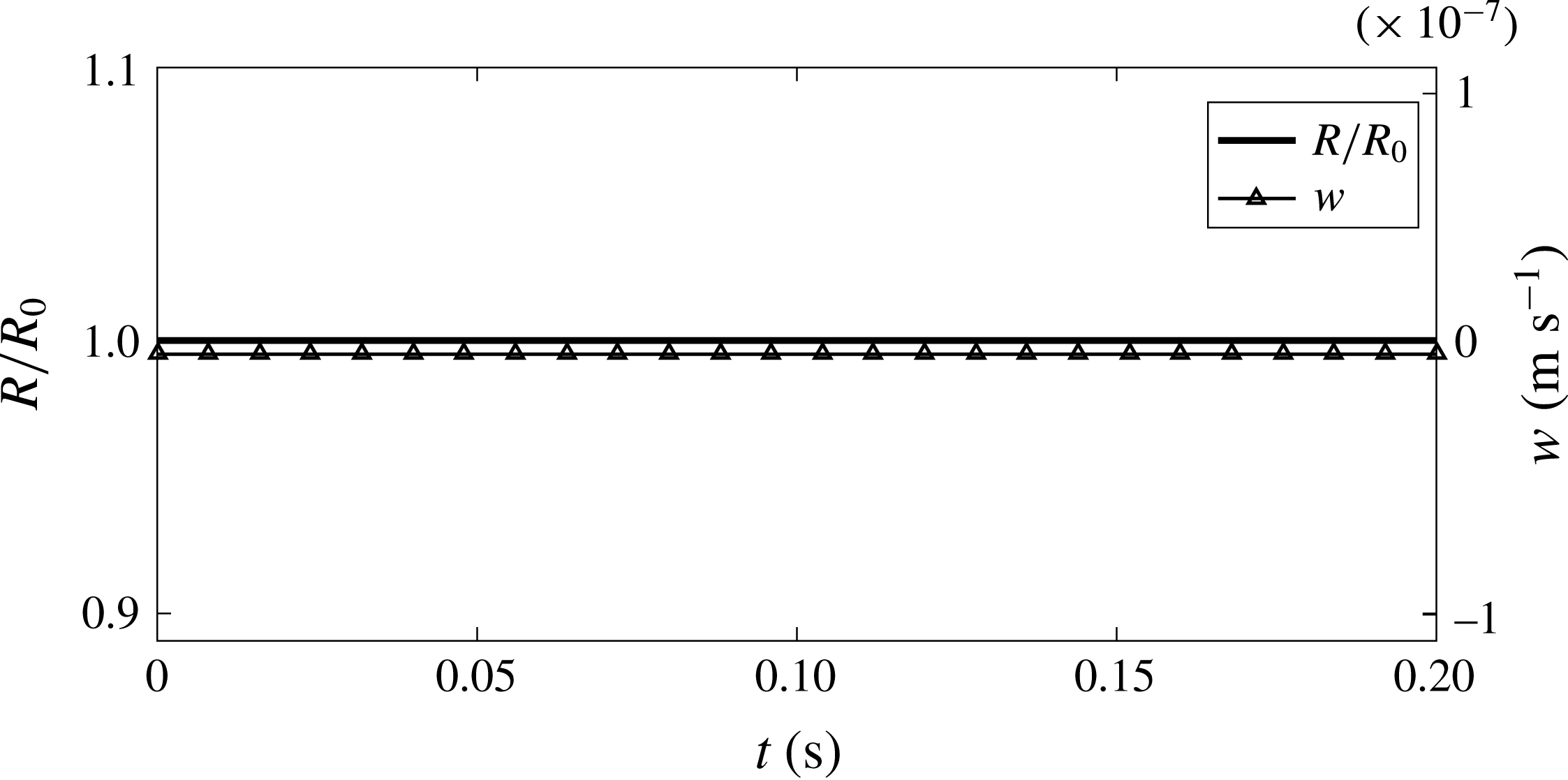
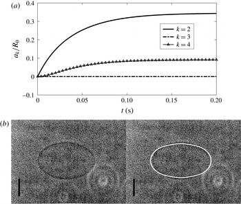
. As shown in figure 2, the radius of the bubble hardly changes, so that the compressibility of gas does not play a role and the membrane stress dominates the dynamics of the bubble. The applied electric field does not move the bubble, as shown in the time development of translational velocity in figure 2 and predicted in (2.58). The main effect of the applied electric field is to elongate the bubble. Figure 3(a) suggests the second- and fourth-order shape modes develop under the electric field and become stable to be a new shape within 0.2 s. This time scale is close to Kummrow & Helfrich’s result. Plotting the shape at the stable state based on the magnitudes of different shape modes and comparing with Kummrow & Helfrich’s observation, we find that the shapes agree well with each other (figure 3
b).
Time evolutions of radius (left
 $y$
-axis) and velocity (right
 $y$
-axis) of an encapsulated bubble with initial radius
 $R_{0}=23~\unicode[STIX]{x03BC}\text{m}$
and bending modulus
 $G_{b}=2.47\times 10^{-20}~\text{N}~\text{m}$
under a steady electric field with
 $E_{0}=10^{4}~\text{V}~\text{m}^{-1}$
.

(a) Time evolutions of shape modes for
 $k=2$
, 3 and 4 for an encapsulated bubble with initial radius
 $R_{0}=23~\unicode[STIX]{x03BC}\text{m}$
and bending modulus
 $G_{b}=2.47\times 10^{-20}~\text{N}~\text{m}$
under a steady electric field with
 $E_{0}=10^{4}~\text{V}~\text{m}^{-1}$
. (b) Comparison of the stable shape under
 $E_{0}=10^{4}~\text{V}~\text{m}^{-1}$
with the experimental observation by Kummrow & Helfrich (Reference Kummrow and Helfrich1991). The bar represents
 $20~\unicode[STIX]{x03BC}\text{m}$
.

The dynamic equations for the shape modes (2.59) and (2.60) are linear oscillation equations in which the coefficient before
 $a_{k}$
is related to the natural frequencies. Therefore, substituting (3.3) into (2.59) or (2.60) and neglecting the time variation of
 $R$
and viscous effects, we obtain the natural frequencies of the shape modes associated with the bending modulus
 $$\begin{eqnarray}f_{k}^{bend}=\frac{1}{2\unicode[STIX]{x03C0}}\sqrt{k(k-1)(k+1)^{2}(k+2)\frac{G_{b}}{\unicode[STIX]{x1D70C}R_{0}^{5}}}.\end{eqnarray}$$
Notice that the electric stress includes the terms with
 $a_{k}$
, implying the applied electric field will change the natural frequency of the shape mode. Here we take the second-order shape mode as an example and derive its natural frequency, including the effect of electric field, as
 $$\begin{eqnarray}\displaystyle f_{2}^{ele} & = & \displaystyle \frac{1}{2\unicode[STIX]{x03C0}}\left[k(k-1)(k+1)^{2}(k+2)\frac{G_{b}}{\unicode[STIX]{x1D70C}R_{0}^{5}}\right.\nonumber\\ \displaystyle & & \displaystyle +\,\frac{6E_{0}^{2}}{35\unicode[STIX]{x1D70C}R_{0}}\frac{\unicode[STIX]{x1D700}_{0}\unicode[STIX]{x1D700}_{ex}(\unicode[STIX]{x1D700}_{ex}-\unicode[STIX]{x1D700}_{in})(52\unicode[STIX]{x1D700}_{ex}^{2}-109\unicode[STIX]{x1D700}_{ex}\unicode[STIX]{x1D700}_{in}+27\unicode[STIX]{x1D700}_{in}^{2})}{(2\unicode[STIX]{x1D700}_{ex}+\unicode[STIX]{x1D700}_{in})^{3}}\nonumber\\ \displaystyle & & \displaystyle +\,\frac{2q_{1}E_{0}}{35\unicode[STIX]{x1D70C}R_{0}}\frac{\unicode[STIX]{x1D700}_{ex}(44\unicode[STIX]{x1D700}_{ex}^{2}+506\unicode[STIX]{x1D700}_{ex}\unicode[STIX]{x1D700}_{in}-325\unicode[STIX]{x1D700}_{in}^{2})}{(2\unicode[STIX]{x1D700}_{ex}+\unicode[STIX]{x1D700}_{in})^{3}}\nonumber\\ \displaystyle & & \displaystyle -\left.\frac{2q_{1}^{2}}{35\unicode[STIX]{x1D70C}R_{0}}\frac{128\unicode[STIX]{x1D700}_{ex}^{3}+772\unicode[STIX]{x1D700}_{ex}^{2}\unicode[STIX]{x1D700}_{in}+417\unicode[STIX]{x1D700}_{ex}\unicode[STIX]{x1D700}_{in}^{2}-62\unicode[STIX]{x1D700}_{in}^{3}}{(2\unicode[STIX]{x1D700}_{ex}+\unicode[STIX]{x1D700}_{in})^{3}(4\unicode[STIX]{x1D700}_{ex}+3\unicode[STIX]{x1D700}_{in})}\right]^{1/2},\end{eqnarray}$$
where
 $k=2$
. With the parameters adopted in the present work, the modification to the natural frequency due to the electric field is less than 1 %. Hence we can calculate the natural frequency of the shape mode simply by (3.5) to be
 $f_{2}^{bend}=2.6~\text{Hz}$
. Nevertheless, (3.6) indicates that the effect of an electric field on the natural frequency will enhance as its magnitude
 $E_{0}$
increases. In (3.6), the third and fourth terms in square brackets, which are related to
 $q_{1}$
, are calculated to be much smaller than the second term, related to
 $E_{0}^{2}$
, according to the results below (see figure 4). The sign of the second term is determined by the sign of
 $(\unicode[STIX]{x1D700}_{ex}-\unicode[STIX]{x1D700}_{in})$
if
 $\unicode[STIX]{x1D700}_{ex}$
and
 $\unicode[STIX]{x1D700}_{in}$
are significantly different, as in the case of a bubble or a drop. Therefore, the natural frequency increases with increasing electric field for a bubble with
 $\unicode[STIX]{x1D700}_{ex}>\unicode[STIX]{x1D700}_{in}$
, and this trend is opposite for a drop with
 $\unicode[STIX]{x1D700}_{ex}<\unicode[STIX]{x1D700}_{in}$
. These characteristics have been demonstrated by Lee & Kang (Reference Lee and Kang1999).
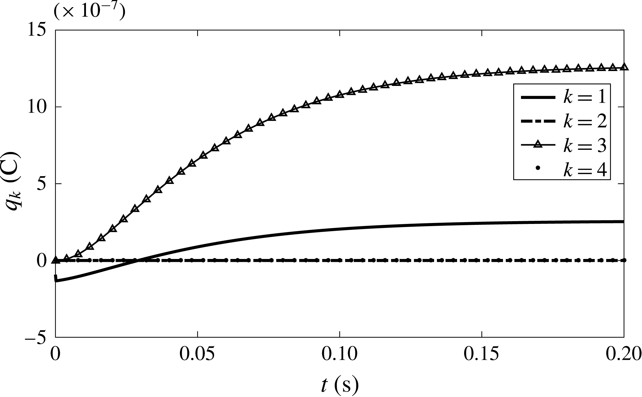
Distribution of free charge at the interface versus time for an encapsulated bubble with initial radius
 $R_{0}=23~\unicode[STIX]{x03BC}\text{m}$
and bending modulus
 $G_{b}=2.47\times 10^{-20}~\text{N}~\text{m}$
under a steady electric field with
 $E_{0}=10^{4}~\text{V}~\text{m}^{-1}$
.

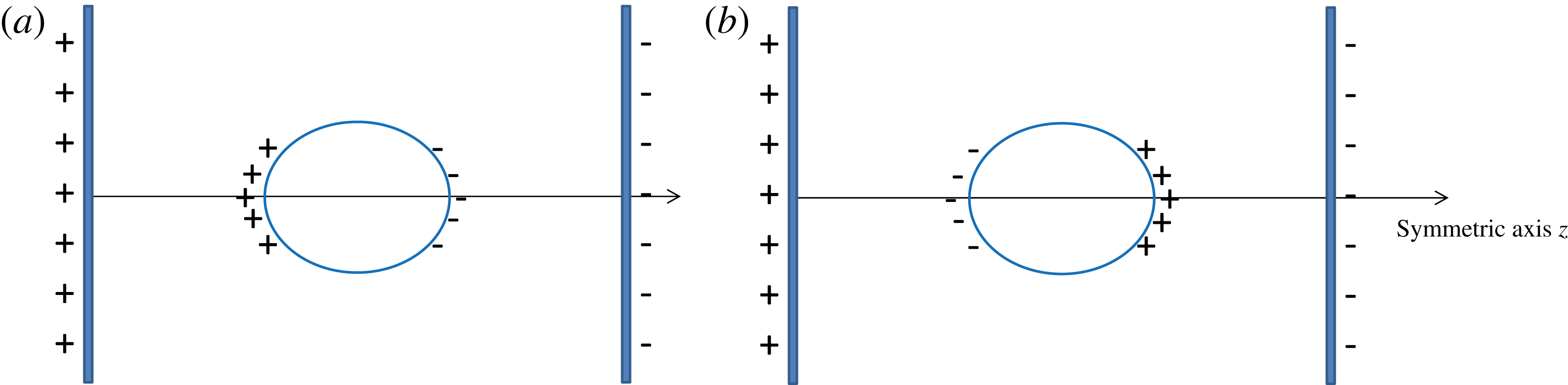
Sketch of charge distribution for both (a) negative
 $q_{1}$
and (b) positive
 $q_{1}$
.

The time evolutions of charge distributions are shown in figure 4. At the beginning,
 $q_{1}$
is negative, which corresponds to the distribution as figure 5(a), i.e. the negative charge accumulates at the pole closer to the negative plate electrode while the positive charge is closer to the positive plate electrode. The sign of
 $q_{1}$
transits to be positive as time goes. The transition of the sign can be explained by investigating (2.73). Since the radius does not change (figure 2) and
 $q_{2}$
remains zero (figure 4), the terms including
 ${\dot{R}}$
and
 $q_{2}$
are eliminated here. Substituting
 $A_{1}$
(2.13) and
 $B_{1}$
(2.14), (2.73) becomes
 $$\begin{eqnarray}\displaystyle \dot{q}_{1}+\frac{6{\dot{a}}_{2}}{5R}q_{1} & = & \displaystyle \frac{3E_{0}(\unicode[STIX]{x1D700}_{ex}\unicode[STIX]{x1D705}_{in}-\unicode[STIX]{x1D700}_{in}\unicode[STIX]{x1D705}_{ex})-(2\unicode[STIX]{x1D705}_{ex}+\unicode[STIX]{x1D705}_{in})\unicode[STIX]{x1D700}_{0}q_{1}}{2\unicode[STIX]{x1D700}_{ex}+\unicode[STIX]{x1D700}_{in}}\nonumber\\ \displaystyle & & \displaystyle +\,\frac{6a_{2}}{5R}\frac{E_{0}(\unicode[STIX]{x1D700}_{ex}\unicode[STIX]{x1D705}_{ex}+2\unicode[STIX]{x1D700}_{in}\unicode[STIX]{x1D705}_{ex}-3\unicode[STIX]{x1D700}_{ex}\unicode[STIX]{x1D705}_{in})+q_{1}\unicode[STIX]{x1D700}_{0}(\unicode[STIX]{x1D705}_{ex}+\unicode[STIX]{x1D705}_{in})}{2\unicode[STIX]{x1D700}_{ex}+\unicode[STIX]{x1D700}_{in}}.\end{eqnarray}$$
At the initial time when the charge has not moved and the deformation is not obvious (
 $a_{2}$
is small), the sign of
 $q_{1}$
is determined by the sign of
 $\unicode[STIX]{x1D700}_{ex}\unicode[STIX]{x1D705}_{in}-\unicode[STIX]{x1D700}_{in}\unicode[STIX]{x1D705}_{ex}$
. For the present case with gas inside and water outside,
 $\unicode[STIX]{x1D700}_{ex}\unicode[STIX]{x1D705}_{in}-\unicode[STIX]{x1D700}_{in}\unicode[STIX]{x1D705}_{ex}<0$
, so that
 $q_{1}<0$
. As
 $a_{2}$
increases, the bubble becomes prolate and the second term on the right-hand side of (3.7) dominates the first term, and
 $q_{1}$
becomes positive. Referred to figure 3(a), the criterion of
 $a_{2}/R_{0}$
for the sign transition is approximately 0.19. The value of
 $q_{3}$
is zero at the beginning and develops to be positive with larger magnitude than
 $q_{1}$
, since
 $q_{3}$
is induced by
 $a_{2}$
and
 $a_{4}$
according to (2.75), which becomes appreciable as time goes (figure 3
a). The even order of
 $q_{k}$
, such as
 $k=2$
and 4, remains zero, as they are induced by the odd order of shape mode, such as
 $a_{3}$
, which does not appear in the present case.
3.2 Membrane with hyperelasticity and bending rigidity
For a general membrane with hyperelasticity and bending rigidity, we add the hyperelastic stress to the bubble in § 3.1 by setting
 $G_{s}=0.15~\text{N}~\text{m}^{-1}$
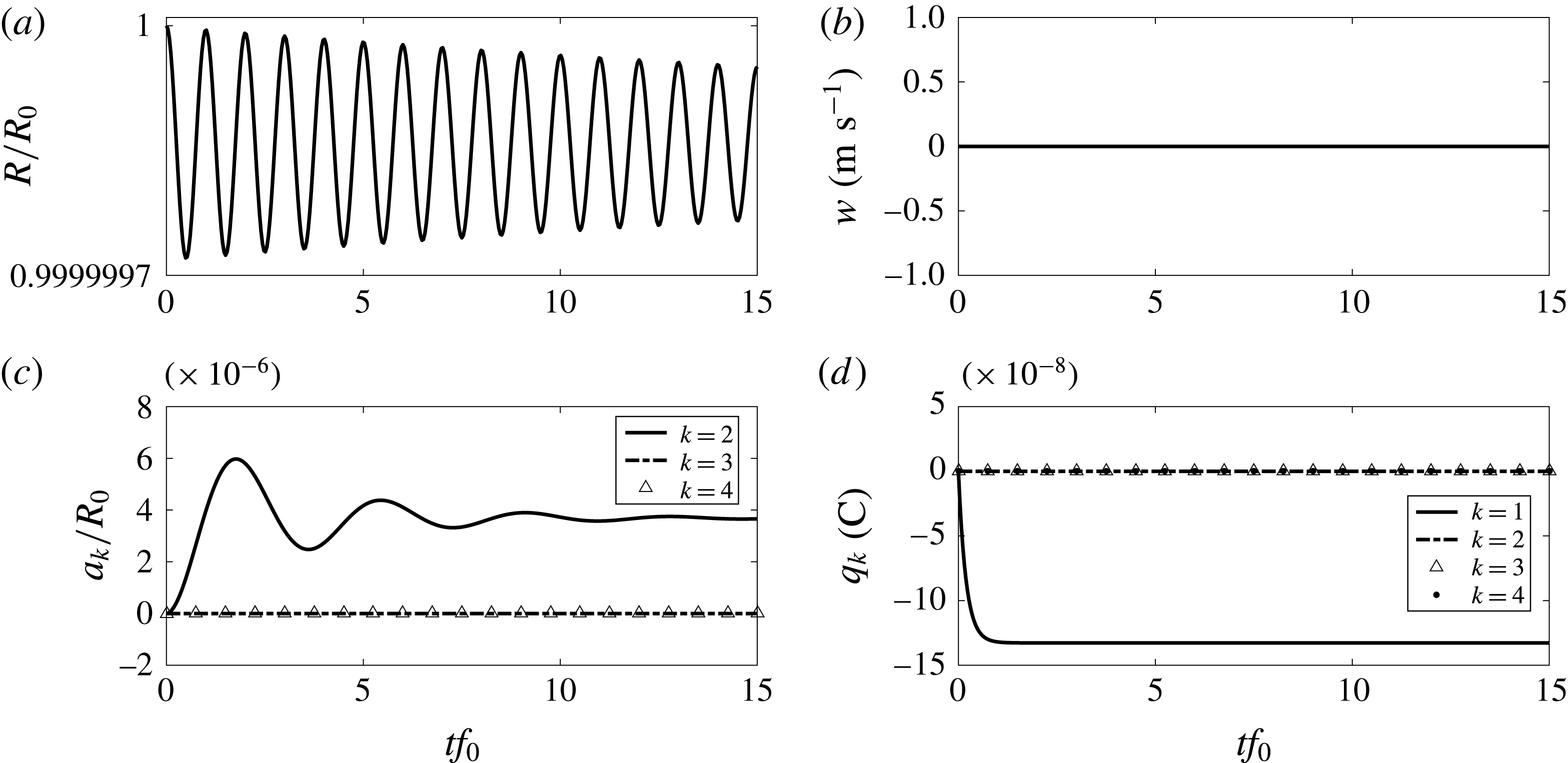
, which is a moderate elastic modulus for an encapsulated bubble in medical applications (Unnikrishnan & Klibanov Reference Unnikrishnan and Klibanov2012), and keeping other parameters unchanged. The time developments of radius, translational velocity, shape modes and charge distributions are shown in figure 6. The time is scaled by the zeroth-order natural frequency calculated by Liu et al. (Reference Liu, Sugiyama, Takagi and Matsumoto2012) as
 $$\begin{eqnarray}f_{0}=\frac{1}{2\unicode[STIX]{x03C0}}\sqrt{\frac{3\unicode[STIX]{x1D6E4}p_{\infty }}{\unicode[STIX]{x1D70C}R_{0}^{2}}+\frac{12G_{s}}{\unicode[STIX]{x1D70C}R_{0}^{3}}}.\end{eqnarray}$$
Under the resistance from elastic stress, the radius oscillation is at an infinitesimal amplitude and damping due to the liquid viscosity. The translational velocity remains zero. Especially, the deformation of the bubble is much smaller than that of a bubble coated with a bending-resistant membrane. Owing to the small magnitude of shape modes,
 $q_{1}$
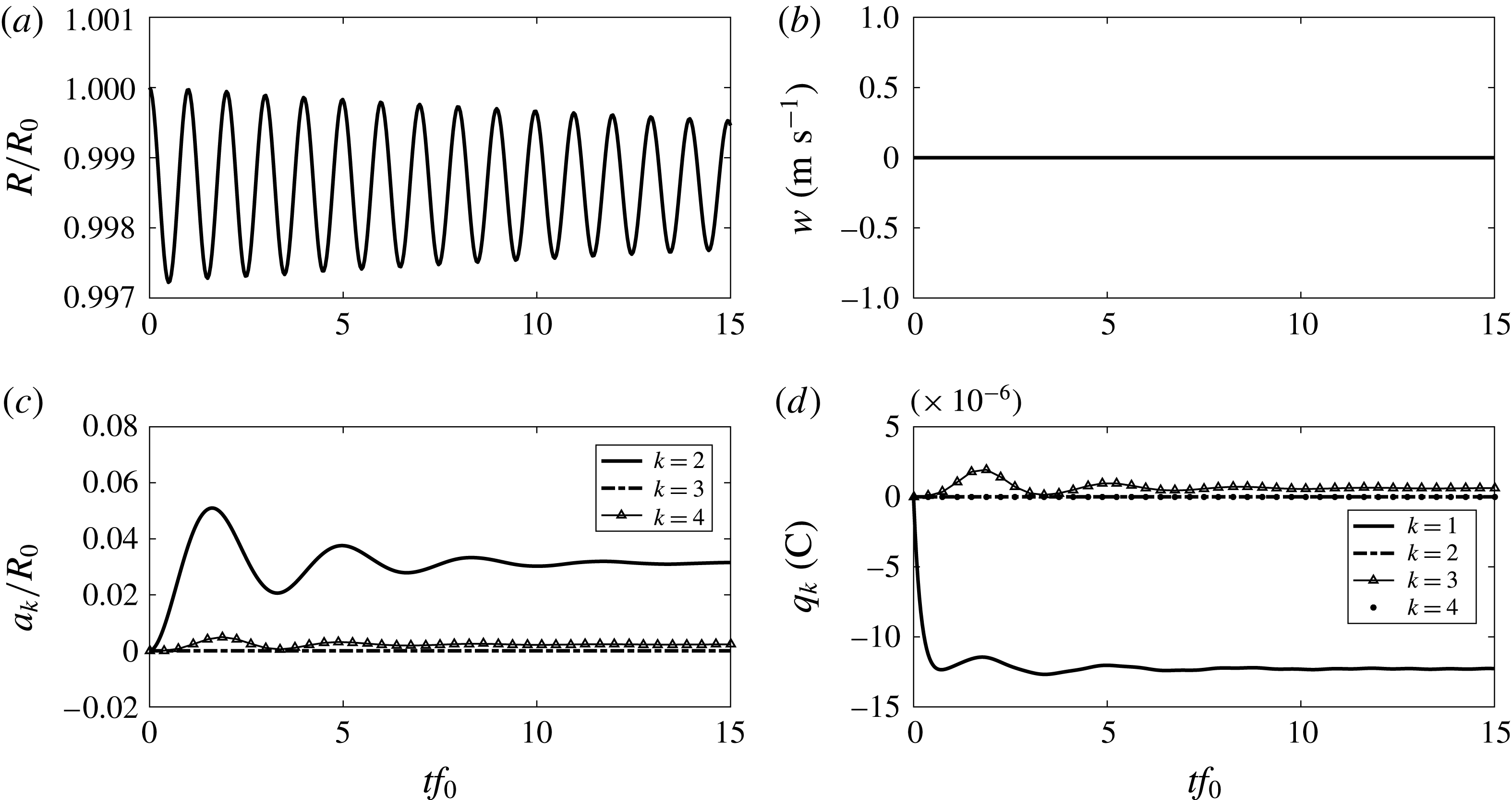
becomes stable to a negative value and other mode distribution is not triggered. For a bubble encapsulated by a hyperelastic membrane, a steady electric field has a small effect on its dynamics. As a result, it is not easy to obtain the characteristic parameters such as elastic modulus, natural frequency, etc. using a steady electric field. Even if we increase the electric field, e.g. by applying
 $E_{0}=10^{6}~\text{V}~\text{m}^{-1}$
, as shown in figure 7, the deformation at the stable state is an order of magnitude smaller than that of the bubble with bending rigidity only (see figure 3
a).
Time evolutions of (a) radius, (b) translational velocity, (c) shape modes and (d) charge distribution for an encapsulated bubble, with initial radius
 $R_{0}=23~\unicode[STIX]{x03BC}\text{m}$
, elastic modulus
 $G_{s}=0.15~\text{N}~\text{m}^{-1}$
and bending modulus
 $G_{b}=2.47\times 10^{-20}~\text{N}~\text{m}$
under a steady electric field with
 $E_{0}=10^{4}~\text{V}~\text{m}^{-1}$
.

Time evolutions of (a) radius, (b) translational velocity, (c) shape modes and (d) charge distribution for an encapsulated bubble, with initial radius
 $R_{0}=23~\unicode[STIX]{x03BC}\text{m}$
, elastic modulus
 $G_{s}=0.15~\text{N}~\text{m}^{-1}$
and bending modulus
 $G_{b}=2.47\times 10^{-20}~\text{N}~\text{m}$
under a steady electric field with
 $E_{0}=10^{6}~\text{V}~\text{m}^{-1}$
.

The results above suggest that the effect of a steady electric field on encapsulated bubble dynamics is small. To explore the effect of a temporally oscillatory electric field, we apply
 $$\begin{eqnarray}E_{0}=E_{a}\sin (2\unicode[STIX]{x03C0}f_{e}t),\end{eqnarray}$$
where
 $E_{a}$
is the amplitude of the oscillatory electric field and
 $f_{e}$
is the oscillatory frequency. This electric field is spatially uniform. Similar to the radial mode, the second-order shape mode has a quadratic relation with the electric field
 $E_{0}$
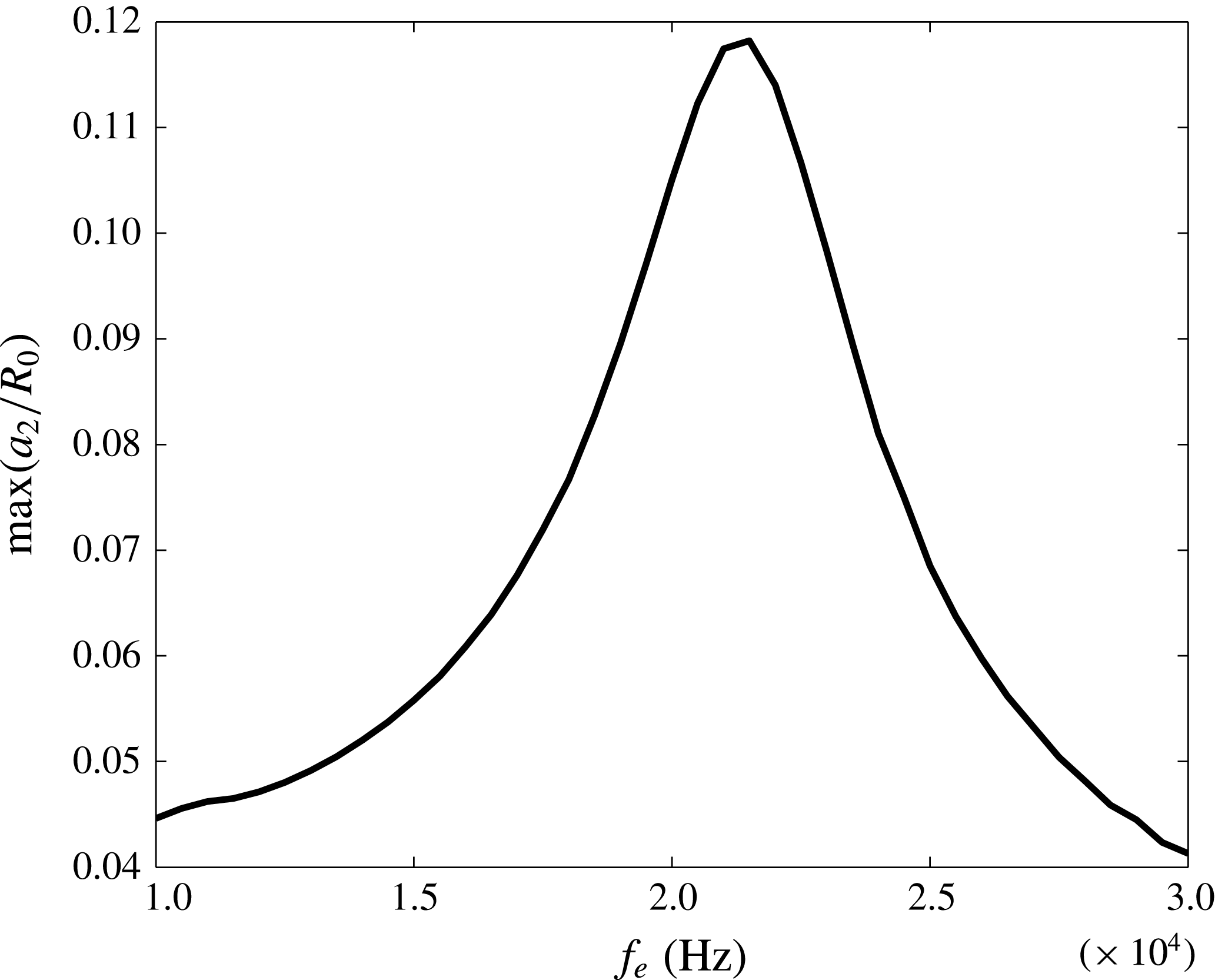
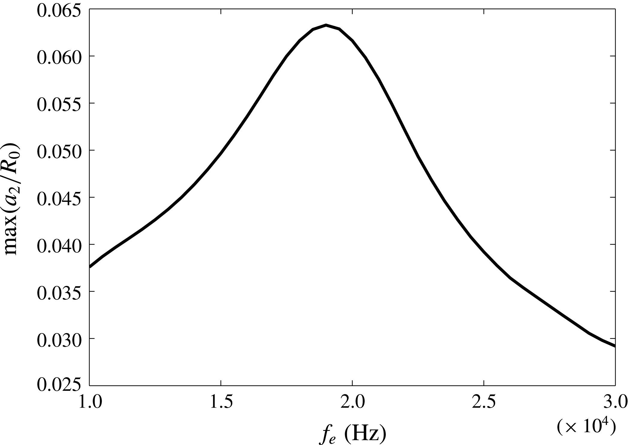
in the dynamic equation (2.59). If we set the electric frequency equal to half of the natural frequency, the shape oscillation is resonant and thus the amplitude of the shape mode is enlarged. The natural frequency of shape modes for the encapsulated bubble is calculated by Liu et al. (Reference Liu, Sugiyama, Takagi and Matsumoto2012) as
 $$\begin{eqnarray}f_{k}^{hp}=\frac{1}{2\unicode[STIX]{x03C0}}\sqrt{2(k-1)(k+1)(k+2)\frac{G_{s}}{\unicode[STIX]{x1D70C}R_{0}^{3}}\frac{(2k^{2}+2k-3)(k^{2}+k-1+\unicode[STIX]{x1D710})G_{b}+6G_{s}R_{0}^{2}}{(k^{2}+k-1+\unicode[STIX]{x1D710})G_{b}+2(2k^{2}+2k-1)G_{s}R_{0}^{2}}},\end{eqnarray}$$
which is
 $f_{2}=45.2~\text{kHz}$
for the present bubble. Accordingly, we set
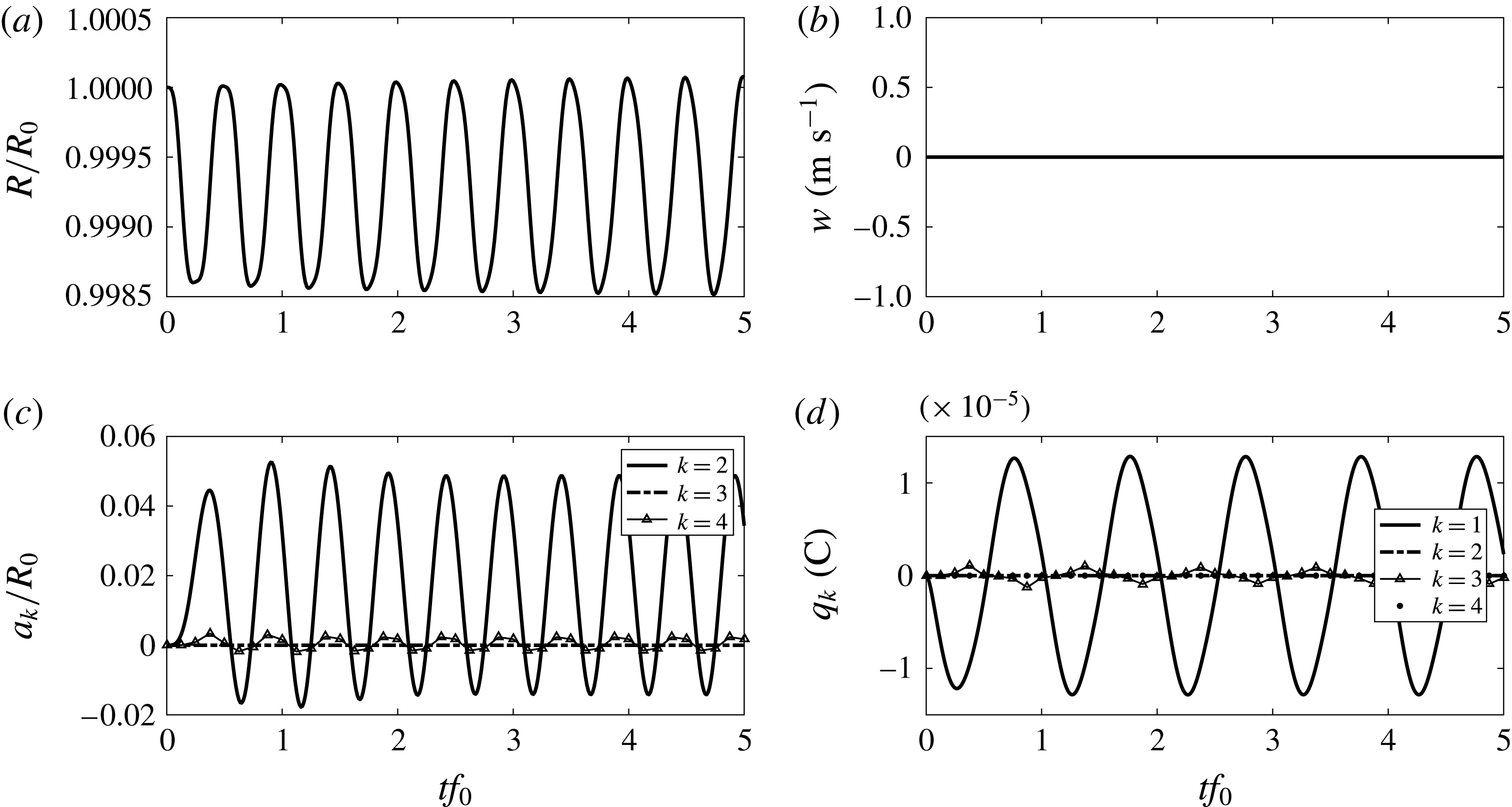
 $f_{e}=22.6~\text{kHz}$
and find in figure 8 that, although the radius still oscillates at a small amplitude, the second-order shape mode oscillates continuously with an amplitude twofold larger than the stable magnitude under a steady electric field (figure 7
c). The oscillation of the second-order shape mode reveals the prolate–oblate transition denoted by
 $a_{2}>0$
and
 $a_{2}<0$
, respectively. The underlying mechanism is the resonance between the electric frequency and the natural frequency of the shape mode, different from that for a vesicle discussed in Yamamoto et al. (Reference Yamamoto, Aranda-Espinoza, Dimova and Lipowsky2010), for which the prolate–oblate transition is attributed to displacement currents, which redirect the electric fields normal towards the membrane. The displacement currents dominate the conduction currents when the inverse Maxwell–Wagner time
 $\unicode[STIX]{x1D714}_{MW}=(\unicode[STIX]{x1D705}_{ex}+\unicode[STIX]{x1D705}_{in})/[\unicode[STIX]{x1D700}_{0}(\unicode[STIX]{x1D700}_{ex}+\unicode[STIX]{x1D700}_{in})]$
is lower than the electric frequency. In the present case,
 $\unicode[STIX]{x1D714}_{MW}$
is calculated to be
 $7\times 10^{5}$
Hz, higher than the electric frequency we choose, of the order of
 $O(10^{4})$
being the natural frequency of the bubble. This is the reason that we do not include displacement currents in our model.
Time evolutions of (a) radius, (b) translational velocity, (c) shape modes and (d) charge distribution for an encapsulated bubble, with initial radius
 $R_{0}=23~\unicode[STIX]{x03BC}\text{m}$
, elastic modulus
 $G_{s}=0.15~\text{N}~\text{m}^{-1}$
and bending modulus
 $G_{b}=2.47\times 10^{-20}~\text{N}~\text{m}$
under an oscillatory electric field with
 $E_{0}=10^{6}\sin (2\unicode[STIX]{x03C0}f_{e}t)~\text{V}~\text{m}^{-1}$
, where
 $f_{e}=22.6~\text{kHz}$
.

To obtain the natural frequency of the shape mode for an encapsulated bubble, we can modulate the electric frequency to induce resonance. As an example, we take a gas bubble whose natural frequency of the shape mode has been widely used (Lamb Reference Lamb1932):
 $$\begin{eqnarray}f_{k}^{gas}=\frac{1}{2\unicode[STIX]{x03C0}}\sqrt{(k-1)(k+1)(k+2)\frac{\unicode[STIX]{x1D6FE}}{\unicode[STIX]{x1D70C}R_{0}^{3}}},\end{eqnarray}$$
where
 $\unicode[STIX]{x1D6FE}$
is the coefficient of surface tension, set as
 $0.0729~\text{N}~\text{m}^{-1}$
for the gas–water interface. The model in § 2 is applicable by assigning
 $F_{n}$
as the surface tension:
 $$\begin{eqnarray}F_{n}=\unicode[STIX]{x1D6FE}\unicode[STIX]{x1D735}\boldsymbol{\cdot }\boldsymbol{n}=\frac{2\unicode[STIX]{x1D6FE}}{R}+\unicode[STIX]{x1D6FE}\mathop{\sum }_{k=2}^{\infty }(k+2)(k-1)\frac{a_{k}}{R^{2}}P_{k}(\cos \unicode[STIX]{x1D703}).\end{eqnarray}$$
The interface of a gas bubble is free slip, so that the shear stress
 $F_{t}=0$
.
We investigate a gas bubble with the same size as above,
 $R_{0}=23~\unicode[STIX]{x03BC}\text{m}$
, for which the natural frequency of the second-order shape mode is
 $f_{2}^{gas}=42.7~\text{kHz}$
calculated by (3.11). Sweeping the electric frequency and recording the maximal amplitude of the second-order shape mode after the transient state, we find that the maximum of amplitude appears at around 21 kHz (figure 9), which is half of its natural frequency. In the same way, we find that the maximum for the encapsulated bubble with
 $R_{0}=23~\unicode[STIX]{x03BC}\text{m}$
,
 $G_{s}=0.15~\text{N}~\text{m}^{-1}$
and
 $G_{b}=2.47\times 10^{-20}~\text{N}~\text{m}$
is at approximately 20 kHz (figure 10), slightly less than half of the natural frequency we calculated above (
 $f_{2}^{hp}/2=22.6~\text{kHz}$
by (3.10)). The smaller value is attributed to the significant effect of viscosity for an encapsulated bubble, which makes the resonant frequency smaller than the natural frequency without considering the effect of viscosity. Nevertheless, frequency modulation of an oscillatory electric field is a feasible way to estimate the natural frequencies of shape modes. In addition, the maximum
 $a_{2}$
at resonance is more than twice the stable
 $a_{2}$
under a steady electric field, making it easier to detect bubble deformation.
The maximal amplitude of the second-order shape mode under various electric field frequencies for a gas bubble with
 $R_{0}=23~\unicode[STIX]{x03BC}\text{m}$
.

The maximal amplitude of the second-order shape mode under various electric field frequencies for an encapsulated bubble with
 $R_{0}=23~\unicode[STIX]{x03BC}\text{m}$
,
 $G_{s}=0.15~\text{N}~\text{m}^{-1}$
and
 $G_{b}=2.47\times 10^{-20}~\text{N}~\text{m}$
.

4 Conclusion
In this paper, we have proposed a leaky dielectric model for investigating the dynamics of an encapsulated bubble in an electric field. The applied electric field is spatially uniform and temporally constant or oscillatory. Outside the bubble, we solve a potential flow field with a viscous pressure correction. The electric field and flow field are coupled through force balance on the bubble surface, including electric, hydrodynamic traction and membrane stresses. The system of equations and interface conditions, including the charge transport equation on the bubble surface, are approximated using Legendre polynomials, representing radial, translational and shape oscillations.
Our results for a bubble coated with a bending-resistant membrane show that it undergoes elongated deformation subject to a steady electric field, whose shape agrees well with the observation by Kummrow & Helfrich (Reference Kummrow and Helfrich1991) with the same parameters. The distribution of charge on the bubble surface is determined by the magnitude of shape modes and the sign of
 $\unicode[STIX]{x1D700}_{ex}\unicode[STIX]{x1D705}_{in}-\unicode[STIX]{x1D700}_{in}\unicode[STIX]{x1D705}_{ex}$
. The effect of electric field on the natural frequency is well predicted by our model.
For a hyperelastic membrane with bending rigidity, our results show that the deformation and radial oscillation of an encapsulated bubble are not as visible under a steady applied electric field. By modulating the frequency of an oscillatory electric field, on the other hand, we can induce shape mode resonance. Since the deformation is more significant, natural frequencies of the shape model can be estimated directly with less error.
Acknowledgements
This work was supported by the National Natural Science Foundation of China (11772196, 11372191, 11302128, 11402174), the Natural Science and Engineering Research Council (NSERC) and the Fields Institute of Canada, and the president’s fund – research start-up fund from the Chinese University of Hong Kong, Shenzhen.
Appendix A. Relations of the Legendre polynomials
The orthogonal relations of the Legendre polynomials are used throughout this paper. The Legendre polynomials
 $P_{k}(\cos \unicode[STIX]{x1D703})$
and
 $P_{k}^{1}(\cos \unicode[STIX]{x1D703})$
are simply written as
 $P_{k}$
and
 $P_{k}^{1}$
in this appendix. We have
 $$\begin{eqnarray}\displaystyle & \displaystyle \int _{-1}^{1}P_{k}P_{l}\,\text{d}(\cos \unicode[STIX]{x1D703})=0,\quad \text{when }k\not =l, & \displaystyle\end{eqnarray}$$
 $$\begin{eqnarray}\displaystyle & \displaystyle (P_{1})^{2}={\textstyle \frac{1}{3}}(P_{0}+2P_{2}), & \displaystyle\end{eqnarray}$$
 $$\begin{eqnarray}\displaystyle & \displaystyle (P_{1}^{1})^{2}={\textstyle \frac{2}{3}}(P_{0}-P_{2}), & \displaystyle\end{eqnarray}$$
 $$\begin{eqnarray}\displaystyle & \displaystyle \mathop{\sum }_{k=2}^{\infty }a_{k}P_{1}P_{k}=\mathop{\sum }_{k=1}^{\infty }\frac{k+1}{2k+3}a_{k+1}P_{k}+\mathop{\sum }_{k=3}^{\infty }\frac{k}{2k-1}a_{k-1}P_{k}, & \displaystyle\end{eqnarray}$$
 $$\begin{eqnarray}\displaystyle & \displaystyle \mathop{\sum }_{k=2}^{\infty }a_{k}P_{1}^{1}P_{k}^{1}=\mathop{\sum }_{k=1}^{\infty }\frac{(k+1)(k+2)}{2k+3}a_{k+1}P_{k}-\mathop{\sum }_{k=3}^{\infty }\frac{k(k-1)}{2k-1}a_{k-1}P_{k}, & \displaystyle\end{eqnarray}$$
 $$\begin{eqnarray}\displaystyle \mathop{\sum }_{k=2}^{\infty }a_{k}P_{1}P_{1}P_{k} & = & \displaystyle \mathop{\sum }_{k=0}^{\infty }\frac{(k+1)(k+2)}{(2k+3)(2k+5)}a_{k+2}P_{k}\nonumber\\ \displaystyle & & \displaystyle +\,\mathop{\sum }_{k=2}^{\infty }\frac{2k^{2}+2k-1}{(2k-1)(2k+3)}a_{k}P_{k}+\mathop{\sum }_{k=4}^{\infty }\frac{k(k-1)}{(2k-3)(2k-1)}a_{k-2}P_{k},\qquad\end{eqnarray}$$
 $$\begin{eqnarray}\displaystyle \mathop{\sum }_{k=2}^{\infty }a_{k}P_{1}P_{1}^{1}P_{k}^{1} & = & \displaystyle \mathop{\sum }_{k=0}^{\infty }\frac{(k+1)(k+2)(k+3)}{(2k+3)(2k+5)}a_{k+2}P_{k}\nonumber\\ \displaystyle & & \displaystyle +\,\mathop{\sum }_{k=2}^{\infty }\frac{k(k+1)}{(2k-1)(2k+3)}a_{k}P_{k}+\mathop{\sum }_{k=4}^{\infty }\frac{k(k-1)(k-2)}{(2k-3)(2k-1)}a_{k-2}P_{k}.\qquad\end{eqnarray}$$
Appendix B. The interfacial deflection in imposing the boundary condition of an electric field
Based on the axisymmetric coordinate we established, the gradient to the electric potential is written as
 $$\begin{eqnarray}\displaystyle \unicode[STIX]{x1D735}\unicode[STIX]{x1D713}=\boldsymbol{e}_{r}\frac{\unicode[STIX]{x2202}\unicode[STIX]{x1D713}}{\unicode[STIX]{x2202}r}+\boldsymbol{e}_{\unicode[STIX]{x1D703}}\frac{1}{r}\frac{\unicode[STIX]{x2202}\unicode[STIX]{x1D713}}{\unicode[STIX]{x2202}\unicode[STIX]{x1D703}}, & & \displaystyle\end{eqnarray}$$
where the subscripts ‘ex’ or ‘in’ are omitted temporarily for brevity. The projections of electric field to the normal and tangential directions are expressed as
 $$\begin{eqnarray}\displaystyle & \displaystyle \boldsymbol{n}\boldsymbol{\cdot }\unicode[STIX]{x1D735}\unicode[STIX]{x1D713}=\frac{\unicode[STIX]{x2202}\unicode[STIX]{x1D713}}{\unicode[STIX]{x2202}r}-\frac{1}{r^{2}}\frac{\unicode[STIX]{x2202}\unicode[STIX]{x1D713}}{\unicode[STIX]{x2202}\unicode[STIX]{x1D703}}\mathop{\sum }_{k=2}^{\infty }a_{k}P_{k}^{1}, & \displaystyle\end{eqnarray}$$
 $$\begin{eqnarray}\displaystyle & \displaystyle \boldsymbol{t}\boldsymbol{\cdot }\unicode[STIX]{x1D735}\unicode[STIX]{x1D713}=\frac{1}{r}\frac{\unicode[STIX]{x2202}\unicode[STIX]{x1D713}}{\unicode[STIX]{x2202}r}\mathop{\sum }_{k=2}^{\infty }a_{k}P_{k}^{1}+\frac{1}{r}\frac{\unicode[STIX]{x2202}\unicode[STIX]{x1D713}}{\unicode[STIX]{x2202}\unicode[STIX]{x1D703}}. & \displaystyle\end{eqnarray}$$
According to the forms of electric potential (2.11) and (2.12), the terms in (B 2) and (B 3) are expanded with respect to the interface deflection defined in (2.1) and (2.2) as follows:
 $$\begin{eqnarray}\displaystyle \frac{\unicode[STIX]{x2202}\unicode[STIX]{x1D713}_{ex}}{\unicode[STIX]{x2202}r} & = & \displaystyle -\left(E_{0}-\frac{2A_{1}R^{3}}{r^{3}}\right)P_{1}+\mathop{\sum }_{k=2}^{\infty }(k+1)\frac{A_{k}}{r^{k+2}}P_{k}\nonumber\\ \displaystyle & = & \displaystyle (-E_{0}+2A_{1})P_{1}-\frac{6A_{1}}{R}\mathop{\sum }_{k=2}^{\infty }a_{k}P_{1}P_{k}+\mathop{\sum }_{k=2}^{\infty }(k+1)\frac{A_{k}}{R^{k+2}}P_{k},\end{eqnarray}$$
 $$\begin{eqnarray}\displaystyle & \displaystyle \frac{1}{r}\frac{\unicode[STIX]{x2202}\unicode[STIX]{x1D713}_{ex}}{\unicode[STIX]{x2202}\unicode[STIX]{x1D703}}=-(E_{0}+A_{1})P_{1}^{1}-\mathop{\sum }_{k=2}^{\infty }\frac{A_{k}}{R^{k+2}}P_{k}^{1}, & \displaystyle\end{eqnarray}$$
 $$\begin{eqnarray}\displaystyle & \displaystyle \frac{\unicode[STIX]{x2202}\unicode[STIX]{x1D713}_{in}}{\unicode[STIX]{x2202}r}=-B_{1}P_{1}-\mathop{\sum }_{k=2}^{\infty }kB_{k}R^{k-1}P_{k}, & \displaystyle\end{eqnarray}$$
 $$\begin{eqnarray}\displaystyle & \displaystyle \frac{1}{r}\frac{\unicode[STIX]{x2202}\unicode[STIX]{x1D713}_{in}}{\unicode[STIX]{x2202}\unicode[STIX]{x1D703}}=-B_{1}P_{1}^{1}-\mathop{\sum }_{k=2}^{\infty }B_{k}R^{k-1}P_{k}^{1}. & \displaystyle\end{eqnarray}$$
Appendix C. Derivation of the right-hand side of (2.69)
We denote the right-hand side of (2.69) as
 $$\begin{eqnarray}D=\frac{\text{d}q}{\text{d}t}+q\unicode[STIX]{x1D735}_{s}\boldsymbol{\cdot }\bar{\boldsymbol{u}}\end{eqnarray}$$
and derive its detailed expression in this section.
First, write out the Lagrangian derivative as
 $$\begin{eqnarray}D=\frac{\unicode[STIX]{x2202}\widetilde{q}}{\unicode[STIX]{x2202}t}+(\bar{\boldsymbol{u}}\boldsymbol{\cdot }\unicode[STIX]{x1D735})\widetilde{q}+q\unicode[STIX]{x1D735}_{s}\boldsymbol{\cdot }\bar{\boldsymbol{u}},\end{eqnarray}$$
where
 $\widetilde{q}$
is the extension of
 $q$
to the neighbourhood of the interface, in order to calculate the time derivative and gradient. Decomposing
 $\bar{\boldsymbol{u}}$
into the tangential and normal components
 $\bar{\boldsymbol{u}}=\bar{\boldsymbol{u}}_{s}+\bar{\boldsymbol{u}}_{n}$
yields
 $$\begin{eqnarray}D=\frac{\unicode[STIX]{x2202}\widetilde{q}}{\unicode[STIX]{x2202}t}+(\bar{\boldsymbol{u}}_{n}\boldsymbol{\cdot }\unicode[STIX]{x1D735})\widetilde{q}+(\bar{\boldsymbol{u}}_{s}\boldsymbol{\cdot }\unicode[STIX]{x1D735})\widetilde{q}+q\unicode[STIX]{x1D735}_{s}\boldsymbol{\cdot }\bar{\boldsymbol{u}}.\end{eqnarray}$$
By using
 $\bar{\boldsymbol{u}}_{s}\boldsymbol{\cdot }\unicode[STIX]{x1D735}=\bar{\boldsymbol{u}}\boldsymbol{\cdot }\unicode[STIX]{x1D735}_{s}$
, the above final two terms can be combined and (C 3) is rewritten as
 $$\begin{eqnarray}D=\frac{\unicode[STIX]{x2202}\widetilde{q}}{\unicode[STIX]{x2202}t}+(\bar{\boldsymbol{u}}_{n}\boldsymbol{\cdot }\unicode[STIX]{x1D735})\widetilde{q}+\unicode[STIX]{x1D735}_{s}\boldsymbol{\cdot }(q\bar{\boldsymbol{u}}).\end{eqnarray}$$
Further decomposing
 $\bar{\boldsymbol{u}}$
into the tangential and normal components as
 $\bar{\boldsymbol{u}}=\bar{\boldsymbol{u}}_{s}+(\bar{\boldsymbol{u}}\boldsymbol{\cdot }\boldsymbol{n})\boldsymbol{n}$
,
 $$\begin{eqnarray}D=\frac{\unicode[STIX]{x2202}\widetilde{q}}{\unicode[STIX]{x2202}t}+(\bar{\boldsymbol{u}}_{n}\boldsymbol{\cdot }\unicode[STIX]{x1D735})\widetilde{q}+\unicode[STIX]{x1D735}_{s}\boldsymbol{\cdot }(q\bar{\boldsymbol{u}}_{s})+q(\unicode[STIX]{x1D735}_{s}\boldsymbol{\cdot }\boldsymbol{n})(\bar{\boldsymbol{u}}\boldsymbol{\cdot }\boldsymbol{n})+(\bar{\boldsymbol{u}}\boldsymbol{\cdot }\boldsymbol{n})\boldsymbol{n}\boldsymbol{\cdot }\unicode[STIX]{x1D735}_{s}q,\end{eqnarray}$$
the last term of which is zero due to orthogonality, so that
 $D$
becomes
 $$\begin{eqnarray}\displaystyle D=\frac{\unicode[STIX]{x2202}\widetilde{q}}{\unicode[STIX]{x2202}t}+(\bar{\boldsymbol{u}}_{n}\boldsymbol{\cdot }\unicode[STIX]{x1D735})\widetilde{q}+\unicode[STIX]{x1D735}_{s}\boldsymbol{\cdot }(q\bar{\boldsymbol{u}}_{s})+q(\unicode[STIX]{x1D735}_{s}\boldsymbol{\cdot }\boldsymbol{n})(\bar{\boldsymbol{u}}\boldsymbol{\cdot }\boldsymbol{n}). & & \displaystyle\end{eqnarray}$$
Referring to the method by Pereira et al. (Reference Pereira, Trevelyan, Thiele and Kalliadasis2007), who treated surfactant on a horizontal film, we extend their work to the charge on a spherical interface and rewrite (C 6) as
 $$\begin{eqnarray}\displaystyle D=\frac{\unicode[STIX]{x2202}q}{\unicode[STIX]{x2202}t}+\bar{\boldsymbol{u}}_{n}\boldsymbol{\cdot }\boldsymbol{e}_{\unicode[STIX]{x1D703}}\frac{1}{r}\frac{\unicode[STIX]{x2202}q}{\unicode[STIX]{x2202}\unicode[STIX]{x1D703}}+\unicode[STIX]{x1D735}_{s}\boldsymbol{\cdot }(q\bar{\boldsymbol{u}}_{s})+q(\unicode[STIX]{x1D735}_{s}\boldsymbol{\cdot }\boldsymbol{n})(\bar{\boldsymbol{u}}\boldsymbol{\cdot }\boldsymbol{n}), & & \displaystyle\end{eqnarray}$$
where the time derivative is regarded as at a fixed
 $\unicode[STIX]{x1D703}$
under the assumption that
 $\unicode[STIX]{x1D703}$
and the bubble interface (zero contour of
 $S$
) are a one-to-one map, which is true in the present case. The derivations to the terms in (C 7) are given below. Here we neglect the coupling effect of
 $a_{k}$
and
 $w$
on the charge transport, i.e. eliminate the terms with
 $a_{k}w$
. Thus we have
 $$\begin{eqnarray}\displaystyle \bar{\boldsymbol{u}}_{n}\boldsymbol{\cdot }\boldsymbol{e}_{\unicode[STIX]{x1D703}}\frac{1}{r}\frac{\unicode[STIX]{x2202}q}{\unicode[STIX]{x2202}\unicode[STIX]{x1D703}} & = & \displaystyle (\bar{\boldsymbol{u}}\boldsymbol{\cdot }\boldsymbol{n})\boldsymbol{n}\boldsymbol{\cdot }\boldsymbol{e}_{\unicode[STIX]{x1D703}}\frac{1}{r}\frac{\unicode[STIX]{x2202}q}{\unicode[STIX]{x2202}\unicode[STIX]{x1D703}}\nonumber\\ \displaystyle & = & \displaystyle -{\dot{R}}\mathop{\sum }_{k=2}^{\infty }\frac{a_{k}}{R}P_{k}^{1}\mathop{\sum }_{k=1}^{\infty }\frac{1}{R}q_{k}P_{k}^{1}\nonumber\\ \displaystyle & = & \displaystyle -\frac{{\dot{R}}q_{1}}{R^{2}}\mathop{\sum }_{k=2}^{\infty }a_{k}P_{1}^{1}P_{k}^{1}\nonumber\\ \displaystyle & = & \displaystyle -\frac{{\dot{R}}q_{1}}{R^{2}}\left[\mathop{\sum }_{k=1}^{\infty }\frac{(k+1)(k+2)}{2k+3}a_{k+1}P_{k}-\mathop{\sum }_{k=3}^{\infty }\frac{k(k-1)}{2k-1}a_{k-1}P_{k}\right]\nonumber\\ \displaystyle & = & \displaystyle P_{1}\left(-\frac{6}{5}q_{1}\frac{{\dot{R}}a_{2}}{R^{2}}\right)+P_{2}\left(-\frac{12}{7}q_{1}\frac{{\dot{R}}a_{3}}{R^{2}}\right)\nonumber\\ \displaystyle & & \displaystyle +\,\mathop{\sum }_{k=3}^{\infty }P_{k}\left[-\frac{{\dot{R}}q_{1}}{R^{2}}\left(\frac{(k+1)(k+2)}{2k+3}a_{k+1}-\frac{k(k-1)}{2k-1}a_{k-1}\right)\right]\,,\end{eqnarray}$$
 $$\begin{eqnarray}\displaystyle \unicode[STIX]{x1D735}_{s}\boldsymbol{\cdot }(q\bar{\boldsymbol{u}}_{s}) & = & \displaystyle P_{1}\left[\frac{2}{5}q_{1}\left(\frac{{\dot{a}}_{2}}{R}-\frac{{\dot{R}}a_{2}}{R^{2}}\right)+\frac{2}{5}q_{2}\left(-\frac{3w}{2R}+\frac{1}{R}\int _{R}^{\infty }s^{-1}T_{1}(s,t)\,\text{d}s\right)\right]\nonumber\\ \displaystyle & & \displaystyle +\,P_{2}\left[q_{1}\left(\frac{3w}{R}-\frac{2}{R}\int _{R}^{\infty }s^{-1}T_{1}(s,t)\,\text{d}s+\frac{6{\dot{a}}_{3}}{7R}-\frac{12}{7}\frac{{\dot{R}}a_{3}}{R^{2}}\right)\right.\nonumber\\ \displaystyle & & \displaystyle +\left.q_{3}\left(-\frac{9}{7}\frac{w}{R}+\frac{6}{7R}\int _{R}^{\infty }s^{-1}T_{1}(s,t)\,\text{d}s\right)\right]\nonumber\\ \displaystyle & & \displaystyle +\,\mathop{\sum }_{k=3}^{\infty }P_{k}\left\{q_{1}\left[\frac{k(k+1)}{2k+3}\left(\frac{{\dot{a}}_{k+1}}{R}-\frac{k{\dot{R}}a_{k+1}}{R^{2}}\right)\right.\right.\nonumber\\ \displaystyle & & \displaystyle +\left.\frac{(k-1)(k+1)}{2k-1}\left(\frac{{\dot{a}}_{k-1}}{R}-(k-2)\frac{{\dot{R}}a_{k-1}}{R^{2}}\right)\right]\nonumber\\ \displaystyle & & \displaystyle +\left.\left(q_{k+1}\frac{k(k+1)}{2k+3}-q_{k-1}\frac{k(k+1)}{2k-1}\right)\left(-\frac{3w}{2R}+\frac{1}{R}\int _{R}^{\infty }s^{-1}T_{1}(s,t)\,\text{d}s\right)\right\}\,,\nonumber\\ \displaystyle & & \displaystyle\end{eqnarray}$$
 $$\begin{eqnarray}\displaystyle q(\unicode[STIX]{x1D735}_{s}\boldsymbol{\cdot }\boldsymbol{n})(\bar{\boldsymbol{u}}\boldsymbol{\cdot }\boldsymbol{n}) & = & \displaystyle P_{1}\left[q_{1}\left(\frac{2{\dot{R}}}{R}+\frac{8}{5}\frac{a_{2}{\dot{R}}}{R^{2}}+\frac{4}{5}\frac{{\dot{a}}_{2}}{R}\right)\right]\nonumber\\ \displaystyle & & \displaystyle +\,P_{2}\left[q_{1}\left(\frac{30}{7}\frac{a_{3}{\dot{R}}}{R^{2}}+\frac{6{\dot{a}}_{3}}{7R}-\frac{4a_{2}}{7R^{2}}\int _{R}^{\infty }s^{-1}T_{1}(s,t)\,\text{d}s\right)+q_{2}\frac{2{\dot{R}}}{R}\right]\nonumber\\ \displaystyle & & \displaystyle +\,\mathop{\sum }_{k=3}^{\infty }P_{k}\left\{q_{1}\left[\frac{k+1}{2k+3}\left(k(k+3)\frac{a_{k+1}{\dot{R}}}{R^{2}}+\frac{2{\dot{a}}_{k+1}}{R}\right)\right.\right.\nonumber\\ \displaystyle & & \displaystyle +\,\frac{k}{2k-1}\left((k+1)(k-2)\frac{a_{k-1}{\dot{R}}}{R^{2}}+\frac{2{\dot{a}}_{k-1}}{R}\right)\nonumber\\ \displaystyle & & \displaystyle -\left.\left.\frac{2k(k+1)}{(2k-1)(2k+3)}\frac{a_{k}}{R^{2}}\int _{R}^{\infty }s^{-1}T_{1}(s,t)\,\text{d}s\right]+q_{k}\frac{2{\dot{R}}}{R}\right\}\!.\end{eqnarray}$$