Poverty as a multi-dimensional concept

Poverty is a complex and multi-dimensional phenomenon that, in Europe at least, is normally defined relative to the living standards of the society in which it is found. Following Henry Mayhew (Reference Mayhew1851) and Charles Booth (Reference Booth1892), Seebohm Rowntree (Reference Rowntree1901) grappled with the complexity, distinguishing between different categories of poverty and noting the need to take account of social conditions, diet and health as well as income in assessing living standards. Much later, Peter Townsend (Reference Townsend1979) argued that poverty was not the lack of income necessary to purchase a basket of goods but rather the lack of resources to participate fully in society that resulted, through a process he termed ‘structuration’, from a variety of resource allocation systems operating in society. The measures created by Townsend have since been critically assessed, developed and refined by scholars such as Piachaud (Reference Piachaud1981), Mack and Lansley (Reference Mack and Lansley1985) and Gordon et al. (Reference Gordon, Levitas, Pantazis, Patsios, Payne, Townsend, Adelman, Ashworth, Middleton, Bradshaw and Williams2000). Increasingly priority is being given to material deprivation and to environmental aspects of people's lives over shortfalls in income (Callan et al., Reference Callan, Nolan and Whelan1993; Nolan and Whelan, Reference Nolan and Whelan1996; Layte et al., Reference Layte, Nolan and Whelan2001). For Ringen (Reference Ringen1988), income is merely an indirect measure of poverty that is truly experienced as the unavoidable low consumption that denies people access to a normal way of life.

Townsend's conception of poverty was inherently relative in that participation refers to engagement in ‘the activities, customs and diets commonly approved by society’ (Reference Townsend1979: 88). While Townsend (with Brian Abel-Smith, Reference Townsend and Abel-Smith1965) had earlier popularised the notion of relative, as opposed to absolute, poverty, he was not the first to make this distinction. Adam Smith noted, for example, that:

It is also apparent, from this quotation, that Smith saw shame and stigma as being inherent components of poverty, aspects that still loom large in the experience of poor people in Britain today (Lister, Reference Lister2004; Women's Budget Group, 2005). Indeed, Sen (Reference Sen1999) argues that the shame that results from poor people being unable to realise basic capabilities consistent with the society in which they live is universal and absolute, manifest in all societies irrespective of the level of economic development.

The increasing availability of data, and most notably the creation of extensive longitudinal datasets, has focused attention on poverty dynamics and the analysis of the length and frequency of spells, and added to an understanding of the complexity of the phenomenon (Walker with Ashworth, Reference Walker and Ashworth1994; Jenkins and Rigg, Reference Jenkins and Rigg2001; Rigg and Sefton, Reference Rigg and Sefton2006; Maggio, Reference Maggio2004; Fouarge and Layte, Reference Fouarge and Layte2005; Layte and Whelan, Reference Layte and Whelan2003; Whelan et al., Reference Whelan, Layte and Maitre2002). Dynamic analyses have demonstrated that poverty is much more widespread than indicated by cross-sectional statistics; that transient, recurrent and permanent poverty may differ in kind and in their effects; and that the risk events associated with poverty are more prevalent than spells of actual poverty. This suggests that social structures and individual agency may protect some people against the onset of poverty. Hobfoll (Reference Hobfoll1998) has argued, drawing on the Conservation of Resources (COR) theory of psycho-social stress, that people with greater resources (defined in terms of social support, financial means, material goods, psychological resilience) will be less vulnerable when such resources are threatened or lost while, conversely, others with few resources may get caught in cumulative spirals of resource loss, a phenomenon already documented in qualitative research (Walker and Collins, Reference Walker, Collins, Scott, Treas and Richards2003; Kempson, Reference Kempson1996).

Certain social and psychological supports that protect people against poverty can be eroded should poverty occur, adding further momentum to downward spirals of insecurity. Good physical and mental health, social capital and competence and civic engagement are all casualties of poverty and may, in certain circumstances, be compounded when mediated by the negative characteristics of poor places such as dilapidated infrastructure, isolation, crime and red-lining.

Poverty, of course, has a political dimension. Indeed, Piachaud (Reference Piachaud1987) among others argues that poverty is inherently political since it carries the imperative to respond to eradicate it. After a long period of neglect in Britain, poverty has moved to the political centre-stage since New Labour took office in 1997. Most notable was the 1999 commitment to eradicate child poverty (Blair, Reference Blair and Walker1999): a political objective that has now been accepted by the Conservative opposition (Callan et al., Reference Callan, Benson, Coward, Davis, Gill, Grant, Percival, Rowthorn, Rowley and Anderson2006). Political definitions of poverty, while influenced by academic research, are also affected by practical expediency. Forty-one indicators of poverty and social exclusion are currently used by the UK Department for Work and Pensions separately to measure changes in poverty (DWP, 2006a). In so doing, government implicitly accepts the multi-dimensional nature of poverty, but has lacked a means of simultaneously measuring and aggregating these measures to produce a stable composite measure. Moreover, it plans to prioritise three measures of poverty: a relative measure, a quasi-absolute measure based on freezing a relative measure in terms of real purchasing power, and a measure of material deprivation to capture different aspects of poverty. The three measures together also serve to direct attention from unpalatable features of a relative income measure, namely that it provides an upwardly moving target in situations of overall economic growth: one that is given further momentum in situations where growth is accompanied by growing inequality.

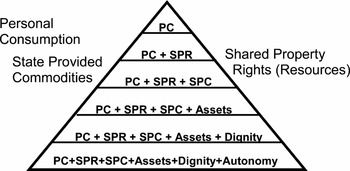
Ringen (Reference Ringen1988) draws attention to the measurement assumption and the income assumption in poverty research. The former refers to the belief that poverty exists and as such can be measured. The latter presumes that poverty can be measured in terms of a deficit in income in relation to needs, an assumption that becomes increasingly untenable if poverty is defined as the complex multi-dimensional phenomenon described above. Baulch (Reference Baulch1996) has illustrated the problem with reference to a pyramid of concepts (Figure 1). Moving down the pyramid takes increasing account of aspects of poverty that define it as a meaningful social phenomenon. In terms of measurement, the most frequently used measures lie at the top of the pyramid since they are more straightforward to operationalise.

Figure 1.

Baulch's Pyramid Source: Baulch (Reference Baulch1996).

Personal consumption is placed at the top of the pyramid, although this is typically measured with reference to personal or, more usually, household income since this is more easily measured.Footnote ¹ The concept of poverty gradually increases in scope to include shared property rights, state-provided commodities, assets, dignity and autonomy at the bottom of the pyramid. The implication of the diagram is that the various dimensions are strictly additive, although empirically this is unlikely ever to be the case. Indeed, a major challenge of the current research is to formulate the nature of the relationship between these various dimensions. Moreover, it is probable that the dimensions lie in a causative sequence which will require specification.

In summary, while it is widely appreciated that poverty is an inherently multi-dimensional concept, this multi-dimensionality has been lost, weakened or distorted when poverty is measured. This has not just been the result of political expediency but the absence of any method by which the holistic nature of poverty can be captured in a way that facilitates measurement over time. The partial measures used to date necessarily fail adequately to do justice to the experience of poor people and, to the extent that they distort through omission, may result in implementation of inappropriate policies.

What is required is the use of statistical techniques that represent the dimensionality of the concept in a stable fashion, an approach that will ultimately require access to comprehensive datasets with reliable measures. Below we outline an initial attempt to create a comprehensive poverty index for Great Britain using a novel statistical technique that has rarely been used in poverty studies. Some exceptions that we know of are Layte et al. (Reference Layte, Nolan and Whelan2000), Kuklys (Reference Kuklys2004), Haase and Pratschke (Reference Haase and Pratschke2005) and Ministry of Social Development (2002).Footnote ²

Furthermore, we are not in the present study engaged in causal analysis. The recognition that poverty (or any other social phenomenon) is multi-dimensional is to accept that the experience/phenomenon at any point in time is simultaneously shaped by a person's position or score on each of the constituent dimensions. It is possible, indeed probable, that all the dimensions of poverty are causally related and we are currently investigating this with a full structural equation model. However, because causality involves temporal ordering, this means that a person's score in time t ₀ on one dimension will affect/cause their score on another dimension only in time t ₁, t ₂ and so on. Thus causality is irrelevant to measuring a person's score on multiple dimensions at a given point in time and hence, in this article, we employ a purely measurement model rather than a causal structural model.

A new approach to measurement

In much previous quantitative research on poverty the data reduction technique of factor analysis has been used (see, for example, Calandrino, Reference Calandrino2003, and the review by Haase and Pratschke, Reference Haase and Pratschke2005). Simply put, this technique usually takes as input a large number of indicator variables and creates a smaller number of dimensions or ‘factors’ by examining the correlations between variables. These factors represent a simpler description of the data and usually can be readily interpreted by observing which variables cluster together to form the dimensions. So, for example, in poverty research material deprivation scales have been created by using factor analysis on sets of items that households possess and indices developed by examining which types of item cluster together on which particular factors (for example, Calandrino, Reference Calandrino2003). These dimensions are usually forced to be orthogonal (independent), although this does not have to be the case.

There are some problems with this methodology. We deal with three here. First, composite indicators created using factor analysis – which are essentially weighted summations of individual variables – are sensitive to errors in measurement of the original variables. This gets amplified when the original variables are used to create the factor scores and is further compounded when the factor solutions are used across several years (see Loehlin, Reference Loehlin1992). Such measures cannot be meaningfully compared over time, with the result that trends in the various dimensions of poverty cannot be securely established.

Secondly, the factors often have to be rotated to allow a useful interpretation. That is, the original solution has to be operated on in such a way as to ease elucidation of the results or to fit with some theoretical framework. As a result of these rotations, factors are not necessarily comparable over time or space (Haase and Pratschke, Reference Haase and Pratschke2005).

Thirdly, factor analysis is essentially an exploratory technique. No strong theoretical justification is required in deciding which variables to include or exclude from the analysis, and the researcher has little control over how the variables form the resulting factors. Thus, factor analysis can be useful in other contexts where an exploratory approach is required.

A structural equation model (SEM) has the potential to overcome some of these problems. Like factor analysis, a SEM reduces a large number of variables to a smaller number of factors. However, the variables are conceptualised as observed manifestations of underlying or latent concepts. Each observed variable in a SEM also has an error term associated with it, allowing measurement error to be isolated and controlled for in a way that is impossible with factor analysis. But, most importantly, a SEM requires a strong theoretical justification before the model is specified. Thus the researcher decides which observed variables are to be associated with which latent unobserved factors in advance. This avoids the problems of instability and rotated solutions prevalent in factor analysis.

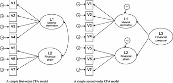
There are two fundamental types of SEM used to measure or test the validity of latent concepts: first- and second-order confirmatory factor analysis models (CFAs).Footnote ³ A first-order CFA simply attempts to measure underlying latent concepts. The left side of Figure 2 shows a simple CFA, which has two latent unobserved variables: L1, material deprivation; and L2, financial strain. L1 is measured by the observed variables V1 to V4, and L2 is measured by variables V5 to V7. The single-headed arrows represent coefficients or loadings in the model and are usually shown in standardised form much like beta coefficients in regression analysis.Footnote ⁴ The covariance between material deprivation (L1) and financial strain (L2) is represented by the double-headed arrow. The associated error terms are shown as the circles labelled e1 to e7. Using statistical techniques such as maximum likelihood and making assumptions about the distributions of the variables and error terms in the model, the coefficients and covariances can be estimated. In all SEMs a variety of fit statistics is available to assess the validity of the models constructed (see Klein, Reference Klein2005; Byrne, Reference Byrne2001). Usually it is assumed that the observed variables in the model are continuous and that the distribution of the variables is multi-variate normal. However, many studies treat categorical variables as continuous in SEM analyses (see Byrne, Reference Byrne2001: 70–72, for a discussion of these issues). More recently, available software is beginning to allow the explicit modelling of categorical, binary and censored variables (such as MPlus).

Figure 2.

A simple first-order CFA model A simple second-order CFA model

This basic model can be taken a stage further: a second-order CFA, as shown on the right of Figure 2 where another latent variable L3 is used to capture a latent concept, financial pressure, theorised to relate simultaneously to both L1 and L2. It will be noted that L1 and L2 now have residuals associated with them (res1 and res2). Models of this kind can be made as complex as necessary to describe real-world situations and employ many latent variables and various interactions between them. Furthermore, in both types of model, scores can be generated for the unobserved latent variables. These scores are analogous to the factor scores obtained using factor analysis, but without the limitations previously discussed. It is this higher-order CFA approach that we attempt below.Footnote ⁵

To summarise the advantages of this approach:

1. • Unlike standard factor analysis the researcher determines the underlying factors or latent constructs and their observed manifestations

2. • It allows modelling along strong theoretically based lines

3. • Complex relationships can be specified between these theoretical constructs

4. • It allows estimates of the unobserved variables to be calculated

5. • Error terms can be correlated or uncorrelated allowing greater flexibility

Defining the measurement models

The analysis utilises data from the British Household Panel Study (BHPS). The BHPS commenced in 1991 with an initial sample of around 10,000 individuals resident in some 5,000 households. These individuals have subsequently been re-interviewed each year and the sample has also been extended to include more households from Scotland and Wales and to embrace Northern Ireland. While the data can be weighted to provide an accurate picture of life in Great Britain or the United Kingdom at different points in time, this analysis is restricted to Great Britain (England, Scotland and Wales) to facilitate measurement of trends. The analysis covers the period 1991−2003 (that is, BHPS waves 1 to 13) and draws on information concerning the following topics: income, finances and benefits; stress; material deprivation; general housing and neighbourhood characteristics; and social exclusion and civic participation. Individuals under 18 years of age are excluded from the sample analysed (although the relationship between adult and child poverty is explored in Tomlinson et al., Reference Tomlinson, Walker and Williams2007).

While the BHPS is widely used in poverty research (for example, Jenkins and Rigg, Reference Jenkins and Rigg2001; Ermisch et al., Reference Ermisch, Francesconi and Pevalin2001; Jenkins and Cappallari, Reference Jenkins, Cappellari, Jenkins and Micklewright2007), there are a number of shortcomings the most important of which is that the data are not always consistent or collected for all waves. For example, the civic participation and social isolation variables are only available for alternate waves, while the housing and neighbourhood variables used are only included from wave 6 onwards. Similarly, the material deprivation variables, which were limited at the beginning of the survey, were significantly augmented from wave 6. Thus we are forced to limit our analysis to odd years 1991, 1993, 1995 and so on, and to divide our analysis into two parts. The first employs a relatively simple model to exploit data for the full period 1991 to 2003, while the second uses a more comprehensive model that takes advantage of the better data available from wave 6 onwards. The latter model conveniently coincides with the first eight years of the Blair government (1997, 1999, 2001 and 2003).

Finally, as with any secondary analysis, the analyst is constrained by the variables included in the dataset. Almost inevitably, key variables are omitted while the variables available constitute only imprecise indices of the concepts of interest.

Model 1 covering the period 1991 to 2003

As noted above, the creation of a structural equation model usually relies on some strong theoretical orientation that is specified in advance. Unlike factor analysis, we cannot just enter all the variables and see what will happen. We have to decide in advance on the latent concepts (factors) that characterise poverty, and specify which of the variables we observe are associated with which factors. In our case, rather than a strong theory, we have a pyramid-like framework of concepts (Figure 1) that the literature suggests may be manifestations or inherent outcomes of the experience of being in poverty. The objective in handling the large range of possible permutations of concepts is to arrive at a balanced model: that is, one in which more weight is given to items at the top of the pyramid (like income, material and financial variables) than to those at the bottom (social exclusion, civic participation, psychological wellbeing and the environment), while ensuring that the latter still have a significant impact on the index.

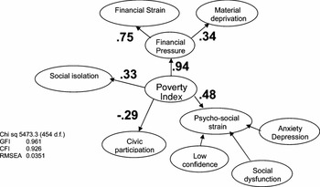
Figure 3 presents a second-order CFA model fitted to the BHPS data consistently available for alternate years from 1991 to 2003. It comprises several sets of indicators related to several latent concepts or dimensions that constitute the multi-dimensional poverty indicator (referred to from now on as the Poverty Index or PI). For simplicity's sake, only selected standardised coefficients between the major latent concepts and the overall index are shown.Footnote ⁶ Each major dimension is now described in turn.

Figure 3.

CFA model 1, waves 1–13, standardised coefficients shown

Financial strain (FINSTRAIN)

Several articles referred to in the introduction stress the importance of income-based measures of poverty, augmented here by indicators of the perceived financial situation of the household, the sense of being in financial hardship. Financial strain, the first dimension, is an almost self-evident manifestation of poverty, certainly one that is widely documented, that comes at the top of the poverty pyramid along with income as a primary indicator of privation. The variables used to capture this concept include whether a housing payment had been missed in the last 12 months (binary), whether respondents considered their financial status to be good/bad (using a five-point scale) and whether it had been getting better/worse over the last year (a three-point scale). The intention was that these variables should capture both long-term and the more immediate difficulties of budgeting, and the variables were all recoded so that a high value relates to a financially worse scenario. Income is also included on this latent variable (recoded as logarithm of equivalised household incomeFootnote ⁷).

Material deprivation (MATDEP)

There is a large body of work on the importance of including material deprivation in any measure of poverty (see Jenkins and Cappallari, Reference Jenkins, Cappellari, Jenkins and Micklewright2007; Whelan and Maitre, Reference Whelan and Maitre2005; Willetts, Reference Willetts2006, for example). The measures available in the BHPS are generally limited to the ownership of certain possessions with no reference made to whether respondents attribute lack of ownership to personal preference or inadequate resources. The raft of such indicators of material wellbeing include several binary variables each set to 1 if the household where the respondent lives does not possess a: CD player, VCR, washing machine, tumble dryer, microwave oven, dishwasher, personal computer, central heating or have use of a car (or to 0 if the items are available). Income is also included on this latent variable in the same format as for financial strain.Footnote ⁸

We have kept material deprivation conceptually distinct from financial strain as it represents the real effects of long-term financial hardship on the household rather than the personal financial strain itself. In other words, it captures the essence of not being able to afford things or being able to replace worn-out items such as electronic goods or kitchen appliances. Financial strain reflects monetary strain, which may be somewhat different and apply in different circumstances. For example, a household may be under financial strain because of high mortgage payments, but may have a well-equipped house.Footnote ⁹ Material and financial deprivation were also linked to the PI by another latent variable representing overall financial and material deprivation.Footnote ¹⁰ This represents the combined effects of long-term and short-term ‘financial pressure’.

Social isolation (SOCISOL)

The third dimension is that of social isolation, a trait seen both as a manifestation or consequence of poverty and as a risk factor linked with downward spirals into poverty and marginalisation (for example, Gallie et al., Reference Gallie, Paugam and Jacobs2003). Once a person is marginalised, the effect becomes self-reinforcing and it is difficult to escape either in terms of labour market security or poverty. Cattell (Reference Cattell2001) also investigates the linkages between social networks, poverty and health and has found complex relationships between the three. The BHPS includes variables indicating whether the respondent has someone who will listen to them, help them in a crisis, relax with, who appreciates them and who comforts them. In this analysis these variables were coded so that the most isolated score the highest (1 indicates they have no-one, 0 otherwise).

Civic participation (CIVIC)

Related to social isolation, we also include the converse concept of civic participation since the literature suggests that people in poverty will be excluded from civic participation and have weak social networks and social capital (Cattell, Reference Cattell2001; Gordon et al., Reference Gordon, Levitas, Pantazis, Patsios, Payne, Townsend, Adelman, Ashworth, Middleton, Bradshaw and Williams2000; Pantazis et al., Reference Pantazis, Gordon and Levitas2006). Civic participation is captured in the BHPS by two variables that count the number of organisations from a given list of which the respondent is a member and in which he or she is active. The list of 13 organisations is as follows: political party, trade union, environmental group, parents association, tenants or residents group, religious group, voluntary service, community group, social group, sports club, women's institute, women's group, other organisation. High scores indicate higher civic participation.

Psychological strain (PSYSTRAIN)

Psychological wellbeing could be seen as a cause or a consequence of poverty (Payne, Reference Payne, Pantazis, Gordon and Levitas2006). There have been a number of studies that have found an association between mental ill-health and poverty (for instance, Weich and Lewis, Reference Weich and Lewis1998; Whitley et al., Reference Whitley, Gunnell, Dorling and Smith1999). Many of the medical and psychological studies treat mental ill-health as the dependent variable, including several that explore the effects of poverty on children's psychological health (see, for example, Aber et al., Reference Aber, Bennett, Conley and Li1997; Evans, Reference Evans2004), while much social policy research focuses on the negative effects of mental illness on incomes. We assume here that psychological strain is a component towards the bottom of our pyramid of concepts and that it can be entered into a comprehensive poverty index.

Psychological strain is measured using the General Health Questionnaire set of 12 items (GHQ12) with the four-point scales being recoded to a binary with 1 suggesting ill-health and 0 otherwise.Footnote ¹¹ Following Shevlin and Adamson (Reference Shevlin and Adamson2005), we modelled psycho-social strain as a three-part model combining anxiety/depression (items 2, 5, 6, 9), social dysfunction (1, 3, 4, 7, 8) and loss of confidence (10 and 11). This produces a much better fit than using all 12 items loading on just one latent variable.

As indicated by the relative size of the coefficients in the model (Figure 3), most weight in the PI is assigned to financial pressure, itself more closely allied to financial strain than to material deprivation. The coefficients themselves are determined through the modelling process that identifies the model that best fits the data. The PI more closely reflects the measures of psychological strain than it does social isolation, while civic participation is similar in importance to social isolation, but, as anticipated, has the reverse effect on the PI (with high values lowering the PI score).

Model 2 covering the period 1997 to 2003

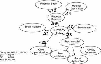
The more detailed data available in wave 6 onwards allow us to add another dimension, ‘environment’ (ENVIRON): a place-based aspect of poverty that captures housing and neighbourhood conditions, and to refine certain of the other dimensions (Figure 4). The binary housing variables included in the environment dimension are: whether the house in which a respondent resided suffered from bad light, bad heating, leaks, rotting wood, and/or damp. Neighbourhood variables included more objective measures appertaining to noise from neighbours, noise from the street, crime levels and lack of space, and more subjective ones recording whether the respondent liked the area or not and whether they would like to move away. Both sets of measures are coded to 1 for the most negative option and 0 otherwise to construct the environment dimension which supplants psychological strain as the second most important component in the PI index.

Figure 4.

CFA model 2, waves 7–13, standardised coefficients shown

The new material deprivation component additionally includes lack of access to cable/satellite TV, together with respondents’ assessment of whether their household could afford a holiday of one week once a year, to buy new clothes, to replace furniture or to feed visitors once a month, each coded as a binary variable (1 indicating lack of resources, 0 otherwise). Three binary variables are added to the social isolation dimension, with 1 indicating that the respondent could not go to someone outside the household to borrow money, find a job and to find help with depression. Financial strain, civic participation and psychological strain remain as in Model 1.

The models were run in AMOS 6.0 in conjunction with SPSS 14 on wave 1 of the BHPS for Model 1 and wave 7 for Model 2. Cross-sectional weighting was applied and listwise missing data deletion applied. Some correlations were allowed between error terms to improve fit in Model 2, although the coefficients do not change very much when this is done. The fit statistics are all quite respectable (GFI and CFI greater than 0.9 and RMSEA less than 0.05).

Scores for the PI were saved from both models and these form the basis of the analysis that follows. The procedure in AMOS 6.0 produces a set of linear equations that can be used to compute scores for all the latent concepts in the model, based on a weighted summation of the observed variables. The outcome is an equation the coefficients of which – termed ‘factor weights’ – were saved and used to compute scores for all successive waves.Footnote ¹² Therefore, factor weights from Model 1 in wave 1 were used to compute PI scores for all waves for the first set of analyses, while factor weights from Model 2 run in wave 7 were used for the second set.

Trends in multi-dimensional poverty

The twin methodological and substantive goals of the investigation require us first to consider the properties of the multi-dimensional measures. They are statistically sound, as already demonstrated by the test results, while their reliability should be ensured by holding the model structure constant over the period of the investigation, thereby avoiding the instability associated with factor analysis. In addition, a good indicator would be expected to be moderately stable over time (since it is unreasonable to expect poverty rates would vary wildly from year to year) and it should exhibit face validity in bearing some correlation with other accepted, if partial, indicators of poverty such as income.

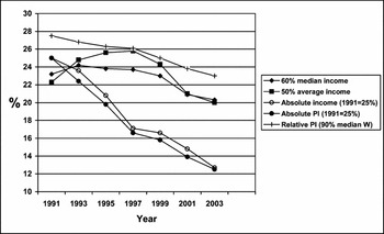
With the above considerations in mind, Figure 5 shows trends in conventional ‘relative’ and ‘absolute’ income poverty measures derived from the same BHPS data. The relative income measures show a pattern of stable or slightly increasing poverty during the John Major period 1992–97 and then a decline when New Labour took office from 1997 onwards while the absolute income measure, with the poverty threshold held constant in real terms, shows a continuous decline. The analogous PI-based measures, on the other hand, both show steady declines throughout the whole period, which is to be expected since a portion of the index is designed to capture aspects of poverty theorised to be more stable and less sensitive to short-term fluctuations in the national economic situation.

Figure 5.

Percentage poor by various measures, BHPS 1991–2003

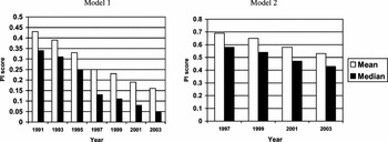
Figure 6 shows the mean and median PI score from Models 1 and 2 plotted across all odd year waves from wave 1 to 13. This is analogous to plotting the inverse of the trend in average equivalised household income used in traditional measures since, unlike income, the PI is a direct measure of poverty and high scores indicate extreme poverty. The mean score in Model 1 declines steadily throughout the period from around 0.43 to 0.16, consistent with the recorded fall in poverty rates and suggesting a general rise in social wellbeing, while the differences in the mean and median show that the distribution of the PI is slightly skewed, but less so than income alone. While it is clear that average PI fell significantly in absolute terms between 1991 and 2003 and that inequalities widened, perhaps especially during the last years of the Major government, it is not possible straightforwardly to assess the strength of this fall because the scores are not standardised in any way. Moreover, since a negative score is possible, meaning that a score of zero does not indicate an absence of poverty, it cannot be presumed that the average PI more than halved.

Figure 6.

Mean and median PI scores from the models

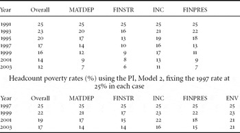
As with income-based measures, it is necessary to select a more or less arbitrary poverty threshold on the PI distribution to provide headcounts of poverty. Fixing the poverty rate at 25 per cent in 1991, in approximate accord with poverty rates according to traditional income based measures at the time, and using the associated PI score as a poverty threshold, the proportion of adults defined to be in poverty falls gradually over the whole period from the initial 25 per cent down to 12 per cent in 2003 (Table 1, column 1 and Figure 5). Moreover, it is possible to disaggregate the contribution made to this trend by the individual components. The subsets of the coefficients used to calculate the overall score from the model were used to calculate scores for each component (Table 1 shows selected components). The material deprivation (MATDEP) and financial stain (FINSTR) components were calculated without income included (which was calculated as a separate effect, INC) while financial pressure (FINPRES) combined the coefficients for income, material deprivation and financial strain.

TABLE 1.

Headcount poverty rates (%) using the PI and selected components, Model 1, fixing the 1991 rate at 25% in each case

The results of this analysis reveal that poverty rates based on the financial strain and material deprivation components of the index both fell much faster than income, declining by three quarters as opposed to half from 25 per cent in 1991 to around 8 per cent in 2003. Poverty defined in terms of financial strain decreased more quickly in the early part of the period subsequently slowing as, to a less marked degree, did material deprivation, whereas the marked fall in poverty experienced as financial pressure – a product of the effects of income, financial strain and material deprivation – occurred slightly later during the last years of the Major era. The other components, psychological strain (PSYSTRAIN), civic participation (CIVIC) and social isolation (SOCISOL) all remained fairly constant throughout the period and were, additionally, less closely associated in the model with the composite poverty index. The major falls in the index were therefore largely due to improvements in people's material wellbeing and easing of financial strain.

The more comprehensive measure that it was possible to employ during the Blair era presents a subtly different picture (see Figure 6, right-hand side). Again, the mean PI score fell but with different scaling, from 0.69 in 1997 to around 0.53 in 2003, implying an overall improvement in wellbeing. This is reflected in the headcount poverty rate which (calculated in an analogous fashion to Model 1, Table 1) fell by almost a quarter. During this period, however, while material deprivation and poverty manifest as financial strain, both fell by 44 per cent and by more than other aspects of poverty; the decline in income poverty was of a similar order of magnitude (36 per cent), presumably reflecting the significant policy shift to targeting poverty through increases in benefits and tax credits (see Table 1). Psychological strain, civic participation and social isolation again remained stable, but a decline in environmental or place-based poverty was evident, falling by about a sixth from 25 to 21 per cent.

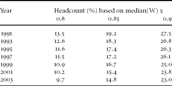
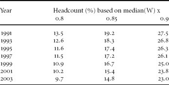
Reflecting Sen's analysis of capabilities and shame, the PI used in the foregoing analysis reflects both absolute and relative conceptualisations of poverty. The income measure is deflated, which removes the tendency with the absolute measures for people to be floated out of poverty simply as a result of economic growth. The measures of material deprivation are socially salient but are not weighted to take account of market penetration, while indices of strain are measured in absolute terms. It is possible to assess poverty rates relative to the entire distribution of PI scores in which case the PI would best be interpreted as a measure of wellbeing. To achieve this requires a slightly modified approach since it is necessary to normalise the PI before determining the poverty threshold values (see Appendix). Given that the PI has been shown to fall over the entire study period and its inverse – wellbeing – to rise, it comes as no surprise that the fall in poverty rates when measured against median wellbeing is much reduced (Table 2): a fall of between a sixth or a third rather than a half. However, it is also apparent that the more severe the measure of poverty employed, the larger the proportionate fall in the headcount rate, suggesting that changes were progressive with the poorest of the poor gaining most.

TABLE 2.

Headcount poverty rates (%) using various relative indicators, Model 1

Briefly, to summarise: poverty, measured as a multi-dimensional concept, fell throughout the period in both absolute and relative terms driven by reductions in material deprivation and financial strain rather than by increases in income per se.

The distribution of poverty

Having established trends in multi-dimensional poverty, it is appropriate for both substantive and methodological reasons to consider its distribution and correlates. Suffice, here, to focus on the association with income and its distribution by demographic group.

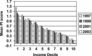
It will already be apparent from the structure of the measurement models and the fact that income poverty fell less markedly than other kinds of poverty that the PI is only moderately associated with income. Typically, in any one year, the correlation between the PI and the logarithm of household equivalised income is about 0.46, with income explaining no more than around 23 per cent of the variance of the PI. This is, of course, consistent with Ringen's (Reference Ringen1988) assertion above that income is an indirect and imperfect measure of poverty. Nevertheless, as anticipated, when the BHPS sample is divided into deciles according to equivalised household income, the average PI score falls consistently with increasing income decile (Figure 7).

Figure 7.

Mean PI from Model 2 by income deciles, 1997–2003

Figure 7 also reveals that the average PI score declined across the income distribution between 1997 and 2003. The biggest absolute falls were observed among the lowest income groups and especially within the lowest decile which, by 2003, had an average PI that did not differ statistically from that for the second decile.Footnote ¹³ Nevertheless, the proportion of people in the lowest income decile that were poor according to the poverty index fell only marginally from 1991 to 2003, suggesting that most of the fall in the index translated into a reduction in the severity of poverty as indicated by the poverty gap, the amount by which people recorded as poor in the lowest income decile fell short of the multi-dimensional poverty threshold.

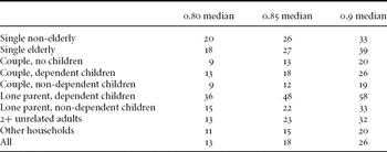
Finally, we look at the headcount rates based on the PI for different household types. These headcounts are based on the relative poverty thresholds (as used in Table 2 above). These show results that are consistent with the literature (Table 3). For example, single elderly households are generally worse off, couples are better off, single parents with dependent children are the worst off of all. These results are what we would expect from our current understanding of the wellbeing of households. Pensioners and lone parents have the lowest standards of living in the UK and tend to live in the worst conditions. Couples with no children are the best off.

TABLE 3.

Headcounts (relative %) by various household types, Model 1, wave 1