

Introduction
Crop diversity, crop rotation and no-tillage or reduced tillage have been identified as management strategies for increasing sustainability of crop production and for increasing economic returns by sustaining crop productivity (Tanaka et al., Reference Tanaka, Lyon, Miller, Merrill, McConkey, Zobeck and Schillinger2010). Increasing crop diversity and reducing tillage can reduce production cost by reducing fuel and labor use, and decreasing use of energy-intensive fertilizers (DeVuyst et al., Reference DeVuyst, Foissey and Kegode2006). However, tradeoffs between machinery costs and fertilizer or pesticide inputs may exist if reducing tillage and crop diversity are not adopted simultaneously (Klemme, Reference Klemme1985; Archer et al., Reference Archer, Pikul and Riedell2002; Zentner et al., Reference Zentner, Wall, Nagy, Smith, Young, Miller, Campbell, McConkey, Brandt, Lafond and Johnston2002a, Reference Zentner, Lafond, Derksen and Campbell2002b). Since the combined impact of crop rotations and no-tillage or reduce tillage practices is variable on crop yields, information regarding the benefits of the system is essential to adopting the combined system.
The key principles in developing a more sustainable agriculture in a dynamic eco-region such as the Northern Great Plains include diversification, flexibility and risk minimization (Thomas and Kevan, Reference Thomas and Kevan1993; Dhuyvetter et al., Reference Dhuyvetter, Thompson, Norwood and Halvorson1996). Diverse cropping systems are consistent with these principles, which have been proposed to minimize the negative socio-economic and environmental impacts of conventional production systems in the region (Zentner et al., Reference Zentner, Campbell, Biederbeck, Miller, Selles and Fernandez2001). However, information on agronomic potential, environmental impacts and economic returns is required to optimize the benefits from diverse cropping systems. Receiving such information is complicated as individual crops interact differently with varying weather conditions and a variety of management factors, such as tillage methods, crop sequencing and cultivar selection, weed and disease control, and nutrient management (Krupinsky et al., Reference Krupinsky, Tanaka, Merrill, Liebig and Hanson2006). Understanding the interaction of crop sequencing and management is essential in creating efficient and profitable systems for crop production while enhancing regeneration and sustainability of soil (Anderson, Reference Anderson2005).
There has been considerable research showing the crop productivity benefits of diverse crop rotations. For example, crop rotations have been shown to increase corn yield from 5 to 30%, soybean yield from 8 to 16% and spring wheat yield from 12 to 35% compared with monoculture (Crookston et al., Reference Crookston, Kurle, Copeland, Ford and Lueschen1991; Copeland et al., Reference Copeland, Allmaras, Crookston and Nelson1993; Lund et al., Reference Lund, Carter and Oplinger1993; West et al., Reference West, Grifith, Steinhardt, Kladivko and Parsons1996; Singer and Cox, Reference Singer and Cox1998; Miller et al., Reference Miller, Waddington, McDonald and Derksen2002). However, despite these findings, crop diversity has tended to decrease over the past 30 yr across the USA (Aguilar et al., Reference Aguilar, Gramig, Hendrickson, Archer, Forcella and Liebig2015). It is important to consider the effect of crop rotation as part of an overall management system that includes the relevant tillage system. No-till and strip-till systems accounted for 39% of the total area for the major crops of corn (Zea mays L.), cotton (Gossypium hirsutum L.), soybeans (Glycine max L.) and wheat in the USA (Wade et al., Reference Wade, Claasen and Wallander2015). Adoption has been higher in the Northern Great Plains, with 49% of the area for these crops produced in a no-till or strip-till system, and even higher in the wheat growing portions of the Northern Great Plains, with 63% of the wheat area in a no-till or strip-till system (Wade et al., Reference Wade, Claasen and Wallander2015).
Historically, in North Dakota, cropping systems were dominated by small grain crops [e.g., wheat, barley (Hordeum vulgare L.), and oat (Avena sativa L.)] and use of fallow, particularly in the more arid western part of the state (Aguilar et al., Reference Aguilar, Gramig, Hendrickson, Archer, Forcella and Liebig2015). As no-till began to be adopted in the 1980s, the associated water conservation benefits allowed producers to crop more intensively and to grow a wider range of crops. In response to increased crop intensity and diversity in the region, Tanaka et al. (Reference Tanaka, Krupinsky, Liebig, Merrill, Ries, Hendrickson, Johnson and Hanson2002) developed an adaptable crop sequencing approach to understand the causal impact of specific management components on crop yields. Referred to as a ‘dynamic cropping system’, Tanaka et al. (Reference Tanaka, Krupinsky, Liebig, Merrill, Ries, Hendrickson, Johnson and Hanson2002) defined it as a ‘long-term strategy of annual crop sequencing that optimizes cropping options and the outcome of production, economics, and resource conservation goals by using sound ecological management principles’ (p. 959). The key components of a dynamic cropping system include crop diversity, adaptability and willingness to take advantage of new opportunities, managing to reduce input costs, use of multiple enterprises to exploit market benefits, environmental awareness to manage resources for future generations and informational awareness to evaluate and apply the best available information (Tanaka et al., Reference Tanaka, Krupinsky, Liebig, Merrill, Ries, Hendrickson, Johnson and Hanson2002). In order to meet these goals, producers need detailed information about factors influencing crop performance. This information provides better recommendations for proper crop sequencing, which is essential for managing successful cropping systems (Krupinsky et al., Reference Krupinsky, Tanaka, Merrill, Liebig and Hanson2006; Kirkegaard et al., Reference Kirkegaard, Christen, Krupinsky and Layzell2008).
The purpose of this research was to evaluate crop productivity and returns for different levels of crop diversity in a long-term, field-scale and no-till cropping system study in the Northern Great Plains. We hypothesized that increased crop diversity would increase crop production, reduce purchased inputs and increase economic returns while reducing economic risks.
Methods and materials
Long-term crop rotation treatments were implemented over time on fields at the Area IV Soil Conservation Districts Cooperative Research Farm located approximately 6 km south of Mandan, North Dakota, USA (46°46′12″N, 100°54′57″W). Crop rotation treatments included: small grain–fallow (SG–Fallow), continuous spring wheat (Cont SW), spring small grain–winter wheat–sunflower (SG–WW–Sun), field pea (Pisum sativum L.)–corn–soybean–spring wheat–winter wheat (Five Year) and a dynamic rotation where crop choices were made annually (Dynamic). Crops in the Dynamic rotation included corn, sunflower, spring wheat, winter wheat, soybean, oat, buckwheat (Fagopyrum esculentum Moench), flax (Linum usitatissimum L.) and alfalfa (Medicago sativa L.). Crops in the Dynamic rotation were selected based on multiple factors including market opportunities and economic returns, soil water and nutrient conditions, pest or disease pressures, and any rotational restriction on herbicide use within each field (Tanaka et al., Reference Tanaka, Krupinsky, Liebig, Merrill, Ries, Hendrickson, Johnson and Hanson2002). The process for selecting crops that were included in the Dynamic rotation each year did not follow a formal set of decision rules, but was based on the judgments and experience of the research team. The management decisions did take into consideration short-term rotational effects identified in previous research (Tanaka et al., Reference Tanaka, Krupinsky, Liebig, Merrill, Ries, Hendrickson, Johnson and Hanson2002, Reference Tanaka, Krupinsky, Merrill, Liebig and Hanson2007; Krupinsky et al., Reference Krupinsky, Tanaka, Merrill, Liebig and Hanson2006), and which have been made available to producers in a computer information product, the Crop Sequence Calculator (Liebig et al., Reference Liebig, Tanaka, Hanson, Archer, Krupinsky, Merrill, Nichols, Hendrickson, Anderson, Charlet and Stott2008).
In rotations with small grains, the small grain phase included spring barley, oat, spring wheat or winter wheat. The SG–Fallow, Cont SW and SW–WW–Sun rotations were established in 1984; Five Year was established in 2009; and Dynamic was established in 2001. The SG–Fallow rotation represents a historical baseline that is no longer commonly used by producers in the area, but has often been used in evaluating cropping system impacts for the region (Halvorson et al., Reference Halvorson, Wienhold and Black2002, Reference Halvorson, Liebig, Archer, West and Tanaka2016; DeVuyst and Halvorson, Reference DeVuyst and Halvorson2004; Liebig et al., Reference Liebig, Tanaka and Wienhold2004). The Cont SW systems represents a more current and more intensive baseline treatment that is low-diversity and is still used in the area. Before 2009, fields included in the Five Year treatment were managed as a dynamic system with crop choices made annually. For the SG–Fallow, Cont SW, SW–WW–Sun and Five Year rotations, each phase of each crop was present every year. For the Dynamic rotation, crops were allocated across ten fields, with at least six different crops included each year. Beginning in 2009, a perennial phase was included in the Dynamic rotation, with one field planted to alfalfa. After 5 yr, the alfalfa was rotated to another field, and the original alfalfa field was returned to annual crop production. The annual land allocation among different crops within the Dynamic rotation is shown in Table 1.
Annual crop area allocation within the dynamic crop rotation (percentage of the total area dynamic rotation area)

Field sizes range from 2 to 20 ha and were predominantly on Temvik and Wilton silt loam soils (USDA: fine-silty, mixed, superactive, frigid Typic and Pachic Haplustolls; FAO: Calcic Siltic Chernozems). However, the Cont SW field differed somewhat from the other treatments and was predominantly on Belfield and Grail clay loam soils (USDA: fine, smectitic, frigid Glossic Natrustolls and Pachic Vertic Argiustolls; FAO: Glossic and Haplic Chernozems). Long-term (98 yr) mean annual precipitation at the site is 412 mm, with 79% of the total received during the growing season (April–September). Long-term mean annual temperature is 4°C, with daily averages fluctuating from <−10°C in the winter to >20°C in the summer. The fields were farmed with field-scale equipment. All treatments were managed as no-till systems. Rotations were not replicated, except for the SG–WW–Sun rotation, which had two replicates. Fertilization and herbicide applications followed practices used by area producers.
Data from 2004 to 2015 were used for this analysis. Yield data were collected from entire fields with all grain from each field weighed using a weigh-wagon. All management operations, and all seed, fertilizer and pesticides were recorded annually for each field. Crop enterprise budgets were constructed for each field based on observed yield and management, using 2014–2015 herbicide (Zollinger et al., Reference Zollinger, Christoffers, Dalley, Endres, Gramig, Howatt, Jenks, Lym, Ostlie, Peters, Robinson, Thostenson and Valenti2016), fertilizer and seed (Swenson and Haugen, Reference Swenson and Haugen2015) and machinery costs (Lazarus, Reference Lazarus2015). Machinery costs included labor, fuel and oil, maintenance and repairs, depreciation, and overhead costs. Machinery overhead costs include interest, insurance and housing costs.
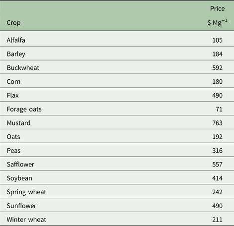
Average annual prices received for North Dakota were used for crop prices (USDA-NASS, 2017), with the exception of buckwheat where crop prices had not been surveyed, so actual prices received were used. Also, North Dakota prices were not available for mustard and safflower in some years, so national average and Montana prices, respectively, were used for these two crops in years when North Dakota prices were not available. In order to separate market effects from production effects, analyses were conducted both using the 2004–2015 annual crop prices and crop prices fixed at the 5-yr average of 2011–2015 annual prices (Table 2).
2011–2015 Average crop prices

Annual net returns for each crop in each field were calculated as:
 $${\rm \pi} _{ijkr} = P_{ij}Y_{ijkr} - C_{ijkr},$$
where π is the net return per hectare; P is the crop price per unit yield; Y is the crop yield per hectare; C is the production cost per hectare; and i is the year, j is the crop, k is the field and r is the rotation. Annual rotation-average net returns were calculated as a weighted average based on the area of each field included in the rotation in that year.
 $${\rm \pi} _{ir} = \; \displaystyle{{\mathop \sum \nolimits_{\,jk} [(P_{ij}Y_{ijkr} - C_{ijkr})]\,A_{ijkr}} \over {\mathop \sum \nolimits_{\,jk} A_{ijkr}}}.$$
Area weighting was used to accommodate the Dynamic treatment, since the area devoted to each crop was part of the management decision process to diversify risk and spread workload over the cropping season. For example, the area devoted to buckwheat, which is a specialty crop, was kept to a small portion of the overall area in most years since it tends to have a higher production risk and a somewhat limited market. Calculating a simple average across crops is not appropriate for the Dynamic system, since the number of crops included in this rotation varied from year to year. For each of the other rotations, approximately equal areas were allocated to each crop in the rotation each year, so area weighted results for these rotations closely match the simple average over the crops included in each rotation. Net returns represent returns to land and management, since no land or management charges are included in the costs. Relative economic risk for each rotation was estimated by the coefficient of variation (CV) of net returns. The risk reward tradeoffs were analyzed by graphing average net returns vs the CV of net returns for each rotation.
Statistical analyses were conducted using mixed models in JMP 13.0, with rotation modeled as a fixed effect, a continuous year variable used to estimate linear time and rotation by time trends, and year as a random effect. A significance level of α = 0.05 was used for statistical tests.
Results and discussion
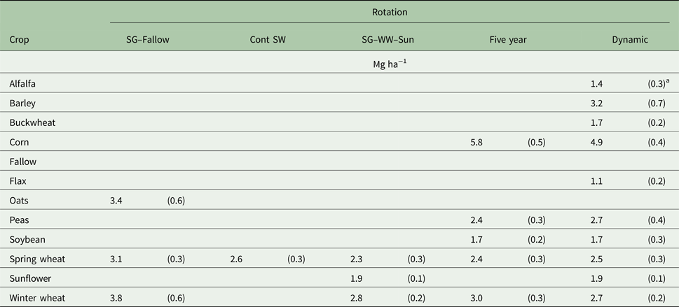
Average crop yields (Table 3), production costs (Table 4) and net returns (Table 5) were estimated for each crop within each crop rotation using the least-squares means output from the statistical model. Different crops had different numbers of observations, particularly in the Dynamic system where some cropping decisions varied annually, so comparisons between crops should be made cautiously. Results for crops with fewer than three observations within a rotation were not reported in Tables 3–5, but were included in calculating rotation average net returns. Overall, buckwheat tended to be the most profitable crop. However, as indicated earlier, it was generally grown on a relatively small area in each year since it is a specialty crop with higher production risk and more limited market. As a specialty crop, it is recognized that not all producers could include buckwheat in their rotations. However, there are several other specialty crops that producers in the area can, and often do, produce on relatively small areas. Other crops that tended to have relatively high net returns were corn, sunflower and alfalfa (Table 5).
Average crop yields within each crop rotation

a Standard errors in parentheses.
Average crop production costs within each crop rotation

a Standard errors in parentheses.
Average crop net returns within each crop rotation, based on 2011–2015 average crop prices

a Standard errors in parentheses.
Spring wheat was included for most years in all crop rotations, so it served as a good crop to benchmark across rotations. Average spring wheat yield was significantly higher for the SG–Fallow rotation than for the other rotations (Table 3), at 3.1 Mg ha−1 compared with 2.6, 2.3, 2.4 and 2.5 Mg ha−1 for Cont SW, SG–WW–Sun, Five Year and Dynamic, respectively. This was expected since fallow was developed as a practice to store additional precipitation for use by the subsequent crop. Although it appeared that spring wheat yields increased over time, the year (P = 0.102) and year by rotation (P = 0.314) trends were not statistically significant due to substantial year-to-year yield variability.
There were no significant differences in spring wheat production costs between rotations (Table 4). However, it should be noted that costs incurred during the fallow year were not included as part of the spring wheat production costs in this analysis. Fallow costs would add $105 ha−1 to spring wheat production costs on average, and these costs were included when comparing the performance of each rotation. There was a significant upward trend in spring wheat production costs across all rotations, with costs increasing by $8 ha−1 yr−1. The cost increases were primarily due to increased fertilizer applications, but also increased pesticide expenditures. There were no significant differences in spring wheat cost trends between rotations.
Average spring wheat net returns were significantly higher for the SG–Fallow rotation than for the other rotations (Table 5), as expected due to higher average yields. However, since costs from the fallow year were not included in this estimate and no income was generated in the fallow year, it is particularly important to look at the rotation average net returns for the SG–Fallow rotation.
Winter wheat was included in most years for the SG–WW–Sun, Five Year and Dynamic rotations. Comparing performance across these rotations, there were no significant differences in average winter wheat yields (Table 3), average winter wheat production costs (Table 4) or average winter wheat net returns (Table 5). There was a significant upward trend in winter wheat production costs across all three of these rotations, with cost increasing by $14 ha−1 yr−1. Similar to spring wheat, the cost increases were primarily due to increases in fertilizer applications. There were no significant differences in winter wheat cost trends between rotations.
Corn was included in most years for the Five Year and Dynamic rotations. Comparing performance between these two rotations, average corn yield was significantly higher for the Five Year rotation than the Dynamic rotation at 5.8 and 4.9 Mg ha−1, respectively (Table 3). However, there were significant year by rotation trend interactions, with corn yield decreasing 0.28 Mg ha−1 yr−1 for the Five Year rotation and increasing 0.16 Mg ha−1 yr−1 for the Dynamic rotation, so that by 2015, trend corn yields were higher for the Dynamic than the Five Year rotation. There were no significant differences between average corn production costs for the Five Year and Dynamic rotations (Table 4). As a result, holding crop prices constant at 2011–2015 levels, average net returns for corn production were higher for the Five Year compared with the Dynamic rotation at $567 and $407 ha−1, respectively (Table 5). But, there were significant year by rotation trend interactions, with net returns for the Five Year rotation decreasing by $51 ha−1 yr−1 and increasing by $26 ha−1 yr−1 for the Dynamic rotation.
Average costs for each rotation are shown in Table 6. Average costs were significantly higher for the SW–WW–Sun than for the Five Year and SG–Fallow rotations. The SG–Fallow rotation had significantly lower annual costs than the other rotations. Average pesticide and fertilizer costs were significantly higher in the SG–WW–Sun rotation than for the other rotations. There were also significant year and year by rotation trends for costs. Costs showed a significant increasing trend over time for the Cont SW and SG–WW–Sun rotations (Table 7). Note that these cost increases were calculated holding input prices constant at 2015 levels, so were not related to input price trends but instead to increasing input use in these rotations. Costs for the Cont SW and SW–WW–Sun rotations increased at $12 ha−1 yr−1 compared with non-significant trends of $4 ha−1 yr−1 for SG–Fallow and Dynamic rotation, and $3 ha−1 yr−1 for the Five Year rotation. These increases in Cont SW and SG–WW–Sun costs were associated primarily with increasing fertilizer applications in these two rotations, increasing at $5 and $6 ha−1 yr−1, respectively. In addition, pesticide expenditures showed significant upward trends for these two rotations at $3 and $2 ha−1 yr−1, respectively. Increasing costs in these two systems are indicative of the challenges in maintaining crop productivity in less-diverse crop rotations.
Rotation average gross returns, costs and net returns, 2004–2015 average

a Values within a row followed by a different letter are significantly different at P ≤ 0.05.
Rotation average trends in gross returns, costs and net returns, 2004–2015

* P-value in parentheses.
Rotation average gross returns were significantly lower for SG–Fallow than for any of the other rotations based on either 2011–2015 average crop prices or annual crop prices (Table 6). Numerically, gross return rankings were Dynamic > Five Year > SG–WW–Sun > SG–Fallow. Rotation average net returns were also significantly lower for SG–Fallow than for the other rotations. Based on 2011–2015 average crop prices, numerical net returns rankings were Five Year > Dynamic > SG–WW–Sun > SG–Fallow. Year and year by rotation trends were not significant for either gross returns or net returns. Holding crop prices fixed at 2011–2105 averages, net return trend estimates indicated potential separation between more diverse rotations (Dynamic and Five Year) compared with less diverse rotations (SG–WW–Sun, Cont SW and SG–Fallow), with returns for the more diverse rotations increasing at a faster rate (Table 7). These potential trends warrant further monitoring of these systems over more years to see if significant trends emerge.
Diversification is a method often used to reduce risk. Diverifying rotations can be effective in reducing risks that occur due to both price and yield variability if producers are able to select crops that have prices or yields that are not highly correlated. However, there can potentially be tradeoffs between reducing risk and reducing returns. When net returns were calculated using annual prices, increasing crop diversity generally increased average net returns and reduced relative risks (Fig. 1). While the SG–WW–Sun rotation had slightly lower relative risk than the Five Year rotation, the Five Year rotation had higher average net returns. The Dynamic rotation resulted in the higest net returns and lowest relative risk when faced with both price and yield risks. When returns were calculated using 2011–2015 average crop prices, the Five Year rotation had slightly higher average net returns than the Dynamic rotation, but also had higher relative risk (Fig. 1). These results indicate that more diverse rotations were effective at reducing relative risks associated with yield variability. However, the Dynamic rotation might not achieve the highest level of returns when market (price) risks were not included. This was not surprising since part of the criteria used in selecting the crops grown in the Dynamic rotation each year were crop price expectations for that year. This approach would not be anticipated to be as effective at maximizing net returns when evaluated at fixed price levels that may differ substantially from the targeted prices expectations. Even though the process for selecting crops included in the Dynamic rotation each year was not formalized and was based on the judgments and experience of the research team, these results indicate that the selection process was generally effective at both increasing net returns and reducing relative risk. A question with the Dynamic rotation is the effect of the alfalfa perennial crop on these results. Another question is the effect of the buckwheat specialty crop on these results. To answer these questions, we looked at the results using 2011–2015 annual prices, but excluding the net returns from the fields and years when alfalfa was grown and, alternatively, excluding buckwheat in years when buckwheat was grown. The results in both cases changed only slightly, with average net returns decreasing to $291 and $292 ha−1, respectively, when alfalfa or buckwheat were excluded. The CV increased to 0.56. and 0.59, respectively, when alfalfa or buckwheat were excluded. So, even without alfalfa production or without buckwheat production, the Dynamic rotation had the lowest relative risk, and was only slightly less profitable than the Five Year rotation.
Tradeoffs between average net returns and relative economic risk (CV of net returns), calculated with annual crop prices and with 2011–2015 average crop prices.

Looking at the near-surface soil conditions (0–10 cm) in this same field study, Liebig et al. (Reference Liebig, Archer and Tanaka2014) found that the more diverse rotations (Five Year and Dynamic) had higher levels of soil organic carbon (SOC) in 2012 than the less diverse rotations, and that these were the only treatments in which SOC levels had increased between 1983 and 2012. Cont SW was not included in that analysis, since that system was on a different soil type. However, we include the results for Cont SW here for completeness. In comparing SOC changes with net returns in these systems (Fig. 2), results suggest that by selecting diverse rotations in a no-till sytem, producers in this region may be able to simultaneously realize economic benefits while maintaining or building SOC. However, highest SOC increases were seen with Cont SW, but net returns were lower with this system than with more diverse systems, indicating a potential tradeoff in achieving both goals of increasing SOC and net returns.
Tradeoffs between average net returns and annual change in SOC. Net returns calculated with 2011–2015 average crop prices.

Conclusions
Comparing long-term performance of rotations with differing levels of crop diversity, crop productivity, as measured by gross returns, increased significantly when moving from a SG–Fallow rotation to more intensive and diverse rotations. While further increases in crop diversity appeared to further increase productivity, the effects were not statistically significant. Production costs were significantly lower for the least productive SG–Fallow rotation. Production costs were numerically higher for the Cont SW and SG–WW–Sun rotations than for the Five Year and Dynamic rotations indicating some benefits to diversifying crop rotations in reducing input use and production costs; however, the differences were not statistically significant. Somewhat surprisingly, input use as reflected in production costs showed an upward trend for all but the Five Year rotation. This upward trend was significantly positive and higher for the Cont SW and SG–WW–Sun rotations raising concerns about the long-term sustainability of these rotations. Diversifying to a Five Year rotation provided some evidence suggesting that a more diverse rotation could reduce the need for purchased inputs in the long-term. While there was some evidence of production increases over time with potentially more rapid increases in more diverse systems, these differences were not statistically significant. This highlights the difficulty in quantifying long-term system effects on long-term productivity in regions where year-to-year variability in crop production is high. Moving from the SG–Fallow to more intensive and diverse rotations significantly increased net returns. Further increases in crop diversity maintained and possibly increased net returns. Increasing crop diversity also showed benefits in reducing relative economic risk, indicating that these systems would be economically beneficial to producers while maintaining crop productivity, building or maintaining SOC, and, in some cases, reducing input use.
Acknowledgements
The authors acknowledge the contribution of the Area IV SCD in North Dakota for providing the land to conduct research reported in this paper. They also acknowledge Marvin Hatzenbuhler who managed the cropping system treatments, Robert Kolberg who assisted with field management and compiled management records, Delmer Schlenker who assisted with field management, and many field and laboratory support personnel who have invested countless hours to maintain plots and collect data on the Area IV SCD Research Farm since its inception. The US Department of Agriculture, Agricultural Research Service, is an equal opportunity/affirmative action employer and all agency services are available without discrimination. Mention of commercial products and organizations in this paper is solely to provide specific information. It does not constitute endorsement by USDA-ARS over other products and organizations not mentioned.