2.1 Reduced-order aerodynamic modeling in transonic buffeting flows

This subsection presents a state-space-based ROM to capture the linear and nonlinear characteristics of transonic unsteady aerodynamic forces accurately. The structure of the modified nonlinear ROM is defined as the following state equations in a vector form

(1) \begin{align}\begin{array}{l}{{\boldsymbol{x}}_a}\left( {k + 1} \right) = {{\boldsymbol{A}}_a}{{\boldsymbol{x}}_a}(k) + {{\boldsymbol{B}}_a}{\boldsymbol{u}}(k) + {{\boldsymbol{E}}_a}{\boldsymbol{\varPhi }}\left( {{\rm{diag}}\left( {{{\boldsymbol{x}}_0}} \right){{\boldsymbol{x}}_a}(k)} \right) + {{\boldsymbol{F}}_a}{\boldsymbol{\varPhi }}\left( {{\rm{diag}}\left( {{{\boldsymbol{u}}_0}} \right){\boldsymbol{u}}(k)} \right)\\[6pt]{{\boldsymbol{y}}_a}(k) = {{\boldsymbol{C}}_a}{{\boldsymbol{x}}_a}(k) + {{\boldsymbol{D}}_a}{\boldsymbol{u}}(k) + {{\boldsymbol{G}}_a}{\boldsymbol{\varPhi }}\left( {{\rm{diag}}\left( {{{\boldsymbol{x}}_0}} \right){{\boldsymbol{x}}_a}(k)} \right) + {{\boldsymbol{H}}_a}{\boldsymbol{\varPhi }}\left( {{\rm{diag}}\left( {{{\boldsymbol{u}}_0}} \right){\boldsymbol{u}}(k)} \right)\end{array}\end{align}

where ${{\boldsymbol{x}}_a} \in {\mathbb{R}^n}$ , ${\boldsymbol{u}} \in {\mathbb{R}^p}$ and ${{\boldsymbol{y}}_a} \in {\mathbb{R}^q}$ are the state vector, the input vector, and the output vector, respectively. In this paper, the displacements are used as the input vector ${\boldsymbol{u}}$ and the aerodynamic forces are used as the output vector ${{\boldsymbol{y}}_a}$ . The influences of various time derivatives of the displacements on the aerodynamic forces are implicitly captured within the state-space model. Therefore, these derivative terms do not need to be explicitly included in the inputs. The coefficient matrices $\left( {{{\boldsymbol{A}}_a},{{\boldsymbol{B}}_a},{{\boldsymbol{C}}_a},{{\boldsymbol{D}}_a}} \right)$ of the linear part in Equation (1) are constants to be identified via the eigensystem realisation algorithm (ERA), and the coefficients matrices $\left( {{{\boldsymbol{E}}_a},\ {{\boldsymbol{F}}_a},\ {{\boldsymbol{G}}_a},\ {{\boldsymbol{H}}_a}} \right)$ of the nonlinear part are constants to be determined via the Levenberg-Marquardt (LM) algorithm [Reference Moré31]. Here, $ \boldsymbol{\varPhi}({\cdot})$ is the vector of nonlinear mapping with the entries assumed as a hyperbolicsine function $\sinh \left( \cdot \right)$ so as to accurately model the complex transonic aerodynamic forces due to different amplitudes of structural vibrations and buffeting flows. As the hyperbolicsine function $\sinh \left( \cdot \right)$ is a strictly increasing function, the scale factors ${{\boldsymbol{x}}_0}$ and ${{\boldsymbol{u}}_0}$ are identified in the optimisation produce for the state vector and the input vector to properly describe nonlinearities.

According to the structure of Equation (1), the identification process of the above nonlinear ROM can be constructed as shown in Fig. 1, where the parameters of the linear model are respectively identified and selected via the impulsive signal and the sinusoidal signal generated via CFD codes first, and then are kept as constants while the parameters of the nonlinear part are determined via the filtered white Gaussian noise (FWGN) signal produced via CFD.

Figure 1.

Flow chart of identification of a nonlinear ROM.

To construct the nonlinear ROM in Equation (1), the first stage is to identify the coefficient matrices ${{\boldsymbol{A}}_a}$ , ${{\boldsymbol{B}}_a}$ , ${{\boldsymbol{C}}_a}$ and ${{\boldsymbol{D}}_a}$ in the linear ROM via ERA. For this purpose, the discrete-time impulsive and sinusoidal response signals generated via CFD are used as the training and validation signals, respectively. The detailed identification procedure can be found in Ref. [Reference Yang, Huang, Liu, Zhao and Hu32].

After the above matrices of the linear part are estimated, the next step is to keep the matrices unchanged and use the LM algorithm to determine the optimised parameters in the nonlinear part. The entries in matrices ${{\boldsymbol{x}}_0}$ , ${{\boldsymbol{u}}_0}$ , ${{\boldsymbol{E}}_a}$ , ${{\boldsymbol{F}}_a}$ , ${{\boldsymbol{G}}_a}$ and ${{\boldsymbol{H}}_a}$ can be collected as an unknown vector ${\boldsymbol{p}}$ of dimension $\left( {n + p} \right) \times \left( {n + q} \right){\rm{ + }}p + q$ . Subsequently, the following ordinary differential equations corresponding to vector ${\boldsymbol{p}}$ should be solved until the output error ${{\boldsymbol{e}}_k} = {{\boldsymbol{y}}_{{\rm{CFD}}}}(k) - {{\boldsymbol{y}}_a}\left( {k;\ {\boldsymbol{p}}} \right)$ is small enough. That is, vector ${\boldsymbol{p}}$ yields

(2) \begin{align}\begin{array}{l}{\boldsymbol{x}}_a^{k + 1} = {{\boldsymbol{A}}_a}{\boldsymbol{x}}_a^k + {{\boldsymbol{B}}_a}{{\boldsymbol{u}}^k} + {{\boldsymbol{E}}_a}{\boldsymbol{\varPhi }}\left( {{{\boldsymbol{x}}_0},{\boldsymbol{x}}_a^k} \right) + {{\boldsymbol{F}}_a}{\boldsymbol{\varPhi }}\left( {{{\boldsymbol{u}}_0},{{\boldsymbol{u}}^k}} \right)\\[6pt]{\boldsymbol{x}}_{a/{\boldsymbol{p}}}^{k + 1} = {{\boldsymbol{A}}_a}{\boldsymbol{x}}_{a/{\boldsymbol{p}}}^k + {{\boldsymbol{E}}_{a/{\boldsymbol{p}}}}{\boldsymbol{\varPhi }}\left( {{{\boldsymbol{x}}_0},{\boldsymbol{x}}_a^k} \right) + {{\boldsymbol{E}}_a}{\boldsymbol{\varPhi }}{\left( {{{\boldsymbol{x}}_0},{\boldsymbol{x}}_a^k} \right)_{/{\boldsymbol{p}}}} + {{\boldsymbol{F}}_{a/{\boldsymbol{p}}}}{\boldsymbol{\varPhi }}\left( {{{\boldsymbol{u}}_0},{{\boldsymbol{u}}^k}} \right) + {{\boldsymbol{F}}_a}{\boldsymbol{\varPhi }}{\left( {{{\boldsymbol{u}}_0},{{\boldsymbol{u}}^k}} \right)_{/{\boldsymbol{p}}}}\\[6pt]{\boldsymbol{y}}_a^k = {{\boldsymbol{C}}_a}{\boldsymbol{x}}_a^k + {{\boldsymbol{D}}_a}{{\boldsymbol{u}}^k} + {{\boldsymbol{G}}_a}{\boldsymbol{\varPhi }}\left( {{{\boldsymbol{x}}_0},{\boldsymbol{x}}_a^k} \right) + {{\boldsymbol{H}}_a}{\boldsymbol{\varPhi }}\left( {{{\boldsymbol{u}}_0},{{\boldsymbol{u}}^k}} \right)\\[6pt]{\boldsymbol{y}}_{a/{\boldsymbol{p}}}^k = {{\boldsymbol{C}}_a}{\boldsymbol{x}}_{a/{\boldsymbol{p}}}^k + {{\boldsymbol{G}}_{a/{\boldsymbol{p}}}}{\boldsymbol{\varPhi }}\left( {{{\boldsymbol{x}}_0},{\boldsymbol{x}}_a^k} \right) + {{\boldsymbol{G}}_a}{\boldsymbol{\varPhi }}{\left( {{{\boldsymbol{x}}_0},{\boldsymbol{x}}_a^k} \right)_{/{\boldsymbol{p}}}} + {{\boldsymbol{H}}_{a/{\boldsymbol{p}}}}{\boldsymbol{\varPhi }}\left( {{{\boldsymbol{u}}_0},{{\boldsymbol{u}}^k}} \right) + {{\boldsymbol{H}}_a}{\boldsymbol{\varPhi }}{\left( {{{\boldsymbol{u}}_0},{{\boldsymbol{u}}^k}} \right)_{/{\boldsymbol{p}}}}\end{array}\end{align}

where

(3) \begin{align}\begin{array}{l}{{\boldsymbol{\chi }}_{/{\boldsymbol{p}}}} = \dfrac{{\partial {\boldsymbol{\chi }}}}{{\partial {\boldsymbol{p}}}},{\rm{ }}\quad {\boldsymbol{\chi }} = {{\boldsymbol{x}}_a},{{\boldsymbol{y}}_a},{{\boldsymbol{E}}_a},{{\boldsymbol{F}}_a},{{\boldsymbol{G}}_a},{{\boldsymbol{H}}_a},{\boldsymbol{\varPhi }}\\[6pt]{\boldsymbol{\varPhi }}{\left( {{{\boldsymbol{\delta }}_0},{\boldsymbol{\delta }}} \right)_{/{\boldsymbol{p}}}} = \dfrac{{\partial {\boldsymbol{\varPhi }}\left( {{{\boldsymbol{\delta }}_0},{\boldsymbol{\delta }}} \right)}}{{\partial {{\boldsymbol{\delta }}_0}}}\dfrac{{\partial {{\boldsymbol{\delta }}_0}}}{{\partial {\boldsymbol{p}}}} + \dfrac{{\partial {\boldsymbol{\varPhi }}\left( {{{\boldsymbol{\delta }}_0},{\boldsymbol{\delta }}} \right)}}{{\partial {\boldsymbol{\delta }}}}\dfrac{{\partial {\boldsymbol{\delta }}}}{{\partial {\boldsymbol{p}}}},{\rm{ }}{\boldsymbol{\delta }} = {\boldsymbol{x}},{\boldsymbol{u}}\end{array}\end{align}

The unknown vector ${\boldsymbol{p}}$ is updated at each iteration via the following least-square problem [Reference Mannarino and Dowell33]

(4) \begin{align}\left( {{{\boldsymbol{J}}^{\rm{T}}}{\boldsymbol{J}} + \lambda {\boldsymbol{I}}} \right)\Delta {\boldsymbol{p}} = - {{\boldsymbol{J}}^{\rm{T}}}{\boldsymbol{e}}\end{align}

where $\lambda $ is a regularisation parameter used to keep the left-hand-side matrix always nonsingular. The expansions of vectors in Equation (4) are evaluated as

(5) \begin{align}{\boldsymbol{e}} = \left\{ {\left. {\begin{array}{*{20}{c}}{{{\boldsymbol{e}}_1}}\\{{{\boldsymbol{e}}_2}}\\ \vdots \\{{{\boldsymbol{e}}_m}}\end{array}} \right\}} \right.,\quad {\boldsymbol{J}} = \left[ {\begin{array}{*{20}{c}}{{{\boldsymbol{e}}_{1/p}}}\\{{{\boldsymbol{e}}_{2/p}}}\\ \vdots \\{{{\boldsymbol{e}}_{m/p}}}\end{array}} \right] = - \left[ {\begin{array}{*{20}{c}}{{{\boldsymbol{y}}_{a/p}}\left( 1 \right)}\\{{{\boldsymbol{y}}_{a/p}}\left( 2 \right)}\\ \vdots \\{{{\boldsymbol{y}}_{a/p}}\left( m \right)}\end{array}} \right]\end{align}

The iteration stops when either the Euclidean norm of the output error ${\left\| {\boldsymbol{e}} \right\|_2}$ achieves a sufficiently small value or the variation between two iterations is smaller than a user-defined threshold.

2.2 Nonlinear aeroservoelastic modeling

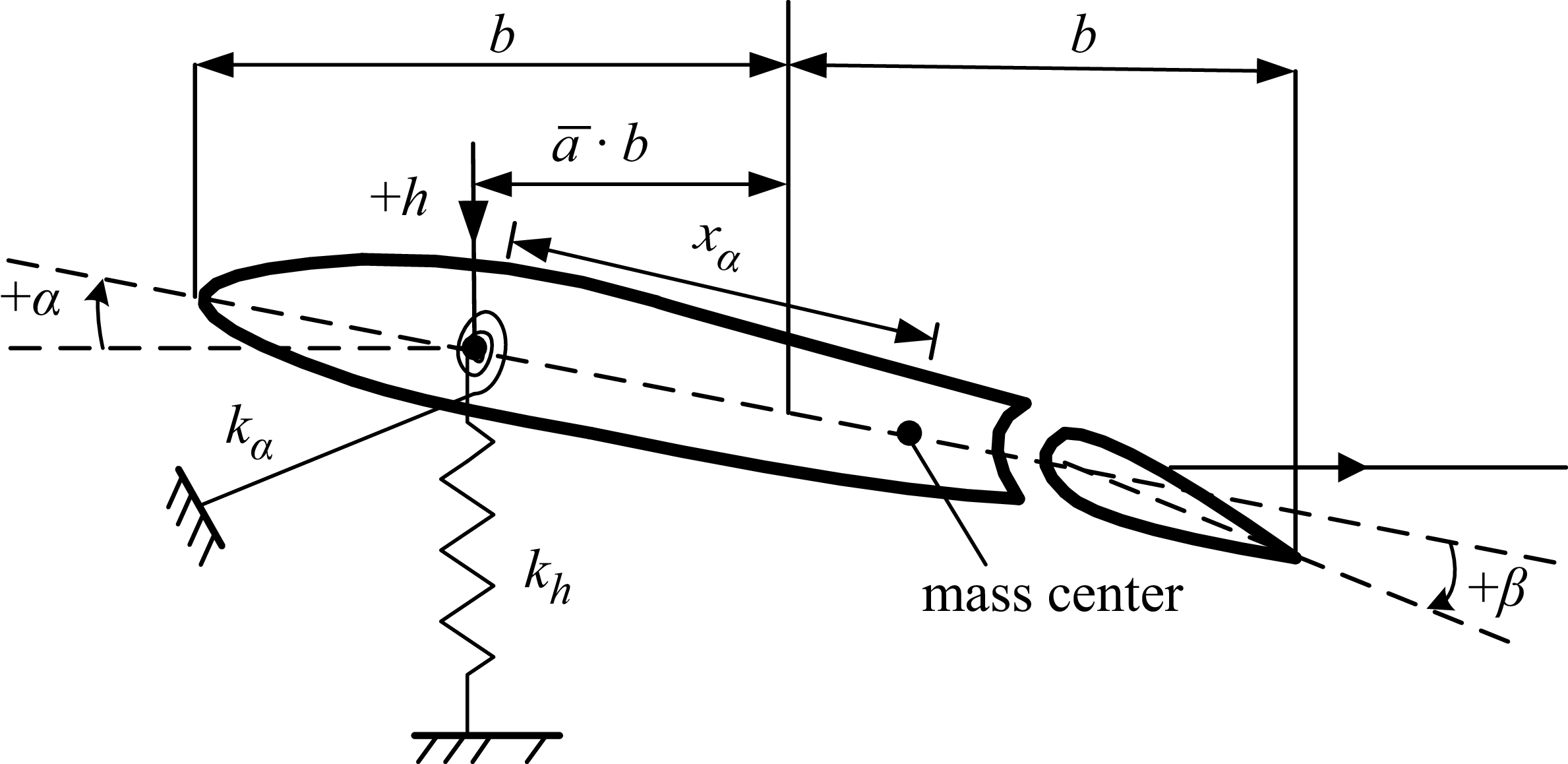
This subsection deals with the dynamic modeling for a two-dimensional aerofoil system having a control surface shown in Fig. 2. The aerofoil system has three degrees of freedom, that is, the plunge, the pitch and the control surface motion, and the mean angle-of-attack is zero. The three-degree-of-freedom dynamic equations of NACA0012 aerofoil were established in Ref. [Reference Theodorsen34] and subsequently simplified in Ref. [Reference Waszak35] based on the assumption of sufficiently large stiffness for the control surface degree of freedom. The dynamic equations in this paper are also derived from this assumption, and the motion of the control surface is assumed to be unaffected by aerodynamic forces and inertial coupling with other degrees of freedom. With the help of the Lagrange equation of the second kind and the dimensionless structural time $\tau = {\omega _\alpha }t$ , it is easy to establish the dynamic equation of the aerofoil as follows

(6) \begin{align}\boldsymbol{M} \boldsymbol{\ddot{\xi}} + \boldsymbol{K} \boldsymbol{\xi } = \boldsymbol{S} \ddot \beta + \boldsymbol{f} \end{align}

Figure 2.

Aerofoil system with a control surface.

The vectors and matrices in Equation (6) read

(7) \begin{align} \boldsymbol{M} & = \left[ \begin{array}{c@{\quad}c} 1 & {{{\bar x}_\alpha }} \\[6pt] {{{\bar x}_\alpha }} & {\bar r_\alpha ^2} \end{array} \right],\quad \boldsymbol{K} = \left[ \begin{array}{c@{\quad}c} {{{\left( {{\omega _h}/{\omega _\alpha }} \right)}^2}} & 0 \\[6pt] 0 & {\bar r_\alpha ^2} \end{array} \right],\quad {\boldsymbol{\xi }} = \left\{ \begin{array}{l} {{\xi _1}} \\ {{\xi _2}} \end{array} \right\} = \left\{ \begin{array}{l} {h/b} \\ \alpha \end{array}\right\},\ \boldsymbol{S} = - \left\{ \begin{array}{l} {{{\bar S}_{h\beta }}} \\ {{{\bar S}_{\alpha \beta }}} \end{array} \right\},\nonumber\\[6pt]\boldsymbol{f} & = {{{{\left( {V_\infty ^ * } \right)}^2}} \over \pi } \left\{ \begin{array}{l} { - {C_l}} \\ {2{C_m}} \end{array} \right\} \end{align}

where ${\bar x_\alpha }$ represents the static unbalance of the aerofoil, which is the dimensionless distance between the mass centre and the stiffness centre, ${\bar r_\alpha }$ is the gyration radius of the aerofoil around the elastic axis ${\omega _h}$ and ${\omega _\alpha }$ are the natural frequencies of the plunge and pitch, respectively. $b$ is the half-chord length, and $V_\infty ^ * = {V_\infty }/\left( {{\omega _\alpha }b\sqrt \mu } \right)$ represents the reduced velocity. ${V_\infty }$ denotes the free-stream velocity, and $\mu = m/\pi {\rho _\infty }{b^2}$ denotes the mass ratio. ${\bar S_{h\beta }}$ is the dimensionless inertial coupling between the plunge and the control surface motion, and ${\bar S_{\alpha \beta }}$ is the dimensionless inertial coupling between the pitch and the control surface motion. The lift coefficient ${C_l}$ and the moment coefficient ${C_m}$ are the entries in the output vector ${{\boldsymbol{y}}_a}$ in Section 2.1. Therefore, the inputs to the reduced-order aerodynamic model are plunge, pitch and control surface motion, while the outputs are lift coefficient and moment coefficient.

In general, the deflection angle of the control surface cannot respond to a control input instantaneously. Therefore, the dynamic model of the control surface under actuation is expressed as

(8) \begin{align}\ddot \beta + 2{\omega _\beta }{\zeta _\beta }\dot \beta + \omega _\beta ^2\beta = {k_\beta }\omega _\beta ^2{\beta _c}\end{align}

where ${k_\beta }$ , ${\zeta _\beta }$ , ${\omega _\beta }$ , and ${\beta _c}$ are the input gain, the damping ratio, the natural frequency and the control command, respectively. By combining Equations (6), (7) and (8), the dynamic model of the two-dimensional aerofoil system with a control surface is formulated as

(9) \begin{align}\dot{\boldsymbol{x}}_{s} = {{\boldsymbol{A}}_s}{{\boldsymbol{x}}_s} + {{\boldsymbol{B}}_c}{\beta _c} + {{\boldsymbol{B}}_q}\kern2pt{\boldsymbol{f}}\end{align}

where the vectors and matrices are defined as

(10) \begin{align} {\boldsymbol{A}_{\boldsymbol{s}}} & = \left[ \begin{array}{c@{\quad}c} {{{\boldsymbol{0}}_{3 \times 3}}} & {{\boldsymbol{I}_3}} \\[6pt] { - {\boldsymbol{M}_s}^{ - 1}{\boldsymbol{K}_s}} & { - {\boldsymbol{M}_s}^{ - 1}{\boldsymbol{C}_s}}\end{array}\right]{\boldsymbol{, }}\quad {\boldsymbol{B}_{\boldsymbol{c}}}=\left[ \begin{array}{c} {{{\boldsymbol{0}}_{3 \times 1}}} \\[6pt] { - {\boldsymbol{M}_s}^{{\rm{ - 1}}}{\tilde{\boldsymbol{B}}}} \end{array} \right]{\boldsymbol{, }}\quad {\boldsymbol{B}_{\boldsymbol{q}}}=\left[ \begin{array}{c} {{{\boldsymbol{0}}_{3 \times 2}}} \\[6pt] {{\boldsymbol{M}_s}^{{\rm{ - 1}}}\left[ {{\boldsymbol{I}_{\rm{2}}};\ {{\boldsymbol{0}}_{{\rm{1}} \times {\rm{2}}}}} \right]} \end{array} \right], \nonumber \\[8pt] {\boldsymbol{x}_s} & = {\left[ \begin{array}{c@{\quad}c@{\quad}c@{\quad}c@{\quad}c@{\quad}c} {{\xi _1}} & {{\xi _2}} & \beta & {{{\dot \xi }_1}} & {{{\dot \xi }_2}} & {\dot \beta }\end{array} \right]^T} \end{align}

The definitions of matrices ${{\boldsymbol{M}}_s}$ , ${{\boldsymbol{C}}_s}$ , ${{\boldsymbol{K}}_s}$ and $\tilde{\boldsymbol{B}}$ are, respectively, given as

(11) \begin{align}\begin{array}{l}{{\boldsymbol{M}}_s} = \left[ {\begin{array}{c@{\quad}c@{\quad}c}1 & {}{{{\bar x}_\alpha }} & {}0\\[5pt]{{{\bar x}_\alpha }} & {}{\bar r_\alpha ^2} & {}0\\[5pt]0 & {}0 {}& 1\end{array}} \right],\ {{\boldsymbol{C}}_s} = \left[ {\begin{array}{c@{\quad}c@{\quad}c}0 & {}0 & {}{ - 2{\omega _\beta }{\zeta _\beta }{{\bar S}_{h\beta }}}\\[5pt]0 & {}0 & {}{ - 2{\omega _\beta }{\zeta _\beta }{{\bar S}_{\alpha \beta }}}\\[5pt]0 & {}0 & {}{2{\zeta _\beta }{\omega _\beta }}\end{array}} \right],{\rm{ }}\\[24pt] {{\boldsymbol{K}}_s} = \left[ {\begin{array}{c@{\quad}c@{\quad}c}{{{\left( {{\omega _h}/{\omega _\alpha }} \right)}^2}} & {}0 & {}{ - \omega _\beta ^2{{\bar S}_{h\beta }}}\\[5pt]0 & {}{\bar r_\alpha ^2} & {}{ - \omega _\beta ^2{{\bar S}_{\alpha \beta }}}\\[5pt]0 & {}0 & {}{\omega _\beta ^2}\end{array}} \right],\ {\boldsymbol{\tilde B}} = \left\{ {\begin{array}{c}{{k_\beta }\omega _\beta ^2{{\bar S}_{h\beta }}}\\[5pt]{{k_\beta }\omega _\beta ^2{{\bar S}_{h\beta }}}\\[5pt]{{k_\beta }\omega _\beta ^2}\end{array}} \right\}\end{array}\end{align}

To design the control law and analyse the aerofoil system under control, the structure accelerations are used as the feedback signals. The output equation of the controlled aerofoil system reads

(12) \begin{align}{y_s} = \left[ {\begin{array}{c@{\quad}c}b & {}{{x_c}}\end{array}} \right]\left[ {\begin{array}{c@{\quad}c@{\quad}c}{{{\boldsymbol{0}}_{2 \times 3}}} & {}{{{\boldsymbol{I}}_2}} & {}{{{\boldsymbol{0}}_{2 \times 1}}}\end{array}} \right]{{\dot{\boldsymbol{x}}}_s}\end{align}

where ${x_c}$ is the distance between the accelerometer and the elastic axis, ${y_s}$ is the acceleration signal used to analyse the controlled aerofoil system.

To establish the ASE model, the dynamic model needs to be rebuilt in the discrete-time step as follows

(13) \begin{align} {{\boldsymbol{x}}_s}\left( {k + 1} \right) & = {\boldsymbol{A}}_s^d{{\boldsymbol{x}}_s}(k) + \boldsymbol{B}_c^d{\beta _c}(k) + \boldsymbol{B}_q^d\kern1.5pt{\boldsymbol{f}}(k) \nonumber \\[6pt]{y_s}(k) & = \left[ {\begin{array}{c@{\quad}c}b & {}{{x_c}}\end{array}} \right]\left[ {\begin{array}{c@{\quad}c@{\quad}c}{{{\boldsymbol{0}}_{2 \times 3}}} & {}{{{\boldsymbol{I}}_2}} & {}{{{\boldsymbol{0}}_{2 \times 1}}}\end{array}} \right]{{{\dot{\boldsymbol{x}}}}_s}(k) \nonumber \\[6pt]& = \left[ {\begin{array}{c@{\quad}c}b & {}{{x_c}}\end{array}} \right]\left[ {\begin{array}{c@{\quad}c@{\quad}c}{{{\boldsymbol{0}}_{2 \times 3}}} & {}{{{\boldsymbol{I}}_2}} & {}{{{\boldsymbol{0}}_{2 \times 1}}}\end{array}} \right]\left( {{{\boldsymbol{A}}_s}{{\boldsymbol{x}}_s}(k) + {{\boldsymbol{B}}_c}{\beta _c}(k) + {{\boldsymbol{B}}_q}\kern1.5pt{\boldsymbol{f}}(k)} \right) \end{align}

where ${\boldsymbol{A}}_s^d$ , ${\boldsymbol{B}}_c^d$ and ${\boldsymbol{B}}_q^d$ are the matrices corresponding to the discrete dynamic model. The final discrete equations of the reduced-order ASE system can be formulated as

(14) \begin{align} & {\boldsymbol{x}_a}\left( {k + 1} \right) = {\boldsymbol{A}_a}{\boldsymbol{x}_a}(k) + {\boldsymbol{B}_a}\boldsymbol{u}(k) + {\boldsymbol{E}_a}{\boldsymbol{\varPhi }}\left( {{\rm{diag}}\left( {{\boldsymbol{x}_0}} \right){\boldsymbol{x}_a}(k)} \right) + {\boldsymbol{F}_a}{\boldsymbol{\varPhi }}\left( {{\rm{diag}}\left( {{\boldsymbol{u}_0}} \right)\boldsymbol{u}(k)} \right) \nonumber \\[6pt] & {\boldsymbol{y}_a}(k) = {\boldsymbol{C}_a}{\boldsymbol{x}_a}(k) + {\boldsymbol{D}_a}\boldsymbol{u}(k) + {\boldsymbol{G}_a}{\boldsymbol{\varPhi }}\left( {{\rm{diag}}\left( {{\boldsymbol{x}_0}} \right){\boldsymbol{x}_a}(k)} \right) + {\boldsymbol{H}_a}{\boldsymbol{\varPhi }}\left( {{\rm{diag}}\left( {{\boldsymbol{u}_0}} \right)\boldsymbol{u}(k)} \right) \nonumber\\[6pt] & {\boldsymbol{x}_s}\left( {k + 1} \right) = \boldsymbol{A}_s^d{\boldsymbol{x}_s}(k)+ \boldsymbol{B}_c^d{\beta _c}(k)+ \boldsymbol{B}_q^d\kern1.5pt\boldsymbol{f}(k) \\[6pt] & {y_s}(k) = \left[ \begin{array}{l@{\quad}l} b & {{x_c}} \end{array} \right]\left[ \begin{array}{l@{\quad}l@{\quad}l} {{{\boldsymbol{0}}_{2 \times 3}}} & {{\boldsymbol{I}_2}} & {{{\boldsymbol{0}}_{2 \times 1}}}\end{array} \right]\left( {{\boldsymbol{A}_s}{\boldsymbol{x}_s}(k)+{\boldsymbol{B}_c}{\beta _c}(k)+{\boldsymbol{B}_q}\kern1.5pt\boldsymbol{f}(k)} \right) \nonumber\\[6pt] & \boldsymbol{u}(k)=\left[ \begin{array}{l@{\quad}l} {{{\boldsymbol{1}}_{3 \times 1}}} & {{{\boldsymbol{0}}_{3 \times 1}}} \end{array} \right]{\boldsymbol{x}_s}(k),\ \boldsymbol{f}(k)= = {{{{\left( {V_\infty ^ * } \right)}^2}} \over \pi }{\boldsymbol{y}_a}(k) \nonumber \end{align}

To improve the accuracy of aeroelastic response prediction, the predictor/corrector scheme [Reference Edwards, Bennett, Whitlow and Seidel36] can be used in Equation (14).

3.1 Design of the linear extended state observer

It is well known that the linearised mathematical model of a single-input/single-output (SISO) ASE system can be expressed in the form of a transfer function as

(15) \begin{align}\frac{{{y_s}(s)}}{{{\beta _c}(s)}} = \frac{{{b_r}{s^r} + \cdots + {b_{n + 1}}{s^{n + 1}} + {b_n}{s^n} + {b_{n - 1}}{s^{n - 1}} + \cdots + {b_1}s + {b_0}}}{{{a_r}{s^r} + \cdots + {a_{n + 1}}{s^{n + 1}} + {s^n} + {a_{n - 1}}{s^{n - 1}} + \cdots + {a_1}s + {a_0}}},\quad r \geq n\end{align}

where ${a_i}$ and ${b_i},i = 1,2 \cdots r$ are the unknown coefficients. However, the ASE system is nonlinear due to the nonlinearity and instability of the aerodynamic forces. The nonlinear ASE system can be rewritten in the time domain as

(16) \begin{align} y_s^{\left( n \right)} = f\left( {{y_s},{{\dot y}_s}, \cdots ,y_s^{(n - 1)},y_s^{(n + 1)} \cdots ,y_s^{(r)},{{\dot \beta }_c}, \cdots \beta _c^{(n)},\beta _c^{(n + 1)}, \cdots \beta _c^{(r)},w,t} \right) + {b_0}{\beta _c} \end{align}

where $w$ is the output noise and $f$ is the sum of the unknown disturbances, including not only the external disturbances but also the internal structure uncertainties. If the exact value ${b_0}$ is not available, the estimated value ${\bar b_0}$ should be introduced to design the control system, and Equation (16) can be recast as

(17) \begin{align}y_s^{\left( n \right)} = \bar f + {\bar b_0}{\beta _c}\end{align}

where

(18) \begin{align}\bar f = f\left( {{y_s},{{\dot y}_s}, \cdots ,y_s^{(n - 1)},y_s^{(n + 1)} \cdots ,y_s^{(r)},{{\dot \beta }_c}, \cdots \beta _c^{(n)},\beta _c^{(n + 1)}, \cdots \beta _c^{(r)},w,t} \right){\rm{ + }}{b_0}{\beta _c} - {\bar b_0}{\beta _c}\end{align}

By defining the following extended state vector

(19) \begin{align} {\boldsymbol{x}} = {\left[ {\begin{array}{l@{\quad}l@{\quad}l@{\quad}l}{{y_s}} & {{{\dot y}_s}} & \cdots & {y_s^{\left( {n - 1} \right)}}{\bar f}\end{array}} \right]^T} \end{align}

the state-space form of Equation (17) can be expressed as

(20) \begin{align} {\dot{\boldsymbol{x}}} & = {\boldsymbol{Ax}} + {\boldsymbol{B}}{\beta _c} + {\boldsymbol{E}}\dot{ \bar{f}} \nonumber \\[6pt]{y_s} & = {\boldsymbol{Cx}} \end{align}

where

(21) \begin{align}{\boldsymbol{A}}= \left[ {\begin{array}{c@{\quad}c@{\quad}c@{\quad}c@{\quad}c}0 & {}1 & {}0 {} & \cdots & {}0\\0 & {}0 & {}1 & {} \cdots & {}0\\ \vdots & {} \vdots & {} \vdots & {} \ddots & {} \vdots \\0 & {}0 & {}0 & {} \cdots & {}1\\0 & {}0 & {}0 & {} \cdots & {}0\end{array}} \right], \ {\boldsymbol{B}}= \left[ {\begin{array}{*{20}{c}}0\\0\\ \vdots \\[3pt]{{{\bar b}_0}}\\0\end{array}} \right],\ {\boldsymbol{E}}= \left[ {\begin{array}{*{20}{c}}0\\0\\ \vdots \\0\\1\end{array}} \right],{\rm{ }}{\boldsymbol{C}} = \left[ {\begin{array}{l@{\quad}l@{\quad}l@{\quad}l@{\quad}l}1 & {}0 & {}0 & {} \cdots & {}0\end{array}} \right]\end{align}

The state vector ${\boldsymbol{x}}$ can be divided into two parts. The first part ${{\boldsymbol{x}}_1} = {\left[ {\begin{array}{l@{\quad}l@{\quad}l@{\quad}l}{{y_s}} & {}{{{\dot y}_s}} {}& \cdots & {}{y_s^{\left( {n - 1} \right)}}\end{array}} \right]^{\rm{T}}}$ represents the output signal and its time derivative. The second part ${{\boldsymbol{x}}_2} = \left[ {{x_{n + 1}}} \right] = \left[ \kern1pt {\bar f} \right]$ is an extended state representing the total disturbance with internal disturbance, external disturbance and the effect of evaluated error. By designing the following linear extended state observer (ESO) as

(22) \begin{align}\begin{array}{l}{{{\boldsymbol{\dot z}}}_o} = {\boldsymbol{A}}{{\boldsymbol{z}}_o} + {\boldsymbol{B}}{\beta _c} + {\boldsymbol{L}}\left( {y - {y_o}} \right)\\{y_o} = {\boldsymbol{C}}{{\boldsymbol{z}}_o}\end{array}\end{align}

the state vector of the controlled system and the total disturbances can be simultaneously estimated. The observer gain ${\boldsymbol{L}}$ can be determined via

(23) \begin{align}{l_i} = \frac{{\left( {n + 1} \right)!}}{{i!\left( {n + 1 - i} \right)!}}\omega _o^i,i = 1,2 \cdots n + 1\end{align}

where ${\omega _o}$ is denoted as the bandwidth of the linear ESO, which should be manually adjusted to ensure the tracking performance. The detailed procedure can be found in Refs [Reference Yang, Huang, Zhao and Hu39, Reference Yang, Huang, Zhao and Hu40].

3.2 Design of the feedback control law for states errors

Once the extended state observer is constructed, the estimated state vector ${{\boldsymbol{z}}_{o1}}$ and the estimated total disturbances ${{\boldsymbol{z}}_{o2}} = {\bar f_o}$ can be obtained. To eliminate the effects of the total disturbances, the feedback control law can be designed as follows

(24) \begin{align}{\beta _c}(t) = {\beta _0}(t) - \frac{{{{\boldsymbol{z}}_{o2}}(t)}}{{{{\bar b}_0}}}\end{align}

By substituting Equation (24) into the controlled ASE system defined in Equation (17), the closed-loop system can be simplified as

(25) \begin{align}y_s^{\left( n \right)}(t) = {\bar b_0}{\beta _0}(t) + \left( \kern1.5pt {\bar f - {{\bar f}_o}} \right)\end{align}

If the state errors ${\boldsymbol{e}}$ approach zero, the above closed-loop system can be simplified further into a linear system as

(26) \begin{align}y_s^{\left( n \right)}(t) = {\bar b_0}{\beta _0}(t)\end{align}

and the control input ${\beta _0}(t)$ can be given to control the linear system as

(27) \begin{align}{\beta _0}(t) = - \frac{{{{\boldsymbol{K}}_r}}}{{{{\bar b}_0}}}{{\boldsymbol{z}}_{o1}}(t)\end{align}

The controller gain ${{\boldsymbol{K}}_r}$ is given by

(28) \begin{align}{k_i} = \frac{{n!}}{{\left( {i - 1} \right)!\left( {n + 1 - i} \right)!}}\omega _c^{n + 1 - i},\quad i = 1,2 \cdots n\end{align}

where ${\omega _c}$ is the bandwidth of the feedback controller, which should also be adjusted to ensure the stability of the closed-loop system.

The ultimate controller for transonic structural instabilities could be written as follows

(29) \begin{align}{\beta _c}(t) = - \frac{{{{\boldsymbol{K}}_r}}}{{{{\bar b}_0}}}{{\boldsymbol{z}}_{o1}}(t) - \frac{{{{\boldsymbol{z}}_{o2}}(t)}}{{{{\bar b}_0}}}\end{align}

The estimated state vector ${{\boldsymbol{z}}_{o1}}(t)$ and estimated total disturbances ${{\boldsymbol{z}}_{o2}}(t)$ can be obtained from Equation (22). It is noted that three parameters need to be regulated for synthesising the proposed control scheme, i.e. preliminary choice of ${\bar b_0}$ , the bandwidth ${\omega _o}$ of the linear ESO and the bandwidth ${\omega _c}$ of the controller for state errors. By using the zero-order hold method, the linear ESO can be discretised as follows

(30) \begin{align}{{\boldsymbol{z}}_o}(k + 1) = \left( {{\boldsymbol{I}} + {\boldsymbol{A}}{T_s}} \right){{\boldsymbol{z}}_o}(k) + {T_s}\left[ {{\boldsymbol{B}}{\beta _c}(k) + {\boldsymbol{L}}\left( {{y_s}(k) - {{\hat y}_s}(k)} \right)} \right]\end{align}

where ${T_s}$ and $k$ are the sampling time and time step, respectively. The discretised mathematical model of the proposed controller is given as

(31) \begin{align}{\beta _c}(k) = - \frac{{{{\boldsymbol{K}}_r}}}{{{b_0}}}{{\boldsymbol{z}}_{o1}}(k) - \frac{{{{\boldsymbol{z}}_{o2}}(k)}}{{{b_0}}}\end{align}

Table 1.

Structural parameters of the NACA 0012 aerofoil

Figure 3.

Flow field grid of the NACA0012 aerofoil.

4.1 Validation of reduced-order aerodynamic model

The first stage of the case studies is to establish the reduced-order model for aerodynamic forces using the impulsive signal and the FWGN signal. The amplitude of the impulsive signal is taken as a small value, say, 0.01. The parameters of the sinusoidal signal for the optimisation procedure are selected according to the LCOs at $V_\infty ^ * = 0.578$ . The amplitude of the sinusoidal signal for the pitch is chosen as 0.088, and the physical frequency is set as 23.6 rad/s. The maximal amplitudes of the FWGN signal are determined as 1.63, 0.148 and 6.36 for the plunge, the pitch and the control surface motion, respectively. The frequency range of the first two degrees of freedom is the same, that is, from 0 to 62.8 rad/s, and for the control surface motion, the range is chosen from 0 to 157.0 rad/s.

The order of the linear part is finally determined to be 15 via the optimisation procedure. Figure 5 shows the comparison under the sinusoidal excitation used to determine the order of the linear part, and it can also be seen that the nonlinear ROM has higher accuracy in modeling aerodynamic forces with large amplitudes of structural vibrations. It should be noted that the nonlinear ROM compared in Fig. 5 is established after the identification of the nonlinear part. Figure 6 shows the comparison of the aerodynamic forces via different models for the FWGN excitation. The comparison presents that the nonlinear ROM can predict the aerodynamic forces more accurately for arbitrary structure vibrations than the linear ROM.

Figure 5.

Aerodynamic forces under the sinusoidal excitation of the NACA0012 aerofoil.

Figure 6.

Aerodynamic forces under FWGN excitation of the NACA0012 aerofoil.

4.2 Structural and aerodynamic behaviours of a wing section in transonic buffeting flows

In this subsection, the ASE system is established via the procedure in Section 2, and the aeroelastic phenomena are investigated for the control surface fixed. The LCOs are firstly studied and the comparison of the LCO amplitudes at $V_\infty ^ * = 0.56$ is presented in Fig. 7. Now, the LCO amplitude of the plunge obtained via the ROM-based model is in good agreement with that of the CFD-based model, but the LCO amplitude of the pitch is slightly smaller than that of the CFD-based model.

Figure 7.

Phase portraits of LCO of the NACA0012 aerofoil at $V_\infty ^ * = 0.56$ .

The second nonlinear phenomenon of concern in the case study is the nodal-shaped oscillations, which may happen if the reduced velocity is much higher than the critical velocity of flutter. Figure 8 shows the time history of the structural vibration at $V_\infty ^ * = 0.621$ , and Fig. 9 gives the amplitude of the Fourier spectrum of the time history. Nodal-shaped oscillations occur due to the variation in the phase-angle difference between the plunging and pitching displacements. The variation caused via the nonlinearity of the aerodynamic forces occurs because of the shock oscillations induced by interactions between shock-waves and intermittently separated shear layers. A detailed explanation about nodal-shaped oscillations can be found in Ref. [Reference Zhang, Gao, Liu, Ye and Jiang42]. Figures 8 and 9 show that the structural vibration obtained via the modified ROM-based model is in good agreement with that obtained via the CFD-based model, both in the time domain and the frequency domain. The envelope curves in Fig. 8 come from the interpolation of locally maximal values via the cubic splines. The maximal values and minimal values of the envelope curves are defined as the peaks and the valleys used for comparisons on structural vibrations at different reduced velocities.

Figure 8.

Dynamic response of the aeroelastic model at $V_\infty ^ * = 0.621$ .

Figure 9.

The amplitude of the Fourier spectrum of nodal-shaped oscillations.

Figures 10 and 11 give the aerodynamic forces obtained via CFD and ROM in the time domain and the frequency domain, respectively. The results show that the aerodynamic forces of the nodal-shaped oscillations exhibit high-frequency components as reported in previous studies, and the coupling between the structural vibration and the aerodynamic buffet may result in more high-frequency components. The comparisons of the aerodynamic forces show that the modified ROM captures the major frequency components of the aerodynamic forces and reflects the main characteristics of aerodynamic forces in a high-frequency range.

Figure 10.

Time history of aerodynamic forces at $V_\infty ^ * = 0.621$ .

Figure 11.

The amplitude of the Fourier spectrum of aerodynamic forces in nodal-shaped oscillations.

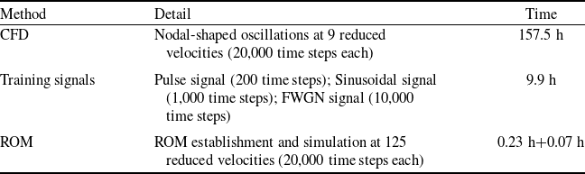
Figure 12 gives the comparison of the buffeting oscillations between the ROM-based simulation and the CFD-based simulation at different reduced velocities. Moreover, Fig. 13 gives the dominant frequencies of the dynamic responses at the same range of reduced velocities. In Fig. 13, the 1st frequency and the 2nd frequency correspond to the highest peak and the second-highest peak, respectively. The 1st and 2nd frequencies of the plunge exchange positions, showing that the major frequency components of aerodynamic forces are different at different frequencies. The comparison shows that the nonlinear ROM has an excellent ability to predict the nodal-shaped oscillations at different reduced velocities. Then, Table 2 gives the comparison of the total CPU times for the CFD simulation and the nonlinear ROM simulation for the aeroelastic phenomena at different reduced velocities. The results well indicate that the nonlinear ROM has an efficient ability to model the aeroelastic phenomena with high accuracy, even when the time of generating the training signals is taken into account.

Table 2.

Comparison of the CPU times for CFD and nonlinear ROM simulations

Figure 12.

Amplitudes of nodal-shaped oscillations vs. dimensionless velocity.

Figure 13.

Frequencies of nodal-shaped oscillations vs. dimensionless velocity.

4.3. Predictions of open-loop buffeting behaviours

This subsection compares the ASE behaviours induced via the control surface motions at two reduced velocities, with input signals of different amplitudes and frequencies. At the low reduced velocities, the amplitudes of the structural vibrations are small and the ASE system presents linear characteristics. When the reduced velocities go up, the ASE system presents nonlinear characteristics for large amplitudes of the structural vibrations.

The ASE behaviours at $V_\infty ^ * = 0.320$ with sinusoidal input are presented in Fig. 14. The amplitude and the frequency of the sinusoidal input are chosen as 1 deg and 3.6 Hz, which is close to the uncoupled natural frequencies of the plunge. The transient response of the ASE systems can be accurately reproduced via the nonlinear ROM. As time goes on, the transient response disappears and the sinusoidal steady-state response appears because of the linear behaviour of the ASE system at low reduced velocity. Because of the fidelity importance of the frequency response of a linear system to be controlled, the comparison is made in Fig. 15 for the frequency responses via CFD-based and ROM-based ASE systems. The figure shows that the frequency responses are the same when the input signal amplitudes are 1 deg and 3 deg, respectively. This evidence verifies again that the ASE system at $V_\infty ^ * = 0.320$ presents linear characteristics. Hence, the CFD-based ASE systems can be replaced with the ROM-based in the design of the active control system at low reduced velocities.

Figure 14.

Dynamic response of the aeroservoelastic model with the sinusoidal input at $V_\infty ^ * = 0.320$ .

Figure 15.

Frequency-response function at $V_\infty ^ * = 0.320$ .

The ASE behaviours at $V_\infty ^ * = 0.555$ under the sinusoidal input of different amplitudes and frequencies are also compared in the time domain. The responses under the sinusoidal input with 1deg and 3.6 Hz are shown in Fig. 16. The response is superimposed via two frequencies – one is the frequency of the control surface motions and the other is the frequency of the aerodynamic forces. The responses under the sinusoidal input with 3 deg and different frequencies are presented in Figs 17 and 18. On one hand, the aerodynamic forces are stimulated with nonlinear characteristics with larger amplitudes of input signals and structural vibrations. On the other hand, the rise and fall of the amplitudes of the structural vibrations in both figures are caused by the large nonlinear characteristics of the aerodynamic forces. The ROM-based ASE responses are compared with the CFD-based ones in Figs 17 and 18. The comparison shows that the ROM-based ASE models can accurately simulate the nonlinear characteristics of the aerodynamic forces for a long duration.

Figure 16.

Dynamic response stimulated via the sinusoidal input with 1 deg and 3.6 Hz at $V_\infty ^ * = 0.555$ .

Figure 17.

Dynamic response stimulated via the sinusoidal input with 3 deg and 3.6 Hz at $V_\infty ^ * = 0.555$ .

Figure 18.

Dynamic response stimulated via the sinusoidal input with 3 deg and 3.8 Hz at $V_\infty ^ * = 0.555$ .

4.4 Performance for transonic buffeting control

This subsection gives the detailed parameters of the controller and verifies its control performance for the transonic buffeting vibrations of the ASE system. The order of the linear ACRC controller is set to 2. Based on the adjustment principles, the parameters are eventually determined as ${\bar b_0}$ = $-$ 40000, ${\omega _o}$ =250 and ${\omega _c}$ =18.

To check the control performance of the controller in the transonic region, the closed-loop ASE analysis is implemented at $V_\infty ^ * = 0.56$ and $V_\infty ^ * = 0.621$ . The acceleration signal and the control command are given in Figs 19 and 20 to show the effectiveness of the controller at $V_\infty ^ * = 0.56$ and $V_\infty ^ * = 0.621$ , respectively. The controller is first switched off and then switched on after a short moment. As shown in Fig. 19, the flutter instabilities can be observed before the controller is switched on. However, the flutter instabilities disappear when the controller is switched on at the moment of 25 s. A similar phenomenon can also occur for the open/closed ASE modeling at $V_\infty ^ * = 0.621$ . The structural vibration for the first 5 s in Fig. 20 is actually the nodal-shaped oscillations in Fig. 8. When the controller is switched on at the moment of 5 s, the unstable structural vibrations, i.e. the nodal-shaped oscillations, gradually become stable as time goes on. The amplitudes of the control command are lower than 6deg in Fig. 19 and lower than 4.5 deg in Fig. 20. However, the on/off control simulations only verify the control performance of the controller. The controller is actually switched on during the whole process, and thus the control command will be much lower than that in the simulations. The controller increases the unstable boundary by 21.5%, from $V_\infty ^ * = 0.557$ to $V_\infty ^ * = 0.677$ based on the ROM-based ASE systems. Figure 21 shows the root-of-mean-squared (RMS) value of the acceleration response and the control surface at different reduced velocities under the same initial conditions. As shown in the figure, the RMS values of deflection of the control surface increase with an increase in the reduced velocities and the increasing rate becomes much larger when the reduced velocity is close to the unstable boundary of the closed-loop ASE system.

Figure 19.

Input and output signals of the controller for $V_\infty ^ * = 0.56$ .

Figure 20.

Input and output signals of the controller for $V_\infty ^ * = 0.621$ .

Figure 21.

RMS responses for the closed-loop system.

Now, the anti-interference abilities are checked for the present controller via numerical simulations, where the acceleration signal is mixed with the FWGN signal to simulate the effects of measured noises. The simulations are carried out at two typical reduced velocities $V_\infty ^ * = 0.56$ and $V_\infty ^ * = 0.621$ . The amplitude of the noise is 10% of the maximal value of the accelerations in each simulation, and the frequency ranges of the noises are both from 20 to 50 Hz. The time histories of the acceleration signals and control commands in two typical reduced velocities are given in Figs 22 and 23, respectively. The changing process of the controller is the same as the process in the simulations without FWGN. In the two figures, the structural vibrations cannot be suppressed completely due to the noise interference, but they can be reduced to a small range. That is, the controller has good anti-interference abilities to suppress the structural instability with measured noises. The effects of measured noises at other reduced velocities are also verified. The RMS responses of the real acceleration and the control surface at different reduced velocities under zero initial conditions and the same measured noise are shown in Fig. 24. Although the RMS deflection of the real acceleration increases with an increase in the reduced velocity, the RMS deflection of the control surface nearly remains constant. The results make it clear that the energy consumed by the controller for suppressing the measured noise is the same for different velocities. However, the amplitude of structural vibration induced via the measured noise can be larger for higher reduced velocity.

Figure 22.

Input and output signals of the controller with high-frequency noise for $V_\infty ^ * = 0.56$ .

Figure 23.

Input and output signals of the controller with high-frequency noise for $V_\infty ^ * = 0.621$ .

Figure 23 Long description

The image contains two line graphs. Panel A: The top graph is a line graph showing the acceleration signal over time. The x-axis represents time in seconds, ranging from 0 to 10 seconds. The y-axis represents the acceleration signal in feet per second squared, ranging from -200 to 200. The graph includes two lines: a red dotted line representing the true output and a black solid line representing the measured output. The data shows oscillatory behavior with decreasing amplitude over time. Panel B: The bottom graph is a line graph showing the control command over time. The x-axis represents time in seconds, ranging from 0 to 10 seconds. The y-axis represents the control command in degrees, ranging from -6 to 6. The graph shows a line that starts at 0, remains flat until around 4 seconds, and then exhibits oscillatory behavior with decreasing amplitude over time.

Figure 24.

RMS responses for the closed-loop system with measured noise.

Finally, the verification turns to the ability of the controller for a possible time delay in the control loop. The following simulations present the performance of the controller with a time delay for two reduced velocities. The results show that the tolerance interval of the time delay at $V_\infty ^ * = 0.56$ is 0∼50 ms, while the tolerance interval of the time delay at $V_\infty ^ * = 0.621$ decreases to 0∼5 ms. Figures 25 and 26 give the numerical simulations for $V_\infty ^ * = 0.56$ with a time delay of 50 ms and for $V_\infty ^ * = 0.621$ with a time delay of 5 ms, respectively. The acceleration signals in two simulations decrease slowly, and the controller fails for larger time delays. Unlike the controller’s anti-interference capabilities, introducing a time delay in the control loop negatively affects the controller’s ability to suppress structural instabilities when there are nonlinearities introduced by buffet. However, the controller can accept a short time delay to suppress the transonic buffeting vibrations.

Figure 25.

Input and output signals of the controller with a time delay for $V_\infty ^ * = 0.56$ .

Figure 26.

Input and output signals of the controller with a time delay for $V_\infty ^ * = 0.621$ .