





1. Introduction
Particle-laden flows are ubiquitous in nature and engineering (Brandt & Coletti Reference Brandt and Coletti2022; Marchioli et al. Reference Marchioli2025, Reference Marchioli, Rosti and Verhille2026). Examples include cloud droplets and volcanic ashes in planetary atmospheres (Rose & Durant Reference Rose and Durant2009; Mellado Reference Mellado2017), the formation of protoplanetary disks (Birnstiel Reference Birnstiel2024), the dispersal of phytoplankton and microplastics in the ocean (Borgnino et al. Reference Borgnino, Arrieta, Boffetta, De Lillo and Tuval2019; Sugathapala et al. Reference Sugathapala, Capuano, Brandt, Iudicone and Sardina2025), the transport of blood cells (Freund Reference Freund2014) and industrial processes such as flue gas scrubbing (Lee et al. Reference Lee, Mohan, Byeon, Lim and Hong2013) and fuel atomisation in spray combustion (Jenny et al. Reference Jenny, Roekaerts and Beishuizen2012). These phenomena see a turbulent carrier flow transporting and interacting with a solid (or liquid) suspension that can either energise or weaken its motion. The nature of this modulation depends on factors such as the relative size of the particle and the turbulent eddies (Gore & Crowe Reference Gore and Crowe1989), as well as the inertia and degree of dilution of the suspension (Balachandar & Eaton Reference Balachandar and Eaton2010). A suspension is considered dilute or dense in the limit of low or high volume fraction
 $\varPhi _p = \mathcal{V}_p/(\mathcal{V}_f + \mathcal{V}_p)$
, where
 $\mathcal{V}_f$
and
 $\mathcal{V}_p$
denote the volumes occupied by the fluid and dispersed phases, respectively. The threshold also depends on the density ratio
 $\varPsi _p = \rho _p/\rho _{\kern-1pt f}$
, where
 $\rho _p$
and
 $\rho _{\kern-1pt f}$
are the particle and fluid densities, respectively, and on the particle size
 $D$
(Elghobashi Reference Elghobashi1994; Balachandar & Eaton Reference Balachandar and Eaton2010). In general, when
 $D$
is much smaller than the Kolmogorov length scale
 $\eta$
, the motion of the particles is primarily governed by that of the local fluid, the strength of their response being modulated by inertia. Particles of negligible inertia behave as pure tracers and follow the motion of the carrier flow, while particles of large inertia are only weakly affected by the surface stresses induced by the carrier flow and do not follow its streamlines. Particles of moderate inertia are expected to be only partially influenced by the carrier flow, their trajectory departing from its streamlines in the presence of intense velocity gradients. This centrifugal mechanism was proposed by Maxey (Reference Maxey1987), who showed that small, light spheres segregate in regions of low vorticity and high strain, and that this behaviour intensifies for increasing particle mass. His predictions were later confirmed numerically by Squires & Eaton (Reference Squires and Eaton1990). This preferential sampling of the flow has been indicated as a key process in the formation and evolution of clusters in homogeneous and isotropic turbulence (see the reviews of Balachandar & Eaton Reference Balachandar and Eaton2010 and Brandt & Coletti Reference Brandt and Coletti2022). The sweep-stick mechanism of Goto & Vassilicos (Reference Goto and Vassilicos2008) has also been proposed to account for preferential sampling in flows laden with smaller-than-Kolmogorov and finite-size particles (Yoshimoto & Goto Reference Yoshimoto and Goto2007; Uhlmann & Chouippe Reference Uhlmann and Chouippe2017).
When forming dilute suspensions, low-inertia, smaller-than-Kolmogorov particles behave essentially as passive tracers of a one-way coupled mechanical system (Volk et al. Reference Volk, Calzavarini, Verhille, Lohse, Mordant, Pinton and Toschi2008; Sumbekova et al. Reference Sumbekova, Cartellier, Aliseda and Bourgoin2017). These flows have been extensively investigated with the aid of point-particle direct numerical simulations (DNSs) where the motion of each particle is governed by a Lagrangian tracker (Maxey & Riley Reference Maxey and Riley1983; Matsuda et al. Reference Matsuda, Yoshimatsu and Schneider2024). Point-particle DNSs rely on the assumption of uniform flow properties across larger-than-particle distances
 $D/\eta \ll 1$
, meaning that the sub-Kolmogorov scales need not be resolved (Brandt & Coletti Reference Brandt and Coletti2022). Although enormous efforts have been made in the development of two-way coupling models (Balachandar et al. Reference Balachandar, Liu and Lakhote2019), point-particle DNSs are yet to provide an accurate and complete description of the particle–fluid interaction when
 $D/\eta =O(1)$
, a condition typical of several practical scenarios in which the dispersed phase modulates the turbulence (Tanaka & Eaton Reference Tanaka and Eaton2010; Luo et al. Reference Luo, Wang, Li, Tan and Fan2017; Oka & Goto Reference Oka and Goto2022). In recent years, particle-resolved direct numerical simulations (PR-DNSs) based on the immersed boundary method (IBM) have cast new light on the interphase coupling in suspensions of larger-than-Kolmogorov (
 $D/\eta \gg 1$
) spherical particles (Kajishima et al. Reference Kajishima, Takiguchi, Hamasaki and Miyake2001; Uhlmann Reference Uhlmann2005; Breugem Reference Breugem2012; Kempe & Fröhlich Reference Kempe and Fröhlich2012; Hori et al. Reference Hori, Rosti and Takagi2022). To name a few, we recall the works by Lucci et al. (Reference Lucci, Ferrante and Elghobashi2010), Uhlmann & Chouippe (Reference Uhlmann and Chouippe2017), Chouippe & Uhlmann (Reference Chouippe and Uhlmann2019), Oka & Goto (Reference Oka and Goto2022), Olivieri et al. (Reference Olivieri, Cannon and Rosti2022), Chiarini & Rosti (Reference Chiarini and Rosti2024) and Cannon et al. (Reference Cannon, Olivieri and Rosti2024) for homogeneous isotropic turbulence, and those by Uhlmann (Reference Uhlmann2008), Ardekani & Brandt (Reference Ardekani and Brandt2019), Rosti & Brandt (Reference Rosti and Brandt2020), Costa et al. (Reference Costa, Brandt and Picano2021) and Gao et al. (Reference Gao, Samtaney and Richter2023) for turbulent channel flows. These works highlight the importance of the ratio
 $D/\eta$
on turbulence modulation: inertial-scale particles provide a spectral shortcut by extracting energy from the large scales and reinjecting it into the small ones (Lucci et al. Reference Lucci, Ferrante and Elghobashi2010; Oka & Goto Reference Oka and Goto2022; Chiarini & Rosti Reference Chiarini and Rosti2024), whereas Kolmogorov-size particles absorb the carrier flow’s kinetic energy (Tanaka & Eaton Reference Tanaka and Eaton2010) and may impose a decay rate of the energy spectrum proportional to the inverse fourth power of their spatial wavenumber (Wang et al. Reference Wang, Ayala, Gao, Andersen and Mathews2014; Chiarini et al. Reference Chiarini, Tandurella and Rosti2025). The exact conditions under which turbulence enhancement or attenuation occur remain unclear (Marchioli et al. Reference Marchioli2025) and likely result from a non-trivial interplay between several parameters (Tanaka & Eaton Reference Tanaka and Eaton2008). In the absence of gravity, the PR-DNSs of Lucci et al. (Reference Lucci, Ferrante and Elghobashi2010) reported turbulence attenuation in triperiodic homogeneous isotropic turbulence laden with suspensions of Taylor-scale spheres with
 $0.01 \leq \varPhi _p \leq 0.1$
and
 $2.56 \leq \varPsi _p \leq 10$
, whereas Chiarini & Rosti (Reference Chiarini and Rosti2024) observed a non-monotonic dependence of the kinetic energy on the mass fraction
 $M_p=\varPsi_p\varPhi_p(\varPsi_p\varPhi_p+1-\varPhi_p)^{-1}$
and the size ratio
 $D/\eta$
for
 $M_p \geq 0.45$
and
 $D/\eta \leq 64$
. In the latter regime, the enhancement of turbulent kinetic energy was associated with a large-scale anisotropic modulation (Chiarini et al. Reference Chiarini, Cannon and Rosti2024). Turbulence enhancement has also been observed experimentally in settling suspensions of heavy sub-Kolmogorov particles with higher density ratios
 $\varPsi _p = O(10^3)$
(Yang & Shy Reference Yang and Shy2005) and has been attributed to the release of gravitational potential energy (Hassaini & Coletti Reference Hassaini and Coletti2022).
Small, heavy particles can attenuate the turbulent fluctuations just like large, light ones (Oka & Goto Reference Oka and Goto2022). Along with the volume fraction
 $\varPhi _p$
and the size ratio
 $D/\eta$
, the particle-to-fluid density ratio
 $\varPsi _p$
plays a key role on the interphase coupling (Brandt & Coletti Reference Brandt and Coletti2022). Yu et al. (Reference Yu, Lin, Shao and Wang2017) performed PR-DNSs with a direct forcing-fictitious domain method to study the effect of increasing
 $\varPsi _p$
in the range
 $1{-}100$
on a turbulent channel flow at a friction Reynolds number
 $ \textit{Re}_\tau =180$
and volume fraction
 $\varPhi _p=8.4\times 10^{-3}$
. They considered two sets of spherical particles of diameter
 $0.1$
and
 $0.2$
times the channel half-width, which correspond to
 $D/\eta \cong 5$
and
 $D/\eta \cong 10$
, respectively. They reported a non-monotonic trend of the total drag, which first increased along with the viscous dissipation for
 $\varPsi _p\leq 10$
, but diminished as the formation of near-wall streamwise vortices was inhibited (Lucci et al. Reference Lucci, Ferrante and Elghobashi2010). Tavanashad et al. (Reference Tavanashad, Passalacqua, Fox and Subramaniam2019) investigated non-dilute populations of larger-than-Kolmogorov spherical particles by performing PR-DNSs on a triperiodic box. They considered several orders of magnitude of
 $\varPsi _p$
(
 $10^{-3}{-}10^{3}$
) and showed that heavier suspensions extract more kinetic energy from the carrier flow. Although they did not report the Kolmogorov length scale nor the Reynolds number, they used two sets of particles with diameter
 $20$
and
 $30$
times larger than the grid cell. More recently, Shen et al. (Reference Shen, Peng, Lu and Wang2024) performed PR-DNSs using a lattice-Boltzmann method to study the effect of variable particle density on finite-size spherical particles on a turbulent channel flow, with particles in the range
 $6\lesssim D/\eta \lesssim 23$
. Two-way coupled point-particle DNSs have also been employed to study the effect of particle inertia in suspensions of smaller-than-Kolmogorov spherical particles. Mortimer & Fairweather (Reference Mortimer and Fairweather2020) studied the effect of increasing
 $\varPsi _p$
on near-wall coherent structures in a channel flow laden with
 $300\,000$
spheres at a friction Reynolds number
 $ \textit{Re}_\tau =180$
and volume fraction
 $\varPhi _p=10^{-4}$
. Their results showed a monotonic attenuation of the turbulent fluctuations in the near-wall region with increasing particle density. Gualtieri et al. (Reference Gualtieri, Battista, Salvadore and Casciola2023) conducted an extensive simulation campaign of non-dilute suspensions (
 $\varPhi _p=0.4$
) of smaller-than-Kolmogorov spheres in channel flows and concluded that dense particles deplete a considerable amount of turbulent kinetic energy. Consistently with the results of Yu et al. (Reference Yu, Lin, Shao and Wang2017), they reported an increase in friction drag in the presence of light particles, which acted as a source of turbulent kinetic energy near the wall.
Although predominantly studied numerically, particle-laden turbulent flows have also been the subject of several experimental studies. Most laboratory measurements have focused on suspensions of particles smaller than the Kolmogorov scale (
 $D/\eta \ll 1$
, e.g. Yang & Shy Reference Yang and Shy2005; Salazar et al. Reference Salazar, De Jong, Cao, Woodward, Meng and Collins2008; Saw et al. Reference Saw, Shaw, Ayyalasomayajula, Chuang and Gylfason2008; Good et al. Reference Good, Ireland, Bewley, Bodenschatz, Collins and Warhaft2014; Obligado et al. Reference Obligado, Teitelbaum, Cartellier, Mininni and Bourgoin2014; Sumbekova et al. Reference Sumbekova, Cartellier, Aliseda and Bourgoin2017; Hassaini & Coletti Reference Hassaini and Coletti2022; Ferran et al. Reference Ferran, Machicoane, Aliseda and Obligado2023; Hassaini et al. Reference Hassaini, Petersen and Coletti2023), whereas fewer works have addressed suspensions of particles larger than the Kolmogorov scale (
 $D/\eta \gg 1$
). Tsuji & Morikawa (Reference Tsuji and Morikawa1982) investigated the influence of particle size on turbulence modulation in gas–solid suspensions. They considered a horizontal pipe of diameter
 $30\,\textrm {mm}$
with mean velocity between
 $6$
and
 $20\,\textrm {m s}^{-1}$
, and reported turbulence attenuation and enhancement in the presence of relatively small (
 $D=0.2\,\text{mm}$
) and large (
 $D=3.4\,\text{mm}$
) particles, respectively. Brown et al. (Reference Brown, Warhaft and Voth2009) studied von Kármán turbulence generated between counter-rotating disks at Taylor–Reynolds numbers
 $400\lt Re_\lambda \lt 815$
. The flow was laden with neutrally buoyant polystyrene spheres whose size spanned from the dissipative range to the inertial subrange (
 $0.4\lt D/\eta \lt 27$
). They reported that the acceleration variance of the largest particles (
 $D/\eta \gt 5$
) follows the scaling
 $D^{-2/3}$
proposed by Voth et al. (Reference Voth, La Porta, Crawford, Alexander and Bodenschatz2002). Fiabane et al. (Reference Fiabane, Zimmermann, Volk, Pinton and Bourgoin2012) investigated homogeneous isotropic turbulence laden with particles of size
 $4.5\lt D/\eta \lt 17$
in an icosahedral vessel. Using Voronoi tessellation analysis, they showed that neutrally buoyant particles do not cluster, whereas heavy particles cluster independently of their size. More recently, Hoque et al. (Reference Hoque, Mitra, Sathe, Joshi and Evans2016) examined the effect of isolated glass particles in the range
 $10\lt D/\eta \lt 77$
in turbulence generated by an oscillating grid. They found that turbulence modulation depends critically on the ratio between the particle diameter and the integral length scale (Gore & Crowe Reference Gore and Crowe1989). Among the experiments on Kolmogorov-size particles, we recall Hwang & Eaton (Reference Hwang and Eaton2006b
), who investigated the sedimentation of glass spheres with
 $\varPsi _p \cong 2500$
, Poelma et al. (Reference Poelma, Westerweel and Ooms2007), who examined the effect of heavy particles on the decay of grid-generated turbulence and Tanaka & Eaton (Reference Tanaka and Eaton2010), who performed high-resolution particle image velocimetry. They concluded that particles with a smaller diameter and a higher density induce the strongest attenuation in steady-state homogeneous and isotropic turbulence. Laboratory experiments and point-particle DNS of turbulent flows laden with Kolmogorov-scale solid particles and bubbles at
 $ \textit{Re}_\lambda \leq 180$
were compared by Volk et al. (Reference Volk, Calzavarini, Verhille, Lohse, Mordant, Pinton and Toschi2008) and Tagawa et al. (Reference Tagawa, Martìnez Mercado, Prakash, Calzavarini, Sun and Lohse2012). The latter, who employed the datasets of Martínez Mercado et al. (Reference Martínez Mercado, Prakash, Tagawa, Sun and Lohse2012), reported stronger clustering at higher
 $ \textit{Re}_\lambda$
.
Gravity induces settling or rising of the dispersed phase in non-neutrally buoyant suspensions, leading to a departure from isotropy and altering both the collective dynamics of the particles and the statistics of the carrier flow substantially (Brandt & Coletti Reference Brandt and Coletti2022). Because laboratory studies in microgravity remain extremely challenging (Fallon & Rogers Reference Fallon and Rogers2002; Hwang & Eaton Reference Hwang and Eaton2006b
), terrestrial measurements are compared with numerical simulations of homogeneous isotropic turbulence that neglect gravity (Tagawa et al. Reference Tagawa, Martìnez Mercado, Prakash, Calzavarini, Sun and Lohse2012). Particle-resolved numerical simulations provide a means to investigate isotropic flows in the absence of gravity, but are limited by the high spatial resolution required to accurately resolve the fluid field at sub-particle scales. Resolving the sub-particle motion via PR-DNSs requires grid spacings well below
 $\eta$
, thus rendering the computational cost prohibitive even at moderate Reynolds numbers. For this reason, a broad body of numerical work has focused on the limits
 $D\ll \eta$
and
 $D\gg 1$
, while Kolmogorov-size spheres have received far less attention. Using the IBM proposed by Uhlmann (Reference Uhlmann2005), Uhlmann & Chouippe (Reference Uhlmann and Chouippe2017) were able to investigate a particle laden triperiodic flow at
 $ \textit{Re}_\lambda \cong 115$
and with
 $D/\eta =5$
, slightly above the Kolmogorov scale. Schneiders et al. (Reference Schneiders, Meinke and Schröder2017) conducted PR-DNSs of a triperiodic turbulent flow laden Kolmogorov-size spheres with
 $D/\eta \cong 1.32$
using a Cartesian cut-cell method. They considered a suspension of
 $45\,000$
particles in a decaying homogeneous and isotropic turbulent flow and density ratios
 $\varPsi _p$
in the range
 $40{-}5000$
. The enormous computational burden entailed by the resolution of sub-Kolmogorov motions limited the initial value of the Taylor-based Reynolds number to
 $70$
. Chiarini et al. (Reference Chiarini, Tandurella and Rosti2025) used the IBM of Hori et al. (Reference Hori, Rosti and Takagi2022) to characterise the behaviour of a suspension of particles with diameter
 $D\cong \eta$
and
 $\varPsi _p=5$
,
 $100$
. They compared their results with those obtained from point-particle simulations and reported significant discrepancies for the cases with the highest density ratio.
1.1. Objectives and outline
Particle-resolved DNS of Kolmogorov-scale spheres in homogeneous isotropic turbulence have either considered decaying carrier flows without a fully developed inertial subrange at small
 $ \textit{Re}_\lambda$
(Schneiders et al. Reference Schneiders, Meinke and Schröder2017), or have been restricted to relatively low density ratios
 $\varPsi _p \leq 100$
(Uhlmann & Chouippe Reference Uhlmann and Chouippe2017; Chiarini et al. Reference Chiarini, Tandurella and Rosti2025). However, many natural and industrial flows exhibit a fully developed inertial subrange and involve dense suspensions of high-inertia particles
 $\varPsi _p=O(10^3)$
that can fundamentally alter the carrier-flow dynamics (Rose & Durant Reference Rose and Durant2009; Jenny et al. Reference Jenny, Roekaerts and Beishuizen2012).
The primary objective of this work is to quantify the impact of suspensions of heavy Kolmogorov-size spheres on the turbulent cascade, the scale-by-scale energy transfer and the small-scale intermittency of the carrier flow, as well as to assess how increasing particle inertia shapes the collective dynamics of the dispersed phase and the structure of particle clusters. To this end, we perform large-scale PR-DNSs of a homogeneous, isotropic, triply periodic turbulent flow. A Taylor-scale Reynolds number of
 $ \textit{Re}_\lambda \cong 150$
is selected to ensure adequate scale separation within the inertial subrange in the unladen case. We consider a fixed particle volume fraction
 $\varPhi _p=10^{-3}$
and density ratios up to
 $\varPsi _p=1500$
, a regime that lies beyond the range of validity of point-particle approaches and is directly relevant to natural and industrial flows (Brandt & Coletti Reference Brandt and Coletti2022; Marchioli et al. Reference Marchioli2025).
The paper is organised as follows. The numerical method and its implementation are described in § 2, and the post-processing procedures and results are presented in § 3. In particular, the bulk statistics of the carrier flow are discussed in § 3.1, followed by energy spectra and structure functions in § 3.2, the scale-by-scale energy budget in § 3.3 and the analysis of the velocity-gradient tensor in § 3.4. Particle dynamics and clustering statistics are examined in §§ 3.5 and 3.6, respectively, while the particles’ preferential sampling is discussed in § 3.7. Finally, conclusions are drawn in § 4.
2. Direct numerical simulations
2.1. Mathematical formulation
We consider a triply periodic cubic domain of volume
 $\mathcal{V}_L=L^3$
, where
 $L$
is the side length of the cube. The carrier flow (fluid phase) is governed by the incompressible Navier–Stokes equations for momentum balance and the continuity constraint
 \begin{align} \frac {\partial u_i}{\partial t} + \frac {\partial u_{\kern-1pt j} u_i}{\partial x_{\kern-1pt j}} = \frac {1}{\rho _{\kern-1pt f}}\frac {\partial \sigma _{\textit{ij}}}{\partial x_{\kern-1pt j}} + f_i^{\textit{ABC}} + f_i^{\textit{part}}, \\[-28pt] \nonumber \end{align}
 \begin{align} \frac {\partial u_k}{\partial x_k} = 0, \\[0pt] \nonumber \end{align}
where Einstein summation over repeated indices is implied. Here,
 $u_i$
is the fluid velocity,
 $\rho _{\kern-1pt f}$
the fluid density and
 $f_i^{\textit{part}}$
is the IBM forcing exerted by the solid particles on the fluid (Hori et al. Reference Hori, Rosti and Takagi2022). The large-scale volume forcing
 $f_i^{\textit{ABC}}$
is of the Arnold–Beltrami–Childress (ABC) type (Arnold Reference Arnold1965, p. 20)
 \begin{align} f_x^{\textit{ABC}} &= F_0 \left [ \cos \left (\frac {2\pi }{L}y\right ) + \sin \left (\frac {2\pi }{L}z\right ) \right ] \!, \\[-12pt] \nonumber \end{align}
 \begin{align} f_y^{\textit{ABC}} &= F_0 \left [ \cos \left (\frac {2\pi }{L}z\right ) + \sin \left (\frac {2\pi }{L}x\right ) \right ]\!, \\[-12pt] \nonumber \end{align}
 \begin{align} f_z^{\textit{ABC}} &= F_0 \left [ \cos \left (\frac {2\pi }{L}x\right ) + \sin \left (\frac {2\pi }{L}y\right ) \right ]\!, \\[10pt] \nonumber \end{align}
and has an amplitude
 $F_0$
with units of force per mass. Because the carrier flow is Newtonian and incompressible, the stress tensor
 $\sigma _{\textit{ij}}$
reads
 \begin{align} \sigma _{\textit{ij}} = - p \delta _{\textit{ij}} + 2\mu_{\kern-1pt f} S_{\textit{ij}}, \end{align}
where
 $p$
is the fluid pressure,
 $\delta _{\textit{ij}}$
is the Kronecker delta,
 $\mu_{\kern-1pt f}$
is the dynamic viscosity and
 $S_{\textit{ij}} = (\partial _{\kern-1pt j}u_i + \partial _iu_{\kern-1pt j})/2$
is the symmetric part of the velocity-gradient tensor
 $\partial _{\kern-1pt j}u_i$
. From this point onwards, the kinematic viscosity of the fluid phase
 $\nu_{\kern-1pt f}=\mu_{\kern-1pt f}/\rho _{\kern-1pt f}$
will be used.
The velocity of a point inside a solid spherical particle is due to the contribution of the translational velocity and the rotation around the particle centre
 $U_i = \tilde U_{i} + \epsilon _{\textit{ijk}} \varOmega _{j} R_k$
, where
 $\varOmega_{\kern-1pt j}$
is the particle rotational velocity,
 $\epsilon _{\textit{ijk}}$
the Levi-Civita tensor and
 $R_k$
the radial distance from the particle centre. The time evolution of the translational velocity
 $\tilde {U}_i$
and the angular velocity
 $\varOmega_{\kern-1pt j}$
is governed by the Newton–Euler equations
 \begin{align} m_p \frac {\mathrm{d} \tilde U_i}{\mathrm{d} t} &= \oint _{\partial \mathcal{V}_p} \sigma _{\textit{ij}} n_j \mathrm{d}\left (\partial \mathcal{V}\right ) + F_{i}^{\textit{col}}, \\[-12pt] \nonumber \end{align}
 \begin{align} \mathcal{I}_p \frac {\mathrm{d} \varOmega _i}{\mathrm{d} t} &= \oint _{\partial \mathcal{V}_p} \epsilon _{\textit{ijk}} R_j \sigma _{kl} n_l \mathrm{d}\left (\partial \mathcal{V}\right ). \\[10pt] \nonumber \end{align}
Here,
 $F^{\textit{col}}$
is the force exerted by inter-particle collisions,
 $\sigma _{\textit{ij}}$
is defined in (2.3),
 $n_i$
is the outer normal to the particle surface,
 $m_p = (\pi /6) \rho _p D^3$
and
 $\mathcal{I}_p = (m_p/10) D^2$
are the particle mass and moment of inertia, respectively, and
 $D$
is the particle diameter. No-slip and no-penetration conditions are applied at the particle surface
 $u_i = U_i$
, where the velocity of the fluid and solid phase match. The particle translational velocity is integrated at every time step to update the particle location
 $X_i$
, where
 $\tilde U_i = \mathrm{d} X_i/\mathrm{d} t$
. Inter-particle collisions are handled with the mass–spring–dash pot model of Tsuji et al. (Reference Tsuji, Kawaguchi and Tanaka1993) and Costa et al. (Reference Costa, Boersma, Westerweel and Breugem2015). A repulsive force acts on the particles as soon as their volumes overlap, i.e. when the distance between their centres falls below
 $D$
.
The parameters common to all simulations are summarised in table 1. The Reynolds number based on the side length of the domain and the characteristic velocity
 $(F_0L)^{1/2}$
is
 $ \textit{Re}_L\equiv F_0^{1/2}L^{3/2}/\nu_{\kern-1pt f} = 1761$
. We consider a monodisperse (i.e. uniform in size) population of
 $N=74\,208$
spherical particles with diameter
 $D \cong 0.003L$
that matches the Kolmogorov scale
 $\eta$
in all the cases examined. The particle diameter is kept constant and chosen to match the space–time average of the Kolmogorov scale in the unladen case (
 $M_p=0$
). As verified a posteriori, moderate variations in the dissipation rate with the mass fraction
 $M_p$
lead to negligible changes in
 $\eta$
(see discussion in § 3.1). The volume fraction of the solid phase is kept constant
 $\varPhi _p = (\pi N/6) (D/L)^3 = 10^{-3}$
across all simulations. Thus, the mass fraction is determined solely by the density ratio
 $\varPsi _p= \rho _p/\rho _{\kern-1pt f}$
through the relation
 \begin{align} M_p = \frac {\varPsi _p\varPhi _p}{1 - \varPhi _p + \varPsi _p\varPhi _p}. \end{align}
Four laden cases with density ratio
 $\varPsi _p = 100$
,
 $250$
,
 $666$
,
 $1499$
and mass fraction
 $M_p=0.1$
,
 $0.2$
,
 $0.4$
,
 $0.6$
are compared with the unladen case (
 $\varPhi _p=M_p=0$
). These values of
 $M_p$
match those used in the experiments of Tanaka & Eaton (Reference Tanaka and Eaton2010) (see table 3 therein).
Parameters common to all simulations:
 $N$
is the total number of particles,
 $n_{\textit{grid}}$
the number of grid points in the uniform Cartesian mesh,
 $\varPhi _p$
the particle volume fraction,
 $D$
the particle diameter and
 $ \textit{Re}_L\equiv (F_0L^3)^{1/2}/\nu_{\kern-1pt f}$
the Reynolds number defined on the characteristic velocity
 $(F_0L)^{1/2}$
. Here,
 $F_0=5$
is the amplitude of the ABC volume forcing (2.2) and has units of force per mass,
 $L=2\pi$
is the side length of the cubic domain and
 $\nu_{\kern-1pt f}=\mu_{\kern-1pt f}/\rho _{\kern-1pt f}=1/50.$
.

Table 1. Long description
A table summarizing parameters common to all simulations. The table has one row and five columns. Column headers are N, n_grid, Φ_p, D/L, and Re_L. Row 1: N, 74208; n_grid, 2048^3; Φ_p, 10^−3; D/L, 0.003; Re_L, 1761.
2.2. Numerical method
The numerical method described in this section is implemented on the in-house Fortran code Fujin (Rosti Reference Rosti2026). The momentum equation for the fluid phase (2.1a
) is advanced in time with a fractional step method (Amsden & Harlow Reference Amsden and Harlow1970; Kim et al. Reference Kim, Moin and Moser1987; Tomé et al. Reference Tomé, Duffy and McKee1996). The nonlinear and viscous terms in (2.1a
) are discretised using an Adams–Bashforth scheme in the predictor step, while incompressibility is enforced by solving the Poisson equation for the pressure with a fast Fourier transform. The interplay of the fluid phase and the solid spheres is taken into account with the Eulerian IBM described by Hori et al. (Reference Hori, Rosti and Takagi2022). A fixed-radius, near-neighbours search algorithm is used to reduce the computational cost of the collisions from
 $O(N^2)$
to
 $O(N)$
(Monti et al. Reference Monti, Rathee, Shen and Rosti2021). The code uses a two-dimensional Cartesian parallelisation provided by the message-passage interface library. The triperiodic cubic domain is discretised using an uniform Cartesian grid of
 $n_{\textit{grid}} = 2048^3$
points. The computations were performed using 4096 cores on the CPU-based cluster Deigo at the Okinawa Institute for Science and Technology.
The laden case with mass fraction
 $M_p=0.1$
was initialised by seeding a fully developed turbulent flow with
 $N$
spherical particles. The procedure is the following. The coordinates
 $X_i$
of each particle are sampled sequentially from a uniform distribution using a random-number generator in Matlab. If a generated particle does not overlap with any previously placed particle, it is accepted; otherwise, it is rejected and the procedure is repeated until all initial positions are assigned. The particles are initially at rest (
 $\tilde U_i= \varOmega _i=0$
) and subsequently accelerate under the hydrodynamic forcing exerted through the surface integrals in (2.4). The introduction of the particles induces a transient phase during which the carrier flow evolves toward a new statistically stationary state. To reduce the duration of this transient and to limit the associated computational cost, the cases with higher mass fractions
 $M_p=0.2$
,
 $0.4$
and
 $0.6$
are instead initialised from a fully developed particle-laden turbulent flow at lower mass fraction by progressively increasing the density ratio
 $\varPsi _p$
.
To assess the statistical convergence of carrier-phase quantities such as the kinetic energy
 $K(x_i,t)=u_iu_i/2$
and the dissipation rate
 $\varepsilon (x_i,t) = 2\nu_{\kern-1pt f}S_{\textit{ij}}S_{\textit{ij}}$
, we computed their averages over the entire domain. These volume averages are denoted by
 $ \langle {\boldsymbol{\cdot }} \rangle _{\mathcal{V}} = L^{-3}\int _{\mathcal{V}} (\boldsymbol{\cdot })\mathrm{d}\mathcal{V}$
. In addition, temporal averages are defined as
 $ \langle {\boldsymbol{\cdot }} \rangle _t = T_{\textit{tot}}^{-1}\int _{T} (\boldsymbol{\cdot })\mathrm{d} t$
, evaluated over the full duration of the simulation after discarding the initial transient
 $T_{\textit{tot}}$
. A fixed time step
 $\Delta t = 2\times 10^{-5}$
(
 $\Delta t/\tau _\eta \cong 10^{-3}$
) was employed for all cases. Upon the introduction of the particles, approximately
 $40\,000$
time steps were required to reach statistical convergence for the case
 $M_p=0.1$
and
 $25\,000$
for the cases
 $M_p=0.2$
,
 $0.4$
and
 $0.6$
. After discarding this initial transient, all simulations were advanced for approximately
 $30\langle {\tau _{\mathcal{L}}}\rangle _t$
, where
 $\tau _{\mathcal{L}}(t) = \mathcal{L}/u_{\textit{rms}}$
denotes the large-scale eddy turnover time. This quantity is defined in terms of the integral length scale
 $\mathcal{L}(t)$
and the root-mean-square velocity
 $u_{\textit{rms}}(t) = (2\langle {K}\rangle _{\mathcal{V}}/3)^{1/2}$
. For homogeneous and isotropic turbulence, the integral length scale is given by Pope (Reference Pope2000, § 6.5)
 \begin{align} \mathcal{L}\left (t\right ) = \frac {3\pi }{4}\left [\int _0^\infty \kappa ^{-1}\hat E(\kappa ,t)\mathrm{d}\kappa \right ]\left [\int _0^\infty \hat E(\kappa ,t)\mathrm{d}\kappa \right ]^{-1}, \end{align}
where
 $\hat E(\kappa ,t)$
is the energy spectrum. The latter is defined such that
 $\int _0^{\infty }\hat E(\kappa ,t)\mathrm{d}\kappa = \left \langle {K}\right \rangle _{\mathcal{V}}(t)$
, i.e. it recovers the instantaneous kinetic energy of the carrier flow.
3. Postprocessing and results
We present and discuss the results of the PR-DNSs performed using the method described in § 2. Since the volume fraction is fixed, each density ratio
 $\varPsi _p$
corresponds to a unique mass fraction
 $M_p$
through (2.5). For clarity, the laden cases are therefore identified by
 $M_p$
. In the present set-up, the Stokes number (i.e. the ratio of the particle response time to a characteristic flow time scale) covaries with
 $M_p$
and
 $\varPsi _p$
, so that their individual effects cannot be disentangled. As shown in § 3.5, an accurate evaluation of the particle response time (and hence of the Stokes number) requires nonlinear corrections, implying that the Stokes number is not a single well-defined quantity but rather a distributed variable (Balachandar & Eaton Reference Balachandar and Eaton2010), with probability density functions that broaden as the mass loading increases. For these reasons, we present the results as a function of
 $M_p$
, which is unique for each case.
3.1. Bulk statistics of the carrier flow
Increasing the inertia of Kolmogorov-size particles has a dramatic effect on the large-scale dynamics of the turbulent carrier flow. The five panels in figure 1 show the effect of
 $M_p$
(and
 $\varPsi _p$
) on the dissipation rate
 $\varepsilon = 2\nu_{\kern-1pt f}S_{\textit{ij}}S_{\textit{ij}}$
, where
 $S_{\textit{ij}}$
is the symmetric part of the velocity-gradient tensor defined in (2.3). The values of
 $\varepsilon$
are normalised on the reference quantity
 $(F_0^3L)^{1/2}$
, which has units of energy per mass per time. The colour scale is logarithmic and ranges between
 $10^{-1}$
(dark blue) and
 $10^2$
(dark orange), with the particles’ location marked by the localised spots of high dissipation associated with the shear layers at the particles’ surface (Cannon et al. Reference Cannon, Olivieri and Rosti2024). All the cases show large excursions in
 $\varepsilon$
. Figure 1(
 $a$
) shows the unladen flow field, characterised by large regions of high dissipation (yellow and orange) and low dissipation (dark blue). Introducing particles at the lowest mass fraction (
 $M_p=0.1$
, figure 1
 $b$
) does not alter these structures significantly: particles preferentially reside in high-
 $\varepsilon$
regions while avoiding low-
 $\varepsilon$
ones. These structures break down into smaller ones and the peaks of large
 $\varepsilon$
become confined to the particles’ shear layers as
 $M_p$
increases to 0.2 (figure 1
 $c$
) and 0.4 (figure 1
 $d$
). When
 $M_p=0.6$
(figure 1
 $e$
), the large regions of high
 $\varepsilon$
vanish: the flow field is characterised by smaller, adjacent regions of moderate (yellow) and low (blue)
 $\varepsilon$
, while the dissipation remains still elevated in the particles’ wakes. As can be observed in figure 2, increasing the particle inertia has a similar effect on the enstrophy
 $\mathcal{E} = \omega _i\omega _i/2$
, where
 $\omega _i$
is the vorticity. Similarly to the dissipation, these large regions of intense vorticity disappear as
 $M_p$
increases, and high values of the enstrophy remain confined to the particles’ wakes. As shown in the insets of figures 1(
 $b$
,
 $e$
) and of 2(
 $b$
,
 $e$
), elongated laminar wakes appear as
 $M_p$
increases and the carrier flow becomes more intermittent at the particle scale.
Instantaneous visualisations of the non-dimensional turbulent dissipation rate,
 $\varepsilon (F_0^3L)^{-1/2}$
, on a planar section of size
 $L^2=(2\pi )^2$
. The dissipation field is displayed in each panel using a logarithmic colour scale spanning the range
 $[10^{-1},10^2]$
. The leftmost panel (a) corresponds to the unladen, single-phase flow, whereas the four panels on the right depict the particle-laden cases with mass fractions
 $M_p = 0.1$
(b),
 $0.2$
(c),
 $0.4$
(d) and
 $0.6$
(e). Insets in panels (b) and (e) show magnified views of the dissipation field in the vicinity of particles (green spheres), over a subdomain of size
 $40D \approx 0.12L$
.

Instantaneous visualisations of the non-dimensional turbulent enstrophy,
 $\mathcal{E} LF_0^{-1}$
, on a planar section of size
 $L^2=(2\pi )^2$
. The enstrophy field is displayed in each panel using a logarithmic colour scale spanning the range
 $[10^{2},10^5]$
. The leftmost panel (a) corresponds to the unladen, single-phase flow, whereas the four panels on the right depict the particle-laden cases with mass fractions
 $M_p = 0.1$
(b),
 $0.2$
(c),
 $0.4$
(d) and
 $0.6$
(e). Insets in panels (b) and (e) show magnified views of the enstrophy field in the vicinity of particles (green spheres), over a subdomain of size
 $40D \approx 0.12L$
.

Figure 2. Long description
Panel A: A heat map showing the enstrophy distribution in an unladen, single-phase flow. The color scale ranges from blue to red, indicating enstrophy values from 10^2 to 10^5. The heat map is displayed on a planar section of size L = 2π. Panel B: A heat map showing the enstrophy distribution in a particle-laden flow with a mass fraction of 0.1. The color scale ranges from blue to red, indicating enstrophy values from 10^2 to 10^5. The heat map is displayed on a planar section of size L = 2π. An inset shows a magnified view of the enstrophy field in the vicinity of particles over a subdomain of size 40D ≈ 0.12L. Panel C: A heat map showing the enstrophy distribution in a particle-laden flow with a mass fraction of 0.2. The color scale ranges from blue to red, indicating enstrophy values from 10^2 to 10^5. The heat map is displayed on a planar section of size L = 2π. Panel D: A heat map showing the enstrophy distribution in a particle-laden flow with a mass fraction of 0.4. The color scale ranges from blue to red, indicating enstrophy values from 10^2 to 10^5. The heat map is displayed on a planar section of size L = 2π. Panel E: A heat map showing the enstrophy distribution in a particle-laden flow with a mass fraction of 0.6. The color scale ranges from blue to red, indicating enstrophy values from 10^2 to 10^5. The heat map is displayed on a planar section of size L = 2π. An inset shows a magnified view of the enstrophy field in the vicinity of particles over a subdomain of size 40D ≈ 0.12L.
Figures 1 and 2 suggest that the broad range of spatial scales and the direct energy cascade typical of homogeneous and isotropic turbulent flows disappear as the density of the particles increases. To gain further insights on the effect of the particle inertia on the physical properties of the carrier flow, which are point-wise quantities local in space and time, we compute their spatial averages over the domain
 $ \langle {\boldsymbol{\cdot }} \rangle _{\mathcal{V}}$
, their temporal averages
 $ \langle {\boldsymbol{\cdot }} \rangle _t$
and their space–time averages
 $ \langle {\boldsymbol{\cdot }} \rangle _{\mathcal{V},t} = \langle { \langle {\boldsymbol{\cdot }} \rangle _{\mathcal{V}}} \rangle _t$
. Their values are made non-dimensional and listed in table 2 where the four laden cases shown in the visualisations of figures 1 and 2 are compared with the unladen case
 $M_p=0$
. From this point onwards, we shall denote the results of the laden cases with violet (
 $M_p=0.1$
), teal (
 $M_p=0.2$
), green (
 $M_p=0.4$
) and yellow (
 $M_p=0.6$
) curves. The kinetic energy is
 $K = u_iu_i/2$
, the dissipation rate was defined earlier in this section as
 $\varepsilon = 2\nu_{\kern-1pt f}S_{\textit{ij}}S_{\textit{ij}}$
, the Kolmogorov length scale is
 $\eta (t) = (\nu_{\kern-1pt f}^3/ \langle {\varepsilon } \rangle _{\mathcal{V}})^{1/4}$
the Kolmogorov time scale is
 $\tau _\eta (t) = (\nu_{\kern-1pt f}/ \langle {\varepsilon } \rangle _{\mathcal{V}})^{1/2}$
, the transverse Taylor length scale is
 $\lambda (t) = (10\nu_{\kern-1pt f}\langle {K}\rangle _{\mathcal{V}}/\langle {\varepsilon }\rangle _{\mathcal{V}})^{1/2}$
and the Taylor-based Reynolds number is
 $ \textit{Re}_\lambda (t) = u_{\textit{rms}}\lambda /\nu_{\kern-1pt f}$
(Pope Reference Pope2000, § 6.5).
(
 $a$
) Kinetic-energy spectra
 $\langle {\hat E}\rangle _t$
and (
 $b$
) compensated energy spectra
 $(\kappa /\kappa _L)^4\langle {\hat E}\rangle _t$
, for different mass fractions
 $M_p$
of the suspension. All wavenumbers are scaled by
 $\kappa _L=2\pi /L$
and the spectra by the reference quantity
 $F_0L^2$
. The latter has units of energy per wavenumber per unit mass. The colours correspond to the cases listed in table 2. The black dashed line, the dash-dot line and the black dotted line represent the
 $(\kappa /\kappa _L)^{-5/3}$
,
 $(\kappa /\kappa _L)^{-1}$
and
 $(\kappa /\kappa _L)^{-4}$
scaling, respectively. The black solid vertical line in (
 $a$
) denotes the wavenumber of the particle diameter
 $\kappa _D/\kappa _L = L/D$
, while the vertical lines in (
 $b$
) represent the minima of the high-wavenumber oscillations
 $\kappa _{\textit{min},m} = m\pi /D$
,
 $m\in \mathbb{N}$
.

Figure 3. Long description
Two line graphs depict kinetic-energy spectra and compensated energy spectra for different mass fractions of a suspension. Panel A: The line graph shows kinetic-energy spectra. The x-axis is labeled with the wavenumber scaled by kappa L, and the y-axis is labeled with the energy spectra scaled by a reference quantity with units of energy per wavenumber per unit mass. Different colors represent different mass fractions of the suspension. The black dashed line represents the −5/3 scaling, the dash-dot line represents the −1 scaling, and the black dotted line represents the −4 scaling. The black solid vertical line denotes the wavenumber of the particle diameter. Panel B: The line graph shows compensated energy spectra. The x-axis is labeled with the wavenumber scaled by kappa L, and the y-axis is labeled with the compensated energy spectra scaled by the same reference quantity. Different colors represent different mass fractions of the suspension. The vertical lines represent the minima of the high-wavenumber oscillations.
Statistics of the carrier flow. The first row describes the unladen case and the others the laden cases. The colours correspond to the cases shown in figures 3, 4, 5, 6 and 7. The temporal averages are denoted by the operator
 $\langle {\boldsymbol{\cdot }}\rangle _t$
and the spatial-temporal averages by the operator
 $\langle {\boldsymbol{\cdot }}\rangle _{\mathcal{V},t}$
. The mass fraction of the solid phase
 $M_p$
is defined in (2.5). All the quantities are non-dimensional. The averages of the kinetic energy
 $\langle {K}\rangle _{\mathcal{V},t}$
, the dissipation rate
 $\langle {\varepsilon }\rangle _{\mathcal{V},t}$
, the Kolmogorov spatial scale
 $\langle {\eta }\rangle _t$
and temporal scale
 $\langle {\tau _\eta }\rangle _t$
, the Taylor length scale
 $\langle {\lambda }\rangle _t$
, the Taylor-based Reynolds number
 $\langle { \textit{Re}_\lambda }\rangle _t$
, the integral scale
 $\langle {\mathcal{L}}\rangle _t$
(2.6) and the eddy turnover time
 $\langle {\tau _{\mathcal{L}}}\rangle _t$
are listed.

Table 2. Long description
A table comparing various statistics of carrier flow for unladen and laden cases. The table has 6 rows and 10 columns. The columns are labeled as follows: Ψp, Mp, (K)γ,t/F0L, (〈ε〉γ,tL)1/2/(F0^3L)1/2, ηγ,t/L, (τkγ,t)/(L/F0)1/2, λγ,t/L, (Reλγ,t), Lγ,t/L, and (τL/F0)1/2/(L/F0)1/2. The rows are labeled with different cases: unladen, 100, 250, 666, and 1499. Row 1: Ψp, —; Mp, 0; (K)γ,t/F0L, 2.11; (〈ε〉γ,tL)1/2/(F0^3L)1/2, 2.40; ηγ,t/L, 0.0030; (τkγ,t)/(L/F0)1/2, 0.016; λγ,t/L, 0.07; (Reλγ,t), 149.34; Lγ,t/L, 0.27; (τL/F0)1/2/(L/F0)1/2, 0.25. Row 2: Ψp, 100; Mp, 0.1; (K)γ,t/F0L, 1.60; (〈ε〉γ,tL)1/2/(F0^3L)1/2, 1.89; ηγ,t/L, 0.0032; (τkγ,t)/(L/F0)1/2, 0.018; λγ,t/L, 0.07; (Reλγ,t), 127.29; Lγ,t/L, 0.27; (τL/F0)1/2/(L/F0)1/2, 0.28. Row 3: Ψp, 250; Mp, 0.2; (K)γ,t/F0L, 1.47; (〈ε〉γ,tL)1/2/(F0^3L)1/2, 1.83; ηγ,t/L, 0.0032; (τkγ,t)/(L/F0)1/2, 0.018; λγ,t/L, 0.07; (Reλγ,t), 117.94; Lγ,t/L, 0.29; (τL/F0)1/2/(L/F0)1/2, 0.33. Row 4: Ψp, 666; Mp, 0.4; (K)γ,t/F0L, 1.42; (〈ε〉γ,tL)1/2/(F0^3L)1/2, 2.03; ηγ,t/L, 0.0031; (τkγ,t)/(L/F0)1/2, 0.017; λγ,t/L, 0.06; (Reλγ,t), 108.57; Lγ,t/L, 0.33; (τL/F0)1/2/(L/F0)1/2, 0.37. Row 5: Ψp, 1499; Mp, 0.6; (K)γ,t/F0L, 1.42; (〈ε〉γ,tL)1/2/(F0^3L)1/2, 2.07; ηγ,t/L, 0.0031; (τkγ,t)/(L/F0)1/2, 0.017; λγ,t/L, 0.06; (Reλγ,t), 107.58; Lγ,t/L, 0.37; (τL/F0)1/2/(L/F0)1/2, 0.40.
As reported in table 2, the average kinetic energy
 $\left \langle {K}\right \rangle _{\mathcal{V},t}$
, the average dissipation
 $\langle {\varepsilon } \rangle _{\mathcal{V},t}$
and the Taylor–Reynolds number
 $\left \langle { \textit{Re}_\lambda }\right \rangle _t$
decrease markedly as
 $M_p$
increases: a significant portion of the turbulent kinetic energy is transferred directly to the particles via the fluid–particle forcing
 $f_i^{\textit{part}}$
in (2.1a
) and the surface integrals in (2.4). The average integral length scale
 $\left \langle {\mathcal{L}}\right \rangle _t$
(2.6) and the average integral time scale
 $\left \langle {\tau _{\mathcal{L}}}\right \rangle _t$
of the flow increase slightly with particle inertia, suggesting that the energy density shifts to lower wavenumbers while the intermediate and small-scale structures weaken as
 $M_p$
increases. As shown in § 3.2, the monotonic increase of the integral length scale should be interpreted as a redistribution of kinetic energy across scales, rather than as evidence of larger turbulent structures. Overall, the amount of kinetic energy lost by the carrier flow increases when suspensions of larger mass fraction are considered. In the laden cases,
 $\left \langle {K}\right \rangle _{\mathcal{V},t}$
decreases as
 $M_p$
increases from
 $0.1$
to
 $0.4$
, while
 $ \langle {\varepsilon }\rangle _{\mathcal{V},t}$
increases slightly from
 $M_p=0.2$
to
 $M_p=0.4$
. The Kolmogorov spatial scale
 $\eta$
and the temporal scale
 $\tau _\eta$
are not noticeably affected by
 $M_p$
in any of the cases listed in table 2, thus confirming that
 $D\cong \eta$
. In particular, the dependence of
 $\eta$
on the quartic root of the dissipation rate implies a weak sensitivity to the latter’s variations: values of
 $ \langle {\eta }\rangle _t$
differ by at most
 $7\,\%$
. These findings are in good agreement with the laboratory measurements of Tanaka & Eaton (Reference Tanaka and Eaton2010), who reported an attenuation of 25 % of the average turbulent kinetic energy when seeding a single-phase homogeneous and isotropic turbulent flow at
 $ \textit{Re}_\lambda \cong 130$
with Kolmogorov-size particles with
 $D/\eta \cong 2$
,
 $M_p=0.4$
and
 $\varPhi _p=1.8\times 10^{-4}$
(see figure 16 therein). In the present DNSs we observe a
 $32\,\%$
decrease of
 $\left \langle {K}\right \rangle _{\mathcal{V},t}$
when the unladen turbulent flow at
 $ \textit{Re}_p\cong 150$
is seeded with a suspension of volume fraction
 $\varPhi _p=10^{-3}$
and mass fraction
 $M_p=0.4$
.
3.2. Kinetic-energy spectra and structure functions
To understand how the particles affect the distribution of turbulent kinetic energy across the scales of motion, we compare the kinetic-energy spectra and the longitudinal structure functions computed for different mass fractions
 $M_p$
. We computed the spectra and structure functions by considering all Eulerian grid points, including those located inside the particles (Wang et al. Reference Wang, Ayala, Gao, Andersen and Mathews2014; Olivieri et al. Reference Olivieri, Cannon and Rosti2022; Chiarini et al. Reference Chiarini, Tandurella and Rosti2025; Jiang et al. Reference Jiang, Brandt, Xu and Zhao2025, Reference Jiang, Mirzareza, Crialesi Esposito and Brandt2026). Within this Eulerian IBM framework, the fluid velocity inside the particles is governed by the Navier–Stokes equations (2.1) and satisfies no-slip and no-penetration boundary conditions at the particle surface. No additional treatment – such as enforcing zero velocity inside the particles (Lucci et al. Reference Lucci, Ferrante and Elghobashi2010) – is applied. As a result, the mean and the fluctuating fluid velocity inside the particles are comparable in magnitude to
 $\tilde U_i$
. As verified by Chiarini & Rosti (Reference Chiarini and Rosti2024) and Chiarini et al. (Reference Chiarini, Tandurella and Rosti2025), the two-point structure function is not affected by the inclusion of Eulerian points inside the particles for solid volume fractions
 $\varPhi _p\leq 10^{-2}$
. The spectra are shown in figure 3, where all the spatial wavenumbers
 $\kappa$
are scaled with respect to the wavenumber of the domain
 $\kappa _L = 2\pi /L$
. Each curve in figure 3(
 $a$
) describes the effect of a different mass fraction
 $M_p$
. While the spectra of the unladen case (black curve,
 $\left \langle { \textit{Re}_\lambda }\right \rangle _t\cong 150$
) and the case
 $M_p=0.1$
(violet curve,
 $\left \langle { \textit{Re}_\lambda }\right \rangle _t\cong 127$
) feature the classical Kolmogorov scaling
 $(\kappa /\kappa _L)^{-5/3}$
for
 $\kappa /\kappa _L\lt 20$
, the spectra obtained for larger
 $M_p$
depart from such scaling gradually as particle inertia increases. When compared with the unladen case, all the spectra show a lower energy density for
 $\kappa /\kappa _L\lt 20$
and a higher energy density at wavenumbers in the dissipative range
 $\kappa /\kappa _L\geq 10^2$
, meaning that Kolmogorov-size particles weaken the large-scale structures of the flow and energise small-scale motions at wavenumbers comparable to or larger than the particle wavenumber
 $\kappa _D = 2\pi /D$
(solid vertical line in figure 3
 $a$
). The amount of kinetic energy transferred to the smallest scales of motion (
 $\kappa /\kappa _L\gt 10^2$
) increases slightly with
 $M_p$
. This behaviour was reported previously in decaying isotropic turbulence (Lucci et al. Reference Lucci, Ferrante and Elghobashi2010; Schneiders et al. Reference Schneiders, Meinke and Schröder2017) and confirms the picture of figures 1 and 2: high dissipation and high enstrophy concentrate in the particle wakes as the density of the dispersed phase increases. The modification of the spectra also explains the increase in the integral scale reported in table 2. As the mass loading increases, the spectrum loses relatively more energy at intermediate wavenumbers (
 $2\lt \kappa \lt 30$
) than at large scales (
 $\kappa = O(1)$
). Since this depletion is not compensated by a sufficient increase of kinetic energy at the particle scale (
 $\kappa \gg 1$
), the weighted integral in (2.6) increases, leading to a larger value of
 $\mathcal{L}$
. The instantaneous spectra
 $\hat E(\kappa ,t)$
do not depart significantly from the temporal averages shown in figure 3, which indicates that the energy reorganisation described in this section is statistically stationary.
The compensated spectra
 $(\kappa /\kappa _L)^4\langle {\hat E}\rangle _t$
shown in figure 3(
 $b$
) prove that, for large
 $\kappa$
,
 $\langle {\hat E} \rangle _t$
follows the scaling
 $(\kappa /\kappa _L)^{-4}$
reported by Chiarini et al. (Reference Chiarini, Tandurella and Rosti2025) for Kolmogorov-size spherical particles of lower density. The same scaling is observed in the turbulent spectra of Wang et al. (Reference Wang, Ayala, Gao, Andersen and Mathews2014, see figure 6 therein), who considered a suspension of spheres with markedly different properties
 $\varPsi _p=5$
,
 $\varPhi _p=0.1$
and
 $D/\eta =8$
. The spectra of Jiang et al. (Reference Jiang, Mirzareza, Crialesi Esposito and Brandt2026, see figure 6 therein), who studied Taylor-size settling spheres, show a comparable scaling for the case of a very dense suspension. A similar multiscale behaviour
 $(\kappa /\kappa _L)^{-3}$
has been reported in the experimental and numerical literature on bubbly flows (e.g. Prakash et al. Reference Prakash, Martínez Mercado, van Wijngaarden, Mancilla, Tagawa, Lohse and Sun2016), while laboratory measurements of turbulent flows seeded with Kolmogorov-size particles have not provided a complete characterisation of the energy spectra at high wavenumbers
 $O(\eta ^{-1})$
(Hwang & Eaton Reference Hwang and Eaton2006b
; Poelma et al. Reference Poelma, Westerweel and Ooms2007; Tanaka & Eaton Reference Tanaka and Eaton2010). Recently, Ramirez et al. (Reference Ramirez, Burlot, Zamansky, Bois and Risso2024) argued that the sub-particle power-law decay and the periodic oscillations arise from singularities at the interface between the two phases (Wang et al. Reference Wang, Ayala, Gao, Andersen and Mathews2014). Their theoretical analysis predicts (i) a power-law decay with exponent
 $-2q-2$
, where
 $q$
denotes the order of the singularity, and (ii) oscillations with minima located at
 $\kappa _{\textit{min},m} = m\pi /D$
, with
 $m \in \mathbb{N}$
(Lucci et al. Reference Lucci, Ferrante and Elghobashi2010). In particular, for a velocity field that is continuous across the interface but has a discontinuous first derivative, the singularity has order
 $q=1$
and
 $E(\kappa )=O(\kappa ^{-4})$
at large
 $\kappa$
. High-wavenumber oscillations are clearly visible in figure 3(
 $b$
), and the locations of the minima are in good agreement with
 $\kappa _{\textit{min},m}$
. In the present simulations, the second-order structure functions of the second velocity differences (not shown) are
 $\sim r^3$
for small separations
 $r$
, confirming that the observed
 $\kappa ^{-4}$
scaling is not a numerical artefact (Biferale et al. Reference Biferale, Cencini, Lanotte and Vergni2003). However, high-resolution laboratorial measurements of the spectra in the wavenumber range
 $\kappa \geq \kappa _D$
are necessary to confirm the physical nature of the
 $(\kappa /\kappa _L)^{-4}$
scaling.
Temporal averages of the structure functions of the fluid velocity
 $S_n$
with
 $n=2$
(solid),
 $n=4$
(dashed) and
 $n=6$
(dash dot). The thick solid curves represent the laden cases for
 $M_p=0.2$
(
 $a$
) and
 $M_p=0.6$
(
 $b$
), while the structure functions of the unladen flow field are also plotted for comparison with thin curves. The thin vertical line denotes the particle diameter normalised with the Kolmogorov length
 $D/\eta$
. The inset in (
 $b$
) compares the semi-logarithmic plot of
 $S_2$
along with the plot of
 $\log (r/\eta )$
, for
 $M_p=0.6$
.

Figure 4. Long description
Two line graphs compare the temporal averages of the structure functions of the fluid velocity. Panel A shows data for M_p equal to 0.2, while Panel B shows data for M_p equal to 0.6. Each panel includes three line types: solid for n equal to 2, dashed for n equal to 4, and dash-dot for n equal to 6. Thick solid curves represent laden cases for M_p equal to 0.2 and M_p equal to 0.6, while thin curves represent the unladen flow field for comparison. The x-axis in both panels is labeled r/eta, ranging from 10^−1 to 10^2. The y-axis in Panel A is labeled <S_n>_t, ranging from 10^−3 to 10^9, and in Panel B is labeled <S_n>_t, ranging from 10^−1 to 10^2. A thin vertical line denotes the particle diameter normalized with the Kolmogorov length. The inset in Panel B compares the semi-logarithmic plot of <S_2>_t with the plot of <S_2>_t for M_p equal to 0.6.
When the carrier flow is seeded with the heaviest particles (brown curve in figure 3), the kinetic-energy spectrum follows the scaling
 $(\kappa /\kappa _L)^{-1}$
over the range
 $2 \leq \kappa /\kappa _L \lt 70$
(brown dash-dot line in figure 3
 $a$
). The same scaling was reported by Olivieri et al. (Reference Olivieri, Cannon and Rosti2022) in flows laden with slender fibres of Kolmogorov-scale cross-section. In that study, the authors argued that heavier fibres acted as barriers between points separated by distances larger than the fibre cross-section, thereby decorrelating the flow and modifying both the exponent of the second-order structure function and the scaling of the energy spectrum. To assess whether an analogous mechanism operates in the presence of heavy Kolmogorov-size particles, we compute the longitudinal structure functions of the first differences
 $S_n(r) = \left \langle {[\delta u(r,t)]^n}\right \rangle _{\mathcal{V}}$
, where
 $\delta u(r,t) = [\boldsymbol{u}(\boldsymbol{x} + \boldsymbol{r},t) - \boldsymbol{u}(\boldsymbol{x},t)] \boldsymbol{\cdot }\boldsymbol{r}/|{\boldsymbol{r}}|$
denotes the longitudinal velocity increment (Pope Reference Pope2000, § 6.7.2). Figure 4 shows the second- (
 $n=2$
), fourth- (
 $n=4$
) and sixth-order (
 $n=6$
) structure functions. The laden cases (thick solid curves) for
 $M_p=0.2$
(panel
 $a$
) and
 $M_p=0.6$
(panel
 $b$
) are compared with the unladen case (thin dashed curves). For
 $M_p=0.2$
, the second-order structure function exhibits an approximately constant offset from the unladen case and a power-law range extending to separations
 $O(10\eta )$
, consistently with the inertial subrange observed in figure 3(
 $a$
). As particle inertia increases, both the magnitude and the slope of the structure functions decrease markedly. In the heaviest-particle case, the fourth- and sixth-order structure functions approach a plateau and their growth saturates at scales much smaller than the computational domain. Beyond
 $r \gt \eta$
, the structure functions no longer exhibit power-law behaviour. The inset in figure 4(
 $b$
) shows a semi-logarithmic plot of the second-order structure function (thick curve), compared with
 $\log (r/\eta )$
over the interval
 $1\leq r/\eta \lt 10^2$
. In homogeneous and isotropic turbulence, the observed asymptotic scaling
 $\left \langle {S_2}\right \rangle _t \sim \log (r/\eta )$
, valid for
 $r\kappa \gg 1$
, is consistent with the spectral scaling
 $\kappa ^{-1}$
. Moreover, the saturation of the structure function signals the loss of velocity autocorrelation (Pope Reference Pope2000, § 6). Taken together, these results indicate that heavy Kolmogorov-scale particles locally decorrelate the turbulent flow field over distances exceeding the particle diameter
 $D$
, consistently with the strong attenuation of the energy spectrum for
 $M_p = 0.6$
(yellow curve in figure 3
 $a$
).
The weakening of the large-scale structures does not result in an attenuation of the turbulent fluctuations nor in the laminarisation of the flow. On the contrary, the intense velocity gradients in the particles’ wakes, shown in the visualisations of figures 1 and 2, indicate enhanced small-scale activity. The deviation of the higher-order moments from the predictions of Kolmogorov theory has been observed in recent PR-DNSs of finite-size and Kolmogorov-size particles (Chiarini & Rosti Reference Chiarini and Rosti2024; Chiarini et al. Reference Chiarini, Tandurella and Rosti2025). To quantify the degree of the flow intermittency (i.e. the relevance of localised events that break the similarity hypothesis), we follow the extended-similarity framework of Benzi et al. (Reference Benzi, Ciliberto, Tripiccione, Baudet, Massaioli and Succi1993) and examine the ratio of the structure functions
 $S_n/(S_2)^{n/2}$
. A departure from the self-similar scaling
 $S_n/(S_2)^{n/2} = O(1)$
signals the onset of intermittency. We therefore compute the skewness
 $\mathcal{S} = S_3/S_2^{3/2}$
and the kurtosis
 $\mathcal{K}=S_4/S_2^{2}$
to investigate the effect of increasing particle inertia on small-scale intermittency. The temporal averages of
 $\mathcal{S}$
and
 $\mathcal{K}$
are shown in figures 5(
 $a$
) and 5(
 $b$
), respectively. For separations
 $r \lt D$
(vertical black line in figure 5), the magnitudes of
 $\left \langle {\mathcal{S}}\right \rangle _t$
and
 $\left \langle {\mathcal{K}}\right \rangle _t$
increase monotonically with increasing mass fraction
 $M_p$
, meaning that the deviation from similarity is stronger when heavier particles are considered. This result agrees with the behaviour of finite-size particles (Chiarini & Rosti Reference Chiarini and Rosti2024) and Kolmogorov-size particles with
 $\varPhi =10^{-3}$
and
 $\varPsi _p\leq 100$
(Chiarini et al. Reference Chiarini, Tandurella and Rosti2025). However, at larger distances, the skewness and kurtosis exhibit opposite behaviours: as
 $M_p$
increases, the skewness decays more rapidly and approaches the asymptote
 $\mathcal{S}=0$
(horizontal dashed line), while the kurtosis increases abruptly for
 $M_p=0.6$
(magenta curves in figure 5) and departs completely from the Gaussian value
 $\mathcal{K}=3$
. In the heaviest-particle case, deviations of
 $\left \langle {\mathcal{K}}\right \rangle _t$
are observed at all separations, suggesting that heavy Kolmogorov-scale particles enhance flow intermittency over scales much larger than the particle diameter
 $D$
, thereby altering the inertial cascade and breaking the similarity hypothesis.
Temporal averages of the skewness
 $\langle {\mathcal{S}}\rangle _t$
(
 $a$
) and kurtosis
 $\langle {\mathcal{K}}\rangle _t$
(
 $b$
) of the velocity field for increasing mass fraction
 $M_p$
. The colours correspond to the cases listed in table 2. The vertical line denotes the particle diameter normalised with the Kolmogorov length
 $D/\eta$
. The horizontal dashed line represent the values
 $\mathcal{S}=0$
in plot (
 $a$
) and
 $\mathcal{K}=3$
in plot (
 $b$
).

3.3. Scale-by-scale energy budget
The terms of the kinetic-energy balance equation provide additional insights into the modulation of the carrier flow. By expressing them as a function of the spatial wavenumber
 $\kappa$
, one can quantify the energy production, transfer and depletion across the scales of motion. The terms are obtained by contracting the Fourier transform of the momentum balance (2.1a
) with that of the velocity field
 $\hat u_i$
(Pope Reference Pope2000; Cannon et al. Reference Cannon, Olivieri and Rosti2024). The pressure term vanishes because of (2.1b
) and the resulting terms are then integrated from a given non-zero wavenumber to infinity, yielding the kinetic-energy balance in the spectral domain
 \begin{align} \frac {\partial }{\partial t}\int _{\kappa }^\infty \hat E(\kappa ) \mathrm{d}\breve \kappa + \underbrace {\frac {1}{2}\int _{\kappa }^\infty \big (\hat G_{i}\hat u_i^\ast + \hat G_{i}^\ast \hat u_i\big ) \mathrm{d}\breve \kappa }_{- \varPi (\kappa )} + \underbrace {\int _{\kappa }^\infty \breve \kappa ^2 \nu_{\kern-1pt f} \hat u_i\hat u_i^\ast \mathrm{d}\breve \kappa }_{D_v(\kappa )} = \nonumber \\= \underbrace {\frac {1}{2}\int _{\kappa }^\infty \big ( \hat f_{i}^{\textit{ABC}}\hat u_{i}^\ast + \hat f_{i}^{\textit{ABC}\ast }\hat u_i\big ) \mathrm{d}\breve \kappa }_{P(\kappa )} + \underbrace {\frac {1}{2}\int _{\kappa }^\infty \big ( \hat f_{i}^{\textit{part}}\hat u_i^\ast + \hat f_{i}^{{part}\ast }\hat u_i\big ) \mathrm{d}\breve \kappa }_{\varPi _{\textit{part}}(\kappa )}. \end{align}
Here,
 $\hat G_i = \mathrm{i} \kappa _j \widehat {u_{\kern-1pt j}u_i}$
is the Fourier transform of the nonlinear terms, and the superscript
 $\ast$
denotes the complex conjugate. The integral
 $\varPi (\kappa )$
is the flux of the nonlinear terms,
 $\varPi _{\textit{part}}(\kappa )$
the flux of the particle forcing and
 $P$
the energy injected by the ABC forcing (2.2). The integral
 $D_v(\kappa )$
is conveniently expressed as the sum of the bulk dissipation
 $\langle {\varepsilon } \rangle _{\mathcal{V}} = D_v(0)$
and the viscous dissipation integral
 $\mathcal{D}_v(\kappa )$
 \begin{align} D_v\left (\kappa \right ) = \underbrace {D_v\left (0\right )}_{\left \langle {\varepsilon }\right \rangle _{\mathcal{V}}} - \underbrace {\int _{0}^\kappa \breve \kappa ^2 \nu_{\kern-1pt f} \hat u_i\hat u_i^\ast \mathrm{d}\breve \kappa }_{\mathcal{D}_v(\kappa )}. \end{align}
Time averaging of (3.1) yields the scale-by-scale energy budget for a steady-state flow
 \begin{align} \left \langle {\varPi \left (\kappa \right ) + P\left (\kappa \right ) + \varPi _{\textit{part}}\left (\kappa \right ) + \mathcal{D}_v\left (\kappa \right )}\right \rangle _t = \left \langle {\varepsilon }\right \rangle _{\mathcal{V},t}. \end{align}
The ABC forcing (2.2) is a Dirac delta centred at
 $\kappa =\kappa _L$
and the integral
 \begin{align} P\left (\kappa \right ) = \begin{aligned} &\begin{cases} \frac {1}{2}\big (\hat f_{i}^{\textit{ABC}}\hat u_i^\ast + \hat f_{i}^{\textit{ABC}\ast }\hat u_i\big ) & \text{if } \kappa \leq \kappa _L, \\[12pt] 0 & \text{if } \kappa \gt \kappa _L, \end{cases} \end{aligned} \end{align}
has a single non-zero value at
 $\kappa /\kappa _L=1$
in figure 6(a) (coloured dots). Hence, for any
 $\kappa \gt \kappa _L$
, the temporal average of (3.3) reduces to
 $ \langle {\varPi + \varPi _{\textit{part}} + \mathcal{D}_v} \rangle _t/ \langle {\varepsilon } \rangle _{\mathcal{V},t} = 1$
.
Terms of the normalised scale-by-scale energy budget (3.3) for increasing particle inertia. The thick solid curves represent the temporal averages of the turbulent transport term
 $\langle {\varPi }\rangle _t$
(a), the particle forcing term
 $\langle {\varPi _{\textit{part}}}\rangle _t$
(b) and the dissipation term
 $\langle {\mathcal{D}_v}\rangle _t$
(c) normalised on the space–time average of the dissipation rate
 $\langle {\varepsilon }\rangle _{\mathcal{V},t}$
. The ABC forcing
 $f_i^{\textit{ABC}}$
fuels the large-scale motions at
 $\kappa /\kappa _L=1$
via the integral
 $\langle {P}\rangle _t/\langle {\varepsilon }\rangle _{\mathcal{V},t}$
(3.4), represented by the circular dots
 $\bigcirc$
in panel (a). The colours correspond to the cases listed in table 2. The black, solid vertical line denotes the wavenumber of the particle diameter
 $\kappa _{D}/\kappa _{L}=L/D$
.

Figure 6. Long description
Three line graphs depict the terms of the normalized scale-by-scale energy budget for increasing particle inertia. Panel A: The line graph shows the temporal averages of the turbulent transport term normalized on the spacetime average of the dissipation rate. The x-axis represents the wavenumber ratio, and the y-axis represents the normalized turbulent transport term. The graph includes multiple colored lines representing different cases listed in table 2, with a black vertical line denoting the wavenumber of the particle diameter. Panel B: The line graph shows the temporal averages of the particle forcing term normalized on the spacetime average of the dissipation rate. The x-axis represents the wavenumber ratio, and the y-axis represents the normalized particle forcing term. The graph includes multiple colored lines representing different cases listed in table 2, with a black vertical line denoting the wavenumber of the particle diameter. Panel C: The line graph shows the temporal averages of the dissipation term normalized on the spacetime average of the dissipation rate. The x-axis represents the wavenumber ratio, and the y-axis represents the normalized dissipation term. The graph includes multiple colored lines representing different cases listed in table 2, with a black vertical line denoting the wavenumber of the particle diameter.
The three panels in figure 6 display the terms of (3.3) as functions of
 $\kappa /\kappa _L$
. Here, each curve therefore illustrates the effect of varying
 $M_p$
. The nonlinear transfer
 $\left \langle {\varPi }\right \rangle _t$
, the work of the ABC forcing
 $\left \langle {P}\right \rangle _t$
, the work of the particle forcing
 $ \langle {\varPi _{\textit{part}}} \rangle _t$
and the viscous dissipation integral
 $\left \langle {\mathcal{D}_v}\right \rangle _t$
are all normalised by the mean dissipation
 $\langle {\varepsilon } \rangle _{\mathcal{V},t}$
. The latter is case-dependent (see table 2) and is evaluated at the corresponding mass fraction. As a result, the sum of terms of the same colour across the three panels is equal to unity at all wavenumbers and satisfies the steady-state balance (3.3). For the light-particle cases (
 $M_p\leq 0.2$
), the magnitude of the nonlinear flux
 $\left \langle {\varPi }\right \rangle _t$
(figure 6
a) is essentially the same as in the unladen case, and the effect of the particle forcing
 $ \langle {\varPi _{\textit{part}}} \rangle _t$
(figure 6
b) is rather limited. Indeed, the energy transfer is dominated by the nonlinear terms
 $\left \langle {\varPi }\right \rangle _t$
and the dissipation
 $\left \langle {\mathcal{D}_v}\right \rangle _t$
(figure 6
c) at the large scales. This result suggests that the inertial cascade is still active in the range
 $\kappa /\kappa _L \lt 20$
for
 $M_p\leq 0.2$
, consistently with the
 $-5/3$
scaling of the spectra in figure 3 and the power-law scaling of the second-order structure function in figure 4(
 $a$
). Figure 6(
 $a$
,
 $b$
) shows that the energy flux of the turbulent cascade
 $\left \langle {\varPi }\right \rangle _t$
decreases, while the fluid–particle interaction term
 $ \langle {\varPi _{\textit{part}}} \rangle _t$
increases, gradually as particle inertia increases. In the heaviest case (
 $M_p=0.6$
), the contribution of the dissipation and nonlinear terms become negligible at large and intermediate scales, where the energy transfer is dominated by the fluid–particle interaction. The contribution of the nonlinear terms is virtually zero at the particle scale (
 $\kappa /\kappa _L=L/D$
, black vertical line) for all the laden cases. There,
 $ \langle {\varPi _{\textit{part}}} \rangle _t$
is much smaller than
 $\left \langle {\mathcal{D}_v}\right \rangle _t$
but increases sensibly with
 $M_p$
. The increase of both
 $ \langle {\varPi _{\textit{part}}} \rangle _t$
and
 $\left \langle {D_v}\right \rangle _t = \left \langle {\varepsilon }\right \rangle _{\mathcal{V},t} - \left \langle {\mathcal{D}_v}\right \rangle _t$
at
 $\kappa \cong \kappa _D$
for increasing
 $M_p$
was also reported by Schneiders et al. (Reference Schneiders, Meinke and Schröder2017, see figure 7 therein). These findings are consistent with the relatively small values of the particle Reynolds number
 $ \langle { \textit{Re}_p} \rangle _{p,t}$
(see table 3) and the short, symmetric laminar wakes shown in the insets in figures 1(
 $d$
) and 2(
 $d$
).
Particle parameters and statistics for each case considered in the PR-DNSs. The colours correspond to the cases shown in figures 9 and 10. The volume fraction
 $\varPhi _p = 10^{-3}$
is constant,
 $\varPsi _p=\rho _p/\rho _{\kern-1pt f}$
is the solid-to-fluid density ratio,
 $M_p$
is the mass fraction defined in (2.5),
 $\varPsi _pD^2F_0^{1/2}/(18\nu_{\kern-1pt f}L^{1/2})$
the non-dimensional response time for
 $ \textit{Re}_p\ll 1$
,
 ${St}_\eta = \tau _p/\langle {\tau _\eta }\rangle _t$
the Stokes number based on the corrected response time
 $\tau _p$
(3.10) and the Kolmogorov time,
 ${St}_{\mathcal{L}}= \tau _p/\langle {\tau _{\mathcal{L}}}\rangle _t$
the Stokes number based on the eddy turnover time of each laden case and
 ${St}_{\mathcal{L}0} = \tau _p/\langle {\tau _{\mathcal{L}0}}\rangle _t$
the Stokes number based on the eddy turnover time of the unladen case. The particle Reynolds number
 $ \textit{Re}_p$
is defined in (3.7) and
 $(\tilde U_i\tilde U_i)^{1/2}(F_0L)^{-1/2}$
is the non-dimensional particle velocity. Their time-ensemble average
 $\langle {\boldsymbol{\cdot }}\rangle _{p,t}$
and standard deviation are listed in two the rightmost columns.

Table 3. Long description
The table presents particle parameters and statistics for various cases, with each row representing a different case. The columns include parameters such as volume fraction, density ratio, mass fraction, non-dimensional response time, Stokes numbers based on different times, particle Reynolds number, and non-dimensional particle velocity. The table has 4 rows and 10 columns. Row 1: 100, 0.1, 0.09, 3.84, 0.27, 0.30, 2.18 ± 1.23, 1.45 ± 0.11. Row 2: 250, 0.2, 0.21, 9.14, 0.55, 0.73, 2.81 ± 1.49, 1.28 ± 0.12. Row 3: 666, 0.4, 0.57, 24.10, 1.24, 1.76, 3.83 ± 1.81, 1.12 ± 0.10. Row 4: 1499, 0.6, 1.31, 54.01, 2.52, 4.03, 4.28 ± 1.97, 1.13 ± 0.09. The table provides a detailed comparison of these parameters across different cases, highlighting variations in particle behavior and characteristics.
The kinetic-energy spectra shown in figure 3 and the scale-by-scale energy budget shown in figure 6 support the argument that small, yet heavy particles influence energy transfer at scales much larger than their size. While the presence of Kolmogorov-size particles with moderate
 $M_p$
mainly influences the local topology of the flow at the smallest scales, high-density suspensions significantly alter the large-scale structures of the flow and enhance the kurtosis of the velocity field across all scales (figure 5
 $b$
). The kinetic-energy balance is then dominated by the fluid–particle interaction and the nonlinear fluxes become negligible, significantly departing from the classical Kolmogorov turbulence.
3.4. Velocity-gradient tensor and small-scale intermittency
The visualisations in figures 1 and 2 depict a pronounced shift in the local distribution of the dissipation rate
 $\varepsilon$
and the enstrophy
 $\mathcal{E}$
as particle inertia increases. The peak values of
 $\varepsilon$
and
 $\mathcal{E}$
are no longer distributed across large turbulent structures but instead become confined to the vicinity of the particles. Moreover, the modulation of the kinetic-energy spectra and structure functions discussed in § 3.2, together with the weakening of the nonlinear energy transfer and the amplification of the fluid–particle interaction reported in § 3.3, suggest an intensification of the small-scale activity. In this section, we examine the properties of the velocity-gradient tensor to gain further insight into the structures of the flow at the particle scale.
The velocity-gradient tensor
 $\partial _{\kern-1pt j} u_i$
can be decomposed into its symmetric part,
 $S_{\textit{ij}} = (\partial _{\kern-1pt j} u_i + \partial _i u_{\kern-1pt j})/2$
, and its skew-symmetric part,
 $W_{\textit{ij}} = (\partial _{\kern-1pt j} u_i - \partial _i u_{\kern-1pt j})/2 = -\epsilon _{\textit{ijk}}\,\omega _k/2$
. The latter is related to the local vorticity
 $\omega _i = -\epsilon _{\textit{ijk}}\,\partial _{\kern-1pt j} u_k = -\epsilon _{\textit{ijk}}\,W_{jk}$
(Meneveau Reference Meneveau2011; Davidson Reference Davidson2015). The symmetric part
 $S_{\textit{ij}}$
is a diagonal tensor in the frame of reference of its principal axes, the diagonal elements being the three principal rates of strain
 $|{\alpha }|\geq |{\beta }|\geq |{\gamma }|$
, with
 $\alpha + \beta + \gamma = 0$
for the incompressibility constraint (2.1b
). The eigenvalues of
 $\partial _{\kern-1pt j} u_i$
satisfy the depressed cubic equation
 \begin{align} \lambda ^3 + Q\lambda + R = 0, \end{align}
where
 $Q$
and
 $R$
are the second and the third invariants of
 $\partial _{\kern-1pt j} u_i$
 \begin{align} Q = - \frac {1}{2}\big (\alpha ^2 + \beta ^2 + \gamma ^2\big ) + \frac {1}{4}\big (\omega _x^2+\omega _y^2+\omega _z^2\big ), \\[-28pt] \nonumber \end{align}
 \begin{align} R = - \alpha \beta \gamma - \frac {1}{4}\big (\alpha \omega _x^2 + \beta \omega _y^2 + \gamma \omega _z^2\big ), \\[0pt] \nonumber \end{align}
respectively. The sign of
 $Q$
determines whether the local small-scale fluid motion is characterised by strong vorticity (
 $Q\gg 1$
) or strong strain (
 $-Q\gg 1$
). In the former case,
 $Q\sim (\omega _x^2 + \omega _y^2 + \omega _z^2)/4$
,
 $R\sim - (\alpha \omega _x^2 + \beta \omega _y^2 + \gamma \omega _z^2)/4$
and the discriminant of (3.5)
 $\Delta = - 4Q^3 - 27R^2 \lt 0$
, meaning that the velocity-gradient tensor has one real and two complex conjugate eigenvalues. Positive and negative values of
 $R$
describe vortex stretching and vortex compression, respectively (Cantwell Reference Cantwell1992). Conversely, when
 $Q$
is large and negative, the small scales are dominated by axial strain and
 $R\sim -\alpha \beta \gamma$
. Positive and negative values of
 $R$
describe biaxial strain (
 $\alpha \gt 0$
) and axial strain (
 $\alpha \lt 0$
), respectively. In homogeneous and isotropic turbulence, the average of the invariants
 $\left \langle {Q}\right \rangle _{\mathcal{V},t}$
and
 $\left \langle {R}\right \rangle _{\mathcal{V},t}$
is zero and the global generation of enstrophy can be expressed purely in terms of the axial strain (Betchov Reference Betchov1956).
Probability density function (PDF) of (
 $a$
) the second invariant
 $Q$
(3.6a
) and (
 $b$
) the third invariant
 $R$
(3.6b
) of the velocity-gradient tensor
 $\partial _{\kern-1pt j} u_i$
for increasing mass fraction
 $M_p$
. The colours correspond to the cases reported in tables 2 and 3. The values of
 $Q$
and
 $R$
are normalised with the Kolmogorov time
 $\tau _\eta$
.

Small-scale intermittency drives large negative excursions of
 $Q$
and positive excursions of
 $R$
(biaxial strain), leading to sling events that enhance small-particle collisions (Codispoti et al. Reference Codispoti, Meyer and Jenny2025). This behaviour is observed in the PDFs in figure 7, where the distributions of the laden cases (coloured curves) are compared with those obtained from an unladen homogeneous and isotropic turbulent flow field. The values of
 $Q$
and
 $R$
are scaled with the Kolmogorov time
 $\tau _\eta$
. Increasing particle inertia results in large negative excursions of
 $Q$
(see figure 7
 $a$
) and enhances strain at the expense of enstrophy. Note that the positive and negative tails of these distributions also grow when the flow is laden with lighter particles, as previously reported by Chiarini et al. (Reference Chiarini, Tandurella and Rosti2025) for
 $\varPsi _p=100$
and
 $\varPhi _p=10^{-3}$
. These effects become more and more marked as
 $\varPsi _p$
and
 $M_p$
increase, and the PDF of
 $Q$
becomes more negatively skewed as
 $M_p$
increases (coloured curves figure 7
 $a$
). Conversely, the distribution of
 $R$
becomes progressively symmetric as
 $M_p$
increases (see figure 7
 $b$
), thus indicating an equilibrium between axial and biaxial strain and vortex stretching and compression.
Joint probability density function (JPDF) of the invariants
 $Q$
and
 $R$
of the velocity-gradient tensor
 $\partial _{\kern-1pt j} u_i$
for increasing solid mass fraction
 $M_p$
. The invariants are normalised on the Kolmogorov time scale
 $\tau _\eta$
. The five solid curves in each panel represent isolines of contant JPDF with uniform logarithmic spacing (from the outermost
 $10^{-3}$
to the innermost
 $10^{1}$
). The thin dashed curves describe the two branches of the Vieillefosse tail
 $Q = - 3(R/2)^{2/3}$
, i.e. the points where the discriminant of equation (3.5) is zero.

More insights can be obtained from the JPDFs, shown in figure 8. The black curves show the contours of constant probability density with uniform logarithmic spacing in the range
 $10^{{-3}}$
(outermost curve) to
 $10^{{1}}$
(innermost curve). The fluid phenomena prescribed by the sign of the invariants are summarised in the four quadrants of figure 8(
 $a$
). In the unladen case (figure 8
 $a$
), vortex stretching is predominant in high-enstrophy regions (
 $Q\gt 0$
,
 $R\lt 0$
), while strain-dominated regions (
 $Q\lt 0$
,
 $R\gt 0$
) are characterised by biaxial strain, as shown by the highly probable events located along the positive-
 $R$
branch of the Vieillefosse tail, i.e. the zero-discriminant curve
 $Q = - 3(R/2)^{2/3}$
(blue curve in figure 8). The shape of the JPDF changes considerably as the density of the suspension increases (figures 8
 $b$
and 8
 $c$
). The distributions become more and more symmetric with respect to the vertical axis
 $\left \langle {R}\right \rangle _{\mathcal{V},t}=0$
, although vortex stretching remains slightly predominant in the
 $Q\gt 0$
region. Strain events become more common as the JPDF spreads along the negative-
 $R$
branch of the Vieillefosse tail (figures 8
 $c$
and 8
 $d$
), meaning that axial and biaxial strain are equally likely to occur when the flow is laden with heavy particles.
These results agree with the analysis of Chiarini et al. (Reference Chiarini, Tandurella and Rosti2025) but show some discrepancy with those of Schneiders et al. (Reference Schneiders, Meinke and Schröder2017), who investigated a decaying homogeneous and isotropic flow laden with very heavy suspensions (up to
 $\varPsi _p=5000$
) at much lower Reynolds numbers (
 $ \textit{Re}_\lambda \leq 50$
). In contrast to the present findings, they did not observe the onset of strain-dominated events along the negative-
 $R$
branch of the Vieillefosse tail, which is associated with an intensification of axial strain and turbulent dissipation. An enhancement of axial strain in the streamline reattachment region is predicted by the Stokes solution for the flow around a sphere or cylinder. It has been reported in PR-DNSs (Chiarini et al. Reference Chiarini, Tandurella and Rosti2025) and in wind-tunnel experiments on wavy cylinders at high Reynolds numbers (Ahmed et al. Reference Ahmed, Khan and Bays-Muchmore1993), where it was found to interfere with the pairing of von Kármán vortices. The enhancement of turbulent dissipation in the particle wakes is also consistent with the amplification of the tails of the PDF of
 $R$
(figure 7
 $b$
) and the magnification of the skewness and the kurtosis of the velocity field at small scales (figure 5).
3.5. Particle velocities and trajectories
The modifications of the carrier flow described in the previous sections highlight the effect of small, heavy spheres on the turbulent structures. The latter is manifested through intermittency enhancement (§ 3.2), energy redistribution (§ 3.3) and remodulation of the streamlines at the particle scale (§ 3.4). To further characterise the particle–fluid interphase coupling, we briefly investigate the effect of the mass loading on particle motion in this section. The flow in the vicinity of the particles is characterised by the particle Reynolds number
 \begin{align} Re_p = \frac {(\Delta \tilde {U}) D}{\nu_{\kern-1pt f}}, \end{align}
based on the velocity difference
 \begin{align} \Delta \tilde U = \left [\big (\tilde U_i - \left \langle {u_i}\right \rangle _{\textit{shell}}\big )\big (\tilde U_i - \left \langle {u_i}\right \rangle _{\textit{shell}}\big )\right ]^{1/2}. \end{align}
Here, the operator
 $ \langle {\boldsymbol{\cdot }} \rangle _{\textit{shell}} = \mathcal{V}_{\textit{shell}}^{-1}\int _{\mathcal{V}_{\textit{shell}}} (\boldsymbol{\cdot })\mathrm{d}\mathcal{V}$
denotes a volume averaging within a spherical shell centred on the particle and with an inner diameter
 $D$
and an outer diameter
 $3D$
(Uhlmann & Chouippe Reference Uhlmann and Chouippe2017). Table 3 reports the average
 $ \langle {\boldsymbol{\cdot }} \rangle _{p,t}$
and the temporal standard deviation
 $[ \langle {(\boldsymbol{\cdot })^2} \rangle _{p,t} - \langle {\boldsymbol{\cdot }} \rangle _{p,t}^2]^{1/2}$
of
 $ \textit{Re}_p$
. The operator
 $ \langle {\boldsymbol{\cdot }} \rangle _{p,t} = \langle { \langle {\boldsymbol{\cdot }} \rangle _p} \rangle _t$
is the ensemble-time average, where
 $ \langle {\boldsymbol{\cdot }} \rangle _p = N^{-1} \sum ^N (\boldsymbol{\cdot })$
denotes discrete (ensemble) averaging over the
 $N$
spheres. Indeed, the temporal-ensemble average
 $ \langle { \textit{Re}_p} \rangle _{p,t}$
increases with the mass fraction, its magnitude for the case
 $M_p=0.6$
being almost twice as much as that for the case
 $M_p=0.1$
. Because
 $D$
and
 $\nu_{\kern-1pt f}$
are constant in our simulations, the particle Reynolds number (3.7) depends only on the velocity difference
 $\Delta \tilde U_i$
. The monotonic increase of
 $ \langle { \textit{Re}_p} \rangle _{p,t}$
with
 $M_p$
explains the presence of elongated symmetric wakes observed for some of the particles shown in the visualisations of figures 1 and 2.
(a) The PDF of the particle Reynolds number
 $ \textit{Re}_p$
defined in (3.7). The colours correspond to the cases reported in table 3. The inset in figure shows the skewness
 $\bigcirc$
and kurtosis
 $\triangle$
of
 $ \textit{Re}_p$
as a function of
 $M_p$
. (b) The PDF of the Stokes number based on the corrected response time (3.10) and the Kolmogorov time
 ${St}_\eta \equiv \tau _p/\langle {\tau _\eta }\rangle _t$
for increasing
 $M_p$
. The PDFs of
 $\tau _p/\langle {\tau _\eta }\rangle _t$
are compared with the Gaussian distributions of equal mean and standard deviation (black dashed curves), while the vertical coloured lines denote the Stokesian limit of
 ${St}_\eta$
(
 $ \textit{Re}_p\ll 1$
).

The PDFs of
 $ \textit{Re}_p$
are shown in figure 9(a). Increasing particle inertia markedly alters the shape of these distributions. For
 $M_p=0.1$
(violet curve), a large number of particles exhibits relatively small Reynolds numbers, indicating negligible velocity differences with the surrounding fluid
 $\Delta \tilde U$
. This observation is consistent with the visualisations in figures 1(b) and 2(b), which show that particles tend to follow local flow structures. A smaller number of particles decorrelate from the flow and contribute to the pronounced right tail. As
 $M_p$
increases, the PDFs become less skewed and their peaks shift towards larger
 $ \textit{Re}_p$
. The skewness and kurtosis (triangles and circles in the inset) are maximal at
 $M_p=0.1$
and decrease monotonically with increasing
 $M_p$
. A similar trend is observed for the standard deviation normalised by the mean (see table 3). Chiarini & Rosti (Reference Chiarini and Rosti2024) reported a similar behaviour for suspensions of large spheres (
 $D/\eta \geq 16$
) with
 $\varPhi _p=0.08$
and
 $\varPsi _p\leq 100$
(refer to figure 16 in their manuscript). While their PDFs spanned much larger values of
 $ \textit{Re}_p=O(10^2)$
, their shape is qualitatively similar to the present PDFs. For
 $M_p=0.6$
, the number of particles with
 $ \textit{Re}_p\geq 10$
is almost two orders of magnitude higher than at
 $M_p=0.1$
, which is consistent with the elongated wakes in figures 1(e) and 2(e).
The tendency of particles to follow or lag the carrier flow is characterised by the ratio between the particle inertial time scale and that of the carrier flow (Balachandar & Eaton Reference Balachandar and Eaton2010). In the absence of gravity, particle inertia is described by a response time based on the Stokes drag acting on an isolated sphere (Brandt & Coletti Reference Brandt and Coletti2022). However, since
 $ \textit{Re}_p\lesssim 10$
in the present simulations, a nonlinear correction such as that of Schiller & Naumann (Reference Schiller and Naumann1933) is required. Accordingly, we model the integral on the right-hand side of (2.4a
) as a nonlinear drag
 \begin{align} \oint _{\partial \mathcal{V}_p} \sigma _{\textit{ij}} n_j \,\mathrm d\left (\partial \mathcal{V}\right ) \cong C_{\textit{drag}} \rho _{\kern-1pt f} \frac {(\Delta \tilde U)^2}{2} \pi \left (\frac {D}{2}\right )^2 , \end{align}
with empirical coefficient
 $C_{\textit{drag}} = 24Re_p^{-1} (1 + 0.15Re_p^{0.687})$
(Hwang & Eaton Reference Hwang and Eaton2006a
; Balachandar & Eaton Reference Balachandar and Eaton2010; Good et al. Reference Good, Ireland, Bewley, Bodenschatz, Collins and Warhaft2014; Ferran et al. Reference Ferran, Machicoane, Aliseda and Obligado2023; van Wachem et al. Reference van Wachem, Elmestikawy, Chandran and Hausmann2025). Introducing (3.7), (2.4a
) can be recast as
 $\mathrm d\tilde U_i/\mathrm dt = \tau _p^{-1} (\tilde U_i - \left \langle {u_i}\right \rangle _{\textit{shell}} )$
. Here, the particle response time
 \begin{align} \tau _p = \frac {\varPsi _p D^2}{18\nu_{\kern-1pt f}\left (1 + 0.15Re_p^{0.687}\right )} \end{align}
reduces to the classical expression
 $\tau _p = \varPsi _p D^2/(18\nu_{\kern-1pt f})$
for
 $ \textit{Re}_p\ll 1$
. The time scale
 $\tau _p$
is normalised by
 $ \langle {\tau _\eta } \rangle _t$
and
 $ \langle {\tau _{\mathcal{L}}} \rangle _t$
, and the corresponding ensemble-time averages are reported in table 3. Both the mean response time (3.10) and the mean Stokes numbers
 ${St}_\eta \equiv \tau _p/ \langle {\tau _\eta } \rangle _t$
and
 ${St}_\eta \equiv \tau _p/ \langle {\tau _{\mathcal{L}}} \rangle _t$
increase monotonically with
 $\varPsi _p$
and
 $M_p$
. Note that using the eddy turnover time of the unladen case
 $ \langle {\tau _{\mathcal{L}0}} \rangle _t$
overestimates the Stokes number. Our values of
 $\varPsi _p$
and
 $ \langle {{St}_\eta } \rangle _{p,t}$
are in the same range of those considered in the PR-DNSs of Schneiders et al. (Reference Schneiders, Meinke and Schröder2017) and the point-particle DNSs of Mortimer & Fairweather (Reference Mortimer and Fairweather2020) and Gualtieri et al. (Reference Gualtieri, Battista, Salvadore and Casciola2023), while the averages of
 $ \textit{Re}_p$
on
 ${St}_\eta$
are consistent with the numerical results of Schneiders et al. (Reference Schneiders, Meinke and Schröder2017) and Oka & Goto (Reference Oka and Goto2022). The PDFs of the Stokes number based on the Kolmogorov time scale,
 ${St}_\eta \equiv \tau _p / \langle {\tau _\eta } \rangle _t$
(coloured), are compared with Gaussian distributions of the same mean and standard deviation (black dashed) in figure 9(b). The small-
 $ \textit{Re}_p$
limit of
 ${St}_\eta$
is indicated by vertical coloured lines (see also table 3). As particle inertia increases and the distributions of
 $ \textit{Re}_p$
shift towards higher values, the PDFs of
 ${St}_\eta$
flatten and broaden but become narrower than their Gaussian counterparts. Hence, the nonlinear drag is less effective in reducing the response time as
 $M_p$
increases.
(
 $a$
) The PDF of the absolute value of the particle velocity
 $(\tilde U_i\tilde U_i)^{1/2}$
for increasing particle inertia (thick, coloured curves). The colours correspond to the cases reported in tables 2 and 3. The distributions overlap with the Gaussian curves (thin, dashed, black curves). The PDFs are rescaled with respect to the reference velocity
 $(F_0L)^{1/2}$
. The inset shows the PDFs of the normalised variable
 $Z_{U}$
(3.11). (
 $b$
) Mean-square displacement
 $[R(t)]^2$
of the particles for increasing particle inertia (coloured curves). The time is scaled by a factor
 $(L/F_0)^{1/2}$
and the displacement by
 $L$
. The results are compared with the scalings
 $[R(t)]^2 \sim t^2$
(black dashed line) and
 $[R(t)]^2 \sim t$
(black solid line).

Figure 10. Long description
The image contains two line graphs labeled as Panel A and Panel B. Panel A shows the probability density function (PDF) of the absolute value of the particle velocity for increasing particle inertia. The x-axis represents the rescaled velocity, and the y-axis represents the PDF. Different colored thick curves represent various cases, and thin dashed black curves represent Gaussian distributions. The inset in Panel A shows the PDFs of the normalized variable. Panel B displays the mean-square displacement of the particles for increasing particle inertia. The x-axis is scaled time, and the y-axis is scaled displacement. Colored curves represent different cases, and black dashed and solid lines represent different scalings.
To confirm that the observed increase in
 $ \textit{Re}_p$
originates from the particle and fluid velocity decorrelation we consider the statistics of the translational velocity of the particles
 $\tilde U_i$
, which is defined in the reference frame of the computational domain. The time and ensemble average of
 $ (\tilde U_i\tilde U_i )^{1/2} (F_0L )^{-1/2}$
are listed in the rightmost column in table 3. Figure 10(
 $a$
) shows the PDF of
 $ (\tilde U_i\tilde U_i )^{1/2} (F_0L )^{-1/2}$
computed over the entire time history of each particle for increasing values of the mass fraction
 $M_p$
. For all laden cases (coloured curves), the PDFs closely match Gaussian distributions with the same mean and standard deviation (dashed curves), whose values are reported in the rightmost column of table 3. The normality of the distributions is further confirmed by rescaling the PDFs using the variable
 \begin{align} Z_{U} = \left [\big (\tilde U_i\tilde U_i\big )^{1/2} - \left \langle {\big (\tilde U_i\tilde U_i\big )^{1/2}}\right \rangle _{p,t}\right ] \left [\big \langle {\tilde U_i\tilde U_i}\big \rangle _{p,t} - \left \langle {\big (\tilde U_i\tilde U_i\big )^{1/2}}\right \rangle _{p,t}^2\right ]^{-1/2}, \end{align}
where we recall that the operator
 $ \langle {\boldsymbol{\cdot }} \rangle _{p,t}$
indicates ensemble and time averaging. The results in the inset of figure 10(
 $a$
) show an excellent collapse. The mean particle velocity decreases as
 $M_p$
increases from
 $0.1$
to
 $0.4$
but remains approximately constant for
 $M_p$
between
 $0.4$
and
 $0.6$
, as indicated by the overlap of the green and yellow curves. Heavier particles are therefore slower in the reference frame of the computational domain. While the velocity difference (3.8) increases, the particle translational velocity, as well as the fluid kinetic energy and dissipation, remain approximately constant as
 $M_p$
increases from
 $0.4$
to
 $0.6$
(see table 2). This behaviour suggests that the motion of heavy spheres is primarily governed by their inertia and only weakly coupled to the carrier flow. This interpretation is consistent with the reported strain enhancement, with the dissipation and enstrophy peaks near the particles (insets of figures 1
e and 2
e) and with the enhancement of the fluid velocity skewness and kurtosis at the particle scale (figure 5
b) when
 $M_p=0.6$
.
For large mass loadings, the present results suggest a weak correlation between particle trajectories and the fluid motion over long times. To characterise such trajectories, we compute the mean-square displacement (i.e. the ensemble average of the squared displacement of a particle from its initial position) as a function of time
 \begin{align} [R(t)]^2 = \left \langle {|{X_i(t) - X_i(0)}|^2}\right \rangle _p, \end{align}
where
 $X_i(t)$
and
 $X_i(0)$
denote the particle positions at time
 $t$
and at the initial time
 $t=0$
, respectively. The results, shown in figure 10(
 $b$
), reveal a
 $M_p$
-independent ballistic regime
 $[R(t)]^2 \sim t^2$
at short times
 $t \ll 1$
(dashed black line), in agreement with previous observations for finite-size spherical particles (Chiarini et al. Reference Chiarini, Cannon and Rosti2024). Here, the time is scaled by a factor
 $(L/F_0)^{1/2}$
and the displacement by
 $L$
. For times
 $t = O(1)$
, the mean-square displacement departs from the ballistic regime. At later times, the cases with
 $M_p\leq 0.4$
approach the Brownian asymptote
 $\sim t$
, although they do not collapse perfectly onto it (solid line). In contrast, the temporal history accessible for the heaviest case (
 $M_p=0.6$
, yellow curve) is not sufficient to identify a clear asymptotic scaling, and the observed trends could therefore reflect a long transient regime. In particular, the heaviest case (
 $M_p=0.6$
) shows a tendency towards
 $\langle R^2(t)\rangle \sim t^2$
at large times (dashed line), consistent with a ballistic regime in which particle velocities are weakly correlated with the carrier flow. However, establishing whether this behaviour is truly asymptotic would require extending the temporal range by at least one additional decade, which is prohibitive for particle-resolved simulations.
3.6. Particle clustering
As shown in the previous section, the motion of the individual spheres decouples from the small-scale turbulent structures for high mass loadings and density ratios. To understand the impact of the inertia of the suspension on the collective motion of the spheres, we proceed by investigating the formation of particle clusters.
Clustering is quantified using a Voronoi tessellation, in which the computational domain is partitioned into
 $N$
polyhedra – one associated with each particle – referred to as Voronoi volumes. The Voronoi volume of a particle consists of all points in space that are closer to that particle than to any other. As a result, smaller Voronoi volumes are found in regions of high particle concentration, whereas larger volumes indicate dilute regions. The Voronoi volume associated with a given particle evolves in time according to its position
 $X_i$
relative to its neighbours (Monchaux et al. Reference Monchaux, Bourgoin and Cartellier2010), and therefore provides a reliable local measure of the particle concentration (Fiabane et al. Reference Fiabane, Zimmermann, Volk, Pinton and Bourgoin2012). Owing to its locality in both space and time, the Voronoi tessellation captures the spatial structure of particle clusters, as well as their temporal evolution (Uhlmann & Chouippe Reference Uhlmann and Chouippe2017). In the present study, we computed the three-dimensional Voronoi tessellation using an in-house code based on the C++ library Voro++ (Lu et al. Reference Lu, Lazar and Rycroft2023).
(
 $a$
) The PDFs of the normalised Voronoi volumes
 $\mathcal{V}_{v\textit{oro}}/\langle {\mathcal{V}_{v\textit{oro}}}\rangle _{\mathcal{V}}$
for increasing particle-to-fluid density ratio
 $\varPsi _p$
and mass fraction
 $M_p$
(coloured curves) are compared with that obtained for a suspension of finite-size (f. s.) particles distributed via a random-Poisson process (RPP, grey). The PDFs computed by Chiarini et al. (Reference Chiarini, Tandurella and Rosti2025) are drawn with the triangles
 $\triangle$
(
 $\varPsi _p=5$
,
 $M_p=0.005$
) and the diamonds
 $\diamondsuit$
(
 $\varPsi _p=100$
,
 $M_p=0.1$
). The inset shows the position of the lower cross-over points (LCO) listed in table 4 (dashed vertical lines). (
 $b$
) The PDF of the number of particles forming a cluster
 $N_{\textit{cluster}}$
. The inset shows a zoomed view of the PDFs in the range
 $50\lt N_{\textit{cluster}}\lt 10^3$
. (
 $c$
) The PDF of the cluster volumes normalised on the space–time average
 $\langle {\mathcal{V}_{\textit{cluster}}}\rangle _{\mathcal{V},t}$
(solid lines), along with the scaling
 $-2$
and
 $-16/9$
(dashed lines). (
 $d$
) The PDF of the cluster volumes normalised on
 $\eta ^3$
(solid lines), along with the scaling
 $-2$
and
 $-16/9$
(dashed lines). The solid vertical lines denote a normalised cluster volume equal to the cube of the integral scale
 $\langle {\mathcal{L}}\rangle _t^3\langle {\eta }\rangle _t^{-3}$
. (e) Standard deviation of the Voronoi volumes
 $\sigma _{v\textit{oro}}$
for increasing
 $M_p$
. The data of the present simulations (
 $\bigcirc$
) are compared with the case
 $M_p=0.005$
computed by Chiarini et al. (Reference Chiarini, Tandurella and Rosti2025, figure 18b therein
 $\triangle$
) and with the RPP baseline (grey horizontal line). The colours correspond to the cases listed in table 4.

Figure 11. Long description
Panel A: A line graph shows the probability density functions (PDFs) of normalized Voronoi volumes for increasing particle-to-fluid density ratios and mass fractions. The x-axis represents the normalized Voronoi volume, and the y-axis represents the PDF. Different colored curves represent different density ratios and mass fractions, with triangles and diamonds indicating specific data points from Chiarini et al. (2025). The inset shows the positions of the lower cross-over points. Panel B: A line graph displays the PDF of the number of particles forming a cluster. The x-axis represents the number of particles in a cluster, and the y-axis represents the PDF. The inset provides a zoomed view of the PDFs in a specific range. Panel C: A line graph illustrates the PDF of cluster volumes normalized on the spacetime average, with dashed lines indicating scaling laws. The x-axis represents the normalized cluster volume, and the y-axis represents the PDF. Panel D: A line graph shows the PDF of cluster volumes normalized on a different scale, with dashed lines indicating scaling laws. The x-axis represents the normalized cluster volume, and the y-axis represents the PDF. Vertical lines denote a normalized cluster volume equal to the cube of the integral scale. Panel E: A scatter plot depicts the standard deviation of Voronoi volumes for increasing particle-to-fluid density ratios, compared with a baseline and specific data points from Chiarini et al. (2025). The x-axis represents the density ratio, and the y-axis represents the standard deviation.
The tendency of particles to form clusters is examined by comparing the (PDFs of the Voronoi volumes obtained from the PR-DNSs with those computed for a population of finite-size particles whose spatial coordinates are assigned through a random Poisson process (RPP). The time-averaged PDFs of the Voronoi volumes
 $\mathcal{V}_{v\textit{oro}}$
obtained from the DNSs are plotted for increasing mass fraction
 $M_p$
(coloured curves) in figure 11(
 $a$
). The PDF of a population of
 $N$
non-overlapping, Kolmogorov-size particles distributed through a RPP is plotted in black for comparison. All the PDFs in figure 11(
 $a$
) were rescaled on the inverse of the global concentration
 $\left \langle {\mathcal{V}_{v\textit{oro}}}\right \rangle _{\mathcal{V}}=L^3/N=3.35\times 10^{-3}$
which is time-independent (Fiabane et al. Reference Fiabane, Zimmermann, Volk, Pinton and Bourgoin2012). The departure of the PDFs from the RPP case is maximum in the light-particle case
 $M_p=0.1$
(violet curve), while the PDFs approach the RPP case gradually as
 $\varPsi _p$
and
 $M_p$
increase, ultimately collapsing on the RPP case for
 $M_p=0.6$
. These PDFs have unit mean and their broadening indicates the presence of Voronoi volumes that are either smaller (concentrated regions) and larger (dilute regions) than those computed for the RPP. Monchaux et al. (Reference Monchaux, Bourgoin and Cartellier2010) showed that the PDFs of Voronoi areas of two-dimensional tessellations are well approximated by log-normal distributions, whereas Tagawa et al. (Reference Tagawa, Martìnez Mercado, Prakash, Calzavarini, Sun and Lohse2012) pointed out that a gamma distribution better interpolates the PDFs of Voronoi volumes in three-dimensional tessellations. Either way, the log-normal and the gamma distributions that fit the PDFs of
 $\mathcal{V}_{v\textit{oro}}/ \langle {\mathcal{V}_{v\textit{oro}}} \rangle _{\mathcal{V}}$
are characterised by the standard deviation
 $\sigma _{v\textit{oro}}$
, which quantifies the degree of clustering (Monchaux et al. Reference Monchaux, Bourgoin and Cartellier2010).
Properties of the Voronoi tessellation. The colours correspond to the cases shown in figures 11 and 12. The table lists the standard deviation
 $\sigma$
, skewness
 $\mathcal{S}$
, and kurtosis
 $\mathcal{K}$
of the normalised Voronoi volumes
 $\mathcal{V}_{v\textit{oro}}/\langle {\mathcal{V}_{v\textit{oro}}}\rangle _{\mathcal{V}}$
, along with the lower cross-over points (LCO) and the higher cross-over points (HCO) of their PDFs. The two rightmost columns list the characteristic cluster length
 $\langle {\mathcal{V}_{\textit{cluster}}}\rangle _{\mathcal{V},t}^{1/3}\langle {\eta }\rangle _t^{-1}$
and the average number of particles forming a cluster
 $\langle {N_{\textit{cluster}}}\rangle _{\mathcal{V},t}$
. All variables are non-dimensional.

Table 4. Long description
The table has six columns and six rows, including a header row. The columns are labeled as follows: Ψp, Mp, σvoro, Svoro, Kvoro, LCO, HCO, (Vcluster)^(1/3) / ηt, (Ncluster) / Vt. The rows list the values for different cases. Row 1: 100, 0.1, 1.37, 5.58, 56.20, 0.57, 1.96, 19.62, 54. Row 2: 250, 0.20, 1.24, 6.18, 71.15, 0.60, 1.95, 18.60, 41. Row 3: 666, 0.40, 0.74, 3.19, 24.87, 0.67, 1.82, 15.42, 19. Row 4: 1499, 0.60, 0.44, 0.93, 4.37, n.a., n.a., n.a., n.a. Row 5: RPP (finite size), 0.42, 0.80, 3.90, n.a., n.a., n.a., n.a., n.a. The table lists the standard deviation, skewness, and kurtosis of the normalised Voronoi volumes, along with the lower cross-over points (LCO) and the higher cross-over points (HCO) of their PDFs. The two rightmost columns list the characteristic cluster length and the average number of particles forming a cluster. All variables are non-dimensional.
The statistical properties of the Voronoi tessellation are listed in table 4. The standard deviation
 $\sigma _{v\textit{oro}}$
is maximum for
 $M_p=0.1$
(
 $ \langle {{St}_\eta } \rangle _{p,t}=3.84$
, violet curve) and decreases monotonically as the PDFs of the Voronoi volumes approach the RPP case (grey curve in figure 11
 $a$
) for large
 $M_p$
. The probability of large-concentration events is therefore maximum for
 $M_p=0.1$
and decreases for larger
 $M_p$
. While the PDFs for
 $M_p=0.2$
and
 $M_p=0.4$
reveal a moderate presence of clustering events, the distribution for the heaviest-particle case
 $M_p=0.6$
(
 $ \langle {{St}_\eta } \rangle _{p,t}=54.01$
, yellow curve) collapses on that of the RPP, meaning that clustering does not occur in this case. Similarly, the skewness
 $\mathcal{S}_{v\textit{oro}}$
and the kurtosis
 $\mathcal{K}_{v\textit{oro}}$
are maximum for
 $M_p=0.2$
and approach the RPP values for
 $M_p=0.6$
. Although the degree of clustering (i.e.
 $\sigma _{v\textit{oro}}$
) decreases for decreasing
 $ \textit{Re}_\lambda$
and increasing
 ${St}_\eta$
, separating the effect of each parameter is not straightforward (Hassaini et al. Reference Hassaini, Petersen and Coletti2023). Sumbekova et al. (Reference Sumbekova, Cartellier, Aliseda and Bourgoin2017) measured the clustering of polydisperse smaller-than-Kolmogorov particles in homogeneous and isotropic turbulence and reported a weak influence of
 ${St}_\eta$
and a strong influence of
 $ \textit{Re}_\lambda$
and
 $\varPhi _p$
on
 $\sigma _{v\textit{oro}}$
. However, the DNS data reviewed by Monchaux (Reference Monchaux2012) reveal a marked influence of the Stokes number on the degree of clustering. In the present work, increasing
 $M_p$
from 0.4 and 0.6 results in the reduction of
 $\sigma _{v\textit{oro}}$
from
 $0.74$
to
 $0.44$
and in the increase of
 $ \langle {{St}_\eta } \rangle _{p,t}$
from
 $24.10$
to
 $54.01$
, but does not affect
 $ \textit{Re}_\lambda$
sensibly (see tables 4, 3 and 2).
For an unladen Taylor–Reynolds number
 $ \textit{Re}_\lambda \cong 140$
and the same volume fraction
 $\varPhi _p=10^{-3}$
, Chiarini et al. (Reference Chiarini, Tandurella and Rosti2025) computed the Voronoi tessellation and reported enhanced clustering as the density ratio
 $\varPsi _p$
increased from 5 to 100. Their PDFs are reproduced in figure 11(a) for
 $M_p=0.005$
(
 $\varPsi _p=5$
, triangles) and
 $M_p=0.1$
(
 $\varPsi _p=100$
, diamonds), the latter overlapping with the present results (violet curve). To confirm this trend, we estimate
 $\sigma _{v\textit{oro}}$
for
 $M_p=0.005$
from its data and plot it alongside the values obtained in the present simulations in figure 11(e). The degree of clustering increases for
 $M_p\lt 0.1$
and decreases for
 $M_p\gt 0.1$
. When clustering peaks, the average Stokes number based on the Kolmogorov time scale is slightly larger than unity
 $ \langle {{St}_\eta } \rangle _{p,t}=3.84$
(refer to figure 9
 $b$
). While the PDFs of Chiarini et al. (Reference Chiarini, Tandurella and Rosti2025) shift towards smaller Voronoi volumes as
 $\varPsi _p$
increases from 5 to 100, the present results indicate the opposite trend when
 $\varPsi _p$
is further increased to values typical of gas–solid systems,
 $O(10^3)$
(Rose & Durant Reference Rose and Durant2009), suggesting a weakening of clustering in this regime.
We follow the criterion proposed by Monchaux et al. (Reference Monchaux, Bourgoin and Cartellier2010) to study the spatial extension of the particle clusters. The PDFs obtained from the PR-DNSs intersect that of the RPP case for two values of
 $\mathcal{V}_{v\textit{oro}}/ \langle {\mathcal{V}_{v\textit{oro}}} \rangle _{\mathcal{V}}$
. Voronoi cells smaller than the low cross-over points (LCO) are flagged as dense and may be part of a cluster. Conversely, cells greater than the high cross-over point (HCO) belong in void regions. The LCO points and the HCO points are listed in table 4 and are denoted by the dashed vertical lines in figure 11(
 $a$
) (see also the inset for an enlarged view). Although two cross-over points exist in the case
 $M_p=0.6$
, the clustering criterion of Monchaux et al. (Reference Monchaux, Bourgoin and Cartellier2010) cannot be applied because the curves of the RPP case and the heaviest case (
 $M_p=0.6$
) almost overlap and their normalised standard deviation is approximately the same (see table 4). Thus, we discuss clustering for the cases
 $M_p=0.1$
,
 $0.2$
and
 $0.4$
.
The condition
 $\mathcal{V}_{v\textit{oro}}/ \langle {\mathcal{V}_{v\textit{oro}}} \rangle _{\mathcal{V}} \lt \text{LCO}$
is necessary but not sufficient for a particle to be considered part of a cluster (Baker et al. Reference Baker, Frankel, Mani and Coletti2017). Accordingly, only dense Voronoi cells that share at least one vertex are regarded as part of the same cluster (Hassaini et al. Reference Hassaini, Petersen and Coletti2023). For each dense cell, its neighbours are examined to identify adjacent dense cells, which are then grouped into a single cluster. A minimum of two contiguous dense cells is required to define a cluster, and a cell cannot belong to multiple clusters. To prevent the unphysical merging of adjacent yet distinct clusters, dense-cell particles separated by a distance larger than the cutoff
 $\left \langle {\mathcal{V}_{v\textit{oro}}}\right \rangle _{\mathcal{V}}^{1/3}$
are excluded.
The PDFs of the number of particles forming a cluster
 $N_{\textit{cluster}}$
are shown in figure 11(
 $b$
). The distributions are in qualitative agreement with those of Uhlmann & Chouippe (Reference Uhlmann and Chouippe2017) (refer to figure 10
 $a$
therein) who performed PR-DNS of spherical particles with
 $D/\eta =5$
in homogeneous and isotropic turbulence. These PDFs collapse for
 $N_{\textit{cluster}}\lt 10^2$
where they show a power-law dependency
 $N_{\textit{cluster}}^{-11/5}$
which is not influenced by particle inertia. They depart for larger
 $N_{\textit{cluster}}$
, meaning that large clusters are less likely to form as
 $M_p$
increases (see inset in figure 11
 $b$
). The average number of particles per cluster, listed in table 4, diminishes markedly as
 $M_p$
increases.
The PDFs of the cluster volumes
 $\mathcal{V}_{\textit{cluster}}$
are shown in figures 11(
 $c$
) and 11(
 $d$
), where they are rescaled on the average
 $\left \langle {\mathcal{V}_{\textit{cluster}}}\right \rangle _{\mathcal{V},t}$
(Sumbekova et al. Reference Sumbekova, Cartellier, Aliseda and Bourgoin2017) and the cube of the Kolmogorov scale
 $\eta$
(Uhlmann & Chouippe Reference Uhlmann and Chouippe2017; Hassaini et al. Reference Hassaini, Petersen and Coletti2023). These PDFs exhibit a distinct peak followed by a power-law decay which suggests the existence of a characteristic cluster size. The characteristic length
 $\left \langle {\mathcal{V}_{\textit{cluster}}}\right \rangle _{\mathcal{V},t}^{1/3}$
(Rostami et al. Reference Rostami, Li and Kheirkhah2024) ranges between
 $10\eta$
and
 $20\eta$
(see table 4), in close agreement with laboratory measurements of polydisperse distributions (Obligado et al. Reference Obligado, Teitelbaum, Cartellier, Mininni and Bourgoin2014; Sumbekova et al. Reference Sumbekova, Cartellier, Aliseda and Bourgoin2017), monodisperse distributions (Hassaini et al. Reference Hassaini, Petersen and Coletti2023) and with the numerical results of Uhlmann & Chouippe (Reference Uhlmann and Chouippe2017). The PDFs in figures 11(
 $c$
) and 11(
 $d$
) exhibit a power-law behaviour spanning approximately two decades, suggesting a self-similarity in the cluster structure consistent with the theory of Goto & Vassilicos (Reference Goto and Vassilicos2006). The power-law region sets in for volumes larger than
 $\left \langle {\mathcal{V}_{\textit{cluster}}}\right \rangle _{\mathcal{V},t}$
, and features a slope close to
 $-16/9$
for the case
 $M_p=0.1$
(blue) and to
 $-2$
for
 $M_p=0.2$
(orange). For
 $M_p=0.1$
, the power-law region extends up to volumes
 $O(\mathcal{L}^3)$
,
 $\mathcal{L}$
being the integral scale (vertical solid lines in figure 11
 $d$
). The exponent
 $-16/9$
was predicted by Yoshimoto & Goto (Reference Yoshimoto and Goto2007), who extended the fractal model of Goto & Vassilicos (Reference Goto and Vassilicos2006) to the three-dimensional case. This model describes the statistical distribution of cluster areas in two-dimensional isotropic turbulence, and relies on the assumption of a fully developed inertial subrange, as well as on the correspondence between void areas and self-similar eddies at discrete scales. In the two-dimensional case, the model predicts the PDF for the cluster areas to decay with a slope
 $-5/3$
. Sumbekova et al. (Reference Sumbekova, Cartellier, Aliseda and Bourgoin2017) performed wind-tunnel measurements on sub-Kolmogorov particles at
 $ \textit{Re}_\lambda \leq 400$
and reported a
 $-5/3$
scaling after normalising each PDF by its temporal average. Uhlmann & Chouippe (Reference Uhlmann and Chouippe2017) reported a slope
 $-16/9$
, in good agreement with the theory of Yoshimoto & Goto (Reference Yoshimoto and Goto2007). Baker et al. (Reference Baker, Frankel, Mani and Coletti2017) performed point-particle DNS of smaller-than-Kolmogorov spherical particles in homogeneous isotropic turbulence, and reported a slope close to
 $-2$
for large
 $\mathcal{V}_{\textit{cluster}}$
. More recently, Hassaini et al. (Reference Hassaini, Petersen and Coletti2023) computed the PDFs of the cluster areas from particle-image-velocimetry measurements of a turbulent flow field laden with smaller-than-Kolmogorov particles.
The PDFs in figures 11(
 $c$
) and 11(
 $d$
) do not exhibit a clear broadening of the self-similar clustering range when
 $M_p$
and
 ${St}_\eta$
increase,
 $ \textit{Re}_\lambda$
decreases and
 $\varPhi _p$
is held constant. This behaviour contrasts with the experimental findings of Hassaini et al. (Reference Hassaini, Petersen and Coletti2023, see figure 3 therein), who reported a widening of the self-similar range with increasing
 $M_p$
and
 $\varPhi _p$
, while keeping
 $\varPsi _p$
,
 ${St}_\eta$
and
 $ \textit{Re}_\lambda$
constant for monodisperse sub-Kolmogorov particles, thus suggesting a complex interaction among the various parameters governing the flow. The PDFs of
 $\mathcal{V}_{\textit{cluster}}\eta ^{-3}$
(figure 11
 $d$
) show that only the very small clusters (
 $\mathcal{V}_{\textit{cluster}}^{1/3}\lt 8\eta$
) and the large clusters of length
 $\mathcal{V}_{\textit{cluster}}^{1/3}\gt \left \langle {\mathcal{V}_{\textit{cluster}}}\right \rangle ^{1/3}$
are affected by increasing particle inertia. Comparison of figure 11(
 $b$
,
 $d$
) shows that, as
 $\varPsi _p$
and
 $M_p$
increase, the number of particles in the smallest clusters remains constant, but their Voronoi volumes shrink, while larger clusters are populated by fewer particles.
In summary, clustering attenuation is accompanied by a reduction of
 $ \textit{Re}_\lambda$
and by the departure of the energy spectra from a well-defined self-similar scaling. When clustering is maximal, the Stokes number based on the Kolmogorov time scale exhibits a relatively narrow distribution and is slightly larger than unity, suggesting that the spheres resonate with fluid structures slightly larger than the Kolmogorov scale. Although the mean cluster length lies near the high-wavenumber limit of the inertial subrange (
 $\kappa /\kappa _L=16$
), the particles also form larger clusters whose sizes follow a power-law distribution (see figure 11
 $c{,}d$
). This behaviour changes markedly as the particle inertia increases: the nonlinear energy transfer weakens, the flow structures decorrelate over separations larger than
 $\eta$
and clustering disappears. The heaviest particles neither cluster nor interact significantly with larger turbulent structures and are characterised by much larger values of
 ${St}_\eta = O(10^2)$
.
3.7. Preferential concentration
The results of § 3.6 suggest a connection between particle clustering and the presence of a well-developed inertial subrange and point to the role of turbulent structures in the formation of clusters. In this section, we investigate whether the motion of heavy Kolmogorov-size particles is influenced by the centrifugal mechanism proposed by Maxey (Reference Maxey1987). Following Squires & Eaton (Reference Squires and Eaton1990) and Chiarini et al. (Reference Chiarini, Tandurella and Rosti2025), we compute the PDF of the second invariant of
 $\partial _{\kern-1pt j} u_i$
(3.6a
), normalised by its root-mean-square value,
 $Q/Q_{\textit{rms}}$
, and evaluated in the vicinity of the particle. This local value of
 $Q$
is estimated by volume averaging over a spherical shell with inner diameter
 $D$
and outer diameter
 $D_{\textit{shell}}$
. The resulting statistics depend on the choice of
 $D_{\textit{shell}}$
: if the shell is too thin, the averaging primarily captures shear stresses at the particle surface; if it is too thick, spurious contributions from regions far from the particle are included (Uhlmann & Chouippe Reference Uhlmann and Chouippe2017; Oka & Goto Reference Oka and Goto2022). The effect of varying
 $D_{\textit{shell}}$
was previously investigated by Chiarini et al. (Reference Chiarini, Tandurella and Rosti2025) (see figure 20 therein), who showed that Kolmogorov-size spheres of moderate inertia (
 $\varPsi _p=5$
,
 $100$
) preferentially sample regions of negative
 $Q$
(i.e. where strain overcomes vorticity). In the present work, we compute the averaged
 $Q$
using
 $D_{\textit{shell}} = 3D$
(Uhlmann & Chouippe Reference Uhlmann and Chouippe2017) and compare the results with those obtained using
 $D_{\textit{shell}} = 6D$
. The effect of particle inertia on the PDFs of
 $Q/Q_{\textit{rms}}$
is shown in figures 12(
 $a$
) (
 $D_{\textit{shell}}=3D$
) and 12(
 $b$
) (
 $D_{\textit{shell}}=6D$
) for increasing
 $M_p$
.
Probability density function of the second invariant of the velocity-gradient tensor normalised on its root-mean-square value
 $Q/Q_{\textit{rms}}$
, evaluated at the particle position for increasing
 $M_p$
. The colours correspond to the cases reported in table 4. The normalised invariant
 $Q$
is evaluated within a spherical shell with an external diameter (
 $a$
)
 $D_{\textit{shell}}=3D$
and (
 $b$
)
 $D_{\textit{shell}}=6D$
.

Regardless of the value of
 $D_{\textit{shell}}$
, the PDFs are negatively skewed in all cases. The degree of clustering (see table 4) is maximal for
 $M_p=0.1$
and decreases monotonically with increasing mass loading, suggesting that preferential sampling is most relevant when
 ${St}_\eta = O(1)$
. The left tail increases and the right tail decreases as
 $M_p$
increases from
 $0.1$
to
 $0.4$
. Although this trend suggests that Kolmogorov-scale particles preferentially sample strain-dominated regions and avoid vortical ones; a similar behaviour is also observed in the PDFs of
 $Q$
computed over the whole domain (figure 7
 $a$
). Moreover, unlike point-particle DNSs, PR-DNSs do not allow for a clear separation between preferential sampling and flow modulation. It is therefore difficult to determine whether this trend originates from modifications of the carrier flow or from enhanced preferential sampling as
 $M_p$
increases.
The case
 $M_p=0.6$
(magenta curves in figure 12) does not feature a canonical Kolmogorov cascade and thus deserves more attention. The regions of very high dissipation rate and enstrophy shown in the insets in the visualisations of figures 1(
 $d$
) and 2(
 $d$
), respectively, are located in the shear layers and in the symmetric laminar wakes that appear when the average particle Reynolds number is
 $ \langle { \textit{Re}_p} \rangle _{p,t}\gtrsim 1$
(see table 3). A possible explanation is that, as particle inertia increases, the nonlinear transfer of kinetic energy
 $\varPi$
vanishes and the energy balance (3.3) is mediated by the fluid–particle interaction term
 $\varPi _{\textit{part}}$
and the dissipation
 $D_v$
. The intermediate- and small-scale eddies weaken, the peaks of
 $\varepsilon$
and
 $\mathcal{E}$
become localised in the particles’ shear layers and clustering is no longer observed. Hence, heavy Kolmogorov-size particles sample regions of high strain and low enstrophy, but the centrifugal mechanism may affect their trajectory only in the presence of a fully developed inertial subrange and for moderate values of
 $\varPsi _p$
. The predominance of negative values of
 $Q/Q_{\textit{rms}}$
for
 $M_p=0.6$
should therefore be attributed to the local increase of axial strain in the particle wakes (see figure 8
 $d$
), rather than interpreted as evidence of enhanced preferential sampling.
To gain further insights on the interplay between particle clustering and preferential concentration, we compute the JPDF of the normalised Voronoi volumes
 $\mathcal{V}_{v\textit{oro}}/ \langle {\mathcal{V}_{v\textit{oro}}} \rangle _{\mathcal{V}}$
and the normalised second invariant of the velocity tensor evaluated at the particle position
 $Q/Q_{\textit{rms}}$
(Tagawa et al. Reference Tagawa, Martìnez Mercado, Prakash, Calzavarini, Sun and Lohse2012). The results are shown in figure 13 for (
 $a$
)
 $M_p=0.1$
, (
 $b$
)
 $M_p=0.2$
, (
 $c$
)
 $M_p=0.4$
and (
 $d$
)
 $M_p=0.6$
. The values of
 $\mathcal{V}_{v\textit{oro}}/ \langle {\mathcal{V}_{v\textit{oro}}} \rangle _{\mathcal{V}}$
corresponding to the low and high cross-over points (LCO and HCO) are also shown as white dashed and dash-dotted lines, respectively. Once again, we computed these joint distributions by volume averaging
 $Q$
within a spherical shell of outer diameter
 $D_{\textit{shell}}=3D$
around the particles (Uhlmann & Chouippe Reference Uhlmann and Chouippe2017; Chiarini et al. Reference Chiarini, Tandurella and Rosti2025). Voronoi volumes smaller than the
 $\text{LCO}$
threshold correlate with negative values of
 $Q/Q_{\textit{rms}}$
for the cases
 $M_p=0.1$
and
 $M_p=0.2$
. In these cases, the LCO threshold intersects the peak of the joint distribution (red region in figure 13
 $a$
,
 $b$
). Thus, the particles that are most likely to be part of a cluster lie in high-strain, low-enstrophy regions of negative
 $Q$
. A similar conclusion can be drawn for the case
 $M_p=0.4$
, although the peak of the joint distribution now lies between the HCO and LCO thresholds and the amount of the particles with
 $\mathcal{V}_{v\textit{oro}}/ \langle {\mathcal{V}_{v\textit{oro}}} \rangle _{\mathcal{V}}\lt \text{LCO}$
is smaller. This result is consistent with the steep decrease of the cluster characteristic length
 $\left \langle {\mathcal{V}_{\textit{cluster}}}\right \rangle _{\mathcal{V},t}^{1/3}$
and the number of particles per cluster
 $\left \langle {N_{\textit{cluster}}}\right \rangle _{\mathcal{V},t}$
that we observe when the mass fraction increases from
 $0.2$
to
 $0.4$
(see table 4). While Chiarini et al. (Reference Chiarini, Tandurella and Rosti2025) showed that the joint probability of negative
 $Q$
and small Voronoi volumes increases as
 $\varPsi _p$
increased from
 $5$
to
 $100$
, figure 13 shows that the opposite occurs when particle inertia increases beyond
 $\varPsi _p=100$
. The present results are in qualitative agreement with those of Tagawa et al. (Reference Tagawa, Martìnez Mercado, Prakash, Calzavarini, Sun and Lohse2012, see figure 7 therein), who performed point-particle DNSs and reported the joint PDF of the normalised Voronoi volumes and enstrophy at
 $ \textit{Re}_\lambda =75$
,
 ${St}_\eta =0.6$
and in the limits
 $\varPsi _p\ll 1$
and
 $\varPsi _p\gg 1$
. They observed a stronger correlation between small Voronoi volumes and large enstrophy for small
 $\varPsi _p$
– consistent with PR-DNS results (Chiarini et al. Reference Chiarini, Tandurella and Rosti2025) – as well as enhanced clustering in the large-
 $\varPsi _p$
limit. The discrepancies at large
 $\varPsi _p$
are likely attributable to the lower
 $ \textit{Re}_\lambda$
and to the inherent limitations of the point-particle approximation.
Joint probability density function of the normalised second invariant of the velocity-gradient tensor
 $Q$
(3.6a
) evaluated around the particles, and the normalised Voronoi volume
 $\mathcal{V}_{v\textit{oro}}/\langle {\mathcal{V}_{v\textit{oro}}}\rangle _{\mathcal{V}}$
for (
 $a$
)
 $M_p=0.1$
, (
 $b$
)
 $M_p=0.2$
, (
 $c$
)
 $M_p=0.4$
and (
 $d$
)
 $M_p=0.6$
. The magnitude of the JPDF is described by the bar at the top of the four panels. The position of the high cross-over (HCO) and low cross-over (LCO) points are plotted with the white dash-dotted and white dashed lines, respectively (refer also to table 4). The second invariant
 $Q$
was computed by averaging over a spherical shell of diameter
 $D_{\textit{shell}}=3D$
around the particle.

Figure 13. Long description
Panel A: A scatter plot showing the relationship between the normalized second invariant of the velocity-gradient tensor and the normalized Voronoi volume for a particle mass of 0.1. The horizontal axis represents the normalized second invariant of the velocity-gradient tensor, and the vertical axis represents the logarithm of the normalized Voronoi volume. The plot includes a color bar indicating the magnitude of the joint probability density function (JPDF). White dash-dotted and white dashed lines indicate the positions of the high cross-over (HCO) and low cross-over (LCO) points, respectively. Panel B: A scatter plot showing the relationship between the normalized second invariant of the velocity-gradient tensor and the normalized Voronoi volume for a particle mass of 0.2. The horizontal axis represents the normalized second invariant of the velocity-gradient tensor, and the vertical axis represents the logarithm of the normalized Voronoi volume. The plot includes a color bar indicating the magnitude of the JPDF. White dash-dotted and white dashed lines indicate the positions of the high cross-over (HCO) and low cross-over (LCO) points, respectively. Panel C: A scatter plot showing the relationship between the normalized second invariant of the velocity-gradient tensor and the normalized Voronoi volume for a particle mass of 0.4. The horizontal axis represents the normalized second invariant of the velocity-gradient tensor, and the vertical axis represents the logarithm of the normalized Voronoi volume. The plot includes a color bar indicating the magnitude of the JPDF. White dash-dotted and white dashed lines indicate the positions of the high cross-over (HCO) and low cross-over (LCO) points, respectively. Panel D: A scatter plot showing the relationship between the normalized second invariant of the velocity-gradient tensor and the normalized Voronoi volume for a particle mass of 0.6. The horizontal axis represents the normalized second invariant of the velocity-gradient tensor, and the vertical axis represents the logarithm of the normalized Voronoi volume. The plot includes a color bar indicating the magnitude of the JPDF. White dash-dotted and white dashed lines indicate the positions of the high cross-over (HCO) and low cross-over (LCO) points, respectively.
4. Conclusions
We investigate homogeneous and isotropic turbulence laden with a dilute suspension of heavy, Kolmogorov-scale particles. To quantify the particle–fluid feedback, we perform PR-DNSs in a triperiodic cubic domain containing a monodisperse population of
 $74\,208$
solid spheres. Fluid–solid interactions are resolved using the Eulerian IBM of Hori et al. (Reference Hori, Rosti and Takagi2022). The particle diameter, domain size and fluid properties are held fixed to isolate the effects of increasing particle-to-fluid density ratio and mass fraction at constant volume fraction
 $\varPhi _p = 10^{-3}$
. Four density ratios are considered,
 $\varPsi _p = 100$
,
 $250$
,
 $666$
and
 $1499$
, corresponding to mass fractions
 $M_p = 0.1$
,
 $0.2$
,
 $0.4$
and
 $0.6$
, respectively. In the unladen reference case, a Taylor-scale Reynolds number
 $ \textit{Re}_\lambda \cong 150$
is achieved, ensuring adequate scale separation and the presence of an inertial subrange extending over around one decade of wavenumbers.
The bulk properties of the carrier flow are substantially modified once the particle-to-fluid density ratio exceeds
 $\varPsi _p = 100$
. As particle inertia increases, the dispersed phase extracts a significant amount of the kinetic energy from the carrier flow, leading to a marked reduction of the Taylor-scale Reynolds number. The bulk dissipation rate is also affected. However, the Kolmogorov length scale remains approximately constant and comparable to the particle diameter across all cases. The energy spectra exhibit a progressive departure from the classical Kolmogorov
 $\kappa ^{-5/3}$
scaling as the mass fraction increases. When the flow is laden, the spectra display a
 $\kappa ^{-4}$
decay at high wavenumbers, corresponding to sub-Kolmogorov and sub-particle scales. This scaling is reminiscent of those reported in bubbly flows and has recently been observed in particle-resolved simulations by Chiarini et al. (Reference Chiarini, Tandurella and Rosti2025). At low and intermediate wavenumbers, the classical Kolmogorov scaling is replaced by a
 $\kappa ^{-1}$
regime when the flow is laden with the heaviest particles. This behaviour is consistent with the anomalous scaling of the second-order structure function, which follows
 $S_2 \sim \log (r/\eta )$
for separations larger than the particle diameter, and indicates a loss of velocity correlations (Olivieri et al. Reference Olivieri, Cannon and Rosti2022). Further insight into the flow modulation is obtained from the scale-by-scale energy budget (Pope Reference Pope2000). As the mass loading increases, the nonlinear energy transfer term weakens, while the fluid–solid interaction term becomes increasingly dominant. In the case of the heaviest particles, the energy balance is controlled primarily by the mechanical work of the fluid–solid interaction and by viscous dissipation across the whole spectrum, whereas the nonlinear interactions that characterise the classical Kolmogorov cascade are fully suppressed. The magnification of the fluid velocity skewness and kurtosis at the particle scales highlights an intensification of the small-scale activity. The PDFs of the invariants of the velocity-gradient tensor indicate that increasing particle inertia enhances strain-dominated events at the expense of enstrophy, leading to a balance between axial and biaxial strain and between vortex stretching and compression. Notably, the tails of the PDFs of
 $R$
become increasingly pronounced, indicating stronger strain fields generated by the deformation of the streamlines around the solid spheres.
The breakdown of the large-scale structures observed in the visualisations of the dissipation and enstrophy fields, together with the rapid saturation of the structure functions at separations larger than the Kolmogorov scale, is reflected in both the individual and collective dynamics of the particles. The magnitude of the particle translational velocity decreases along with the fluid kinetic energy, whereas the fluid–particle velocity difference and the particle Reynolds number
 $ \textit{Re}_p$
increase with
 $M_p$
. At the same time, the tails of the PDFs of
 $ \textit{Re}_p$
become less pronounced, indicating that an increasing number of particles undergoes a motion weakly correlated with the surrounding fluid as
 $M_p$
increases. Heavy particles are therefore subjected to a stronger nonlinear drag associated with the enhanced enstrophy and dissipation in their vicinity. As particle inertia increases, the suspension becomes progressively less sensitive to the carrier flow. The mean-square displacement, which displays ballistic behaviour at short times and approaches the Brownian limit at intermediate times, no longer reaches a clear asymptotic regime at large times.
We characterise the degree of clustering and the structure of the clusters using the Voronoi tessellation (Monchaux et al. Reference Monchaux, Bourgoin and Cartellier2010). The PDFs of the Voronoi volumes are broader for
 $\varPsi _p=100$
and collapse on the PDF of a RPP as the density ratio increases. The standard deviation of the volumes, which quantifies the degree of clustering, decreases for
 $\varPsi _p\gt 100$
. Our results are complementary to those of Chiarini et al. (Reference Chiarini, Tandurella and Rosti2025), who reported an intensification of clustering when the density ratio increased from
 $\varPsi _p=5$
to
 $100$
for a suspension of Kolmogorov-size particles of equal volume fraction. In this case, the Stokes number based on the Kolmogorov time scales has a narrow distribution around a mean
 $3.84$
and the average cluster length is
 $\approx 20\eta$
. No clusters can be identified in the heaviest-particle case, for which the PDF of the volumes collapses on that of the RPP. The PDFs of the cluster volumes show a power-law decay close to the exponents
 $-16/9$
and
 $-2$
. The first is consistent with the fractal model of Yoshimoto & Goto (Reference Yoshimoto and Goto2007) and the second has been reported in numerical and experimental works (Baker et al. Reference Baker, Frankel, Mani and Coletti2017; Hassaini et al. Reference Hassaini, Petersen and Coletti2023). For low and moderate mass loadings, these power-law scalings indicate that cluster sizes span the inertial subrange. In the case
 $M_p=0.1$
, the PDFs of the the invariant
 $Q$
sampled near the spheres are negatively skewed and the joint PDFs of
 $Q$
and the Voronoi volumes show that the small volumes correlate with negative
 $Q$
, thus suggesting that the preferential sampling fosters cluster formation. Clusters shrink and become less and less populated as the density ratio increases and disappear completely when the heaviest particles (
 $M_p=0.6$
) are considered.
Future work should address the role of multidisperse (i.e. non-uniform) suspensions of spherical and non-spherical Kolmogorov-size particles. In addition, further particle image velocimetry measurements with sub-Kolmogorov resolution (Tanaka & Eaton Reference Tanaka and Eaton2010) are needed to resolve the multiscale structure of flows laden with Kolmogorov-size particles.
Acknowledgements
The authors acknowledge the computational resources provided by the Scientific Computing & Data Analysis Section of the Core Facilities at OIST and by HPCI under Research Project grants hp250021, hp250035, hp260009 and hp260019. The authors would like to thank the anonymous Referees for their insightful comments. L.F. extends his thanks to Dr P. Garg for his suggestions and to Mr S. Tandurella for valuable discussions regarding the Voronoi tessellation.
Funding
The research was supported by the Okinawa Institute of Science and Technology Graduate University (OIST) with subsidy funding to M.E.R. from the Cabinet Office, Government of Japan. M.E.R. also acknowledges funding from the Japan Society for the Promotion of Science (JSPS), grant 24K17210 and 24K00810.
Declaration of interests
The authors report no conflict of interest.


 N
 ngrid
 Φp
 D
 ReL≡(F0L3)1/2/νf
 (F0L)1/2
 F0=5
 L=2π
 νf=μf/ρf=1/50.
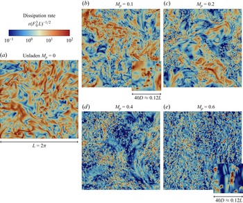
 ε(F03L)−1/2
 L2=(2π)2
 [10−1,102]
 Mp=0.1
 0.2
 0.4
 0.6
 40D≈0.12L
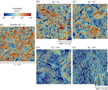
 ELF0−1
 L2=(2π)2
 [102,105]
 Mp=0.1
 0.2
 0.4
 0.6
 40D≈0.12L
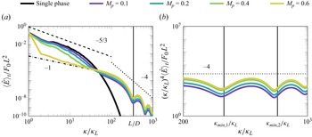
 a
 ⟨E^⟩t
 b
 (κ/κL)4⟨E^⟩t
 Mp
 κL=2π/L
 F0L2
 (κ/κL)−5/3
 (κ/κL)−1
 (κ/κL)−4
 a
 κD/κL=L/D
 b
 κmin,m=mπ/D
 m∈N

 ⟨⋅⟩t
 ⟨⋅⟩V,t
 Mp
 ⟨K⟩V,t
 ⟨ε⟩V,t
 ⟨η⟩t
 ⟨τη⟩t
 ⟨λ⟩t
 ⟨Reλ⟩t
 ⟨L⟩t
 ⟨τL⟩t
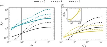
 Sn
 n=2
 n=4
 n=6
 Mp=0.2
 a
 Mp=0.6
 b
 D/η
 b
 S2
 log(r/η)
 Mp=0.6

 ⟨S⟩t
 a
 ⟨K⟩t
 b
 Mp
 D/η
 S=0
 a
 K=3
 b
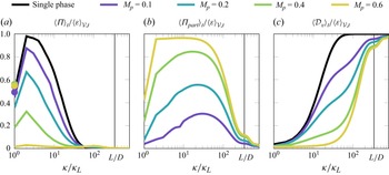
 ⟨Π⟩t
 ⟨Πpart⟩t
 ⟨Dv⟩t
 ⟨ε⟩V,t
 fiABC
 κ/κL=1
 ⟨P⟩t/⟨ε⟩V,t
 ◯
 κD/κL=L/D

 Φp=10−3
 Ψp=ρp/ρf
 Mp
 ΨpD2F01/2/(18νfL1/2)
 Rep≪1
 Stη=τp/⟨τη⟩t
 τp
 StL=τp/⟨τL⟩t
 StL0=τp/⟨τL0⟩t
 Rep
 (U~iU~i)1/2(F0L)−1/2
 ⟨⋅⟩p,t
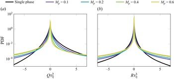
 a
 Q
 b
 R
 ∂jui
 Mp
 Q
 R
 τη
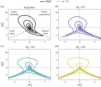
 Q
 R
 ∂jui
 Mp
 τη
 10−3
 101
 Q=−3(R/2)2/3
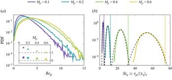
 Rep
 ◯
 △
 Rep
 Mp
 Stη≡τp/⟨τη⟩t
 Mp
 τp/⟨τη⟩t
 Stη
 Rep≪1
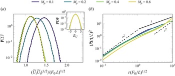
 a
 (U~iU~i)1/2
 (F0L)1/2
 ZU
 b
 [R(t)]2
 (L/F0)1/2
 L
 [R(t)]2∼t2
 [R(t)]2∼t
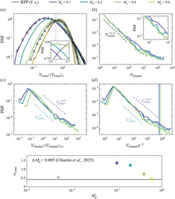
 a
 Vvoro/⟨Vvoro⟩V
 Ψp
 Mp
 △
 Ψp=5
 Mp=0.005
 ♢
 Ψp=100
 Mp=0.1
 b
 Ncluster
 50
 c
 ⟨Vcluster⟩V,t
 −2
 −16/9
 d
 η3
 −2
 −16/9
 ⟨L⟩t3⟨η⟩t−3
 σvoro
 Mp
 ◯
 Mp=0.005
 △

 σ
 S
 K
 Vvoro/⟨Vvoro⟩V
 ⟨Vcluster⟩V,t1/3⟨η⟩t−1
 ⟨Ncluster⟩V,t
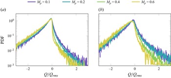
 Q/Qrms
 Mp
 Q
 a
 Dshell=3D
 b
 Dshell=6D
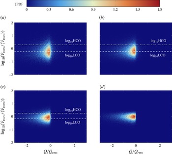
 Q
 Vvoro/⟨Vvoro⟩V
 a
 Mp=0.1
 b
 Mp=0.2
 c
 Mp=0.4
 d
 Mp=0.6
 Q
 Dshell=3D

 Open access

