INTRODUCTION
The impacts of climate change on insect communities in forestry and agriculture have been discussed frequently in the literature during the last few years (Netherer & Schopf Reference Netherer and Schopf2010; Thomson et al. Reference Thomson, Macfadyen and Hoffmann2010). These encompass impacts on species distribution (Ward & Masters Reference Ward and Masters2007), influences on arthropod–plant interaction (Yuan et al. Reference Yuan, Himanen, Holopainen, Chen and Stewart2009) or impacts on species life cycles (Musolin Reference Musolin2007; Kocmánková et al. Reference Kocmánková, Trnka, Eitzinger, Dubrovský, Štěpánek, Semerádová, Balek, Skalák, Farda, Juroch and Žalud2011). The potential impact of climatic change on the distribution of pest species in oilseed rape (Brassica napus L.) has been discussed recently by Olfert & Weiss (Reference Olfert and Weiss2006) for Canada. However, investigations on the influence of climatic change on pests in winter oilseed rape in Europe are still lacking.
The cabbage stem weevil, Ceutorhynchus pallidactylus (Mrsh.) (Coleoptera: Curculionidae), is one of the most severe pest species in winter oilseed rape (Alford et al. Reference Alford, Nilsson, Ulber and Alford2003). A detailed overview about its biology is given by Williams (Reference Williams and Williams2010). The species is univoltine (one generation per year) with three larval instars. Adults migrate from the overwintering habitats into crops of oilseed rape in early springtime. After a short time of feeding to permit ovary maturation, the female of C. pallidactylus oviposits egg batches into petioles and mid-ribs of leaves. The larvae mine within the pith of host plants; mature larvae migrate to soil for pupation at the end of May. The adult weevils emerge from soil at the end of June or beginning of July. After feeding on wild and cultivated brassicaceous plants for 4 weeks, they migrate to their overwintering sites (Williams Reference Williams, Horwitz and Ishaaya2004). C. pallidactylus passes through an obligate, pre-reproductive diapause before oviposition in the following spring. This species is widely distributed in Central Europe (Alford et al. Reference Alford, Nilsson, Ulber and Alford2003) and also common in Luxembourg (Braunert Reference Braunert2009).
So far, the migration from the overwintering habitat to crops of oilseed rape has been described by simple threshold-based models based on air and soil temperature (Günthart Reference Günthart1949; Nolte Reference Nolte and Hannemann1957) and precipitation (Broschewitz Reference Broschewitz1985) time series. Weather-based forecast models are commonly used as decision support tools for farmers in integrated pest management (Johnen et al. Reference Johnen, Williams, Nielsson, Klukowski, Luik, Ulber and Williams2010). However, these models may also be used to analyse the effects of projected changes in air temperature and precipitation for different time spans in the future.
The objective of the present study was to evaluate potential changes in the migration of the cabbage stem weevil into crops of oilseed rape under future regional climatic conditions in Luxembourg up to the year 2098, compared with the reference time span of 1961–1990. Several statistical threshold-based models for migration of C. pallidactylus were chosen from the literature and combined with regional climate model (RCM) simulation results from the EU ENSEMBLES project (http://ensemblesrt3.dmi.dk/, last accessed 18 March 2011, verified 19 April 2011) in order to analyse the impacts of changing air and soil temperatures and precipitation on this species.
MATERIALS AND METHODS
Biological models
All biological models used in the present study were chosen based on the availability of the meteorological input data (minimum, maximum and mean daily air temperature, daily totals of precipitation and daily mean soil temperature).
A threshold-based statistical relationship defined by Nolte (Reference Nolte and Hannemann1957) for describing the emerging of C. pallidactylus from overwintering sites and main migration to the crops of oilseed rape was used. This relationship is based on the mean daily soil temperature at a depth of 50 mm, which must reach at least 10·0°C to trigger the first activities of the weevil in its overwintering habitat. For the main migration, the daily maximum air temperature must exceed 15·0°C (Nolte Reference Nolte and Hannemann1957).
The model by Broschewitz (Reference Broschewitz1985) was used to describe the first catches of the cabbage stem weevil in yellow water traps. First observation of individuals of C. pallidactylus in crops of oilseed rape can be made on days with a daily mean temperature exceeding 12·0°C. A simple degree-day model was used to describe the development of plant phenology under climate change conditions (Alpmann Reference Alpmann2009). This threshold-based model was derived from long-term air temperature measurements from 35 different meteorological stations spread all over Germany. All daily air temperature values over a threshold value of 0.0°C were summed. In oilseed rape, 2641 degree-days are required from sowing to harvest, and a specific number of degree-days are necessary to complete a single phenological phase. According to Alpmann (Reference Alpmann2009), 287 degree-days are required to reach the stem elongation growth stage; this value was used in the present paper.
Biological observations
Field observations on the pest species migration results from a multi-location monitoring campaign, carried out in Luxembourg between 2007 and 2010, were used to compare with the modelled time points (in the reference period) of migration of C. pallidactylus. Individuals of C. pallidactylus were caught at five locations in Luxembourg (Burmerange (49°29′N, 6°19′E, 222 m asl), Obercorn (49°31′N, 5°51′E, 313 m asl), Useldange (49°46′N, 5°57′E, 307 m asl), Christnach (49°47′N, 06°16′E, 313 m asl) and Reuler (50°03′N, 06°02′E, 472 m asl)). At each location eight yellow water traps, set up along the field borders in areas where no insecticide was applied during the growing season, were used. All traps were checked and the insects caught collected twice per week.
The trap design was as follows: size 300×300×150 mm, height adjustable from ground level to 1·7 m above ground (upper edge) using a set of exchangeable aluminium rods. Three small drainage holes (3·0 mm in diameter) on each side panel ensured a constant water volume in the trap of about 3 litres even during rainfall. A small quantity of soap was added to the water, to break the surface tension and drown the insects. The captured individuals were stored in plastic containers in a 70% ethanol solution, and identified and counted using a binocular microscope.
Phenological data of oilseed rape at the five sample plots were recorded by measuring the growth stage (Lancashire et al. Reference Lancashire, Bleiholder, Van den Boom, Langelüddeke, Stauss, Weber and Witzenberger1991) during the biweekly field visits during the growing season.
Meteorological observations
Different meteorological observational datasets were used in the present study. Observations of daily mean air temperature were available from the airport station at Luxembourg-Findel (World Meteorological Organization station ID=06590). Daily values of mean air temperature and total precipitation from the International Commission for the Hydrology of the Rhine Basin dataset (named CHR-OBS; van der Linden & Mitchell Reference Van der Linden and Mitchell2009; Görgen et al. Reference Görgen, Beersma, Buiteveld, Brahmer, Carambia, de Keizer, de Krahe, Nilson, Lammersen, Perrin and Volken2010) were used for the bias correction of the RCM outputs (see below). Daily values of mean, minimum and maximum air temperature (2 m), mean soil temperature (50 mm depth) and total precipitation (1 m) were taken from stations of the operational meteorological network of the ‘Administration des Services Techniques de l'Agriculture’ (ASTA) at Reuler, Obercorn and Useldange.
RCM datasets
By using an ensemble of several regional climate change projections, it is possible to derive bandwidths of possible changes and thereby also assess the uncertainty associated with the projected changes. This is currently considered a good-practice approach in impact studies.
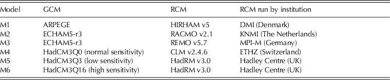
A selection of regional climate change projections from the Research Theme 2B of the EU-FP6 ENSEMBLES project (van der Linden & Mitchell Reference Van der Linden and Mitchell2009) was used (Table 1). In a dynamical downscaling, the RCM is driven by a global climate model (GCM), which is in turn influenced by a specific emission scenario.
Overview of six regional climate change projection simulation results used in the study. The model abbreviation used in the present paper is given, as well as the driving GCM and the RCM whose outputs are used. All GCMs are driven by the A1B emission scenario; RCM spatial resolution: 25×25 km, temporal resolution: daily means and totals; time-spans used for all RCMs: 1961–2098
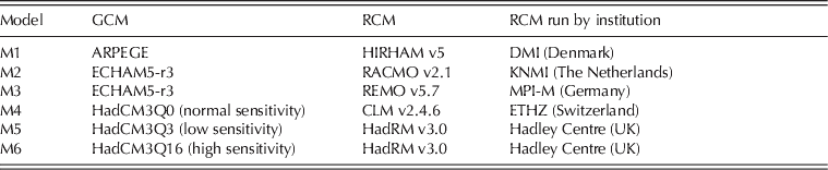
Two selection criteria for choosing a subset of the available RCM simulation results were used. First, only RCM outputs with a 25×25 km spatial resolution, based on a model chain with an A1B emission scenario were used. The IPCC A1B emission scenario (IPCC Reference Solomon, Qin, Manning, Chen, Marquis, Averyt, Tignor and Miller2007) describes anthropogenic emissions of a future world with rapid economic growth, an increasing global population until the mid of this century and a balanced use of fossil and non-fossil energy resources. It is widely used in impact assessments due to data availability.
Secondly, a relatively large proportion of the overall ensemble bandwidth in terms of precipitation and air temperature change signals must be covered by the RCMs in the presently considered ensemble in order to account for many different possible future climate evolutions. This is partly achieved by the large variety of GCM–RCM combinations.
This way, some of the most widely used European RCMs are represented in the present study. The temporal coverage of the datasets used here extends from 1961 to 2100. The time span up to 2000 is considered as the ‘control time span’ (based on observed 20th century emission data) followed by the ‘projected time span’ (based on the A1B emission scenario). As the HadCM3-driven RCM temporal coverage ends in November and December 2099, respectively, the far future time span is defined from 2069 to 2098, and the near future time span is defined from 2021 to 2050. Variables retrieved are daily mean air temperature, daily minimum and maximum air temperature as well as daily total precipitation.
RCM data processing
To derive spatial means, all grid cells on the differing model output grids (all with 25 km grid resolution) that overlap with the area of Luxembourg were averaged, using a weighting factor per grid element, based on the respective overlap area.
RCM outputs are, for many reasons, biased in comparison with observational datasets. Therefore, it was necessary to bias-correct them before using them with an impact model (Piani et al. Reference Piani, Haerter and Coppola2010), especially as threshold-driven processes were to be investigated, which require absolute values instead of relative changes. A non-linear bias correction approach was used to correct daily precipitation; air temperature was corrected with a linear-scaling approach. Both approaches are described in detail in Nilson et al. (Reference Nilson, Beersma, Perrin, Carambia, Krahe, de Keizer, Görgen, Görgen, Beersma, Brahmer, Buiteveld, Carambia, de Keizer, Krahe, Nilson, Lammersen, Perrin and Volken2010a). The respective correction factors were determined for the reference time span (1961–90); the bias correction was applied afterwards to the complete time series (1961–2100). The validity and suitability of the bias correction methods applied in the present paper are shown by Nilson et al. (Reference Nilson, Perrin, Beersma, Krahe, Carambia, de Keizer, Görgen, Görgen, Beersma, Brahmer, Buiteveld, Carambia, de Keizer, Krahe, Nilson, Lammersen, Perrin and Volken2010b).
Because the available CHR-OBS reference dataset does not include daily minimum and maximum air temperatures, which would allow for a distinct bias correction of these RCM variables, a linear regression model was used to derive relationships among uncorrected RCM daily mean air temperatures and uncorrected daily minimum and maximum air temperature. This relationship was then applied to the corrected RCM daily mean air temperature in order to derive those missing variables.
Soil temperature data
For some threshold-based biological models, soil temperature at a depth of 50 mm depth is required. As this variable was not available as RCM model output, a non-linear statistical relationship between measured soil temperature, air temperature and precipitation at three automatic stations (ASTAs) at Obercorn, Reuler and Useldange was used to derive this information.
Artificial neural networks (ANNs) have been applied successfully in various environmental studies (Bryant & Shreeve Reference Bryant and Shreeve2002; Junk et al. Reference Junk, Feister and Helbig2007; Ramirez-Beltran et al. Reference Ramirez-Beltran, Castro, Harmsen and Vasquez2008). ANNs imitate the human brain's problem-solving ability by applying knowledge gained from past experience and previously solved examples to new problems by building a system of ‘neurons’ that takes new decisions and provides predictions. It normally consists of three layers (input layer, hidden layer and output layer), which are fully interconnected by communication links associated with weights that determine the effect on the information passing through them.
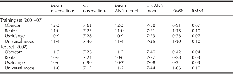
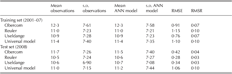
Here, eight predictors in the input layer (day of year, daily precipitation, mean, minimum and maximum values of air temperature as well as the air temperature values – including minimum and maximum – from the day before), one hidden layer and one target or output variable were used. In the first step, independent ANN models for each of the three ASTAs used were set up to make sure that results were comparable (Table 2).
Soil temperature statistics for each individual neural network for the three ASTA stations as well as for the combined universal model, including the root mean square error (RMSE) and its proportional value (RMSR). Training dataset ranges from 2001 to 2007 (N=7421) and the independent test dataset is of 2008 (N=1086)
s.d.: Standard deviation.
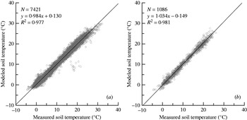
After that, the time series of the three ASTAs were combined to derive a universal statistical relationship between the predictors and the soil temperature for Luxembourg. The dataset (daily values) for the model set up covers the period 2001–07 (N=7421) and was divided into three subsets, a training set (15% of the data), a production set (70% of the data) and a test set (15% of the data). Furthermore, the year 2008 (N=1086) was used as a totally independent dataset for the model validation. Figs 1(a) and 1(b) show scatter plots between modelled and measured soil temperature data for 50 mm depth. While Fig. 1(a) shows the results for the training period 2001–07, Fig. 1(b) presents results for the independent test year 2008. Surprisingly, the results for the independent test year 2008 are slightly better than those for 2001–07. This might be attributed to a lower frequency of extreme values within the observations of that year. In general, the universal model shows satisfactory results (Table 2).
Scatter plots of measured and modelled soil temperatures, derived from three meteorological stations, equally spread over Luxembourg. (a) training dataset=daily data from 2001 to 2007, (b) validation dataset=daily data for 2008.

In the second step, the universal ANN model was hence used to derive the required soil temperature time series from the bias corrected RCM model outputs.
RESULTS
Projected air temperature changes in Luxembourg
The Grand Duchy of Luxembourg covers an area of 2586 km2 and is located in Western Europe, surrounded by France, Belgium and Germany. The country is characterized by a temperate semi-oceanic climate with mild winters and moderate summers. Increases in maximum and minimum air temperatures for the second half of the 20th century for Luxembourg have already been forecasted (Drogue et al. Reference Drogue, Mestre, Hoffmann, Iffly and Pfister2005), and similarly Pfister et al. (Reference Pfister, Drogue, El Idrissi, Iffly, Poirier and Hoffmann2004) suggested increasing winter rainfall amounts caused by a higher frequency of westerly circulation types for the same time span.
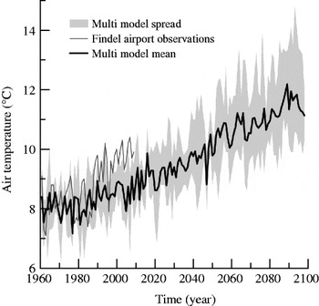
Figure 2 illustrates the spatially averaged annual mean air temperatures for Luxembourg for the selected ENSEMBLES RCMs. The multi-model ensemble bandwidth is expressed by the absolute minimum and maximum of the six-member distribution (grey shading). To summarize the ensemble's evolution, the multi-model arithmetic mean is shown (black line). The observations from the Findel airport station are also shown (dark grey line) as a rough indication that the model results agree with observations. Due to the small ensemble size (N=6 RCMs), no statistical measures of the distribution were derived.
Temporal evolution of annual mean air temperature: multi model (N=6) bandwidth (grey shading); multi-model mean (black line) with long-term annual mean from 1961 to 1990=8·1°C and Findel airport observatory (dark grey) with long-term annual mean from 1961 to 1990=8·3°C.

The measured annual mean air temperatures at the airport station (long-term mean from 1961 to 1990=8·3°C) correspond very well with the model results (long-term mean from 1961 to 1990=8·1°C). From 2000 onwards the measured values are on the upper end of the multi-model spread, suggesting that the air temperature projections at the beginning of the 21st century are already a conservative estimate of observed changes during the last decade.
Cabbage stem weevil
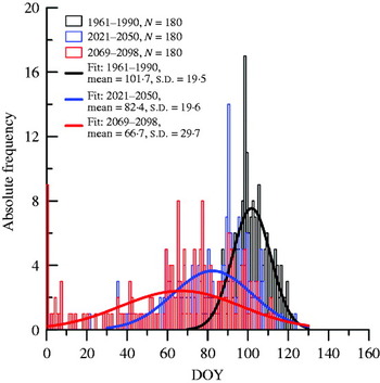
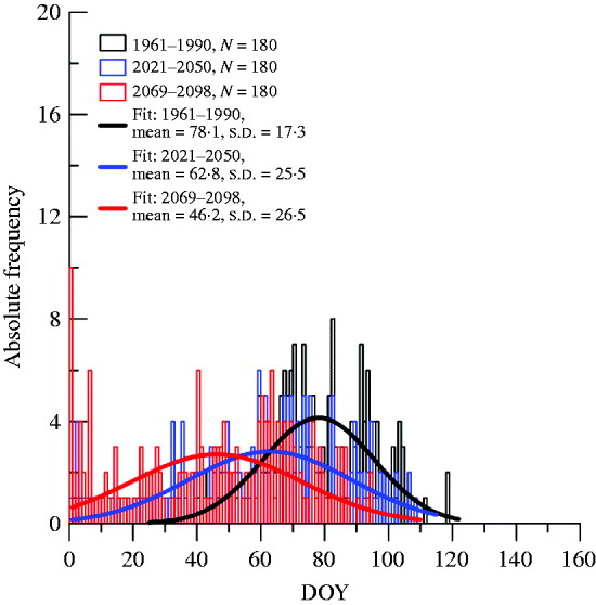
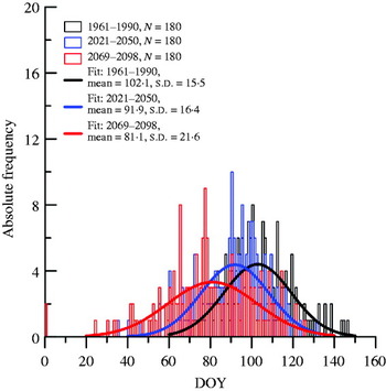
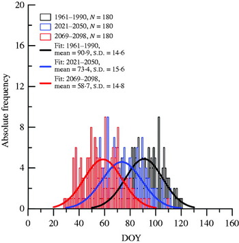
The following results are presented as absolute frequency distributions for three different time spans: the reference period (1961–90), the near future time span (2021–50) and the far future (2069–98). Each frequency distribution consists of the annual event – expressed as day of the year (DOY) – for each year and model, leading to 180 elements per frequency distribution (30 years for each of the six models). Since nine of the 12 frequency distributions shown in Figs 3–6 are normally distributed, empirical Gaussian distribution functions are fitted for an easier interpretation of the change signals.
Using the threshold-based model of Nolte (Reference Nolte and Hannemann1957), clear differences between the three time spans for the emergence of C. pallidactylus (Fig. 3) can be suggested. In the control time span, emergence was on average at DOY 102 (12 April). For the two future time spans, shifts towards earlier dates were derived: DOY 82 (23 March) for the near future and DOY 67 (8 March) for the far future (Fig. 3).
Absolute frequency of the DOY when C. pallidactylus emerges from the overwintering habitat and shows first activity (Nolte Reference Nolte and Hannemann1957; threshold: mean daily soil temperature of 10°C at a depth of 50 mm), derived from 30-year time spans and six RCMs (N=180, all available annual data combined into a single distribution). Fitted to the absolute frequency distributions are empirical Gaussian distribution functions for the three time spans from 1961 to 1990 (black line), 2021 to 2050 (blue line), and 2069 to 2098 (red line). Means and s.d. of the distribution functions are also given in the corresponding colours.

Also, the duration of the projected time span for the emergence of C. pallidactylus may be prolonged from 60 days in the past (reference period) to 100 days (near future) and 130 days (far future), respectively.
Using the threshold-based model of Broschewitz (Reference Broschewitz1985), a similar temporal displacement from DOY 78 (19 March, reference period) to DOY 63 (4 March, near future) and to DOY 46 (15 February, far future) was suggested (Fig. 4). Simple comparisons of the results for the reference time span indicate DOY 78±17·3 (means±s.d.) days. This agrees well with in situ observations for the years 2007–2010 (DOY 76±15·2).
Absolute frequency of the DOY for the first observation of C. pallidactylus in crops of oilseed rape (Broschewitz Reference Broschewitz1985; threshold: mean daily air temperature >12°C), derived from 30-year time spans and six RCMs (N=180, all available annual data combined into a single distribution). Fitted to the absolute frequency distributions are empirical Gaussian distribution functions for the three time-spans from 1961 to 1990 (black line), 2021 to 2050 (blue line) and 2069 to 2098 (red line). Means and s.d. of the distribution functions are also given in the corresponding colours.
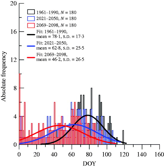
The projected period in which the first individuals of cabbage stem weevil could be observed in the field was prolonged from 90 days up to 140 days in the near future time span. For the far future projections, first occurrence of the pest species can be expected at the beginning of the year (Fig. 4).
To determine the point in time for the main migration of C. pallidactylus to oilseed rape fields, another threshold-based model of Nolte (Reference Nolte and Hannemann1957) was used. The main migration during the reference period (1961–99) was around DOY 102 (12 April, Fig. 5). For the two future time spans, shifts towards earlier dates in the near (DOY 92, 2 April) and far future (DOY 81, 22 March) were found. Again a comparison with in situ observations revealed slightly less agreement than above, with DOY 90±16·7 for the field observations from 2007 to 2010 and DOY 102±15·5 for the model results during the reference time span.
Absolute frequency of the DOY for the main migration of C. pallidactylus in crops of oilseed rape (Nolte Reference Nolte and Hannemann1957; threshold: mean daily air temperature >15°C), derived from 30-year time spans and six RCMs (N=180, all available annual data combined into a single distribution). Fitted to the absolute frequency distributions are empirical Gaussian distribution functions for the three time spans from 1961 to 1990 (black line), 2021 to 2050 (blue line) and 2069 to 2098 (red line). Means and s.d. of the distribution functions are also given in the corresponding colours.

The period for the main migration of C. pallidactylus is extended only for the far future projections (30 days): the near future projection only showed a slight shift towards an earlier onset, albeit no significant extension (Fig. 5).
Plant development
According to Alpmann's plant development model (Alpmann Reference Alpmann2009), a temporal displacement from DOY 91 (1 April, reference period) to DOY 73 (14 March, near future) and to DOY 59 (28 February, far future) can be found for the stem elongation growth stage (Fig. 6). These results were also compared with field observations, showing good agreements with DOY 90±13·0, for the period 2007–10 and model results of DOY 91±14·6 for the reference period.
Absolute frequency of the DOY for the growth stage stem elongation rate of oilseed rape (B. napus) according to Alpmann (Reference Alpmann2009), derived from 30-year time spans and six RCMs (N=180, all available annual data combined into a single distribution). Fitted to the absolute frequency distributions are empirical Gaussian distribution functions for the three time spans from 1961 to 1990 (black line), 2021 to 2050 (blue line) and 2069 to 2098 (red line). Means and s.d. of the distribution functions are also given in the corresponding colours.

Based on the projected air temperatures for the future time spans, the duration of this growth stage is not likely to be prolonged, only shifted towards an earlier onset (Fig. 6).
DISCUSSION AND CONCLUSION
Climate change impacts on anthropogenic and natural systems have been observed at all spatial scales. Climate projections based on different emission scenarios and simulated with GCMs and RCMs indicate that these impacts are likely to increase. The ENSEMBLES project indicates, e.g. rising air temperatures close to the earth's surface and decreasing amounts of precipitation during the summer months for Central and Northern Europe (van der Linden & Mitchell Reference Van der Linden and Mitchell2009). These changes will have impacts on economically cultivated plants and on pest insects in the near and far future (Reid Reference Reid2006; Estrella et al. Reference Estrella, Sparks and Menzel2007; Parmesan Reference Parmesan2007; Eitzinger et al. Reference Eitzinger, Orlandini, Stefanski and Naylor2010).
The present study investigates the possible effects of regional climate change on the migration of the cabbage stem weevil into crops of oilseed rape, based on ensembles of regional climate change projections for Luxembourg.
Pest species and diseases can reduce crop productivity in agriculture (Oerke Reference Oerke2006), and strategies for minimizing yield losses under climate change conditions are in great demand (Berry & Spink Reference Berry and Spink2006; Barnes et al. Reference Barnes, Wreford, Butterworth, Semenov, Moran, Evans and Fitt2010). Several studies on plant herbivores under climate change conditions deal with future species distributions within a country (Estay et al. Reference Estay, Lima and Labra2009; Roura-Pascual et al. Reference Roura-Pascual, Brotons, Peterson and Thuiller2009). Regional projections on species activity in crops of host plants are still rare, because of a lack of ensembles of RCM projections with the necessary spatial resolutions. Thanks to efforts like the ENSEMBLES project (van der Linden & Mitchell Reference Van der Linden and Mitchell2009), such data are increasingly becoming available.
The study focused on the plant–pest interaction in early springtime: emergence of C. pallidactylus from overwintering habitats and migration to crops of oilseed rape. The cabbage stem weevil has an obligate diapause in winter (Williams Reference Williams and Williams2010). A diapause in an insect's development is a genetically programmed response to environmental conditions (Bale & Hayward Reference Bale and Hayward2010). It ends for most species in mid-winter, followed by a kind of quiescence (Hodek Reference Hodek1996), before environmental conditions are favourable for the insect. Increasing air temperature can shorten the diapause (Bale & Hayward Reference Bale and Hayward2010) and may lead to earlier emergence and activity in overwintering habitats.
Based on the projected increasing air temperature, a shift of nearly 32 days towards earlier emergence from the 30-year reference period to the far future time span can be expected, corresponding to a shift of about 3·3 days per decade. It has been predicted that when the increase in mean air temperature reaches 3°C, the diapause of the cabbage stem weevil, Ceutorhynchus obstrictus (Marsham) in Canada will shift forward by 2 weeks (Olfert & Weiss Reference Olfert and Weiss2006).
For the first migration of C. pallidactylus to crops of oilseed rape, an advance of 3 days per decade was derived. This effect was quite similar to the results for the first activity in overwintering habitats. An earlier emergence during spring under climate change conditions has been described for other insect species (van Asch et al. Reference Van Asch, van Tienderen, Holleman and Visser2007; Bale & Hayward Reference Bale and Hayward2010). However, it is not clear which parameter has most influence. A species-specific combination of day length, temperature combined with insufficient stored nutrient resources is likely (Hodek Reference Hodek1996). The photoperiod seems to be less important for C. pallidactylus, because its overwintering habitat under leaf and litter in the wood is described as ‘shady’, which dampens air temperature fluctuations and amplitudes (Skrocki Reference Skrocki1972).
For the main migration period of C. pallidactylus to crops of oilseed rape, an advance of nearly 21 days was found from the reference period to the far future. A shift of the main migration period of pest species in agriculture under projected climate change conditions has been predicted for invertebrate species in general (Root et al. Reference Root, Price, Hall, Schneider, Rosenzweig and Pounds2003), and in detail for the cabbage root fly, Delia radicum (Collier et al. Reference Collier, Finch, Phelps and Thompson1991) and for some butterfly species on brassicaceous host plants (Roy & Sparks Reference Roy and Sparks2000). However, the shift of the main migration period for C. pallidactylus corresponds with an earlier phase of emergence in overwintering habitats and the first migration to the crops.
Period of migration
Threshold-based statistical relationships between meteorological variables and insect development states were established based on the results by yellow water traps as a tool to aid timing of pesticide application (Williams Reference Williams and Williams2010). An appropriate date for insecticide application before the phase of oviposition is a main prerequisite for successful chemical control of the cabbage stem weevil (Seidenglanz et al. Reference Seidenglanz, Poslušná and Hrudová2009). A single insecticide application before flowering is usually enough to control the cabbage stem weevil (Williams Reference Williams and Williams2010). In comparison with other pests, e.g. the pollen beetle (Meligethes aeneus Fabricius), the main migration of the cabbage stem weevil culminates in a short time-span only (Lehmann Reference Lehmann1965), which makes a single pesticide application possible. As an additional effect, the adults of another ceutorhynchid stem weevil, the rape stem weevil (Ceutorhynchus napi Gyll.), are also targeted by the same application (Fröhlich Reference Fröhlich1956; Lehmann Reference Lehmann1965). However, the present results revealed that the phase of the migration of C. pallidactylus to crops of oilseed rape in early springtime may be prolonged in the future. With an extended period of migration, the risk of missing the appropriate time for an insecticide application is therefore higher.
As a future research objective in this context, the migration phase of C. napi under climate change conditions will also be analysed in order to check whether the co-presence of both ceutorhynchid stem weevils could still happen in the future.
Plant phenology and crop–pest synchrony
Plant phenology depends primarily on air temperature (Chmielewski et al. Reference Chmielewski, Müller and Bruns2004). Agricultural crops seem to be affected less by climate effects in comparison with perennial plants (Estrella et al. Reference Estrella, Sparks and Menzel2007). A significant shift of nearly 4 days per 1°C air temperature in the beginning of the flowering and harvest periods of oilseed rape under climate change conditions may be expected (Estrella et al. Reference Estrella, Sparks and Menzel2007). The projections indicate a shift of 3·0 days per decade with respect to the phenological phase of the stem elongation.
The synchrony of host plant and herbivore can be important for the pest status of a species (van Asch et al. Reference Van Asch, van Tienderen, Holleman and Visser2007). In the present study, a continued synchrony of pest species and host plant even for the far future is suggested, because a shifting of about 3 days per decade is predicted for both. However, C. pallidactylus is not strongly dependent on a highly specific development stage of the host plant, because of its oviposition behaviour in leaf petioles (Williams Reference Williams and Williams2010). In contrast, for C. napi, a close interaction between oviposition and the host plant architecture was found (Büchi Reference Büchi1996). C. napi prefers the main stems of oilseed rape up to 220 mm in height for oviposition. Higher plants were not infested and lateral racemes were not chosen. Regional climate changes might influence this synchrony between host plant and herbivore. However, examples for possible restoration of synchrony by genetic adaptation have already been shown for the winter moth, Operophthera brumata L. (van Asch et al. Reference Van Asch, van Tienderen, Holleman and Visser2007).
Biological models
Since the 1950s, several phenological models have been developed to describe the migration of C. pallidactylus into crops of oilseed rape in springtime (Johnen et al. Reference Johnen, Williams, Nielsson, Klukowski, Luik, Ulber and Williams2010). Different parameters have been reported to influence its activity, e.g. temperature and precipitation (Nolte Reference Nolte and Hannemann1957), wind speed (Kjaer Reference Kjaer, Menken, Visser and Harrewijn1992) and sunshine hours (Nolte Reference Nolte and Hannemann1957). Different models of species phenology use wind speed and sunshine duration as additional input variables (Johnen et al. Reference Johnen, Williams, Nielsson, Klukowski, Luik, Ulber and Williams2010). Unfortunately, these models could not be integrated into the present study because the required input data were not available.
For the present study, projections of future precipitation, and air and soil temperature were available. Pest phenological models in decision support systems mostly deal with ‘if then’ rules and indices for identifying favourable conditions for possible migrations to field crops (Johnen et al. Reference Johnen, Williams, Nielsson, Klukowski, Luik, Ulber and Williams2010). Hence, the state of the art in this regard does not represent an accurate numerical model of pest phenology dependent on climatic conditions. However, most of these models are based on different studies from different European regions from the past 60 years and have been adapted to local conditions. Contradictions between different pest models have already been discussed by Debouzie & Wimmer (Reference Debouzie and Wimmer1992).
A comparison of the model output with the present results by field trapping showed slightly different time points for the main migration of C. pallidactylus. A calibration of the biological models to the regional climate conditions in Luxembourg could eliminate these uncertainties, but longer time series of field observations are necessary.
A simple and reliable model for describing the different growth stages of winter oilseed rape is lacking. The model by Alpmann (Reference Alpmann2009) is limited to temperature and based on accumulated degree-days. Nevertheless, this model was chosen because the required input variables were available and comparisons between model results and field observations agreed well. However, the photoperiod can accelerate the phase of elongation as an additional variable (Andrew et al. Reference Andrew, Tommey and Evans1991).
Ensemble projections
The simulation results of GCMs need to be regionalized with adequate downscaling methodologies, e.g. RCMs, to have regional climate change projections available that make a derivation of potential impacts on ecological systems possible (Marletto et al. Reference Marletto, Ventura, Fontana and Tomei2007). The present study used the selected model outputs from the ENSEMBLES project. The advantages and disadvantages of using ensemble projections for describing impacts of potential climate change on shifts in species communities and distributions have been shown in the literature (Araújo & New Reference Araújo and New2007; Buisson et al. Reference Buisson, Thuiller, Casajus, Lek and Grenouillet2010). As the RCM outputs are biased, adequate bias corrections are needed before they are used to drive impact models. A detailed overview of the different bias correction methods used in the present study is given by Nilson et al. (Reference Nilson, Perrin, Beersma, Krahe, Carambia, de Keizer, Görgen, Görgen, Beersma, Brahmer, Buiteveld, Carambia, de Keizer, Krahe, Nilson, Lammersen, Perrin and Volken2010b).
An increase in high performance computing power makes larger and more spatially resolved climate change ensembles possible. Instead of relying on the results of only a single model chain realization, an ensemble of model runs, either different model combinations (e.g. different GCM and RCM combinations as used in the present study) or the same GCM with slightly different initial conditions and/or physical settings can be used for climate projections.
At the expense of extended computing times associated with higher costs, the ensemble approach permits a better estimation of the uncertainties associated with the climate projections. Also, using ensembles of future climate projections leads to more accurate estimates of the potential future changes since the effect of the internal variability can be more accurately addressed (May Reference May2008). However, despite these projections, the real range of possible future changes is still unknown.
We are grateful to the ‘Administration des Services Techniques de l'Agriculture’ (ASTA) for financial support. The study was partly funded by the FNR CORE 2009 CLIMPACT project (FNR C09/SR/16). We are grateful to Ludger Alpmann (DSV-Deutsche Saatveredelung) for providing data concerning plant phenology. Special thanks to Jules Beersma from the Royal Netherlands Meteorological Institute (KNMI), De Bilt, The Netherlands for providing datasets within the CHR/RheinBlick2050 project. We thank the two anonymous reviewers for their comments, which helped to improve the manuscript.